Estimation of Soil Moisture Index Using Multi-Temporal Sentinel-1 Images over Poyang Lake Ungauged Zone


1
State Key Laboratory of Information Engineering in Surveying, Mapping and Remote Sensing, Wuhan University, Wuhan 430079, China
2
School of Remote Sensing and Information Engineering, Wuhan University, Wuhan 430079, China
3
Jiangxi Provincial Meteorological Observatory, Jiangxi Meteorological Bureau, Nanchang 330046, China
4
The Key Laboratory of Poyang Lake Wetland and Watershed Research, Ministry of Education, Jiangxi Normal University, Nanchang 330022, China
*
Author to whom correspondence should be addressed.
Remote Sens. 2018, 10(1), 12; https://doi.org/10.3390/rs10010012
Submission received: 15 November 2017
/
Revised: 6 December 2017
/
Accepted: 20 December 2017
/
Published: 22 December 2017
(This article belongs to the Special Issue Retrieval, Validation and Application of Satellite Soil Moisture Data)
Abstract
:The C-band radar instruments onboard the two-satellite GMES Sentinel-1 constellation provide global measurements with short revisit time (about six days) and medium spatial resolution (5 × 20 m), which are appropriate for watershed scale hydrological applications. This paper aims to explore the potential of Sentinel-1 for estimating surface soil moisture using a multi-temporal approach. To this end, a linear mixed effects (LME) model was developed over Poyang Lake ungauged zone, using time series Sentinel 1A and 1B images and soil moisture ground measurements from 15 automatic observation sites. The model assumed a linear relationship that varied with both time and space between soil moisture and backscattering coefficient (SM-). Results showed that three LME models developed with different polarized images all meet the European Space Agency (ESA) accuracy requirement for GMES soil moisture product (≤5% in volume), with the vertical transmit and vertical receive (VV) polarized model achieving the best performance. However, the SM- relationship was found to depend strongly on space, making it difficult to predict absolute soil moisture for each grid. Therefore, a relative soil moisture index was then proposed to correct for site effect. When compared with those of the linear fixed effects model, the soil moisture indices predicted by the LME model captured the temporal dynamics of measured soil moisture better, with the overall R2 and cross-validated R2 being 0.68 and 0.64, respectively. These results indicate that the LME model can be effectively applied to estimate soil moisture from multi-temporal Sentinel-1 images, which is useful for monitoring flood and drought disasters, and for improving stream flow prediction over ungauged zones.
1. Introduction
As an “Essential Climate Variable”, as identified by the Global Climate Observing System, soil moisture plays a critical role in the water and energy balance at the soil-atmosphere boundary, which has a large effect on climate [1,2]. At a watershed scale, soil moisture also controls the partitioning of rainfall into runoff and infiltration, and therefore has an important effect on the runoff response of catchments [3]. Hence, soil moisture has been widely used in various applications, such as numerical weather forecasting [4], water and energy budgets simulation [5], soil evaporation evaluation [6], stream flow prediction [7], and water resource management [8]. Located in the south bank of the middle reaches of the Yangtze River, Poyang Lake is the largest freshwater lake of china. The ungauged zone of Poyang Lake, which lacks hydrological observations, generally refers to the large alluvial plain stretching from seven stream flow gauging stations to the lake boundary. This region covers a majority of the Poyang Lake eco-economic zone, which is occupied by intensive rice agriculture, supporting the high-density local population. Moreover, the significant seasonal fluctuations of Poyang Lake water levels and the associated inundation areas create extensive wetland ecosystems in this region [9]. However, both droughts and floods have occurred frequently around the lake in recent decades, which are primarily caused by climate change and human activities [10]. For example, the severe continuous drought during 2006–2007 brought the lake water storage down to less than 1% of the lake capacity [11], and the extrema flood event in 1998 resulted in direct economic losses of about ¥38 billion over the Poyang Lake watershed [12], with most of the losses occurring within the ungauged zone. Accordingly, soil moisture estimation over Poyang Lake ungauged zone is of vital importance for flood forecasting and drought monitoring, irrigation scheduling, agriculture management, and wetland protection. Besides, knowledge of soil moisture is beneficial to the Predictions in Ungauged Basins (PUB) researches [13].
Soil moisture, especially surface soil moisture, is highly variable in space and time [14]. In situ measurements can provide accurate estimation of soil moisture, but they are both time consuming and expensive, and only represent a small area (few square decimeters). Nevertheless, a number of strategies can be adopted to upscale the spatially sparse ground-based observations [15,16], which are invaluable for calibrating and validating land surface models and satellite-based soil moisture retrievals [17]. Microwave remote sensing techniques have been used to obtain surface soil moisture, commonly referred to as the water content of the uppermost soil layer, at various temporal and spatial scales since the 1970s [18]. The strengths lie in that both microwave scattering and emission are directly related to the water content of soil surface and microwave sensors can acquire imagery in all weather, during day and night. In recent years, various soil moisture products have been derived globally from microwave radiometer and scatterometer systems with high temporal resolution [19,20,21,22], but they are generally too coarse for watershed or field scale applications. Using downscaling techniques, the spatial resolution of those soil moisture products can be largely improved, while uncertainties can be introduced during this process [23,24]. Conversely, Synthetic Aperture Radar (SAR) systems can achieve much higher spatial resolutions (<1 km) and allow for soil moisture mapping at fine scales directly. However, apart from soil moisture, SAR measurements are also sensitive to several other surface parameters such as surface roughness, vegetation cover, and topography, making it difficult to separate the soil moisture contribution to the backscatter signal from other factors. Therefore, based on different SAR configurations and available surface parameters, various empirical, semi-empirical, and theoretical models have been proposed to retrieve soil moisture at regional scales over the last few decades [25,26,27]. Developed by ESA to ensure continuity of C-band SAR data, the Sentinel-1 constellation features a temporal resolution of six days and spatial resolution of 5 × 20 m over land [28], which are appropriate for soil moisture estimation over Poyang Lake ungauged zone. Currently, several algorithms have been proposed to retrieve soil moisture operationally from Sentinel-1 data, using change detection techniques [29,30], Bayesian approach [31], and Artificial Neural Network (ANN) [32], respectively. Both change detection and Bayesian methods exploit the short revisit time of Sentinel-1 data and assume that the backscatter cross section of soil surfaces changes over short timescales, mainly due to variations in soil moisture, while the average characteristics of surface roughness remain almost unaltered [31]. This assumption might be invalidated by the pronounced heterogeneity of soil surfaces when estimating soil moisture from Sentinel-1 data at full spatial resolution. The ANN algorithm trained with theoretical model can retrieve soil moisture accurately from single SAR acquisition, but a robust and extensive reference dataset for the training of the ANN technique is essential, which is lacking for most areas [32].
In this paper, a linear mixed effects model is developed to estimate surface soil moisture from multi-temporal Sentinel-1 images. It is assumed in the first place that a linear relationship exists between surface soil moisture and the backscattering coefficient in logarithmic units for bare and vegetated surfaces. This linear relationship might be affected by several time and space varying parameters, such as terrain, vegetation, and soil properties. It is assumed then that variability in the SM- relationship can be accounted for by introducing the LME model, which has been successfully applied in the prediction of particulate matter with aerodynamic diameter ≤2.5 μm (PM2.5) using satellite aerosol optical depth (AOD) products [33,34,35,36]. Under these assumptions, time series Sentinel-1 backscatter images and ground soil moisture measurements over Poyang Lake ungauged zone are used to calibrate the LME model, in which the SM- relationship varies both by time and space. The paper is organized as follows. In Section 2, the study area and the datasets of radar and ground measurements are briefly introduced. Section 3 describes both the linear mixed and fixed effects models, and then proposes a soil moisture index. Performance comparisons between different models and validation of the model predicted soil moisture indices are shown in Section 4. Section 5 discusses the results, and Section 6 draws the main conclusions.
2. Study Area and Datasets
2.1. Study Area
As the largest freshwater lake in China, Poyang Lake is also one of the most important wetlands in the world, which has been recognized by the International Union for Conservation of Nature [37]. Five main tributaries (Ganjiang, Fuhe, Xiushui, Xinjiang, and Raohe) flow into Poyang Lake and then discharge into the Yangtze River from south to north, owing to a higher elevation in the south. Poyang Lake ungauged zone consists of the ungauged watersheds between seven stream flow gauging stations (Qiujin, Wanjiabu, Waizhou, Lijiadu, Meigang, Hushan and Dufengkeng) of the five tributaries and the boundary of Poyang Lake, as illustrated in Figure 1a. The detailed method of drawing the watersheds in the ungauged zone is presented in [38]. SAR images have been repeatedly collected over Poyang Lake by Sentinel-1 sensors, and the overlapping area of these images acquired at different times is chosen as the study area (Figure 1b), which covers a majority of the ungauged zone. The region is characterized by a subtropical monsoon climate with wet season from April to September, and dry season from October to March [39]. The annual average temperature is 17.5 °C, and the annual average accumulative precipitation is approximately 1680 mm [40]. Due to the seasonality of precipitation and other meteorological conditions, Poyang Lake’s inundation area varies significantly from >3100 km2 during the wet season to <750 km2 during the dry season [39,41]. While the peripheral areas are mountainous, covered largely by dense forests, the alluvial plains surrounding the lake are mainly used as cultivated cropland. Floods and droughts have occurred frequently around the Poyang Lake in recent years, posing a great threat to natural and economical resources, or even to human lives. Watershed scale soil moisture product with high temporal resolution is essential for the predicting and monitoring of these disasters.
2.2. Sentinel-1 Data
Sentinel-1 is a two-satellite constellation carrying C-band (λ = 5.6 cm) SAR instruments to ensure data continuity that began with the ERS and Envisat satellites [42]. Sentinel-1A was launched on 3 April 2014, operating in a near-polar, sun-synchronous orbit with a 12-day repeat cycle and 175 orbits per cycle. Then, Sentinel-1B, sharing the same orbit plane with a 180° orbital phasing difference, was launched on 25 April 2016. Currently, with both satellites operating, an ideally six days revisit time can be achieved in most of the regions [43]. Sentinel-1 has four exclusive acquisition modes: Strip Map (SM), Interferometric Wide swath (IW), Extra Wide swath (EW), and Wave (WV) modes. Over land, the Sentinel-1 SAR instruments, with the exception of emergency situations, operate in IW mode by default, which provides a wide coverage of 250 km with a spatial resolution of 5 × 20 m in range and azimuth directions, respectively [43].
The Sentinel-1 mission provides open-access data to users with a very low latency. All data can be freely downloaded through the Copernicus Open Access Hub [44]. A total of 49 Sentinel-1A/1B SAR images were selected over the study area from April 2015 to December 2016. These images were acquired in IW mode at both VV and VH (vertical transmit and horizontal receive) polarizations. Moreover, all of the images are in ascending pass (track 40), with incidence angle ranging from 30.8° to 45.9°. Level-1 Ground Range Detected (GRD) product, which consists of focused SAR data that has been detected, multi-looked (5 × 1 looks), and projected to ground range using an Earth ellipsoid model, is used in this study. The spatial resolution of high-resolution GRD product is about 20 × 22 m, and the corresponding pixel spacing is 10 × 10 m in range and azimuth directions, respectively [43]. Although Sentinel-1 SAR sensors are assumed to acquire images day and night regardless of weather conditions, it is sometimes hard for C-band signals to penetrate through thick clouds or severe storms. Therefore, two images acquired on 17 June 2015 and 12 February 2016 were removed, both of which were partially affected by the bad weather. Table 1 lists the acquisition dates, the gaps between consecutive images (∆days) and the sensor types (A or B) of the Sentinel-1 images used.
Preprocessing of the Sentinel-1A/1B images were performed with the open source SNAP software (version 4.0) [45], as provided by ESA, which included a collection of Sentinel-1 specific processing tools. The workflow was divided into several steps. First, precise orbit files were downloaded and were applied to the raw images to obtain accurate satellite position and velocity information. Then, the adjacent slices of the same days were put together using the S-1 Slice Assembly tool. Second, radiometric calibration was performed to convert digital pixel values into backscattering coefficients. Third, to reduce the inherent speckle noise of SAR images, both multi-looking processing (2 × 2 looks) and speckle filtering (Refined Lee filter) [46] were conducted. Fourth, Range-Doppler terrain correction was done with the Shuttle Radar Topography Mission (SRTM) 3 arc-seconds data [47] to correct for geometric distortions, producing orthorectified images with 20 × 20 m resolution in Universal Transverse Mercator (UTM) projection (Zone 50 N). Fifth, the time series images were co-registered to a master image (18 April 2015) in the Stack tool, outputting the minimum extent of all images. Then, these backscattering images were converted from linear scale to logarithmic scale (dB).
2.3. Ground Measurements
Over the study area, there are 17 automatic soil moisture observation sites that are equipped with the DZN1 sensors [48], installed and maintained by Jiangxi meteorological bureau. The DZN1 sensors are based on the Frequency Domain Reflectometry (FDR) technique, which derives soil moisture content on the basis of changes in the frequency of signals due to the dielectric properties of the soil [49]. All of the sites are located in the local dominant cropland, including paddy field, dryland, nursery, and orchard. At each site, volumetric soil moisture measurements are taken up to a depth of 80 cm, every 10 cm, with an hourly time interval. Among the 17 sites, two of them were screened out in suspicion of data exception. The remaining sites were also checked carefully for implausible measurements and outliers, discarding three records at last. To match the passing time and penetration depth of Sentinel-1 satellites, soil moisture records of the 15 sites measured in 10:00 a.m. at the depth of 0–10 cm were used. The spatial distribution of the mean surface soil moisture of these sites is shown in Figure 1b, and the descriptive statistics of each site is provided in Table 2. In addition, daily temperature and precipitation measurements collected at site 9 (Nanchang) were obtained from the China Meteorological Data Sharing Service System [50].
3. Methods
3.1. Linear Mixed Effects Model
For bare soil surfaces with given soil condition (roughness or texture), radar backscattering is found to be linearly dependent upon the volumetric soil moisture in the upper few centimeters [51]. Over vegetated surfaces, the return signal depends both on the volume scattering of vegetation and on the attenuated backscattering from the underlying soil. As in [52], we assumed a linear SM- relationship for both bare and vegetated soil surfaces
where, is the backscattering coefficient of bare or vegetated surfaces in logarithmic scale and is the surface soil moisture. The parameter A is the sensitivity of the backscattering coefficient to changes in soil moisture content, which is primarily related to the vegetation cover and varies seasonally with the vegetation cycle. The parameter B is a function of soil roughness and vegetation cover effects on radar signal, which varies strongly in both space and time. Unlike some other empirical models that considered the regression parameters as constant, we added random effects to the parameters, allowing for them to vary temporally and spatially. This could be realized by introducing the linear mixed effects model with random slopes and intercepts.
The underlying premise of linear mixed effects models is that some subset of the regression parameters varies randomly from one individual to another, thereby accounting for sources of natural heterogeneity in the population. The distinctive feature of linear mixed effects models is that the mean response is modelled as a combination of population characteristics that are assumed to be shared by all the individuals, and subject-specific effects that are unique to a particular individual [53]. The former are referred to as fixed effects, while the latter are referred to as random effects. To represent the varying SM- relationship, a LME model was developed using the soil moisture ground measurements and the collocated Sentinel-1 backscattering coefficients. The LME model regressed as a predictor of SM by including day-specific random intercepts and slopes for , and site-specific random intercepts for spatial adjustment. The basic form of the model can be expressed as follows:
where is the soil moisture at a spatial site i on a day j, is the backscattering coefficient of the grid cell corresponding to site i on the same day; and are the fixed and random day-specific intercepts, respectively; and are the fixed and random day-specific slopes, respectively; is the random intercept of site i; is the error term at site i on a day j, and, is the variance-covariance matrix for the day-specific random effects. Making use of the restricted maximum likelihood method, the fixed and random parameters in the LME model were estimated using the “lmer” function in the lme4 package for R [54].
The effect of polarization on the SM- relationship was inspected by comparing the LME models developed using different polarized images, which were VV polarization, VH polarization and VV + VH polarizations, respectively. Moreover, the LME models with and without the site-specific term were compared to provide a measure of the sensitivity of the model-derived time varying SM- relationship to site locations.
Another approach that allows for the SM- relationship to vary temporally would be fitting a linear fixed effects model separately for each day when both radar image and soil moisture measurements are available. The linear fixed effects model follows the form of
where and are the fixed intercept and slope on a day j, respectively; is the error term on a day j. In this model, the SM- relationship is constant for all of the sites on a certain day and the spatial differences are not considered. Model performances of the linear mixed and fixed effects models were compared to reveal whether the LME model was able to improve the prediction of soil moisture.
3.2. Soil Moisture Index
Time series soil moisture maps are supposed to be predicted by applying the LME model, developed above with the calibrated fixed and random parameters, to each grid cell over the study area. However, it is usually difficult to get the site-specific random intercepts for each grid, due to the strong spatial variability of soil moisture. Therefore, a relative soil moisture index was proposed to correct for site effect and normalized volumetric soil moisture to a dimensionless index between 0 and 1. The soil moisture index was calculated using the following equation:
where is the soil moisture index on a day j for a certain grid, is the measured or predicted volume soil moisture on a day j for the same grid, , and are the maximum and minimum values of the grid in the measured or predicted soil moisture time series, respectively. Soil moisture indices predicted by both the linear mixed and fixed effects models were validated by those calculated with ground measurements to investigate the temporal agreements.
3.3. Model Validation
Both the LME models and the linear fixed effects model were validated against ground measurements using the following statistics: R2, root-mean-square error (RMSE), mean prediction error (MPE), temporal R2, and spatial R2 [35]. MPE was estimated as the mean absolute differences between predicted and measured soil moisture. Temporal R2 was calculated by regressing Delta SM against Delta predicted where: Delta SM is the difference between measured soil moisture at site i on day j and the mean measured soil moisture at site i, and Delta predicted is defined similarly for the predicted values generated from the models. Spatial R2 was calculated by regressing the mean measured soil moisture at site i against the mean predicted soil moisture at site i. Furthermore, a cross-validation method was adopted to test the stabilities of the linear mixed and the fixed effects models in predicting the soil moisture index. Specifically, the data of one site (test site) were separated from those of the other 14 sites (calibration sites). The models were trained with the data from the calibration sites and then predicted soil moisture indices for the test site. This process was repeated until each of the 15 sites was tested, and cross-validated R2 values between predicted and measured soil moisture indices were then calculated.
4. Results
4.1. Model Fitting and Comparison
A total of 727 soil moisture and backscattering coefficient data pairs from 15 observation sites on 49 imaging days are available for model fitting. Based on the Equation (2), three LME models were developed using of different polarization combinations: VV polarization, VH polarization, and VV + VH polarizations. Table 3 shows the calibrated parameters and performance statistics of these LME models. For the VV polarized model, the fixed effects of the intercept and slope () are statistically significant with = 33.36 (p < 0.001) and = 0.33 (p < 0.001), respectively. The standard deviations of the day-specific intercepts and slopes are 2.04 and 0.13, respectively, with that of the site-specific intercepts being 6.83. For the VH polarized model, while the fixed term of the intercept is still significant with = 32.54 (p < 0.001), the fixed effect of the slope () is nonsignificant with = 0.13 (p = 0.175). The VV polarized model gains a slightly higher R2 and smaller RMSE and MPE when compared with the VH polarized model. Combining both VV and VH polarizations in the LME model, the performance of the VV + VH polarized model is slightly worse than the single polarized models, obtaining the lowest R2 and the largest RMSE and MPE. In the VV + VH polarized model, while the fixed effects of the intercept and the VV polarized slope () are statistically significant, with = 32.98 (p < 0.001) and = 0.34 (p < 0.001), respectively, the fixed effect of the VH polarized slope () is nonsignificant with = −0.03 (p = 0.749). This is probably because VH polarization is more sensitive to volume scattering from vegetation canopies and multiple surface scattering from rough surfaces [55]. Although all of the three LME models meet the ESA accuracy requirement of 5% [32] for GMES soil moisture product, VV polarization achieves the best performance, and is hence used in the following LME models.
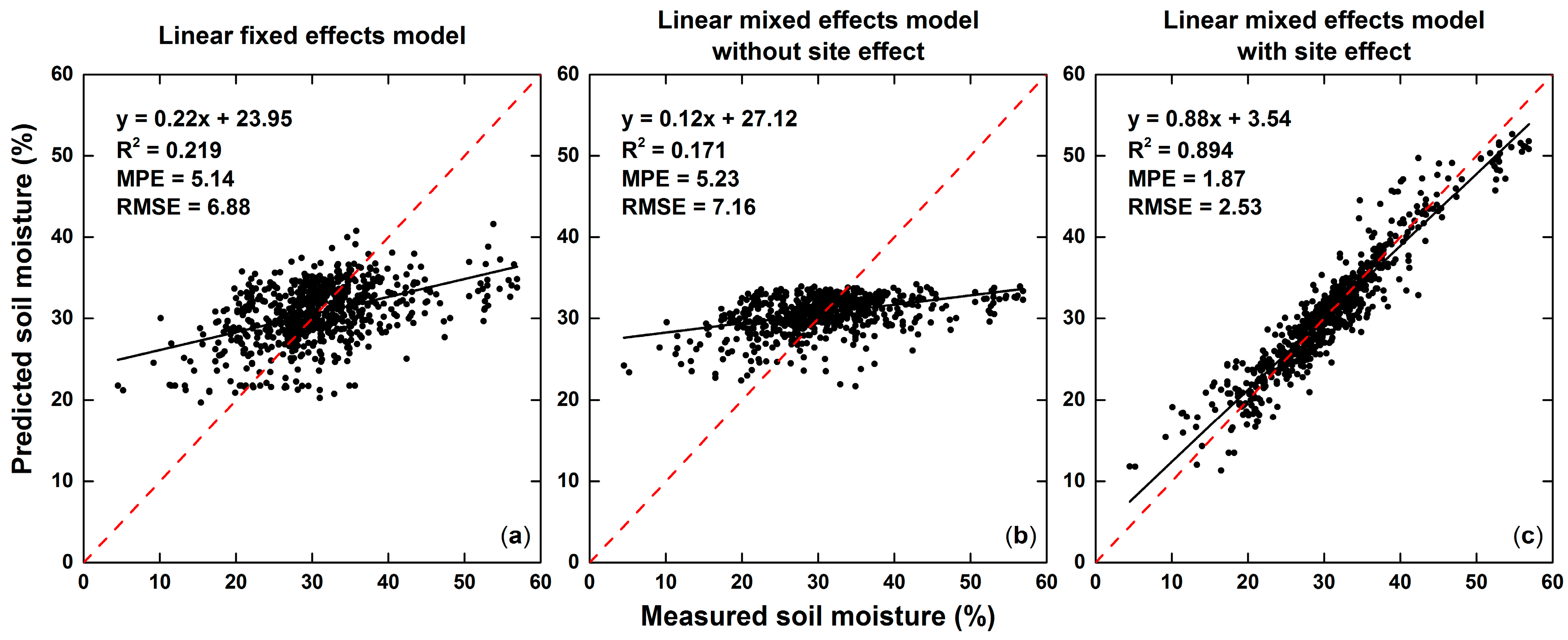
Based on the Equation (3), a linear fixed effects model was developed using the same set of soil moisture and backscattering coefficient data pairs. The performance statistics of this model are shown in the Table 4. Without considering the spatial differences in the SM- relationship, although the linear fixed effects model obtains a satisfying temporal and spatial R2, the MPE achieved is very large. This results in the relatively low overall R2 and large RMSE, and the latter fails to meet the 5% accuracy requirement. Nevertheless, with a temporal R2 of 0.56, the fixed effects model is supposed to capture the temporal variations of soil moisture to some extent. In contrast, the full LME model achieves both higher temporal and spatial R2 and lower MPE, significantly improving the overall R2 and RMSE to 0.89 and 2.53%, respectively. To further study the sensitivity of the SM- relationship to site locations, the site-specific term was removed from the full LME model. As shown in Table 4, the spatial R2 of the LME model without the site-specific term drops dramatically to 0.052, leading to the lowest overall R2 and largest RMSE and MPE of the three models. The large differences between measured soil moisture and those that were predicted by the linear fixed effects model and the mixed effects model without site effect can also be seen from Figure 2. When compared with the other two models, the mixed effects model with site effect (Figure 2c) significantly increases the slope of the linear regression between predicted and measured soil moisture, making the regression line much closer to the 1:1 line. It indicates that accounting for site effect in the LME model is necessary to improve the predicted soil moisture accuracy, due to the strong spatial variability of surface soil moisture. When compared with the linear fixed effects model, the temporal R2 of the LME model without the site-specific term rises from 0.56 to 0.61, owing to a more stable daily SM- relationship calibrated using data pairs from all days. The full LME model further improves the temporal R2 to 0.64, which is expected to better characterize the temporal variations of soil moisture and chosen to derive the soil moisture index in the following sections.
4.2. Soil Moisture Index Estimation and Validation
Soil moisture indices were calculated for each of the 15 observation sites, based on the Equation (4), using soil moisture time series measured and predicted from the linear mixed and fixed effects models, respectively. As an example, the temporal variation of soil moisture index derived from ground measurements, along with the daily accumulated precipitation and mean temperature over site 9 (Nanchang) are plotted in Figure 3. The daily mean temperature shows a similar pattern for the year 2015 and 2016, with the highest temperature observed between July and August and the lowest temperature between January and February. The precipitation increased significantly between April and June in both years. Moreover, due to the El Niño event, precipitation occurred frequently from the winter of 2015 to the spring of 2016. Calculated with soil moisture measurements at the depth of 0–10 cm, which represents the uppermost soil layer, the measured soil moisture indices are rather sensitive to precipitation and temperature. In response to the El Niño event and the lower evaporation rate during the non-growing season, the measured soil moisture indices over site 9 remained high from December 2015 to June 2016. In contrast, with the higher evaporation rate during the growing season and little precipitation, the measured soil moisture indices decreased dramatically from July to August in both years.
Figure 4 shows the measured soil moisture index curve of each site (black solid lines). All of the curves vary remarkably with time, reflecting the strong temporal variability of surface soil moisture during the study period. On the other hand, the soil moisture index curves of different sites share a similar pattern, which is supposed to be related to the large scale atmospheric factors, such as precipitation and evapotranspiration. During the period from April 2015 to December 2016, the measured soil moisture index curves generally start with several irregular fluctuations and rise rapidly in November 2015, followed by a plateau till June 2016, and then drop sharply to the bottom in August or September 2016 and rise again gradually till the end of 2016. Unlike regular years with little precipitation during dry season from October to March, the winters of both years were rainy over the whole study area, leading to the relatively high soil moisture indices. In addition, the decreasing soil moisture indices in August of both years could be attributed to the constantly high temperature and low precipitation.
The soil moisture index curves that were predicted by the linear fixed effects model (blue dash lines) and the LME model (red dash lines) are also presented in Figure 4. For each site, both of the predicted curves capture the major trends of the measured soil moisture index curve well, with that of the LME model fitting the measured curve better. The R2 value of the LME model at each site ranges from 0.52 to 0.88, totally exceeding that of the fixed effects model, which ranges from 0.44 to 0.81. At most sites, the LME model largely improves the R2 by reducing the bias between the measured and predicted soil moisture indices. However, both of the models achieve relatively low R2 values at site 4 (Xingzi) and site 5 (Fengcheng), since the two sites are located near buildings or ponds, and might be less representative than other sites.
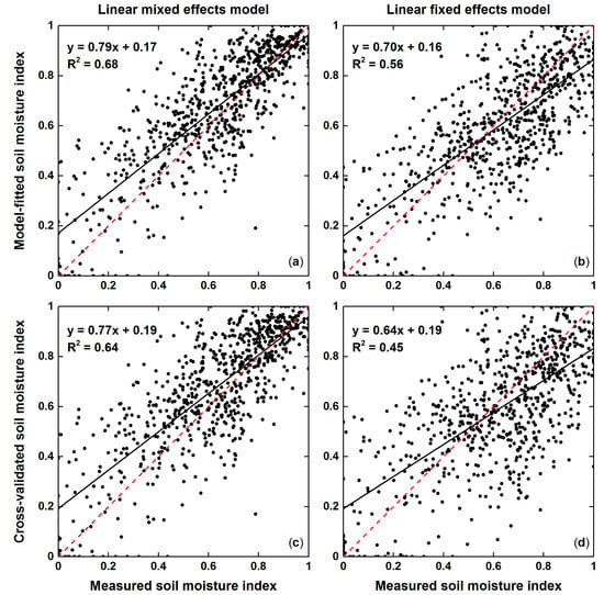
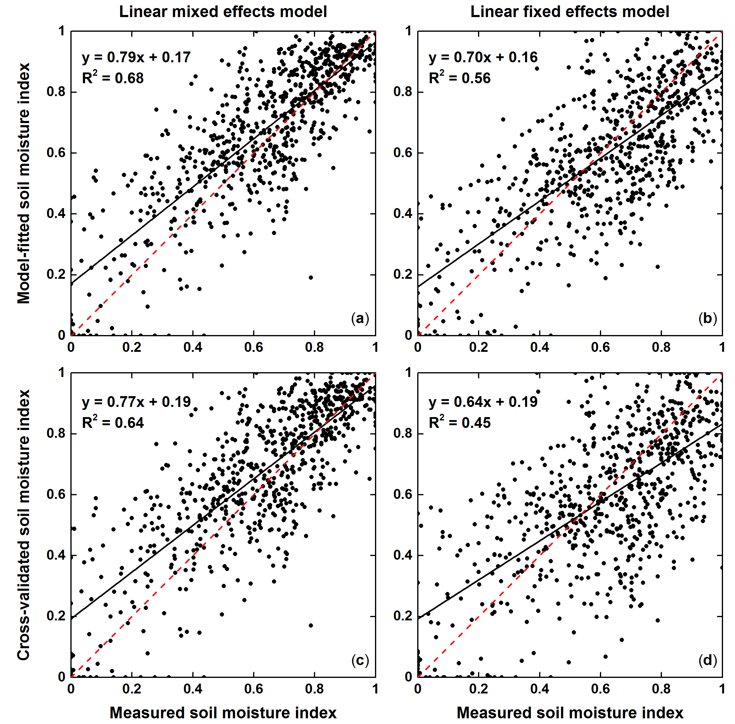
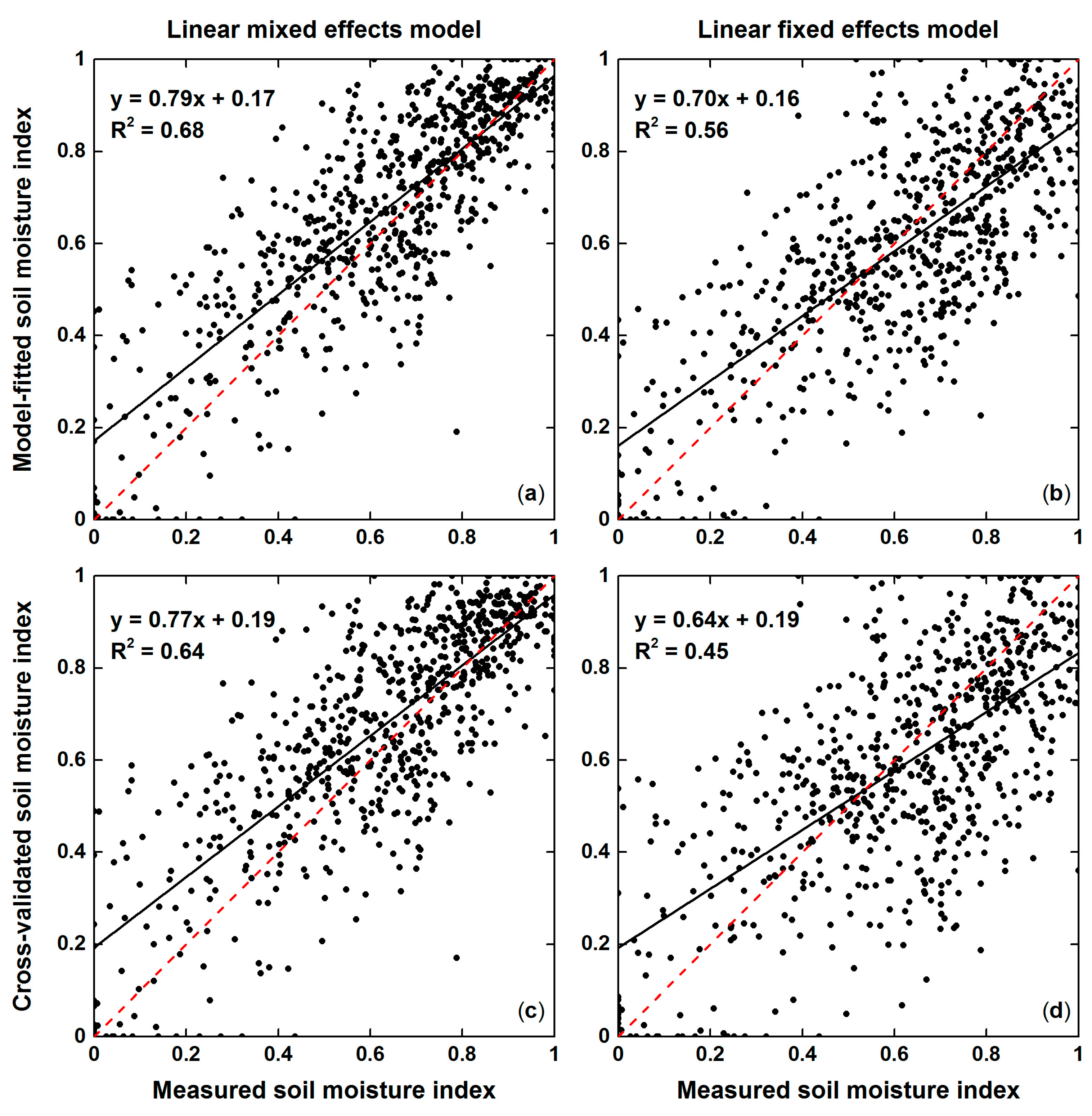
Figure 5 shows the overall accuracies of soil moisture indices predicted by the linear mixed and fixed effects models. The overall R2 and cross-validated R2 of the linear fixed effects model are 0.56 (Figure 5b) and 0.45 (Figure 5d), respectively. In contrast, both the values increase considerably in the LME model, which are 0.68 (Figure 5a) and 0.64 (Figure 5c), respectively. Both models have a larger prediction error for the lower soil moisture index, which might be partly due to the shallower observation depth of C-band microwaves than ground measurements. Since the upper layer of soil is more subjected to rapid drying and rewetting, soil moisture variations in this layer are more pronounced [56], especially under the drier conditions. When compared with that of the fixed effects model, the cross-validated R2 of the LME model is only slightly lower than its overall R2, indicating a more robust performance of the LME model. Moreover, the LME model increases the slopes of the linear regressions between the predicted and measured soil moisture indices, making the regression lines closer to the 1:1 lines when compared with those of the fixed effects model, which further demonstrates the better prediction ability of the LME model.
4.3. Soil Moisture Index Maps
After calibrated the full LME model using 727 soil moisture and backscattering coefficient data pairs, the day-specific intercepts and slopes could be estimated, which were applied to the time series backscattering images to derive soil moisture maps over the study area. It should be noted that, since the site-specific term was not available for each grid, it was removed from the calibrated LME model when predicting soil moisture maps. Based on the Equation (4), a total of 49 soil moisture index maps were finally produced from the predicted soil moisture maps. With meaningless soil moisture index values, the water bodies and urban areas on each map were extracted and masked individually, making use of their distinctive backscattering characteristics. The spatial mean and coefficient of variation (CV) of soil moisture index were then calculated for each map, respectively. Basically, the CV tends to increase with decreasing mean soil moisture index (Figure 6), which suggests the higher spatial variability of soil moisture index under the drier conditions. The trend of the CV can be fitted by a decreasing power function, with a high coefficient of determination (R2 = 0.988). Similar decreasing trend has been found for the CV of absolute soil moisture by many studies that were carried out in humid climates, which is related to the parameters of the moisture retention characteristic and their spatial variability. [1,57,58]. As there are large areas of irrigated paddy fields around the Poyang Lake, the more pronounced spatial differences of soil moisture between irrigated and non-irrigated fields might also contribute to the higher CV under the drier conditions. Figure 6 also shows the distinctive seasonal differences of the CV. In winter and spring, the mean soil moisture index is higher and less variable, whereas in summer and autumn, both the mean and CV of soil moisture index are highly variable.
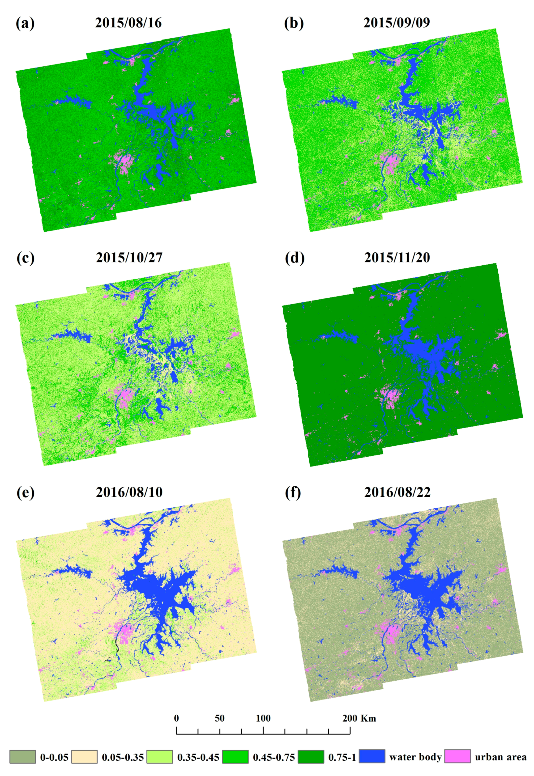
Among the 49 soil moisture index maps, six were selected to show the spatial distribution of soil moisture index under different soil moisture conditions (Figure 7). Since very few rain events occurred during late August to early September in 2015, the mean soil moisture index decreased from 0.75 on August 16 (Figure 7a) to 0.45 on September 9 (Figure 7b). More significant spatial variability can be observed from the soil moisture index map on September 9 (Figure 7b), where the soil moisture indices of the alluvial plains surrounding the Poyang Lake, which are mainly used as cultivated cropland, are much lower than those of the peripheral areas that covered largely by forests. It might be attributed to the different water-holding capacities of cropland and forest. Due to the frequent rainfall during November 2015, both the inundation area and the soil moisture index increased significantly on November 20 (Figure 7d), compared with those on October 27 (Figure 7c). Almost no spatial difference can be found in the soil moisture index map on November 20 (Figure 7d), when the moisture content over the whole region was nearly saturated. The mean soil moisture index decreased sharply from 0.33 on August 10 (Figure 7e), to almost zero on August 22 (Figure 7f), which is supposed to be related to the constantly high temperature and low precipitation during August 2016. Most of the areas suffered from drought during this period of time, while the croplands around the water bodies achieve slightly higher values on both soil moisture index maps, probably because of irrigation.
5. Discussion
Based on the LME model, we explored the potential for soil moisture retrieval over Poyang Lake ungauged zone using time series Sentinel-1 images. Although several algorithms have been proposed to retrieve soil moisture maps operationally from Sentinel-1 data recently, our method is different in that it assumes a linear SM- relationship varied with both time and space. The accuracies of three LME models developed using different polarized images (Table 3) all meet the ESA requirement for GMES soil moisture product (≤5%). Moreover, after validating the model predicted soil moisture indices against those calculated with ground measurements, the performance statistics achieved are comparable with those from the existing similar studies [59,60], with the overall R2 and cross-validated R2 being 0.68 and 0.64, respectively.
The LME model has been widely used to account for daily variations of the AOD-PM2.5 relationship and shows good performance in model predictions. Since parameters that influence the AOD-PM2.5 relationship exhibit much less spatial variability than temporal variability, the LME model without the site effect shows similar performance when compared with the full LME model [34]. In contrast, the SM- relationship varies strongly in space and accounting for the site effect in the LME model is necessary to improve the predicted soil moisture accuracy, as shown in Table 4. However, when predicting soil moisture maps over the whole study area, the site-specific intercept was not available for each grid. Therefore, a relative soil moisture index was proposed to correct for site effect. The derived soil moisture indices of each site capture the temporal dynamics of the measured soil moisture indices well (Figure 4), which are usually of greater interest than their absolute values in some applications [61].
It is necessary to investigate the prediction uncertainties that are associated with this work. Possible sources of error are as follows: (1) soil moisture ground measurements. With a limited number of observation sites under which the main land cover class is cropland, it is difficult to fully characterize the soil moisture patterns over the study area. Besides, measurement errors of the DZN1 sensors also contribute to the uncertainties; (2) Different spatial scales between in situ points and satellite pixels. While soil moisture measurements that are used to calibrate the SM- relationship are collected at point scale, the collocated backscattering coefficients represent the average condition of the whole grid cell; (3) Different observation depths between the DZN1 sensor and C-band radar. Ground measurements that are used in this study are taken at the depth of 0–10 cm, whereas the penetration depth of C-band microwaves is about 0.5–2 cm [62]. This difference could bring uncertainties during the calibration and validation phases; (4) The LME model. Under the assumptions of a linear SM- relationship and as the single predictor, the developed LME model introduces uncertainties. Multiple factors affect the spatial variability and the temporal dynamic of soil moisture and most of these factors are interrelated, making it difficult to model all of the predictors.
Despite the uncertainties, the LME model that is developed in this study shows a better and more robust performance when compared with the linear fixed effects model (Figure 5). By allowing the SM- relationship to change temporally and spatially, the LME model accounts for other factors to some extent, such as vegetation and surface roughness. More predictors, such as NDVI and soil texture, can be added to the LME model to further study the spatial variation of the SM- relationship. Due to its simplicity, the model can be easily transferred to other regions with multi-temporal SAR images and soil moisture measurements. With more observation sites and longer time series Sentinel-1 images, the performance of the LME model is expected to be further improved.
6. Conclusions
The objective of this study was to generate surface soil moisture products from multi-temporal Sentinel-1 images. To this end, a linear mixed effects model was developed to establish the relationship between soil moisture ground measurements and Sentinel-1 backscattering coefficients over Poyang Lake ungauged zone. The major results of this work are summarized as follows.
(1) Three linear mixed effects models were developed using backscattering coefficients of VV polarization, VH polarization, and VV + VH polarizations, respectively. All of the three models meet the ESA accuracy requirement (≤5%), while the VV polarized model achieves the best performance, with an overall R2 of 0.89 and RMSE of 2.53%.
(2) The full linear mixed effects model was compared with the model without the site-specific term. Results show that site effect plays an important role in the soil moisture and backscattering coefficient relationship. Nevertheless, both of the models characterize the temporal variations of soil moisture rather well, and a slightly higher temporal R2 of 0.64 is obtained by the full linear mixed effects model.
(3) A relative soil moisture index was proposed to correct for site effect. Both the fixed and mixed effects models were applied to predict the soil moisture indices, which were then validated by the measured soil moisture indices. The R2 value of the mixed effects model at each observation site ranges from 0.52 to 0.88, totally exceeding that of the fixed effects model, which ranges from 0.44 to 0.81. Moreover, with the overall R2 and cross-validated R2 being 0.68 and 0.64, respectively, the linear mixed effects model shows a better and more robust performance in predicting the temporal dynamics of soil moisture, when compared with the fixed effects model.
Time series soil moisture product with appropriate spatial resolution is invaluable for watershed scale hydrological applications, especially over ungauged basins. The linear mixed effects model that is developed in this work shows the potential for estimating soil moisture from time series Sentinel-1 data in a simple and robust way. The model can be easily transferred to other watersheds, since the Sentinel-1 constellation provides C-band radar data globally, while soil moisture ground measurements are also needed for the calibration and validation of the model. Model prediction uncertainties mainly come from the limited ground observations and the assumptions of a linear soil moisture and backscattering coefficient relationship and backscattering coefficient as the single predictor. Further studies can be investigating the impact of more explanatory factors, such as vegetation and soil parameters, to have a better understanding of site effect.
Acknowledgments
This study was supported by grants from National Natural Science Funding of China (NSFC, 41331174), Major Science and Technology Program for Water Pollution Control and Treatment (2013ZX07105-005), and Surveying & Mapping and Geo-information Research in the Public Interest (No. 201512026). The authors would like to thank Copernicus Open Access Hub for providing Sentinel-1 data and China Meteorological Data Sharing Service System for the meteorological data used in the research. We are grateful for the instructive comments and suggestions provided by the two anonymous reviewers.
Author Contributions
Yufang Zhang, Xiaoling Chen and Jianya Gong conceived and designed the experiments; Yufang Zhang performed the experiments and analyzed the data; Kun Sun contributed the data analysis; Jianmin Yin helped to process the data; Yufang Zhang wrote the paper.
Conflicts of Interest
The authors declare no conflict of interest.
References
- Pratola, C.; Barrett, B.; Gruber, A.; Kiely, G.; Dwyer, E. Evaluation of a global soil moisture product from finer spatial resolution SAR data and ground measurements at Irish sites. Remote Sens. 2014, 6, 8190–8219. [Google Scholar] [CrossRef]
- Seneviratne, S.I.; Corti, T.; Davin, E.L.; Hirschi, M.; Jaeger, E.B.; Lehner, I.; Orlowsky, B.; Teuling, A.J. Investigating soil moisture-climate interactions in a changing climate: A review. Earth Sci. Rev. 2010, 99, 125–161. [Google Scholar] [CrossRef]
- Wagner, W.; Blöschl, G.; Pampaloni, P.; Calvet, J.-C.; Bizzarri, B.; Wigneron, J.-P.; Kerr, Y. Operational readiness of microwave remote sensing of soil moisture for hydrologic applications. Hydrol. Res. 2007, 38, 1–20. [Google Scholar] [CrossRef]
- Scipal, K.; Drusch, M.; Wagner, W. Assimilation of a ERS scatterometer derived soil moisture index in the ECMWF numerical weather prediction system. Adv. Water Resour. 2008, 31, 1101–1112. [Google Scholar] [CrossRef]
- Saux-Picart, S.; Ottlé, C.; Decharme, B.; André, C.; Zribi, M.; Perrier, A.; Coudert, B.; Boulain, N.; Cappelaere, B.; Descroix, L. Water and energy budgets simulation over the AMMA-Niger super-site spatially constrained with remote sensing data. J. Hydrol. 2009, 375, 287–295. [Google Scholar] [CrossRef]
- Zribi, M.; Chahbi, A.; Shabou, M.; Lili-Chabaane, Z.; Duchemin, B.; Baghdadi, N.; Amri, R.; Chehbouni, A. Soil surface moisture estimation over a semi-arid region using ENVISAT ASAR radar data for soil evaporation evaluation. Hydrol. Earth Syst. Sci. 2011, 15, 345–358. [Google Scholar] [CrossRef] [Green Version]
- Brocca, L.; Melone, F.; Moramarco, T.; Wagner, W.; Naeimi, V.; Bartalis, Z.; Hasenauer, S. Improving runoff prediction through the assimilation of the ASCAT soil moisture product. Hydrol. Earth Syst. Sci. 2010, 14, 1881–1893. [Google Scholar] [CrossRef]
- Komma, J.; Blöschl, G.; Reszler, C. Soil moisture updating by Ensemble Kalman Filtering in real-time flood forecasting. J. Hydrol. 2008, 357, 228–242. [Google Scholar] [CrossRef]
- Zhang, Q.; Ye, X.-C.; Werner, A.D.; Li, Y.-L.; Yao, J.; Li, X.-H.; Xu, C.-Y. An investigation of enhanced recessions in Poyang Lake: Comparison of Yangtze River and local catchment impacts. J. Hydrol. 2014, 517, 425–434. [Google Scholar] [CrossRef]
- Ye, X.; Zhang, Q.; Liu, J.; Li, X.; Xu, C.-Y. Distinguishing the relative impacts of climate change and human activities on variation of streamflow in the Poyang Lake catchment, China. J. Hydrol. 2013, 494, 83–95. [Google Scholar] [CrossRef]
- Ye, X.; Zhang, Q.; Bai, L.; Hu, Q. A modeling study of catchment discharge to Poyang Lake under future climate in China. Quat. Int. 2011, 244, 221–229. [Google Scholar] [CrossRef]
- Chen, Y.; Xiong, W.; Wang, G. Soil and water conservation and its sustainable development of the Poyang Lake catchment in view of the 1998 flood of Yangtze River. J. Sediment Res. 2002, 4, 48–51. [Google Scholar]
- Sivapalan, M.; Takeuchi, K.; Franks, S.; Gupta, V.; Karambiri, H.; Lakshmi, V.; Liang, X.; McDonnell, J.; Mendiondo, E.; O’connell, P. IAHS Decade on Predictions in Ungauged Basins (PUB), 2003-2012: Shaping an exciting future for the hydrological sciences. Hydrol. Sci. J. 2003, 48, 857–880. [Google Scholar] [CrossRef]
- Korres, W.; Reichenau, T.; Schneider, K. Patterns and scaling properties of surface soil moisture in an agricultural landscape: An ecohydrological modeling study. J. Hydrol. 2013, 498, 89–102. [Google Scholar] [CrossRef]
- Crow, W.T.; Berg, A.A.; Cosh, M.H.; Loew, A.; Mohanty, B.P.; Panciera, R.; Rosnay, P.; Ryu, D.; Walker, J.P. Upscaling sparse ground-based soil moisture observations for the validation of coarse-resolution satellite soil moisture products. Rev. Geophys. 2012, 50. [Google Scholar] [CrossRef]
- Cosh, M.H.; Ochsner, T.E.; McKee, L.; Dong, J.; Basara, J.B.; Evett, S.R.; Hatch, C.E.; Small, E.E.; Steele-Dunne, S.C.; Zreda, M. The soil moisture active passive marena, Oklahoma, in situ sensor testbed (smap-moisst): Testbed design and evaluation of in situ sensors. Vadose Zone J. 2016, 15. [Google Scholar] [CrossRef]
- Dorigo, W.; Wagner, W.; Hohensinn, R.; Hahn, S.; Paulik, C.; Xaver, A.; Gruber, A.; Drusch, M.; Mecklenburg, S.; Oevelen, P.V. The International Soil Moisture Network: A data hosting facility for global in situ soil moisture measurements. Hydrol. Earth Syst. Sci. 2011, 15, 1675–1698. [Google Scholar] [CrossRef]
- Schmugge, T.; Gloersen, P.; Wilheit, T.; Geiger, F. Remote sensing of soil moisture with microwave radiometers. J. Geophys. Res. 1974, 79, 317–323. [Google Scholar] [CrossRef]
- Bartalis, Z.; Wagner, W.; Naeimi, V.; Hasenauer, S.; Scipal, K.; Bonekamp, H.; Figa, J.; Anderson, C. Initial soil moisture retrievals from the METOP-A advanced scatterometer (ASCAT). Geophys. Res. Lett. 2007, 34. [Google Scholar] [CrossRef]
- Njoku, E.G.; Jackson, T.J.; Lakshmi, V.; Chan, T.K.; Nghiem, S.V. Soil moisture retrieval from AMSR-E. IEEE Trans. Geosci. Remote Sens. 2003, 41, 215–229. [Google Scholar] [CrossRef]
- Kerr, Y.H.; Waldteufel, P.; Richaume, P.; Wigneron, J.P.; Ferrazzoli, P.; Mahmoodi, A.; Al Bitar, A.; Cabot, F.; Gruhier, C.; Juglea, S.E. The SMOS soil moisture retrieval algorithm. IEEE Trans. Geosci. Remote Sens. 2012, 50, 1384–1403. [Google Scholar] [CrossRef]
- Entekhabi, D.; Njoku, E.G.; O’Neill, P.E.; Kellogg, K.H.; Crow, W.T.; Edelstein, W.N.; Entin, J.K.; Goodman, S.D.; Jackson, T.J.; Johnson, J. The soil moisture active passive (SMAP) mission. Proc. IEEE 2010, 98, 704–716. [Google Scholar] [CrossRef]
- Peng, J.; Loew, A.; Merlin, O.; Verhoest, N.E. A review of spatial downscaling of satellite remotely sensed soil moisture. Rev. Geophys. 2017, 55, 341–366. [Google Scholar] [CrossRef]
- Peng, J.; Loew, A. Recent Advances in Soil Moisture Estimation from Remote Sensing. Water 2017, 9, 530. [Google Scholar] [CrossRef]
- Chen, K.; Yen, S.; Huang, W. A simple model for retrieving bare soil moisture from radar-scattering coefficients. Remote Sens. Environ. 1995, 54, 121–126. [Google Scholar] [CrossRef]
- Zribi, M.; Dechambre, M. A new empirical model to retrieve soil moisture and roughness from C-band radar data. Remote Sens. Environ. 2003, 84, 42–52. [Google Scholar] [CrossRef]
- Rahman, M.; Moran, M.; Thoma, D.; Bryant, R.; Collins, C.H.; Jackson, T.; Orr, B.; Tischler, M. Mapping surface roughness and soil moisture using multi-angle radar imagery without ancillary data. Remote Sens. Environ. 2008, 112, 391–402. [Google Scholar] [CrossRef]
- Torres, R.; Snoeij, P.; Geudtner, D.; Bibby, D.; Davidson, M.; Attema, E.; Potin, P.; Rommen, B.; Floury, N.; Brown, M. GMES Sentinel-1 mission. Remote Sens. Environ. 2012, 120, 9–24. [Google Scholar] [CrossRef]
- Hornacek, M.; Wagner, W.; Sabel, D.; Truong, H.-L.; Snoeij, P.; Hahmann, T.; Diedrich, E.; Doubková, M. Potential for high resolution systematic global surface soil moisture retrieval via change detection using Sentinel-1. IEEE J. Sel. Top. Appl. Earth Obs. Remote Sens. 2012, 5, 1303–1311. [Google Scholar] [CrossRef]
- Balenzano, A.; Mattia, F.; Satalino, G.; Pauwels, V.; Snoeij, P. SMOSAR algorithm for soil moisture retrieval using Sentinel-1 data. In Proceedings of the 2012 IEEE International Geoscience and Remote Sensing Symposium (IGARSS), Munich, Germany, 22–27 July 2012; pp. 1200–1203. [Google Scholar]
- Pierdicca, N.; Pulvirenti, L.; Pace, G. A prototype software package to retrieve soil moisture from Sentinel-1 data by using a bayesian multitemporal algorithm. IEEE J. Sel. Top. Appl. Earth Obs. Remote Sens. 2014, 7, 153–166. [Google Scholar] [CrossRef]
- Paloscia, S.; Pettinato, S.; Santi, E.; Notarnicola, C.; Pasolli, L.; Reppucci, A. Soil moisture mapping using Sentinel-1 images: Algorithm and preliminary validation. Remote Sens. Environ. 2013, 134, 234–248. [Google Scholar] [CrossRef]
- Lee, H.; Liu, Y.; Coull, B.; Schwartz, J.; Koutrakis, P. A novel calibration approach of MODIS AOD data to predict PM2. 5 concentrations. Atmos. Chem. Phys. 2011, 11, 9769–9795. [Google Scholar] [CrossRef]
- Xie, Y.; Wang, Y.; Zhang, K.; Dong, W.; Lv, B.; Bai, Y. Daily estimation of ground-level PM2.5 concentrations over Beijing using 3 km resolution MODIS AOD. Environ. Sci. Technol. 2015, 49, 12280–12288. [Google Scholar] [CrossRef] [PubMed]
- Kloog, I.; Koutrakis, P.; Coull, B.A.; Lee, H.J.; Schwartz, J. Assessing temporally and spatially resolved PM2.5 exposures for epidemiological studies using satellite aerosol optical depth measurements. Atmos. Environ. 2011, 45, 6267–6275. [Google Scholar] [CrossRef]
- Kloog, I.; Nordio, F.; Coull, B.A.; Schwartz, J. Incorporating local land use regression and satellite aerosol optical depth in a hybrid model of spatiotemporal PM2.5 exposures in the Mid-Atlantic states. Environ. Sci. Technol. 2012, 46, 11913–11921. [Google Scholar] [CrossRef] [PubMed]
- Finlayson, M.; Harris, J.; McCartney, M.; Lew, Y.; Zhang, C. Report on Ramsar Visit to Poyang Lake Ramsar Site, P.R. China. Available online: http://archive.ramsar.org/pdf/Poyang_lake_report_v8.pdf (accessed on 1 November 2017).
- Zhang, L.; Lu, J.; Chen, X.; Sauvage, S.; Perez, J.-M.S. Stream flow simulation and verification in ungauged zones by coupling hydrological and hydrodynamic models: A case study of the Poyang Lake ungauged zone. Hydrol. Earth Syst. Sci. 2017, 21, 5847–5861. [Google Scholar] [CrossRef]
- Feng, L.; Hu, C.; Chen, X.; Cai, X.; Tian, L.; Gan, W. Assessment of inundation changes of Poyang Lake using MODIS observations between 2000 and 2010. Remote Sens. Environ. 2012, 121, 80–92. [Google Scholar] [CrossRef]
- Li, X.; Zhang, Q.; Xu, C.-Y. Assessing the performance of satellite-based precipitation products and its dependence on topography over Poyang Lake basin. Theor. Appl. Climatol. 2014, 115, 713–729. [Google Scholar] [CrossRef]
- Feng, L.; Hu, C.; Chen, X.; Li, R.; Tian, L.; Murch, B. MODIS observations of the bottom topography and its inter-annual variability of Poyang Lake. Remote Sens. Environ. 2011, 115, 2729–2741. [Google Scholar] [CrossRef]
- Potin, P.; Rosich, B.; Grimont, P.; Miranda, N.; Shurmer, I.; O’Connell, A.; Torres, R.; Krassenburg, M. Sentinel-1 mission status. In Proceedings of the EUSAR 2016: 11th European Conference on Synthetic Aperture Radar, Hamburg, Germany, 6–9 June 2016; pp. 59–64. [Google Scholar]
- Sentinel-1 User Handbook. Available online: https://sentinel.esa.int/documents/247904/685163/Sentinel-1_User_Handbook (accessed on 1 November 2017).
- Copernicus Open Access Hub. Available online: https://scihub.copernicus.eu/ (accessed on 1 November 2017).
- Sentinel Application Platform. Available online: http://step.esa.int/main/toolboxes/snap/ (accessed on 1 November 2017).
- Lee, J.-S.; Wen, J.-H.; Ainsworth, T.L.; Chen, K.-S.; Chen, A.J. Improved sigma filter for speckle filtering of SAR imagery. IEEE Trans. Geosci. Remote Sens. 2009, 47, 202–213. [Google Scholar]
- Jarvis, A.; Reuter, H.I.; Nelson, A.; Guevara, E. Hole-Filled SRTM for the Globe Version 4. Available online: http://www.cgiar-csi.org/data/srtm-90m-digital-elevation-database-v4-1 (accessed on 1 November 2017).
- Shanghai Chang Wang Meteotech Co., Ltd. Available online: http://www.cwqx.com/ (accessed on 1 November 2017).
- Robock, A.; Vinnikov, K.Y.; Srinivasan, G.; Entin, J.K.; Hollinger, S.E.; Speranskaya, N.A.; Liu, S.; Namkhai, A. The global soil moisture data bank. Bull. Am. Meterol. Soc. 2000, 81, 1281–1299. [Google Scholar] [CrossRef]
- China Meteorological Data Sharing Service System. Available online: http://data.cma.cn/ (accessed on 1 November 2017).
- Dobson, M.C.; Ulaby, F.T. Active microwave soil moisture research. IEEE Trans. Geosci. Remote Sens. 1986, 24, 23–36. [Google Scholar] [CrossRef]
- Wagner, W.; Noll, J.; Borgeaud, M.; Rott, H. Monitoring soil moisture over the Canadian Prairies with the ERS scatterometer. IEEE Trans. Geosci. Remote Sens. 1999, 37, 206–216. [Google Scholar] [CrossRef]
- Fitzmaurice, G.M.; Laird, N.M.; Ware, J.H. Applied Longitudinal Analysis; John Wiley & Sons: Hoboken, NJ, USA, 2004; pp. 187–188. [Google Scholar]
- Bates, D.; Mächler, M.; Bolker, B.; Walker, S. Fitting linear mixed-effects models using lme4. J. Stat. Softw. 2015, 67. [Google Scholar] [CrossRef]
- McNairn, H.; Brisco, B. The application of C-band polarimetric SAR for agriculture: A review. Can. J. Remote Sens. 2004, 30, 525–542. [Google Scholar] [CrossRef]
- Albergel, C.; Rüdiger, C.; Carrer, D.; Calvet, J.-C.; Fritz, N.; Naeimi, V.; Bartalis, Z.; Hasenauer, S. An evaluation of ASCAT surface soil moisture products with in-situ observations in Southwestern France. Hydrol. Earth Syst. Sci. 2009, 13, 115–124. [Google Scholar] [CrossRef]
- Vereecken, H.; Kamai, T.; Harter, T.; Kasteel, R.; Hopmans, J.; Vanderborght, J. Explaining soil moisture variability as a function of mean soil moisture: A stochastic unsaturated flow perspective. Geophys. Res. Lett. 2007, 34. [Google Scholar] [CrossRef]
- Brocca, L.; Morbidelli, R.; Melone, F.; Moramarco, T. Soil moisture spatial variability in experimental areas of central Italy. J. Hydrol. 2007, 333, 356–373. [Google Scholar] [CrossRef]
- Pierdicca, N.; Pulvirenti, L.; Bignami, C. Soil moisture estimation over vegetated terrains using multitemporal remote sensing data. Remote Sens. Environ. 2010, 114, 440–448. [Google Scholar] [CrossRef]
- Pathe, C.; Wagner, W.; Sabel, D.; Doubkova, M.; Basara, J.B. Using ENVISAT ASAR global mode data for surface soil moisture retrieval over Oklahoma, USA. IEEE Trans. Geosci. Remote Sens. 2009, 47, 468–480. [Google Scholar] [CrossRef]
- Brocca, L.; Zucco, G.; Mittelbach, H.; Moramarco, T.; Seneviratne, S.I. Absolute versus temporal anomaly and percent of saturation soil moisture spatial variability for six networks worldwide. Water Resour. Res. 2015, 50, 5560–5576. [Google Scholar] [CrossRef]
- Schmugge, T.J. Remote sensing of soil moisture: Recent advances. IEEE Trans. Geosci. Remote Sens. 1983, GE-21, 336–344. [Google Scholar] [CrossRef]
Figure 1.
(a) Location of the study area and Poyang Lake basin. The lake connects to the Yangtze River at Hukou. The red triangles represent the stream flow stations of five main tributaries, and the yellow polygon shows the boundary of Poyang Lake ungauged zone; (b) The preprocessed VV polarized Sentinel-1A image acquired on 18 April 2015, overlaid with the mean surface soil moisture measurements (0–10 cm) of 15 ground monitoring sites.
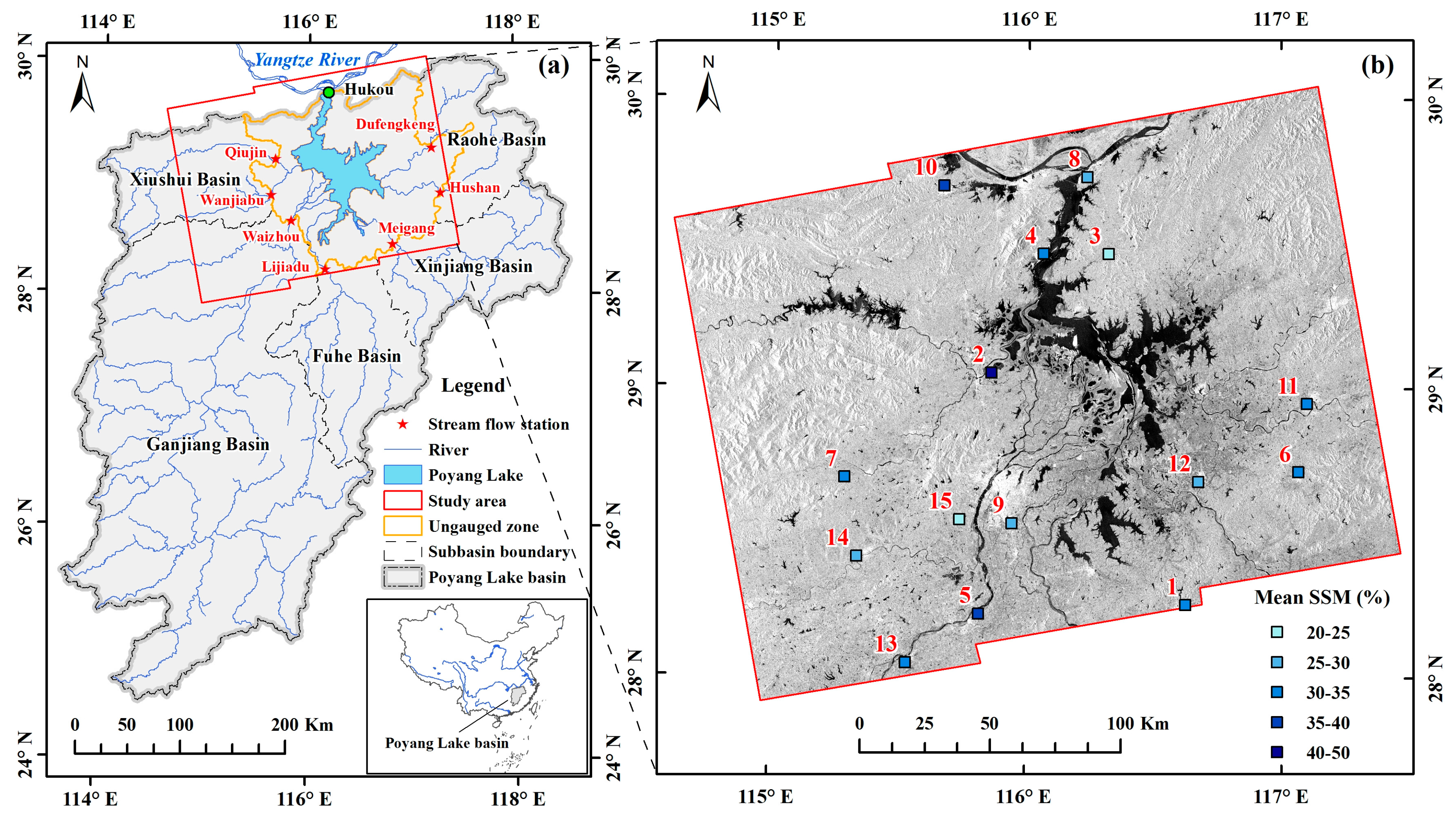
Figure 2.
Scatter plots of measured versus predicted soil moisture from (a) the linear fixed effects model; (b) the mixed effects model without site effect; and (c) the mixed effects model with site effect. The solid black line and dashed red line represent the regression line and 1:1 line, respectively.

Figure 3.
Time series of (a) daily mean temperature and (b) daily accumulated precipitation and measured soil moisture index over Nanchang site (115.9°E, 28.6°N) for the period from April 2015 to December 2016.
Figure 3.
Time series of (a) daily mean temperature and (b) daily accumulated precipitation and measured soil moisture index over Nanchang site (115.9°E, 28.6°N) for the period from April 2015 to December 2016.
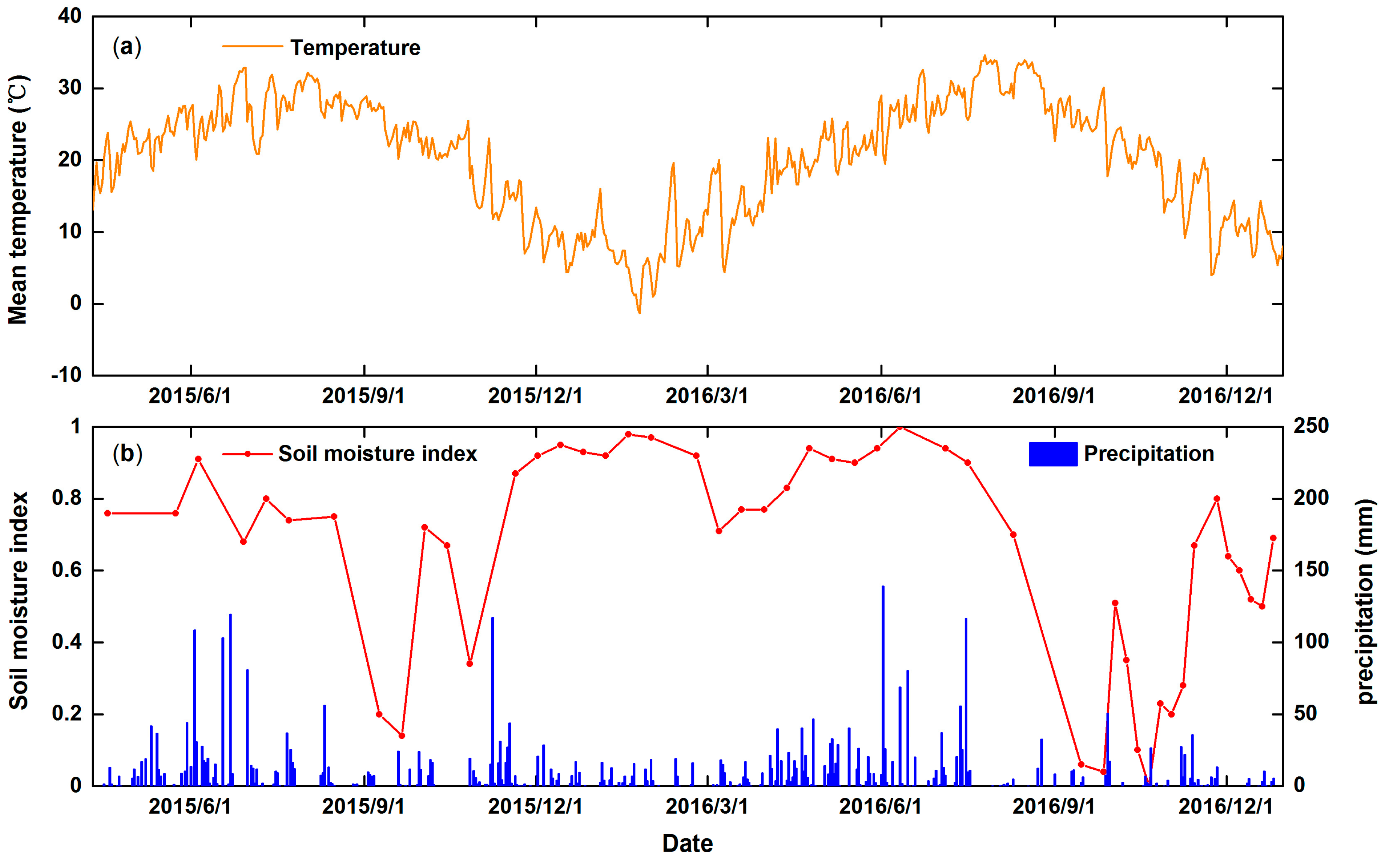
Figure 4.
Measured (black solid lines) and predicted soil moisture indices of 15 observation sites, with the blue dash lines predicted by the linear fixed effects model and the red dash lines predicted by the LME model. Number in lower left corner for each subplot denotes site ID.
Figure 4.
Measured (black solid lines) and predicted soil moisture indices of 15 observation sites, with the blue dash lines predicted by the linear fixed effects model and the red dash lines predicted by the LME model. Number in lower left corner for each subplot denotes site ID.
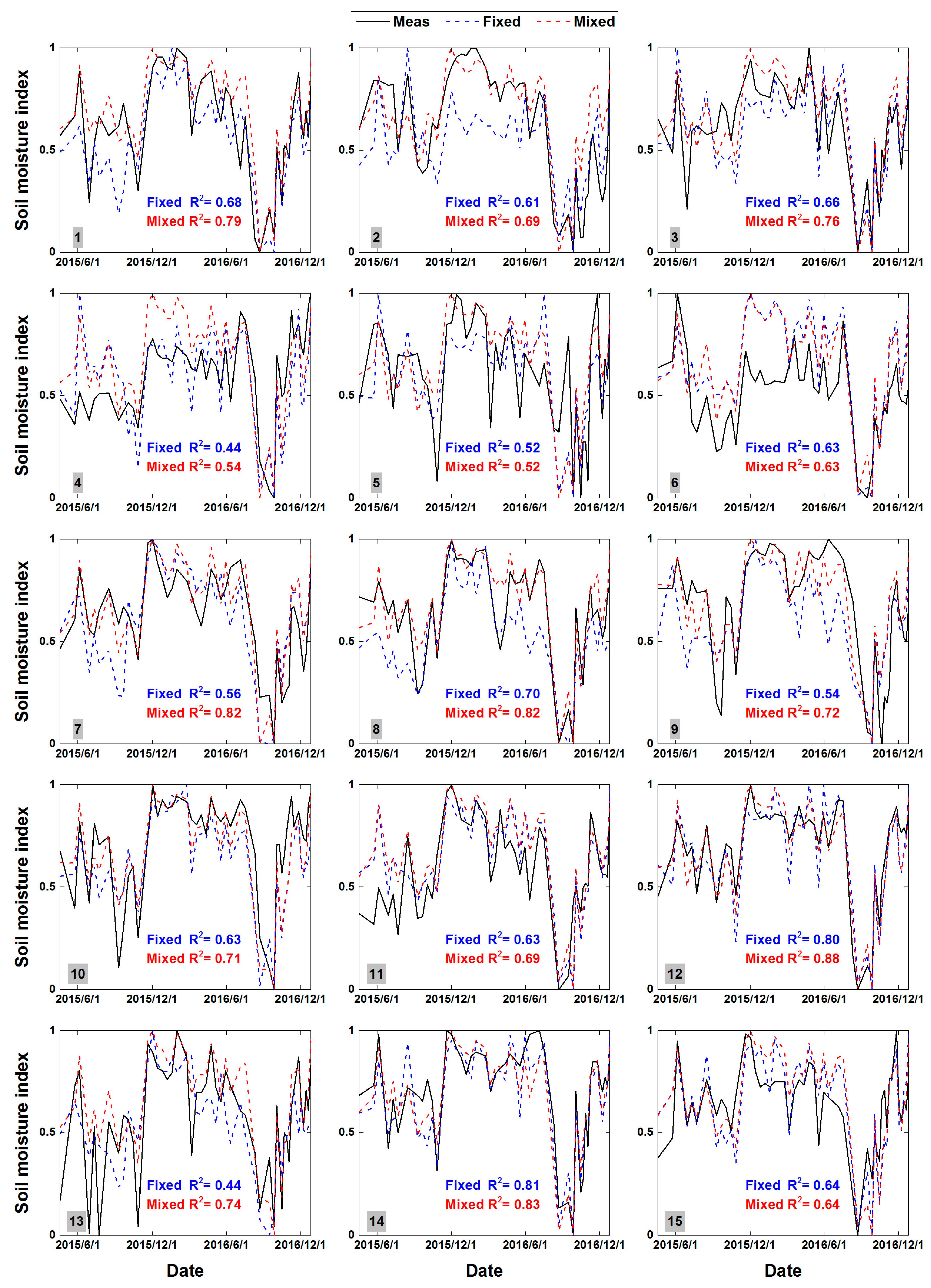
Figure 5.
Scatter plots of measured versus predicted soil moisture indices. (a,c) are model-fitting and cross-validation results for the LME model, respectively; (b,d) are model-fitting and cross-validation results for the linear fixed effects model, respectively. The solid black line and dashed red line represent the regression line and 1:1 line, respectively.

Figure 6.
Relationship between mean soil moisture index and the coefficient of variation (CV). Each point denotes an acquisition and the colors represent different seasons (Spring: MAM; Summer: JJA; Autumn: SON; Winter: DJF).
Figure 6.
Relationship between mean soil moisture index and the coefficient of variation (CV). Each point denotes an acquisition and the colors represent different seasons (Spring: MAM; Summer: JJA; Autumn: SON; Winter: DJF).
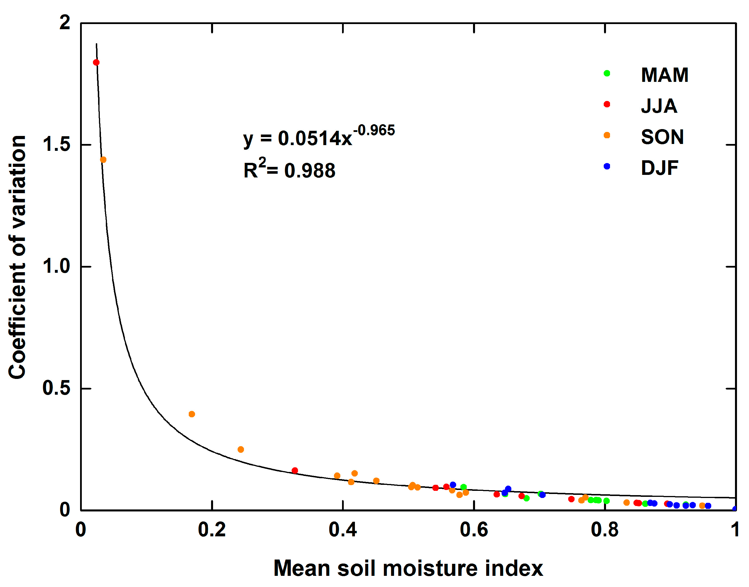
Figure 7.
Soil moisture index maps for six selected dates.

Table 1.
Sentinel-1A/1B acquisitions used in this study.
| Year | Month | Day | ∆days | Sensor |
|---|---|---|---|---|
| 2015 | April | 18 | / | A |
| May | 24 | 36 | ||
| June | 05, 29 | 12, 24 | ||
| July | 11, 23 | 12, 12 | ||
| August | 16 | 24 | ||
| September | 09, 21 | 24, 12 | ||
| October | 03, 15, 27 | 12, 12, 12 | ||
| November | 20 | 24 | ||
| December | 02, 14, 26 | 12, 12, 12 | ||
| 2016 | January | 07, 19, 31 | 12, 12, 12 | A |
| February | 24 | 24 | ||
| March | 07, 19, 31 | 12, 12, 12 | ||
| April | 12, 24 | 12, 12 | ||
| May | 06, 18, 30 | 12, 12, 12 | ||
| June | 11 | 12 | ||
| July | 05, 17 | 24, 12 | ||
| August | 10, 22 | 24, 12 | ||
| September | 15, 27 | 24, 12 | ||
| October | 03, 09, 15, 21, 27 | 6, 6, 6, 6, 6 | B, A, B, A, B | |
| November | 02, 08, 14, 26 | 6, 6, 6, 12 | A, B, A, A | |
| December | 02, 08, 14, 20, 26 | 6, 6, 6, 6, 6 | B, A, B, A, B |
Table 2.
Descriptive statistics of 15 soil moisture observation sites.
| ID | Site Name | Height (m) | Land Cover | Mean (%) | Min (%) | Max (%) | Std. (%) |
|---|---|---|---|---|---|---|---|
| 1 | Dongxiang | 36.6 | Nursery | 33.08 | 23.20 | 39.10 | 3.93 |
| 2 | Yongxiu | 14 | Paddy field | 47.30 | 32.90 | 56.90 | 7.17 |
| 3 | Duchang | 37.7 | Dryland | 20.83 | 4.50 | 31.00 | 5.90 |
| 4 | Xingzi | 62 | Dryland | 30.63 | 16.50 | 39.90 | 4.93 |
| 5 | Fengcheng | 26 | Paddy field | 39.70 | 30.90 | 45.50 | 3.87 |
| 6 | Wannian | 51.7 | Grassland | 30.03 | 19.30 | 40.80 | 4.20 |
| 7 | Fengxin | 75 | Orchard | 30.66 | 24.00 | 34.90 | 2.50 |
| 8 | Hukou | 39.6 | Grassland | 26.81 | 11.30 | 35.80 | 5.95 |
| 9 | Nanchang | 29.9 | Dryland | 27.35 | 20.80 | 30.80 | 2.96 |
| 10 | Ruichang | 23.6 | Dryland | 35.15 | 26.40 | 38.70 | 3.04 |
| 11 | Leping | 26 | Dryland | 30.16 | 22.20 | 35.70 | 3.15 |
| 12 | Yugan | 19 | Dryland | 26.94 | 12.00 | 33.90 | 5.20 |
| 13 | Zhangshu | 29 | Dryland | 32.80 | 27.50 | 36.70 | 2.40 |
| 14 | Gaoan | 34 | Dryland | 27.17 | 19.90 | 30.30 | 2.54 |
| 15 | Xinjian | 7 | Dryland | 20.75 | 13.30 | 24.90 | 2.19 |
Mean, min, max and std. represent mean, minimum, maximum values and standard deviation of soil moisture measurements (0–10 cm) respectively.
Table 3.
The calibrated parameters and performance statistics for three LME models with different polarizations.
Table 3.
The calibrated parameters and performance statistics for three LME models with different polarizations.
| Model | Fixed Slop | Fixed Intercept | Overall R2 | RMSE (%) | MPE (%) |
|---|---|---|---|---|---|
| VV | 0.33 * | 33.36 * | 0.894 | 2.53 | 1.87 |
| VH | 0.13 | 32.54 * | 0.892 | 2.56 | 1.90 |
| VV + VH | VV: 0.34 *; VH: −0.03 | 32.98 * | 0.860 | 3.12 | 2.45 |
* indicates a 0.001 significance level.
Table 4.
Performance statistics for three linear fixed and mixed effects models.
| Model | Temporal R2 | Spatial R2 | Overall R2 | RMSE (%) | MPE (%) |
|---|---|---|---|---|---|
| Fixed | 0.558 | 0.671 | 0.219 | 6.88 | 5.14 |
| Mixed (full) | 0.641 | 1 | 0.894 | 2.53 | 1.87 |
| Mixed (without ) | 0.613 | 0.052 | 0.171 | 7.16 | 5.23 |
© 2017 by the authors. Licensee MDPI, Basel, Switzerland. This article is an open access article distributed under the terms and conditions of the Creative Commons Attribution (CC BY) license (http://creativecommons.org/licenses/by/4.0/).
Share and Cite
MDPI and ACS Style
Zhang, Y.; Gong, J.; Sun, K.; Yin, J.; Chen, X. Estimation of Soil Moisture Index Using Multi-Temporal Sentinel-1 Images over Poyang Lake Ungauged Zone. Remote Sens. 2018, 10, 12. https://doi.org/10.3390/rs10010012
AMA Style
Zhang Y, Gong J, Sun K, Yin J, Chen X. Estimation of Soil Moisture Index Using Multi-Temporal Sentinel-1 Images over Poyang Lake Ungauged Zone. Remote Sensing. 2018; 10(1):12. https://doi.org/10.3390/rs10010012
Chicago/Turabian StyleZhang, Yufang, Jianya Gong, Kun Sun, Jianmin Yin, and Xiaoling Chen. 2018. "Estimation of Soil Moisture Index Using Multi-Temporal Sentinel-1 Images over Poyang Lake Ungauged Zone" Remote Sensing 10, no. 1: 12. https://doi.org/10.3390/rs10010012
Note that from the first issue of 2016, this journal uses article numbers instead of page numbers. See further details here.