Diverse Responses of Vegetation Phenology to Climate Change in Different Grasslands in Inner Mongolia during 2000–2016


1
Institute of Remote Sensing and Geographic Information System, School of Earth and Space Sciences, Peking University, Beijing 100871, China
2
State Key Laboratory of Cryosphere Sciences, Cold and Arid Regions Environmental and Engineering Research Institute, Chinese Academy of Sciences, 320 Donggang West Road, Lanzhou 730000, China
3
School of Geographic Sciences, Nantong University, 999 Tongjing Road, Nantong 226007, China
4
Department of Forest Ecology and Management, Swedish University of Agricultural Sciences, 90183 Umeå, Sweden
5
Key Laboratory of Western China’s Environmental Systems (Ministry of Education), College of Earth and Environmental Sciences, Lanzhou University, Lanzhou 730000, China
*
Author to whom correspondence should be addressed.
Remote Sens. 2018, 10(1), 17; https://doi.org/10.3390/rs10010017
Submission received: 24 October 2017
/
Revised: 13 December 2017
/
Accepted: 21 December 2017
/
Published: 22 December 2017
(This article belongs to the Special Issue Land Surface Phenology )
Abstract
:Vegetation phenology in temperate grasslands is highly sensitive to climate change. However, it is still unclear how the timing of vegetation phenology events (especially for autumn phenology) is altered in response to climate change across different grassland types. In this study, we investigated variations of the growing season start (SOS) and end (EOS), derived from Moderate Resolution Imaging Spectroradiometer (MODIS) data (2000–2016), for meadow steppe, typical steppe, and desert steppe in the Inner Mongolian grassland of Northern China. Using gridded climate data (2000–2015), we further analyzed correlations between SOS/EOS and pre-season average air temperature and total precipitation (defined as 90-day period prior to SOS/EOS, i.e., pre-SOS/EOS) in each grid. The results showed that both SOS and EOS occurred later in desert steppe (day of year (doy) 114 and 312) than in meadow steppe (doy 109 and 305) and typical steppe (doy 111 and 307); namely, desert steppe has a relatively late growing season than meadow steppe and typical steppe. For all three grasslands, SOS was mainly controlled by pre-SOS precipitation with the sensitivity being largest in desert steppe. EOS was closely connected with pre-EOS air temperature in meadow steppe and typical steppe, but more closely related to pre-EOS precipitation in desert steppe. During 2000–2015, SOS in typical steppe and desert steppe has significantly advanced by 2.2 days and 10.6 days due to a significant increase of pre-SOS precipitation. In addition, EOS of desert steppe has also significantly advanced by 6.8 days, likely as a result from the combined effects of elevated preseason temperature and precipitation. Our study highlights the diverse responses in the timing of spring and autumn phenology to preceding temperature and precipitation in different grassland types. Results from this study can help to guide grazing systems and to develop policy frameworks for grasslands protection.
1. Introduction
Vegetation phenology is the study of periodic biological events in the plant world and their relations with environmental factors, such as air temperature and rainfall [1,2]. As vegetation phenology controls the mass and energy exchanges between terrestrial ecosystems and the atmosphere [3,4,5,6], accurate monitoring of vegetation phenology is crucial to assess the interactions between vegetation dynamics and climate change [7,8]. In the past decades, vegetation spring phenology has attracted a great deal of attention due to its close connection with global change. In contrast, understanding of vegetation autumn phenology is limited, though it can play an important role in determining vegetation growing season length and has been found to be significantly affected by climatic change [9].
Ground-observed phenological data and satellite data are two major tools commonly used to identify vegetation growing season at different scales. Ground data are commonly recorded at the species level and used for conducting species-specific phenology analysis at local scales [10,11,12,13]. Meanwhile, satellite data are mainly employed to define the growing season characteristics of entire landscapes at regional to global scales [14,15,16,17,18,19]. Various satellite-derived vegetation indices have been developed to extract vegetation phenological metrics, such as the Normalized Difference Vegetation Index (NDVI) and the Enhanced Vegetation Index (EVI) [20,21,22,23]. Most studies, however, have focused on the spatiotemporal differences of phenological events among diverse biomes or geographic zones [19,24,25,26]. In contrast, only few attempts exist on revealing how vegetation phenology responds to climate change for different vegetation types within a given biogeographic zone at the regional scale.
Grassland is a widely distributed vegetation type around the world and plays an important role in providing resources to humankind, supplying feed for animals, and maintaining stability of ecological systems globally [27]. However, plant growth in grassland ecosystems is highly sensitive to regional and global climate change. Several studies have reported higher temporal variations in spring phenology of herbaceous species compared to woody plants and described their complex and controversial response to climate change in temperate grasslands [13,28,29,30]. Most previous studies suggest that a warmer spring results in an advancement of spring phenological events of grassland vegetation [11,31,32,33,34]. However, under conditions where concurrent precipitation is limiting, increasing temperature may have no significant effects on spring phenology [35,36]. It has been shown that increasing precipitation had no significant effects on flowering dates in two temperate grasslands of North America [37,38], while reduced precipitation induced an earlier green-up and flowering of herbaceous species in field experiments [39,40,41]. The distinct responses of spring phenology events to climate change in grassland ecosystems may be closely coupled with vegetation types [42]. Our knowledge of the controls regulating autumn phenology of different vegetation types in grassland ecosystems is, however, currently limited. Given the potential differences in climate change impacts, it is crucial to improve our understanding with regard to the responses of both spring and autumn phenological events to climate change among different grassland types.
Transhumance provides livestock access to green vegetation during the short periods of active growth in each place. It distributes livestock grazing pressure and lengthens the time period when livestock have access to quality forage [43]. Thus, the transhumance system is closely connected with vegetation phenology. Different vegetation phenology in space not only determines the spatial difference of timing of plant growth [44], but also leads to the spatial heterogeneity of nutritional parameters of pastures [45,46]. Those spatial gradients caused by phenology do influence the timing and direction of transhumance movements. Therefore, studying phenology and its relationships with primary meteorological factors would help pastoralists and rangeland managers to reasonably develop strategies to conduct grazing activities and avoid overgrazing in local places in perspective of sustainable usage of pastures.
In this study, we first derived the start (SOS) and end (EOS) of growing season from Moderate Resolution Imaging Spectroradiometer (MODIS) data (2000–2016) for three grassland types in the Inner Mongolian grassland of Northern China, i.e., meadow steppe, typical steppe, and desert steppe. Then, we tested their reliability be means of SOS/EOS retrieved from ground-measured gross primary production (GPP) data. Finally, combined with gridded climate data, we analyzed the differences of SOS/EOS response to previous temperature and precipitation among the three grassland types. The main objectives of this study were to address the following scientific questions: (i) Are there significant differences in the timing of SOS and EOS among the three grassland types? (ii) What climate factor mainly controls SOS and EOS dynamics for the whole Inner Mongolian grassland? (iii) Are there any differences of SOS and EOS responses to climate changes among the three grassland types? (iv) Are there significant trends in the SOS and EOS during 2000–2016 in the three grassland types? What climate factors primarily contribute to them?
2. Materials and Methods
2.1. Study Region
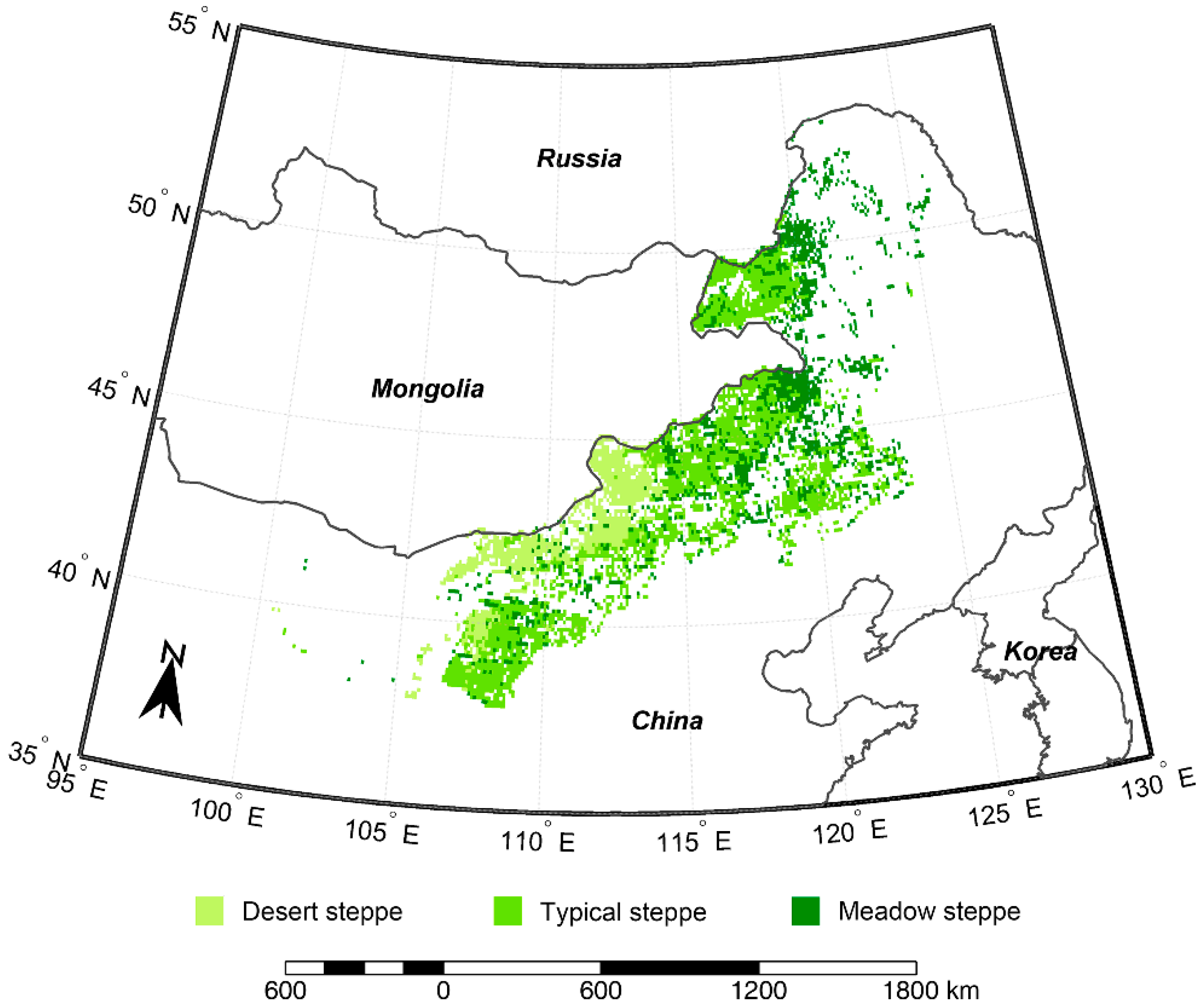
The Inner Mongolian grassland is situated in the northern part of China, with an elevation ranging 1000–2000 m above sea level. This region is characterized by a temperate continental monsoon climate, with a cold-dry winter and a hot-moist summer. The annual mean air temperature increases from −3.9 °C in the northeast to 10 °C in the southwest. The annual mean total precipitation decreases from 466 mm in the east to 42 mm in the west [47]. Herbaceous plants are dominating vegetation types in this region. Meadow steppe (29.4% of total areas, 2.3 × 10⁷ ha), typical steppe (52.8%, 4.2 × 10⁷ ha), and desert steppe (17.8%, 1.4 × 10⁷ ha) were classified in this study (Figure 1), which were defined by the 1:1,000,000 Editorial Board of Vegetation Map of China according to geomorphological features, climate conditions, soil types, and dominant species [48]. Forests and deserts were not included in this study.
2.2. Remote Sensing Data and Processing
Moderate Resolution Imaging Spectroradiometer (MODIS) datasets have been extensively used to explore large-scale phenology making use of their high quality and richness of available products. In this study, MODIS Surface Reflectance 8-Day L3 Global 500 m product (MOD09A1) during 2000–2016, acquired from the Oak Ridge National Laboratory Distributed Active Archive Center (ORNL DAAC) (https://search.earthdata.nasa.gov/search), was used to calculate NDVI (Equation (1)):
where Band 1 and Band 2 denote the reflectance values of red (620–670 nm) and near-infrared (841–876 nm), respectively. This NDVI product is derived from eight-day maximum value composites by choosing observations with minimal cloud cover and near-nadir views [49]. Further corrections for atmospheric gases, clouds, and aerosols have been routinely applied [50].
Although the highest-quality reflectance values have been selected, some poor quality values may still exist due to prolonged rainfall and cloudy weather periods. Eliminating these abnormal values in NDVI time series is of crucial importance to obtain credible phenological metrics. Usually, there are some sequential abnormal low points occurring at the start and end of the time series, and a few abrupt and extreme low points were observed in the middle of growing season (Figure 2a). We first addressed the issue of abrupt points [NDVI (t)] in the middle of the growing season. If the difference between NDVI (t) and NDVI (t ± 1) is larger than (NDVImax − NDVImin)/2, NDVI (t) was replaced by the average value of NDVI (t − 1) and NDVI (t + 1). Then, we smoothed the entire time series with a nine-point moving average filter. Finally, abnormally low values at the start and end of the time series were replaced with the average NDVI value in March, when most NDVI values are approximately equal to the NDVI value of bare ground due to a lack of vegetation activities and little snow on the surface. Here, we assumed that the NDVI values during the non-growing season are approximately constant.
Several methods have been developed to extract phenological information from NDVI curves [51,52]. Among them, the logistic function can accurately simulate the growth process of vegetation and fit NDVI curves, and has been employed by National Aeronautics and Space Administration (NASA) to produce MODIS global vegetation phenology products [14]. The typical logistic function retrieves phenological metrics during spring and autumn separately, while the double logistic function can extract spring and autumn phenological events simultaneously [44,53,54,55]. In this study, therefore, the reconstructed NDVI time series were fitted using double logistic function (Equation (2)) to obtain SOS and EOS based on Equations (3) and (4), respectively:
where NDVI (t) is the reconstructed NDVI values at time t; NDVImax and NDVImin are the maximum and minimum values in the NDVI time series, respectively; I and D represent the maximum rising and falling slopes (inflection points) on the fitted NDVI curve; and S and E represent corresponding dates of I and D on the fitted NDVI curve. In this study, SOS/EOS was defined as the date corresponding to the first/last local maximum/minimum changing rate of curvature (Figure 2a) [54]. For simplicity, we taken the middle day of each eight-day compositing window as the ‘real’ date in which the NDVI value was obtained. Additionally, pixels with an annual amplitude of NDVI less than 0.1 and two growing seasons were not considered in this study. All data processing was fulfilled with the MATLAB software (Matlab R2016a, MathWorks Inc., Natick, MA, USA).
2.3. Gross Primary Production Data
Validation of remotely-sensed phenological metrics is usually a necessary step before using them for further analysis. However, manual records of phenophases only represent the development status of an individual of a specific species and may be not suitable to validate the accuracy of remotely-sensed phenological metrics, which directly reflects the growth conditions of a local community. In comparison, GPP data measured in eddy covariance flux sites could reflect the overall dynamics of the local community and has been widely used in land surface phenology validation for different biomes [26,56]. Thus, we validated the accuracy of remotely-sensed SOS/EOS by directly comparing them with GPP-based SOS/EOS in six site-years (Table 1). GPP data were collected from the FLUXNET2015 dataset (http://fluxnet.fluxdata.org/) and two published literatures [57,58]. GPP-based SOS/EOS was also obtained by using the double logistic function to fit GPP time series in each site-year (Figure 2b).
2.4. Climate Data
In this study, a gridded China Meteorological Forcing Dataset (http://dam.itpcas.ac.cn/chs/rs/?q=data) was used for exploring the relations between SOS/EOS and dominating climate factors, which was developed by Data Assimilation and Modeling Center for Tibetan Multi-spheres, Institute of Tibetan Plateau Research, Chinese Academy of Sciences [59,60]. It includes seven three-hourly climate variables from 2000 to 2015 at a spatial resolution of 0.1° × 0.1°. In this current study, however, because SOS/EOS changes are primarily correlated with the hydrothermal conditions of the previous 2–3 months [31,33,43], and the effects of sunlight on herbaceous plants are relatively weak [8,61,62], only the temperature and precipitation rate were employed. In order to match the temporal resolution of phenological metrics, we calculated daily air temperature and precipitation from the three-hourly air temperature and precipitation data, respectively. We verified that the gridded temperature and precipitation could accurately characterize the ground hydrothermal variations by comparing them with the measured data at 42 national meteorological stations during 2000 to 2011 (Table S1), which were acquired from the China Meteorological Administration.
2.5. Data Analysis
In this study, we first analyzed spatial patterns of SOS/EOS and compared SOS/EOS differences among meadow steppe, typical steppe, and desert steppe with one-way analysis of variance (ANOVA). The accuracy of MODIS-based SOS/EOS was assessed with R2 (goodness of fit) and RMSE (root mean square error) by regressing them with GPP-based SOS/EOS.
Secondly, we calculated the Pearson correlation coefficient between SOS/EOS and pre-season average temperature/total precipitation (defined as 90-day and 60-day before multi-year average SOS/EOS) in each grid. As 90-day and 60-day results were similar, we only presented the former in this study. For clearly distinguishing, the 90-day periods prior to SOS and EOS were named as ‘pre-SOS’ and ‘pre-EOS’, respectively. Finally, we established linear regression models to obtain the sensitivity of SOS/EOS to temperature/precipitation in each grid. One-way ANOVA was taken to compare the sensitivity of SOS/EOS to these main climatic variables among the different vegetation types. It is worth noting that regression analysis between SOS/EOS and climate factors only covers the period of 2000–2015 (data for 2016 was not available). When conducting regression analyses between SOS/EOS and climate factors, we used the average SOS/EOS of all pixels falling in a climate grid.
The variation trends analysis of SOS/EOS was conducted in both pixel scale and vegetation type scale. In pixel scale, variation trends of SOS/EOS during 2000–2016 were computed with the Theil-Sen median method in each pixel, which chooses the median of the slopes of all lines through pairs of two-dimensional sample points. The non-parametric Mann-Kendall test was employed to assess the significance of trends. Compared with linear regression, the Theil-Sen median method is more robust and not affected by outliers.
In vegetation type scale, however, we chose to directly compare SOSs/EOSs in the head and tail of the studying period instead of computing trends of multi-pixel average SOS/EOS, with the aim to reduce calculation errors. To eliminate the effects of SOS/EOS in possibly abnormal years, we first obtained multi-year average SOS/EOS during 2000–2004 and 2011–2015 in each pixel. We then compared the overall SOS/EOS differences between 2000–2004 and 2011–2015 with two-sample t-test in meadow steppe, typical steppe, and desert steppe separately. Meanwhile, for investigating the possible reasons that resulted in SOS/EOS variations, we also analyzed the variations of pre-SOS/EOS temperature and precipitation from 2000–2004 to 2011–2015 with the same methods in each of the three grassland types, respectively. Notably, the significance of all statistical analyses in this study were tested at the 95% level (i.e., p = 0.05).
3. Results
3.1. Environmental Conditions
The multi-year (2000–2015) averages of environmental conditions showed that spring temperature in desert steppe was higher than in meadow steppe and typical steppe, whereas the spring precipitation in desert steppe was lower compared with that in meadow steppe and typical steppe. In autumn, desert steppe was also warmer and drier than meadow steppe and typical steppe. During both spring and autumn, meadow steppe was the coldest and wettest among the three grassland types. For all the three grassland types, autumn was colder and wetter than spring (Table 2).
3.2. Ground Validation
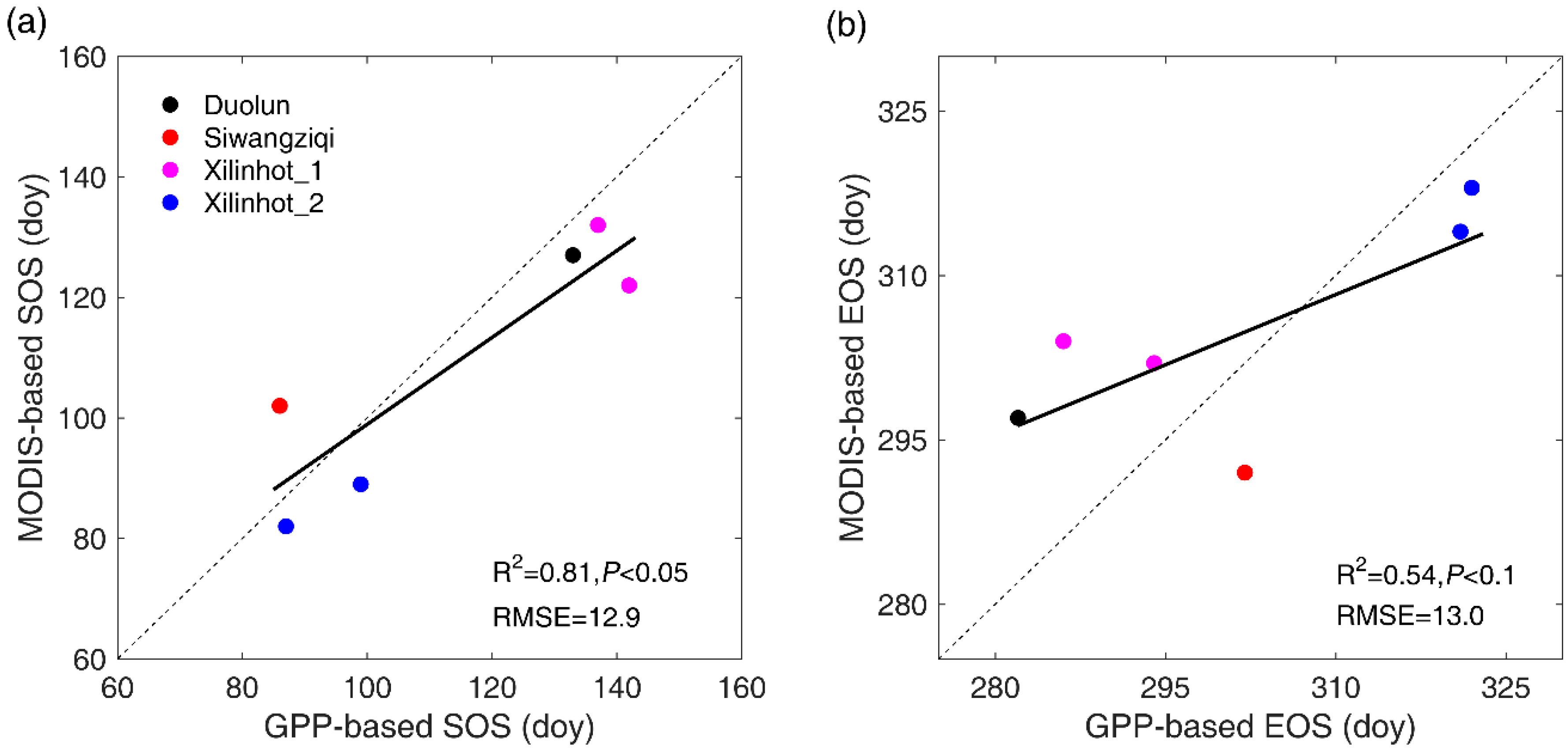
Figure 3 illustrated a significant and positive correlation between MODIS-based SOS and GPP-based SOS (p < 0.05), and between MODIS-based EOS and GPP-based EOS (p < 0.1). The mean estimation error of MODIS-based SOS was 12.9 days, with the smallest error (five days earlier than GPP-based SOS) detected in 2003 at Xilinhot_2 and in 2004 at Xilinhot_1, and the largest gap (20 days earlier than GPP-based SOS) found in 2006 at Xilinhot_1. The estimation errors of MODIS-based EOS range from four days (in 2003 at Xilinhot_2) to 18 days (in 2006 at Xilinhot_1), with an average of 13.0 days.
3.3. Overall SOS/EOS Comparison among the Three Grassland Types
For the entire study region, SOS occurred mainly in April and May at an average day of year (doy) of 111 and EOS appeared mainly in October and November (doy 307). Spatially, SOS occurred earlier in the northeast than in the southwest and southeast (Figure 4a). A strong spatial gradient of EOS was noted suggesting a delay from northeast towards southwest (Figure 4b). In terms of different grassland types, SOS and EOS in meadow steppe (doy 109 and 305) both occurred significantly earlier than in typical steppe (doy 111 and 307) and desert steppe (doy 114 and 312) for several days (Figure 4c,d). Meanwhile, SOS and EOS in typical steppe also occurred slightly, but significantly earlier than in desert steppe. This suggests a similar growing season length of vegetation among meadow steppe (196 days), typical steppe (196 days), and desert steppe (197 days). As to inter-annual fluctuations of SOS and EOS, our results revealed that the mean standard deviation (SD) of EOS (9.5 days) was smaller than that of SOS (15.5 days). The greatest SDs of SOS and EOS were both found in desert steppe (23.3 and 11.3 days) when compared with that in meadow steppe (11.5 and 9.2 days) and typical steppe (15.1 and 9.1 days).
3.4. Correlations between SOS/EOS and Temperature/Precipitation
In order to identify which factor determines the timing of SOS/EOS, we analyzed the correlations of SOS/EOS with pre-SOS/pre-EOS temperature and precipitation. Figure 5a,b showed that significant negative and positive correlations between SOS and pre-SOS temperature both occurred in 1.2% of pixels. Meanwhile, SOS was significantly negatively correlated with pre-SOS precipitation in 12.9% of pixels while significant positive relationships between SOS and pre-SOS precipitation were only found in 0.1% of pixels. Similarly, a significant negative correlation between SOS and pre-SOS precipitation was found in 13.2% of meadow steppe pixels, 13.2% of typical steppe pixels, and 11.3% of desert steppe pixels. Meanwhile, significant negative correlations between SOS and pre-SOS temperature were only detected in 3.5% of meadow steppe pixels, 0.2% of typical steppe pixels, and 0.2% of desert steppe pixels.
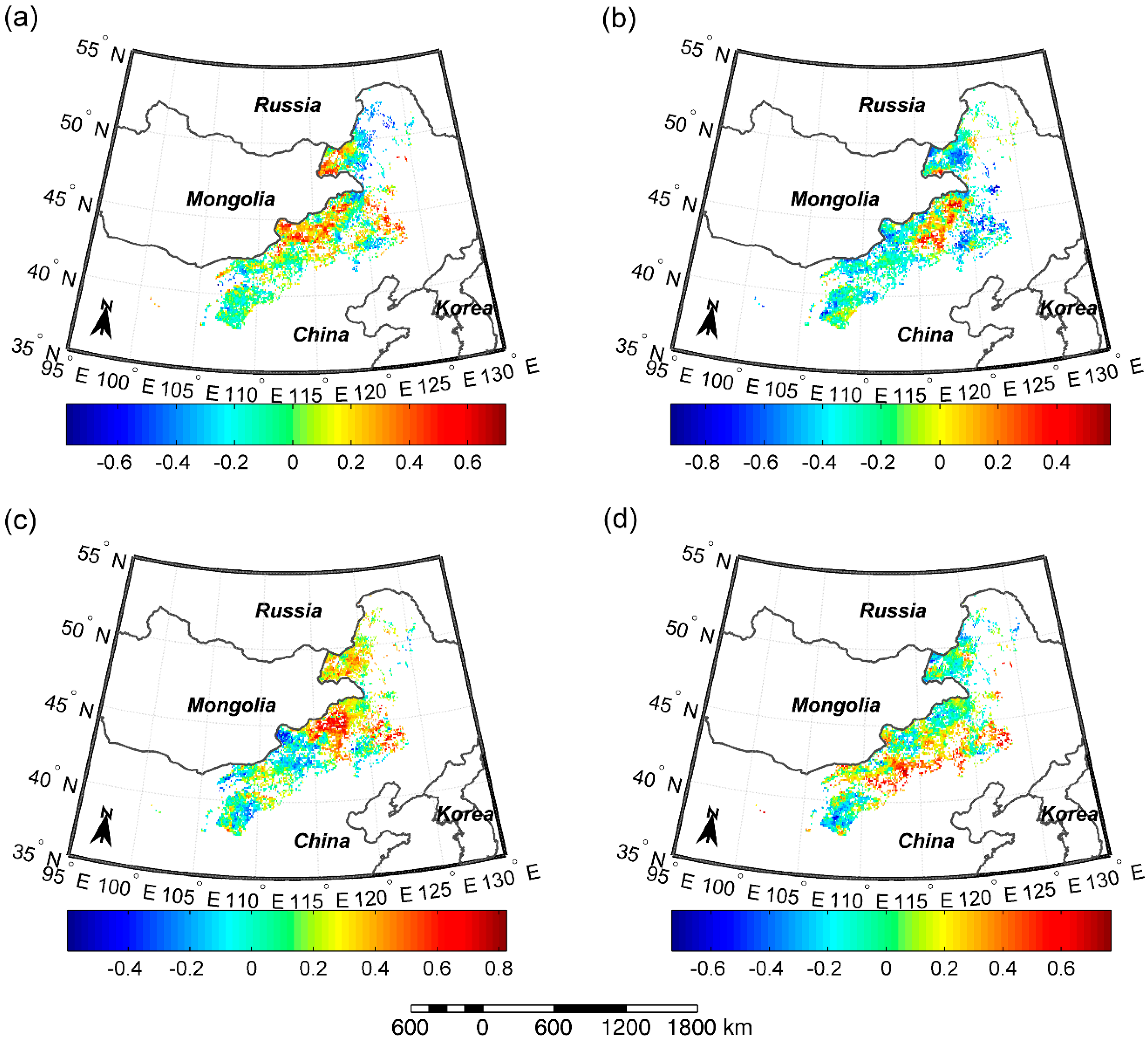
In contrast to SOS, significant positive correlations were detected between EOS and pre-EOS temperature in 8.8% of total pixels, and between EOS and pre-EOS precipitation in 3.8% of total pixels (Figure 5c,d). Significant negative correlations between EOS and pre-EOS temperature/precipitation were found only in few pixels (0.1%/0.3%). Moreover, significant positive relationships were discovered between EOS and pre-EOS temperature/precipitation in 9.8%/3.5% of meadow steppe pixels and 11.1%/4.8% of typical steppe pixels. In desert steppe, significant positive correlations were found between EOS and pre-EOS precipitation in 1.0% of pixels, while no significant positive relationships were found between EOS and pre-EOS temperature.
3.5. Response Rates of SOS/EOS to Temperature and Precipitation
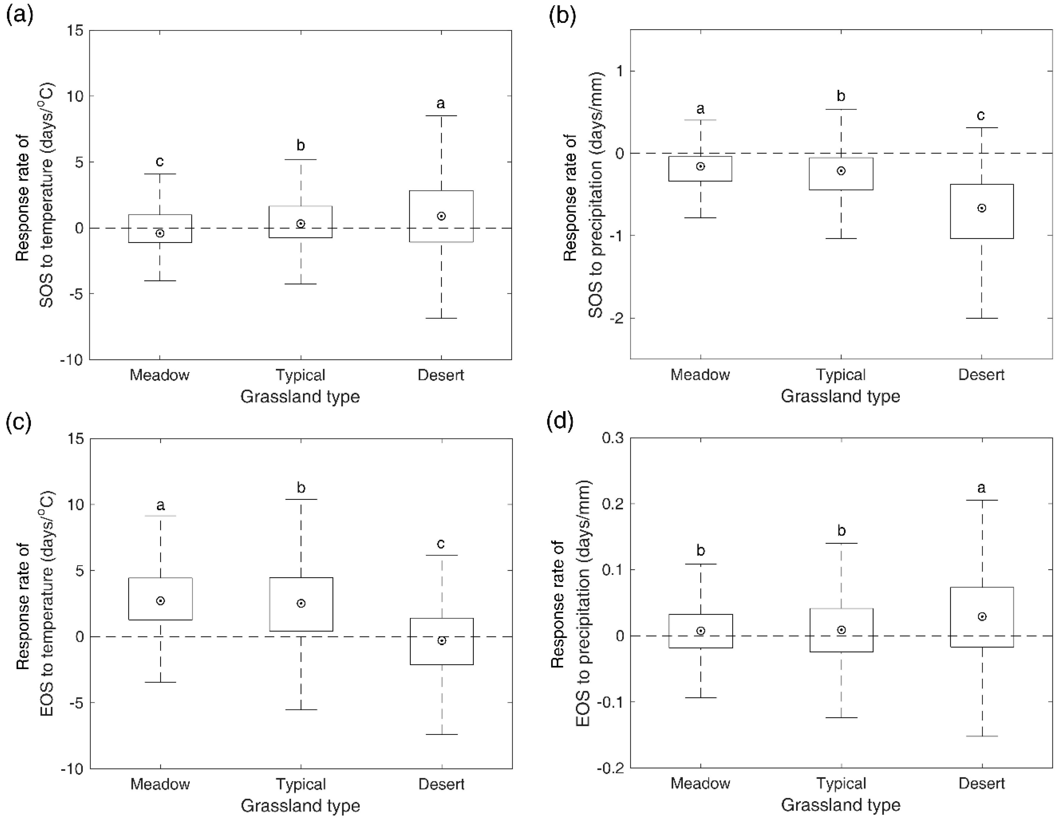
During 2000–2016, we observed an advancement of 0.41 days/°C for SOS in meadow steppe, and a delay of 0.33 and 0.9 days/°C for SOS in the typical and desert steppe (Figure 6a). Meanwhile, increased spring pre-SOS precipitation caused an advance in SOS by 0.16, 0.21, and 0.66 days/mm for meadow steppe, typical steppe, and desert steppe, respectively (Figure 6b). The sensitivity of SOS to pre-SOS temperature and precipitation in desert steppe was significantly stronger than that in meadow steppe and typical steppe. In autumn, warmer temperatures delayed EOS at rates of 2.71 and 2.51 days/°C for meadow steppe and typical steppe, whereas they advanced EOS by 0.31 days/°C for desert steppe (Figure 6c). Increased precipitation caused a delay in the timing of EOS by 0.01, 0.01, and 0.03 days/mm for meadow steppe, typical steppe, and desert steppe, respectively (Figure 6d). Desert steppe showed a significantly weaker sensitivity of EOS to pre-EOS temperature, but a significantly stronger sensitivity of EOS to pre-EOS precipitation than meadow steppe and typical steppe.
3.6. Variation Trends of SOS and EOS
Across the whole study region, a significant advancing trend of SOS was found over the 2000–2016 period in 2.8% pixels and only 0.4% of pixels presented a significant delaying trend (Figure 7a). For meadow steppe, typical steppe, and desert steppe, alone, we also found a higher number of pixels showing a significantly advancing trend (1.8%, 3.9%, 1.2%) compared to the number of pixels showing a significantly delaying trend (0.5%, 0.4%, 0%) (Figure 7c). For EOS, 1.8%/1.6% of pixels showed significant delaying/advancing trends over the whole study region (Figure 7b). In terms of different grassland types, significant advancing trends were detected in 1.7%, 0.8%, and 3.9% of pixels and significant delaying trends were identified in 1.9%, 2.2%, and 0.2% of pixels for meadow steppe, typical steppe, and desert steppe, respectively (Figure 7d).
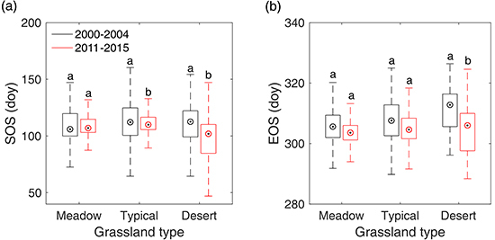
In order to reveal the overall changes of SOS/EOS in the three grassland types, we further compared the multi-year average SOS/EOS during 2000–2004 and that during 2011–2015 with a two-sample t-test in meadow steppe, typical steppe, and desert steppe, respectively. The results illustrated that SOS and EOS did not show a significant trend from 2000–2004 to 2011–2015 in meadow steppe (Figure 8). In typical steppe, SOS have advanced by 2.2 days, while EOS presented no significant changes from 2000–2004 to 2011–2015. In desert steppe, however, we identified a significant advancement for both of SOS and EOS from 2000–2004 to 2011–2015. In 2011–2015, SOS and EOS occurred earlier by 10.6 days and 6.8 days than that in 2001–2004, respectively.
4. Discussion
4.1. Explanation of the Overall Differences of SOS/EOS among Different Grassland Types
Our results suggest that both SOS and EOS occurred later in desert steppe than in meadow steppe and typical steppe. This implies that the growing season in desert steppe is shifted posterior compared to the other two types of steppes. The delayed plant growth for desert steppe in spring may result from the relative shortage of water, although the higher temperature in spring facilitates meeting the thermal requirements needed for vegetation growth. However, the latest EOS detected in desert steppe might be due to higher temperature and the absence of water constraints in autumn. Similarly, the earliest SOS in meadow steppe may result from sufficient water supply in spring, while the earliest EOS could be triggered by the colder weather than typical steppe and desert steppe (Table 1). In addition, the smaller SD in EOS than in SOS suggests that the timing of autumn phenological events are more stable compared with spring phenological events in Inner Mongolian grasslands. Meanwhile, the larger SDs of SOS and EOS in desert steppe indicate a stronger fluctuation of phenological events compared to meadow steppe and typical steppe.
4.2. Key Factors of Controlling SOS/EOS for the Whole Study Region
In this study, we found that SOS was significantly and negatively correlated with pre-SOS precipitation and temperature in most places within the study region. This means that a warmer and wetter pre-SOS period both could cause advanced plant growth. However, considerably more pixels showed significant correlations between SOS and pre-SOS precipitation than that between SOS and pre-SOS temperature. This suggests that water availability rather than temperature mainly controls the timing of vegetation green-up in most parts of Inner Mongolian grasslands. This is, to some extent, in line with the results of two similar studies based on satellite-derived green-up date and ground meteorological data [47,63]. Some process-based phenology modelling and experimental studies have also previously highlighted the critical effects of water availability on SOS in North American grasslands [11,18] and Inner Mongolian grasslands [64,65]. In contrast, however, temperature has been reported as key factor of determining spring phenological events of woody plants in temperate ecosystems [66], and herbaceous species in alpine ecosystems [67].
Similarly, the larger number of pixels showing significant positive correlations between EOS and pre-EOS temperature than that between EOS and pre-EOS precipitation, indicates that temperature may be the more important factor than precipitation in regulating vegetation autumn phenology in temperate grasslands. However, although temperature was the dominant driver, precipitation was also positively related with EOS. Overall, warmer and wetter autumn conditions therefore would lead to a delay of the leaf senescence process. The predominant role of temperature in affecting EOS has also been observed in Mongolian grasslands [68] and in the Tibetan Plateau [69]. However, other studies reported precipitation to be more important than temperature in determining autumn phenology of temperate grassland ecosystems [47,62]. The discrepant conclusion among different studies may be related to differences in data sample size and acquisition methods, as well as in spatial and temporal scales, but also in the studied vegetation types.
4.3. Response of SOS/EOS to Climate Change among Different Grassland Types
We observed that SOS had a similar response to pre-SOS precipitation but different response to pre-SOS temperature among meadow steppe, typical steppe, and desert steppe. Our results suggest that enhanced pre-SOS rainfall could advance vegetation green up in all the three grassland types. A greater pre-SOS temperature may advance SOS in meadow steppe given sufficient water supply from thawed frozen soil which may store substantial amounts of water from the previous winter [70,71]. In contrast, a rapid temperature increase in spring would delay SOS in typical steppe and desert steppe due to the concurrent rapid increase in evaporation and sharp decrease in soil moisture supply [68]. The better relationship between SOS with pre-SOS precipitation than temperature illustrates that SOS is primarily controlled by water regime in all the three grassland types. This agrees with previous results reported by Zhu and Meng [63].
Similar to SOS, the effects of pre-EOS precipitation on EOS in meadow steppe, typical steppe, and desert steppe were concordant. Based on these results, increased pre-EOS precipitation would delay the end of vegetation growing season in all the three grasslands types. However, EOS in desert steppe was more sensitive to moisture dynamics than that in meadow steppe and typical steppe. Similarly, like SOS, the response of EOS to pre-EOS temperature was discrepant among the three grassland types. Our results suggest that higher pre-EOS temperature may delay the end of plant growth in meadow steppe and typical steppe, while terminating the vegetation growing season earlier in desert steppe. Based on our findings, we conclude that temperature mainly determines vegetation autumn phenology in meadow steppe and typical steppe, whereas precipitation is the main driver of vegetation autumn phenology in desert steppe.
Furthermore, the sensitivity of SOS/EOS to pre-SOS/pre-EOS temperature and precipitation changes varied among meadow steppe, typical steppe, and desert steppe. SOS in desert steppe showed the highest sensitivity to both pre-SOS temperature and precipitation than meadow steppe and typical steppe, which is in accordance with the results reported in the same region by Yu et al. [42]. Meanwhile EOS in meadow steppe and typical steppe exhibit a stronger sensitivity to pre-EOS temperature, but weaker sensitivity to pre-EOS precipitation than desert steppe, as previously suggested by Yang et al. [72]. The greater SD of SOS/EOS found in desert steppe than that in meadow steppe and typical steppe observed in our study was also found in the study by Yu et al. [73], suggesting a more complex and sensitive vegetation growth pattern in desert ecosystems.
4.4. What Factors Contributed to SOS/EOS Trends
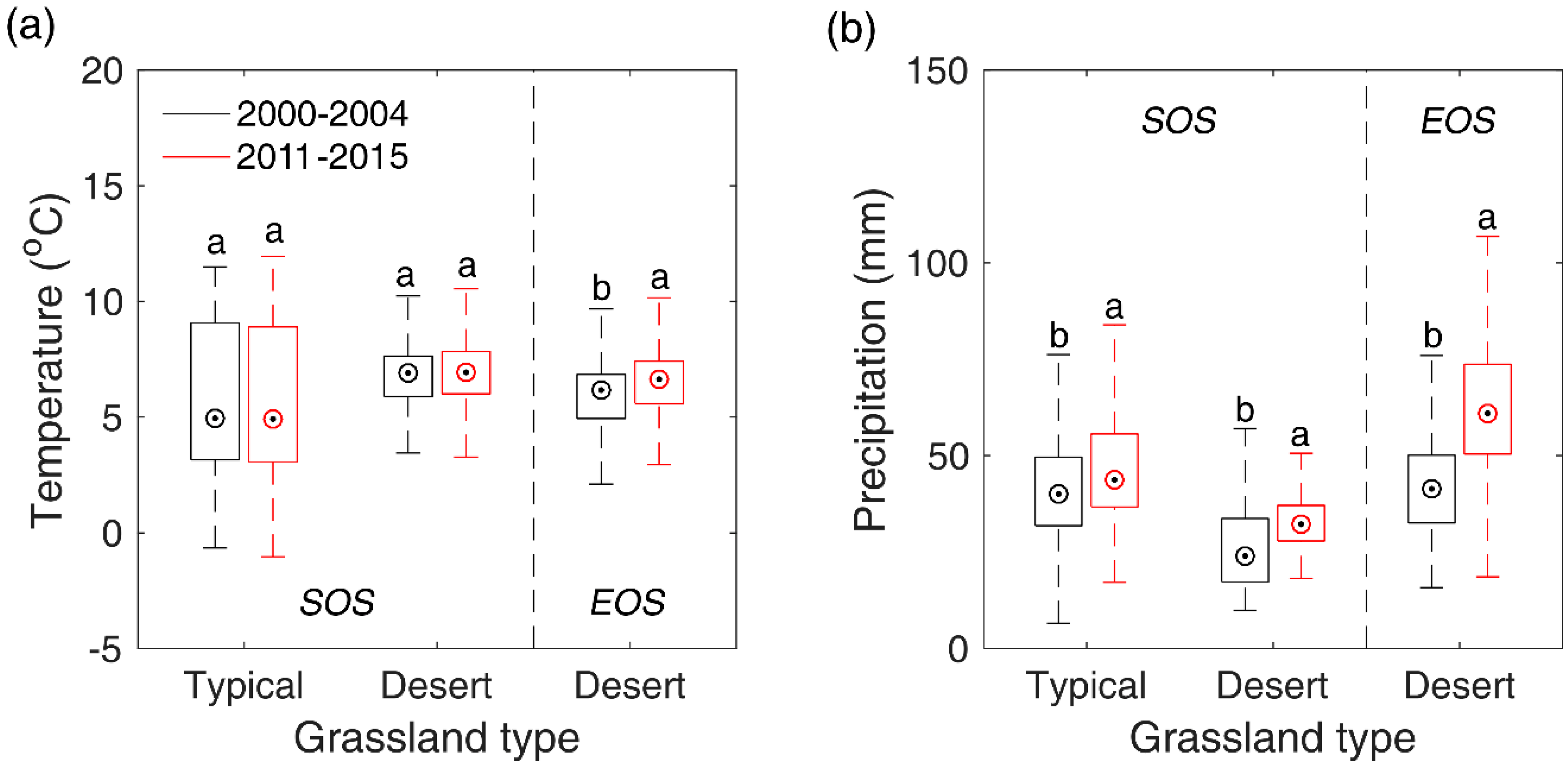
Though our study detected only few of pixels (<4.0% of total pixels) showing significant SOS/EOS trends during 2000–2016 in Inner Mongolian grasslands. However, by comparing the multi-year mean SOS/EOS of 2000–2004 and that of 2011–2015, we still found a significant advance of SOS in typical steppe and desert steppe, and a significant advance of EOS in desert steppe, which have also been identified by other studies with different data and methods [62,74]. SOS experienced a larger shift than EOS. This may, again, indicate that SOS is more sensitive to climate changes than EOS in temperate grasslands. To explore what factor likely contributed to SOS/EOS trends in the two steppes, we compared the differences of the multi-year mean pre-SOS temperature and precipitation between 2000–2004 and 2011–2015 with a two-sample t-test. Results showed that the significant advance of SOS in typical steppe and desert steppe may both result from the pre-SOS significant increase of precipitation (8.6 mm for typical steppe and 6.7 mm for desert steppe), while pre-SOS temperature showed no significant changes from 2000–2004 to 2011–2015 (Figure 9). This is likely due to the negative influence of precipitation on SOS in typical steppe and desert steppe which has been revealed in Section 3.5, namely, more precipitation in preseason would advance the occurrence time of SOS. In comparison, the significant advancement of EOS occurred in desert steppe may stem from the combined effects of the significant elevation of pre-EOS temperature and precipitation. Though the precipitation has increased by 15.4 mm from 2000–2004 to 2011–2015, the significantly boosted temperature (0.77 °C) may accelerate the evaporation of land surface and lead to more water loss and an earlier EOS.
4.5. The Limitation and Implication of This Study
In this study, we validated the reliability of remotely-sensed SOS/EOS with eddy-observed GPP data in typical steppe and desert steppe. The significant and positive correlations between remotely-sensed SOS/EOS and GPP-based SOS/EOS indicate the remotely-sensed SOS/EOS could reflect spatiotemporal dynamics of ground vegetation phenology to some extent. Nevertheless, there are still some gaps between remotely-sensed SOS/EOS and GPP-based SOS/EOS, which may result from the different spatial scales. Another limitation of the validation is the lack of sufficient ground measured data, especially in meadow steppe. Therefore, the results and conclusions of this study need to be further tested with more extensive ground data sources.
This study revealed a diverse response of vegetation phenology to climate change in meadow steppe, typical steppe, and desert steppe, which may indicate different succession directions and spatial patterns of them under the more complex future climate changes. The overall stronger sensitivity of SOS/EOS to hydrothermal conditions identified in desert steppe means plant activity in desert steppe is more unstable than that in meadow steppe and typical steppe. As detected, the whole growing season in desert steppe has significantly advanced and prolonged due to significant climate changes in the past 17 years. This could lead to an increase of annual C uptake through the extended period of photosynthesis [7,8]. Additionally, the shifts of water and heat exchange accompanied with phenology movement could also alter local climate status [8]. In developing process-based phenological models for grassland vegetation, we strongly recommend considering different responding characteristics of different grassland types to climate change. In perspective of rangeland management and conservation, we highly suggest to reasonably control and guide grazing activity in desert steppe due to its large sensitivity to climate change.
5. Conclusions
In this study, we compared the timing of SOS and EOS and their response to preceding climate conditions in meadow steppe, typical steppe, and desert steppe in Inner Mongolia. Our findings suggest that desert steppe has a relatively later growing season than meadow steppe and typical steppe. We further found that, on average for all Mongolian grassland, water availability mainly controlled the timing of SOS, while temperature is the key factor for determining the occurrence of EOS. Regarding differences among grasslands, we conclude that SOS is primarily controlled by pre-SOS precipitation in all the three grasslands showing the largest sensitivity in desert steppe. In comparison, our findings suggest that EOS was closely connected with pre-EOS air temperature in meadow steppe and typical steppe while pre-EOS precipitation determined EOS in desert steppe. Based on our results we conclude that temperature and precipitation both affect the phenological process of grassland plants, but their influencing magnitudes are inconsistent for different phenological events and for different vegetation types. Additionally, we found that SOS in typical steppe and desert steppe has significantly advanced due to the significant increase of pre-SOS precipitation, while EOS in desert steppe has also significantly advanced because of elevated preseason temperature and precipitation. Overall, the findings from this study highlight the diverse timings of spring and autumn phenology and their contrasting responses to pre-season temperature and precipitation in different grassland types which has important implications for adopting grazing systems to future climate change and for developing policy frameworks grassland protection.
Supplementary Materials
The following are available online at www.mdpi.com/2072-4292/10/1/17/s1. We validated the reliability of gridded climate data with measured climate data in 42 meteorological sites. Table S1. Linear regression of grid climate data and measured climate variables in meteorological stations.
Acknowledgments
We would like to thank the Environmental and Ecological Science Data Center for West China, National Natural Science Foundation of China (http://westdc.westgis.ac.cn), for providing the 1:1,000,000 Editorial Board of Vegetation Map of China. This work was funded by grants from the National Key R&D Program of China (2017YFA0604801), the National Natural Science Foundation of China (No. 41601064) and the independent grants from the State Key Laboratory of Cryosphere Sciences (SKLCS-ZZ-2017).
Author Contributions
S.R. designed the research and performed phenological metric extraction and spatiotemporal analysis. All authors contributed to the interpretation of the results and the writing of the paper.
Conflicts of Interest
The authors declare no conflict of interest.
References
- Lieth, H. Contributions to phenology seasonality research. Int. J. Biometeorol. 1976, 20, 197–199. [Google Scholar] [CrossRef]
- Schwartz, M.D. Phenology: An Integrative Environmental Science; Springer: Berlin, Germany, 2013; pp. 170–171. [Google Scholar]
- Churkina, G.; Schimel, D.; Braswell, B.H.; Xiao, X. Spatial analysis of growing season length control over net ecosystem exchange. Glob. Chang. Biol. 2005, 11, 1777–1787. [Google Scholar] [CrossRef]
- Penuelas, J.; Rutishauser, T.; Filella, I. Phenology feedbacks on climate change. Science 2009, 324, 887–888. [Google Scholar] [CrossRef] [PubMed] [Green Version]
- Koster, R.D.; Walker, G.K.; Collatz, G.J.; Thornton, P.E. Hydroclimatic controls on the means and variability of vegetation phenology and carbon uptake. J. Clim. 2014, 27, 5632–5652. [Google Scholar] [CrossRef]
- Kross, A.S.; Roulet, N.T.; Moore, T.R.; Lafleur, P.M.; Humphreys, E.R.; Seaquist, J.W.; Flanagan, L.B.; Aurela, M. Phenology and its role in carbon dioxide exchange processes in Northern Peatlands. J. Geophys. Res. Biogeosci. 2014, 119, 1370–1384. [Google Scholar] [CrossRef]
- Badeck, F.W.; Bondeau, A.; Böttcher, K.; Doktor, D.; Lucht, W.; Schaber, J.; Sitch, S. Responses of spring phenology to climate change. New Phytol. 2004, 162, 295–309. [Google Scholar] [CrossRef]
- Richardson, A.D.; Keenan, T.F.; Migliavacca, M.; Ryu, Y.; Sonnentag, O.; Toomey, M. Climate change, phenology, and phenological control of vegetation feedbacks to the climate system. Agric. For. Meteorol. 2013, 169, 156–173. [Google Scholar] [CrossRef]
- Garonna, I.; Jong, R.; Wit, A.J.; Mücher, C.A.; Schmid, B.; Schaepman, M.E. Strong contribution of autumn phenology to changes in satellite-derived growing season length estimates across Europe (1982–2011). Glob. Chang. Biol. 2014, 20, 3457–3470. [Google Scholar] [CrossRef] [PubMed]
- Crimmins, T.M.; Crimmins, M.A.; David Bertelsen, C. Complex responses to climate drivers in onset of spring flowering across a semi-arid elevation gradient. J. Ecol. 2010, 98, 1042–1051. [Google Scholar] [CrossRef]
- Lesica, P.; Kittelson, P. Precipitation and temperature are associated with advanced flowering phenology in a semi-arid grassland. J. Arid Environ. 2010, 74, 1013–1017. [Google Scholar] [CrossRef]
- Sun, S.; Frelich, L.E. Flowering phenology and height growth pattern are associated with maximum plant height, relative growth rate and stem tissue mass density in herbaceous grassland species. J. Ecol. 2011, 99, 991–1000. [Google Scholar] [CrossRef]
- Ge, Q.; Wang, H.; Dai, J. Phenological response to climate change in China: A meta-analysis. Glob. Chang. Biol. 2015, 21, 265–274. [Google Scholar] [CrossRef] [PubMed]
- Zhang, X.; Friedl, M.A.; Schaaf, C.B.; Strahler, A.H.; Hodges, J.C.F.; Gao, F.; Reed, B.C.; Huete, A. Monitoring vegetation phenology using modis. Remote Sens. Environ. 2003, 84, 471–475. [Google Scholar] [CrossRef]
- Delbart, N.; Picard, G.; Le Toan, T.; Kergoat, L.; Quegan, S.; Woodward, I.; Dye, D.; Fedotova, V. Spring phenology in boreal eurasia over a nearly century time scale. Glob. Chang. Biol. 2008, 14, 603–614. [Google Scholar] [CrossRef]
- Jeong, S.J.; HO, C.H.; GIM, H.J.; Brown, M.E. Phenology shifts at start vs. End of growing season in temperate vegetation over the Northern Hemisphere for the period 1982–2008. Glob. Chang. Biol. 2011, 17, 2385–2399. [Google Scholar] [CrossRef]
- Piao, S.; Tan, J.; Chen, A.; Fu, Y.H.; Ciais, P.; Liu, Q.; Janssens, I.A.; Vicca, S.; Zeng, Z.; Jeong, S.-J. Leaf onset in the Northern Hemisphere triggered by daytime temperature. Nat. Commun. 2015, 6, 6911. [Google Scholar] [CrossRef] [PubMed]
- Xin, Q.; Broich, M.; Zhu, P.; Gong, P. Modeling grassland spring onset across the western united states using climate variables and modis-derived phenology metrics. Remote Sens. Environ. 2015, 161, 63–77. [Google Scholar] [CrossRef]
- Zhang, X. Reconstruction of a complete global time series of daily vegetation index trajectory from long-term AVHRR data. Remote Sens. Environ. 2015, 156, 457–472. [Google Scholar] [CrossRef]
- Zhou, L.; Tucker, C.J.; Kaufmann, R.K.; Slayback, D.; Shabanov, N.V.; Myneni, R.B. Variations in northern vegetation activity inferred from satellite data of vegetation index during 1981 to 1999. J. Geophys. Res. Atmos. 2001, 106, 20069–20083. [Google Scholar] [CrossRef]
- Zhang, X.; Friedl, M.A.; Schaaf, C.B.; Strahler, A.H. Climate controls on vegetation phenological patterns in northern mid and high latitudes inferred from MODIS data. Glob. Chang. Biol. 2004, 10, 1133–1145. [Google Scholar] [CrossRef]
- Zhang, X.; Goldberg, M.D. Monitoring fall foliage coloration dynamics using time-series satellite data. Remote Sens. Environ. 2011, 115, 382–391. [Google Scholar] [CrossRef]
- Shen, M.; Zhang, G.; Cong, N.; Wang, S.; Kong, W.; Piao, S. Increasing altitudinal gradient of spring vegetation phenology during the last decade on the Qinghai-Tibetan Plateau. Agric. For. Meteorol. 2014, 189–190, 71–80. [Google Scholar] [CrossRef]
- Jones, M.O.; Jones, L.A.; Kimball, J.S.; McDonald, K.C. Satellite passive microwave remote sensing for monitoring global land surface phenology. Remote Sens. Environ. 2011, 115, 1102–1114. [Google Scholar] [CrossRef]
- Barichivich, J.; Briffa, K.R.; Myneni, R.B.; Osborn, T.J.; Melvin, T.M.; Ciais, P.; Piao, S.; Tucker, C. Large-scale variations in the vegetation growing season and annual cycle of atmospheric CO2 at high northern latitudes from 1950 to 2011. Glob. Chang. Biol. 2013, 19, 3167–3183. [Google Scholar] [CrossRef] [PubMed]
- Wu, C.; Peng, D.; Soudani, K.; Siebicke, L.; Gough, C.M.; Arain, M.A.; Bohrer, G.; Lafleur, P.M.; Peichl, M.; Gonsamo, A. Land surface phenology derived from normalized difference vegetation index (NDVI) at global fluxnet sites. Agric. For. Meteorol. 2017, 233, 171–182. [Google Scholar] [CrossRef]
- Hall, D.; Scurlock, J.; Ojima, D.; Parton, W.; Wigley, T.; Schimel, D. Grasslands and the global carbon cycle: Modeling the effects of climate change. In The Carbon Cycle; Wigley, T.M.L., Schimel, D.S., Eds.; Cambridge University Press: Cambridge, UK, 2000; pp. 103–114. [Google Scholar]
- Alward, R.D.; Detling, J.K.; Milchunas, D.G. Grassland vegetation changes and nocturnal global warming. Science 1999, 283, 229–231. [Google Scholar] [CrossRef] [PubMed]
- Henebry, G.M. Phenologies of North American grasslands and grasses. In Phenology: An Integrative Environmental Science; Springer: Berlin, Germany, 2013; pp. 197–210. [Google Scholar]
- Wielgolaski, F.E.; Inouye, D.W. Phenology at high latitudes. In Phenology: An Integrative Environmental Science; Springer: Berlin, Germany, 2013; pp. 225–247. [Google Scholar]
- Piao, S.; Fang, J.; Zhou, L.; Ciais, P.; Zhu, B. Variations in satellite-derived phenology in China’s temperate vegetation. Glob. Chang. Biol. 2006, 12, 672–685. [Google Scholar] [CrossRef]
- Bloor, J.M.; Pichon, P.; Falcimagne, R.; Leadley, P.; Soussana, J.-F. Effects of warming, summer drought, and CO2 enrichment on aboveground biomass production, flowering phenology, and community structure in an upland grassland ecosystem. Ecosystems 2010, 13, 888–900. [Google Scholar] [CrossRef]
- Wu, X.; Liu, H. Consistent shifts in spring vegetation green-up date across temperate biomes in China, 1982–2006. Glob. Chang. Biol. 2013, 19, 870–880. [Google Scholar] [CrossRef] [PubMed]
- Xia, J.; Wan, S. Independent effects of warming and nitrogen addition on plant phenology in the inner Mongolian Steppe. Ann. Bot. 2013, 111, 1207–1217. [Google Scholar] [CrossRef] [PubMed]
- Hovenden, M.J.; Wills, K.E.; Vander Schoor, J.K.; Williams, A.L.; Newton, P.C. Flowering phenology in a species-rich temperate grassland is sensitive to warming but not elevated CO2. New Phytol. 2008, 178, 815–822. [Google Scholar] [CrossRef] [PubMed]
- Zelikova, T.J.; Williams, D.G.; Hoenigman, R.; Blumenthal, D.M.; Morgan, J.A.; Pendall, E. Seasonality of soil moisture mediates responses of ecosystem phenology to elevated CO2 and warming in a semi-arid grassland. J. Ecol. 2015, 103, 1119–1130. [Google Scholar] [CrossRef]
- Cleland, E.E.; Chiariello, N.R.; Loarie, S.R.; Mooney, H.A.; Field, C.B. Diverse responses of phenology to global changes in a grassland ecosystem. Proc. Natl. Acad. Sci. USA 2006, 103, 13740–13744. [Google Scholar] [CrossRef] [PubMed]
- Sherry, R.A.; Zhou, X.; Gu, S.; Arnone, J.A.; Schimel, D.S.; Verburg, P.S.; Wallace, L.L.; Luo, Y. Divergence of reproductive phenology under climate warming. Proc. Natl. Acad. Sci. USA 2007, 104, 198–202. [Google Scholar] [CrossRef] [PubMed]
- Franks, S.J.; Sim, S.; Weis, A.E. Rapid evolution of flowering time by an annual plant in response to a climate fluctuation. Proc. Natl. Acad. Sci. USA 2007, 104, 1278–1282. [Google Scholar] [CrossRef] [PubMed]
- Shinoda, M.; Nachinshonhor, G.; Erdenetsetseg, D. Phenology of mongolian grasslands and moisture conditions. J. Meteorol. Soc. Jpn. Ser. II 2007, 85, 359–367. [Google Scholar] [CrossRef]
- Jentsch, A.; Kreyling, J.; Boettcher-Treschkow, J.; Beierkuhnlein, C. Beyond gradual warming: Extreme weather events alter flower phenology of European grassland and heath species. Glob. Chang. Biol. 2009, 15, 837–849. [Google Scholar] [CrossRef]
- Yu, F.; Price, K.P.; Ellis, J.; Shi, P. Response of seasonal vegetation development to climatic variations in Eastern central Asia. Remote Sens. Environ. 2003, 87, 42–54. [Google Scholar] [CrossRef]
- Breman, H.; De Wit, C. Rangeland productivity and exploitation in the Sahel. Science 1983, 221, 1341–1347. [Google Scholar] [CrossRef] [PubMed]
- Butt, B.; Turner, M.D.; Singh, A.; Brottem, L. Use of modis NDVI to evaluate changing latitudinal gradients of rangeland phenology in sudano-sahelian West Africa. Remote Sens. Environ. 2011, 115, 3367–3376. [Google Scholar] [CrossRef]
- Arzani, H.; Zohdi, M.; Fish, E.; Zahedi Amiri, G.; Nikkhah, A.; Wester, D. Phenological effects on forage quality of five grass species. J. Range Manag. 2004, 57, 624–629. [Google Scholar] [CrossRef]
- Gorlier, A.; Lonati, M.; Renna, M.; Lussiana, C.; Lombardi, G.; Battaglini, L. Changes in pasture and cow milk compositions during a summer transhumance in the Western Italian Alps. J. Appl. Bot. Food Qual. 2013, 85, 216. [Google Scholar]
- Ren, S.; Chen, X.; An, S. Assessing plant senescence reflectance index-retrieved vegetation phenology and its spatiotemporal response to climate change in the inner mongolian grassland. Int. J. Biometeorol. 2016, 61, 601–612. [Google Scholar] [CrossRef] [PubMed]
- Editorial Board of Vegetation Map of China. C.A.S. 1:1000000 Vegetatin Atlas of China; Science Press: Beijing, China, 2001. [Google Scholar]
- Gonsamo, A.; Chen, J.M. Continuous observation of leaf area index at fluxnet-Canada sites. Agric. For. Meteorol. 2014, 189, 168–174. [Google Scholar] [CrossRef]
- Vermote, E.; Vermeulen, A. Atmospheric Correction Algorithm: Spectral Reflectances (MOD09), ATBD version 4; Department of Geography, University of Maryland: College Park, MD, USA, 1999. [Google Scholar]
- Cong, N.; Piao, S.; Chen, A.; Wang, X.; Lin, X.; Chen, S.; Han, S.; Zhou, G.; Zhang, X. Spring vegetation green-up date in China inferred from spot NDVI data: A multiple model analysis. Agric. For. Meteorol. 2012, 165, 104–113. [Google Scholar] [CrossRef]
- White, M.A.; De Beurs, K.M.; Didan, K.; Inouye, D.W.; Richardson, A.D.; Jensen, O.P.; O’Keefe, J.; Zhang, G.; Nemani, R.R.; Van Leeuwen, W.J.D.; et al. Intercomparison, interpretation, and assessment of spring phenology in north america estimated from remote sensing for 1982–2006. Glob. Chang. Biol. 2009, 15, 2335–2359. [Google Scholar] [CrossRef]
- Beck, P.S.A.; Atzberger, C.; Høgda, K.A.; Johansen, B.; Skidmore, A.K. Improved monitoring of vegetation dynamics at very high latitudes: A new method using MODIS NDVI. Remote Sens. Environ. 2006, 100, 321–334. [Google Scholar] [CrossRef]
- Busetto, L.; Colombo, R.; Migliavacca, M.; Cremonese, E.; Meroni, M.; Galvagno, M.; Rossini, M.; Siniscalco, C.; Morra Di Cella, U.; Pari, E. Remote sensing of larch phenological cycle and analysis of relationships with climate in the Alpine region. Glob. Chang. Biol. 2010, 16, 2504–2517. [Google Scholar] [CrossRef]
- Fisher, J.I.; Mustard, J.F. Cross-scalar satellite phenology from ground, landsat, and MODIS data. Remote Sens. Environ. 2007, 109, 261–273. [Google Scholar] [CrossRef]
- Gonsamo, A.; Chen, J.M.; Price, D.T.; Kurz, W.A.; Wu, C. Land surface phenology from optical satellite measurement and CO2 eddy covariance technique. J. Geophys. Res. Biogeosci. 2015, 117, 1472. [Google Scholar]
- Zhou, Y.; Zhang, L.; Xiao, J.; Chen, S.; Kato, T.; Zhou, G. A comparison of satellite-derived vegetation indices for approximating gross primary productivity of grasslands. Rangel.Ecol. Manag. 2014, 67, 9–18. [Google Scholar] [CrossRef]
- Hao, Y. Characteristics of Net Ecosystem Exchange of Carbon Dioxide and Their Driving Factors over a Fenced Leymus chinensis Steppe in Inner Mongolia. Ph.D. Thesis, University of Chinese Academy of Sciences, Beijing, China, 2006. [Google Scholar]
- Yang, K.; He, J.; Tang, W.; Qin, J.; Cheng, C.C. On downward shortwave and longwave radiations over high altitude regions: Observation and modeling in the Tibetan Plateau. Agric. For. Meteorol. 2010, 150, 38–46. [Google Scholar] [CrossRef]
- Chen, Y.; Yang, K.; He, J.; Qin, J.; Shi, J.; Du, J.; He, Q. Improving land surface temperature modeling for dry land of China. J. Geophys. Res. 2011, 116. [Google Scholar] [CrossRef]
- Nemani, R.R.; Keeling, C.D.; Hashimoto, H.; Jolly, W.M.; Piper, S.C.; Tucker, C.J.; Myneni, R.B.; Running, S.W. Climate-driven increases in global terrestrial net primary production from 1982 to 1999. Science 2003, 300, 1560–1563. [Google Scholar] [CrossRef] [PubMed]
- Liu, Q.; Fu, Y.H.; Zeng, Z.; Huang, M.; Li, X.; Piao, S. Temperature, precipitation, and insolation effects on autumn vegetation phenology in temperate China. Glob. Chang. Biol. 2016, 22, 644–655. [Google Scholar] [CrossRef] [PubMed]
- Zhu, L.; Meng, J. Determining the relative importance of climatic drivers on spring phenology in grassland ecosystems of semi-arid areas. Int. J. Biometeorol. 2015, 59, 237–248. [Google Scholar] [CrossRef] [PubMed]
- Liu, H.; Tian, F.; Hu, H.; Hu, H.; Sivapalan, M. Soil moisture controls on patterns of grass green-up in inner Mongolia: An index based approach. Hydrol. Earth Syst. Sci. 2013, 17, 805. [Google Scholar] [CrossRef]
- Chen, X.; Li, J.; Xu, L.; Liu, L.; Ding, D. Modeling greenup date of dominant grass species in the inner mongolian grassland using air temperature and precipitation data. Int. J. Biometeorol. 2014, 58, 463–471. [Google Scholar] [CrossRef] [PubMed]
- Chen, X.; Xu, L. Phenological responses of Ulmus pumila (Siberian Elm) to climate change in the temperate zone of China. Int. J. Biometeorol. 2012, 56, 695–706. [Google Scholar] [CrossRef] [PubMed]
- Chen, X.; An, S.; Inouye, D.W.; Schwartz, M.D. Temperature and snowfall trigger alpine vegetation green-up on the world’s roof. Glob. Chang. Biol. 2015, 21, 3635–3646. [Google Scholar] [CrossRef] [PubMed]
- Sun, Z.; Wang, Q.; Xiao, Q.; Batkhishig, O.; Watanabe, M. Diverse responses of remotely sensed grassland phenology to interannual climate variability over frozen ground regions in Mongolia. Remote Sens. 2014, 7, 360–377. [Google Scholar] [CrossRef]
- Cong, N.; Shen, M.; Piao, S. Spatial variations in responses of vegetation autumn phenology to climate change on the Tibetan Plateau. J. Plant Ecol. 2016, 10, 744–752. [Google Scholar] [CrossRef]
- Shinoda, M.; Nandintsetseg, B. Soil moisture and vegetation memories in a cold, arid climate. Glob. Planet. Chang. 2011, 79, 110–117. [Google Scholar] [CrossRef]
- Zhao, X.; Hu, H.; Shen, H.; Zhou, D.; Zhou, L.; Myneni, R.B.; Fang, J. Satellite-indicated long-term vegetation changes and their drivers on the Mongolian Plateau. Landsc. Ecol. 2015, 30, 1599–1611. [Google Scholar] [CrossRef]
- Yang, Y.; Guan, H.; Shen, M.; Liang, W.; Jiang, L. Changes in autumn vegetation dormancy onset date and the climate controls across temperate ecosystems in China from 1982 to 2010. Glob. Chang. Biol. 2015, 21, 652–665. [Google Scholar] [CrossRef] [PubMed]
- Yu, F.; Price, K.P.; Ellis, J.; Kastens, D. Satellite observations of the seasonal vegetation growth in central Asia: 1982–1990. Photogramm. Eng. Remote Sens. 2004, 70, 461–469. [Google Scholar] [CrossRef]
- Gong, Z.; Kawamura, K.; Ishikawa, N.; Goto, M.; Wulan, T.; Alateng, D.; Yin, T.; Ito, Y. Modis normalized difference vegetation index (NDVI) and vegetation phenology dynamics in the inner mongolia grassland. Solid Earth 2015, 6, 1185–1194. [Google Scholar] [CrossRef]
Figure 1.
Study region and the distribution of the three main grassland types.

Figure 2.
An illustration of processing NDVI time series (a) and GPP time series (b). The blue curve denotes the fitted curve by a double logistic function. The vertical blue lines represent the estimated SOS and EOS respectively. × symbolizes abnormal NDVI values.
Figure 2.
An illustration of processing NDVI time series (a) and GPP time series (b). The blue curve denotes the fitted curve by a double logistic function. The vertical blue lines represent the estimated SOS and EOS respectively. × symbolizes abnormal NDVI values.
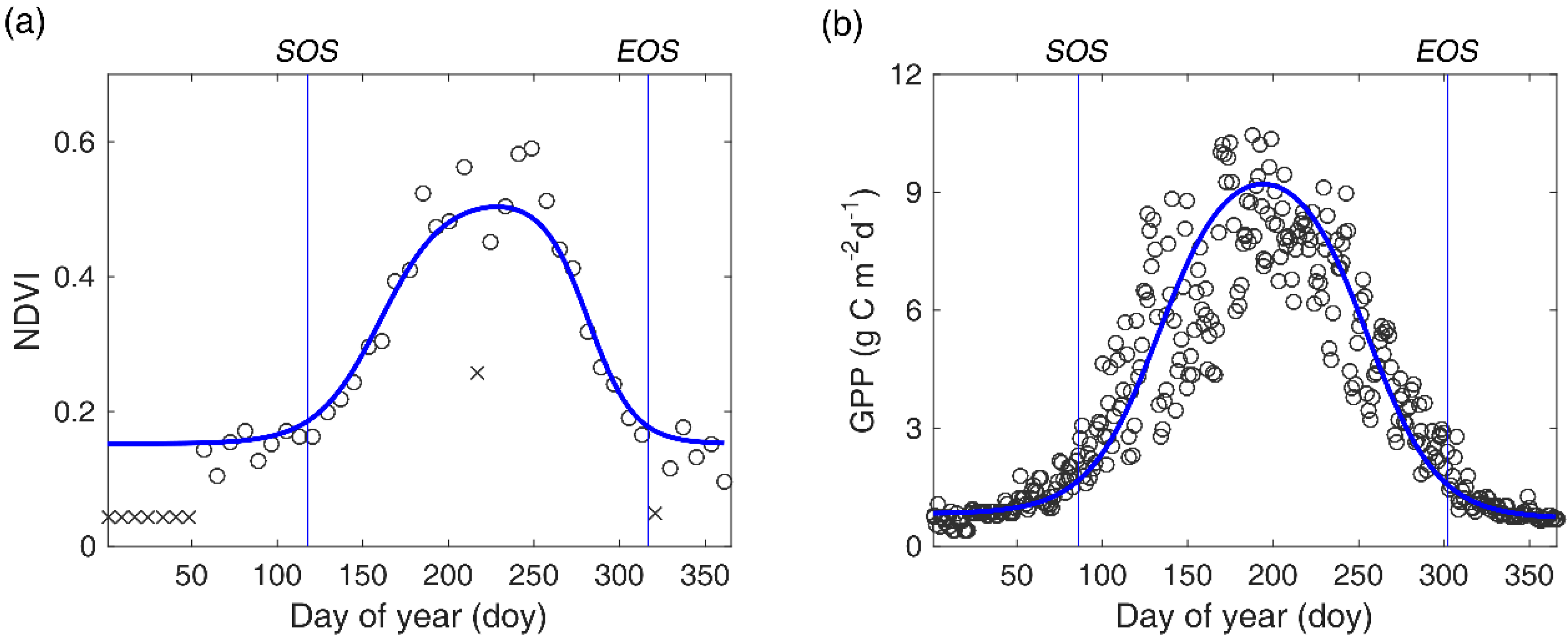
Figure 3.
Linear regression analysis between GPP-based SOS and MODIS-based SOS (a) and between GPP-based EOS and MODIS-based EOS (b).
Figure 3.
Linear regression analysis between GPP-based SOS and MODIS-based SOS (a) and between GPP-based EOS and MODIS-based EOS (b).

Figure 4.
Spatial pattern of multi-year average SOS (a) and multi-year average EOS (b). SOS (c) and EOS (d) comparison among meadow steppe, typical steppe, and desert steppe. Different letters (a–c, marked from the largest average to the smallest average) denote that there is a significant difference of SOS/EOS between the two grassland types at the level of 0.05.
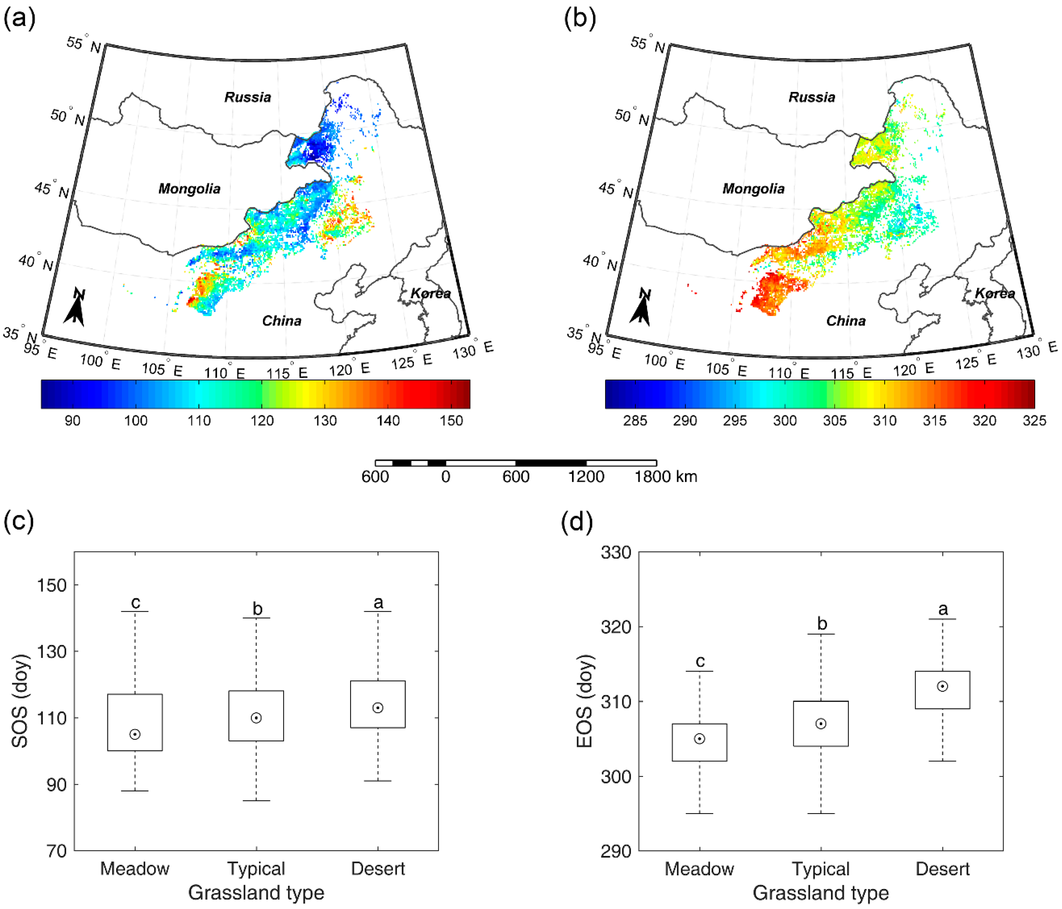
Figure 5.
Spatial patterns of correlation coefficients between: (a) SOS and pre-SOS temperature; (b) SOS and pre-SOS precipitation; (c) EOS and pre-EOS temperature; and (d) EOS and pre-EOS precipitation.
Figure 5.
Spatial patterns of correlation coefficients between: (a) SOS and pre-SOS temperature; (b) SOS and pre-SOS precipitation; (c) EOS and pre-EOS temperature; and (d) EOS and pre-EOS precipitation.

Figure 6.
Response rates of SOS to pre-SOS temperature (a) and precipitation (b), and response rates of EOS to pre-EOS temperature (c) and precipitation (d). The different letters indicate there is a significant difference of responding rates of SOS/EOS to temperature/precipitation between the two grassland types at the level of 0.05, while the same letter denotes there is no significant difference of responding rates of SOS/EOS to temperature/precipitation between the two grassland types.

Figure 7.
Spatial pattern of changing trends of SOS (a) and EOS (b). Frequency of changing trends of SOS (c) and EOS (d) in meadow steppe, typical steppe, and desert steppe. The vertical lines denote median values.
Figure 7.
Spatial pattern of changing trends of SOS (a) and EOS (b). Frequency of changing trends of SOS (c) and EOS (d) in meadow steppe, typical steppe, and desert steppe. The vertical lines denote median values.
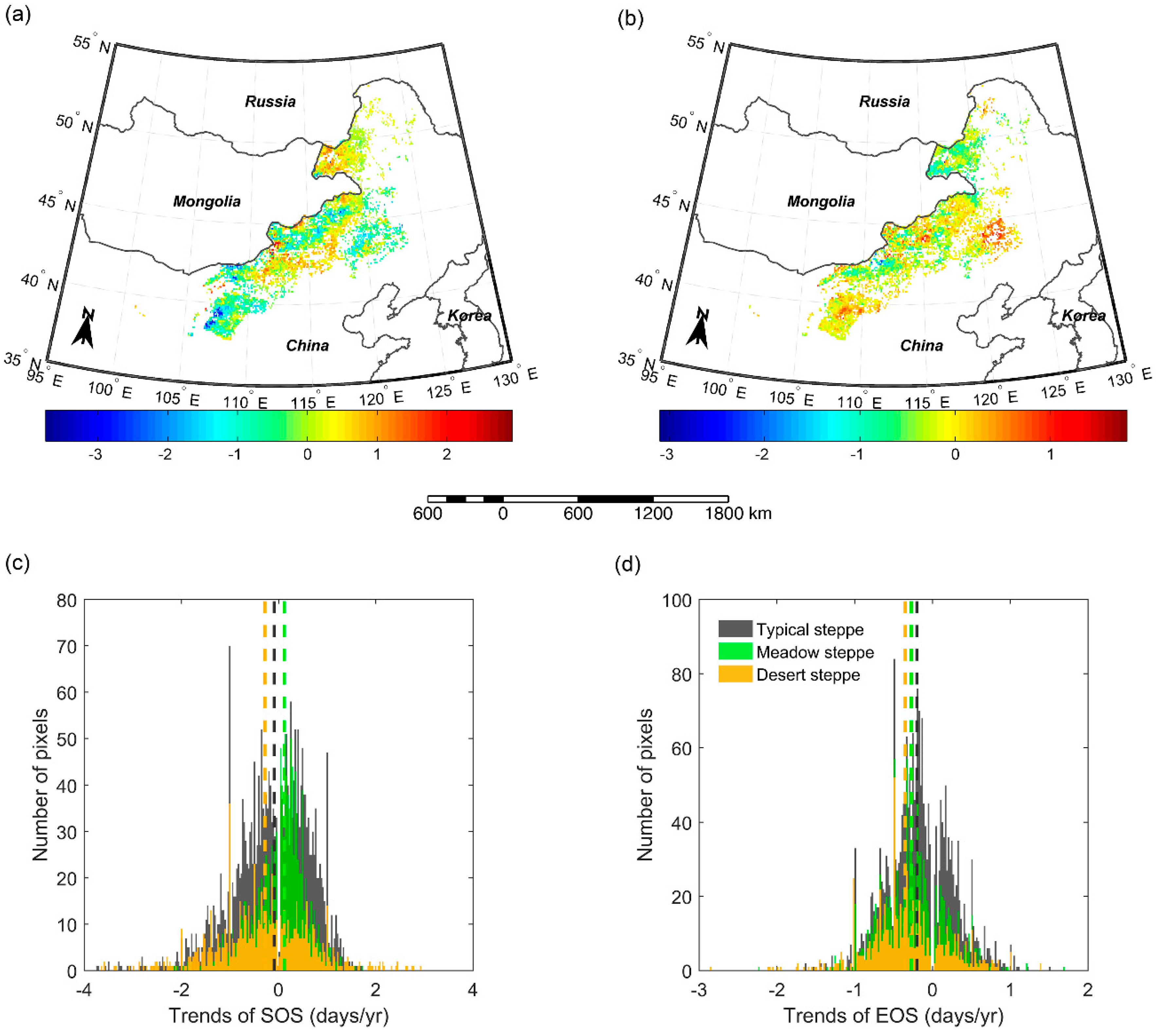
Figure 8.
Shifts of SOS (a) and EOS (b) from 2000–2004 to 2011–2015 in meadow steppe, typical steppe, and desert steppe. In the figure, the different letters denote there is a significant change of SOS/EOS from 2000–2004 to 2011–2015 at the level of 0.05, while the same letter denotes no significant change of SOS/EOS detected from 2000–2004 to 2011–2015.
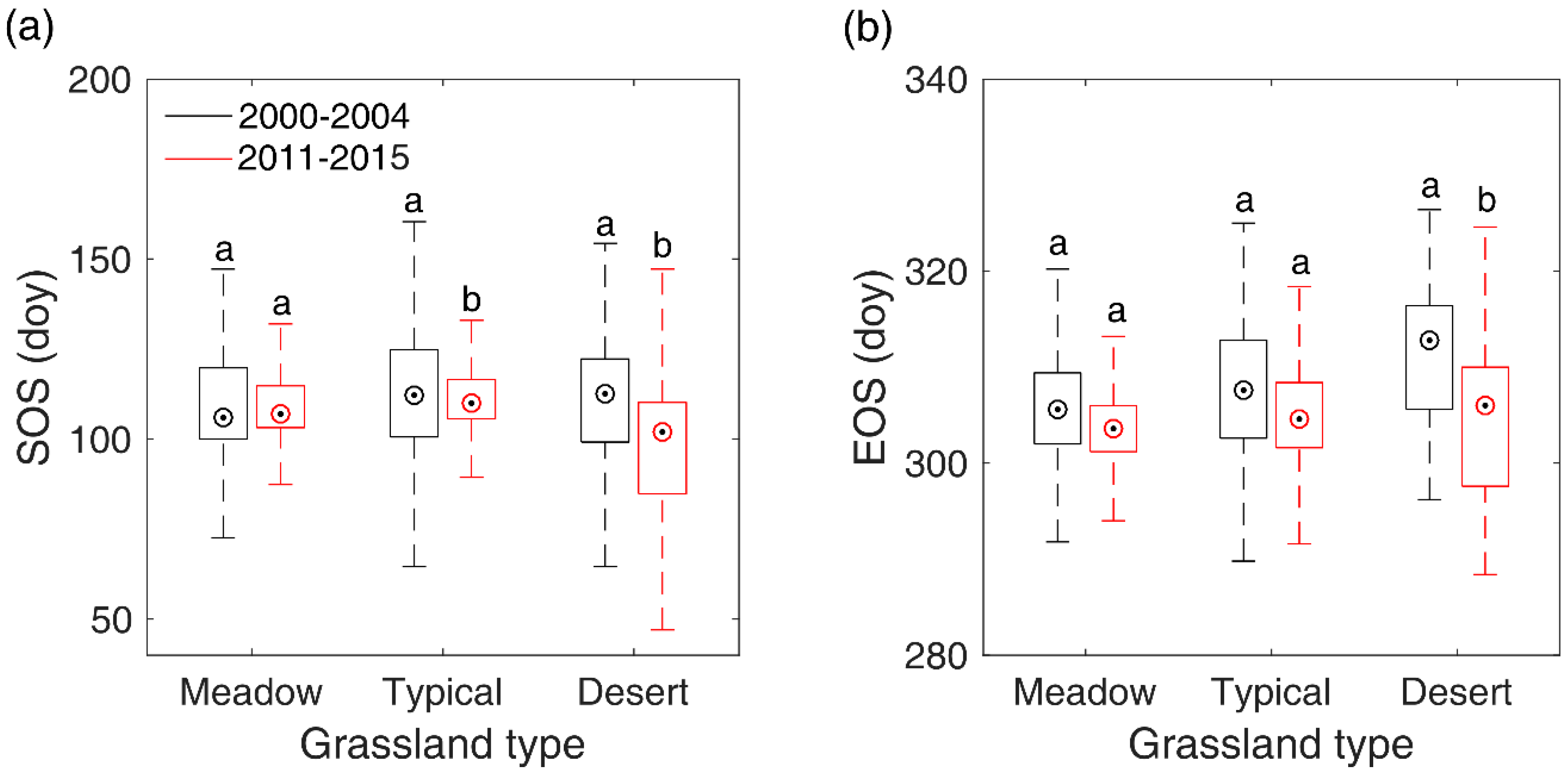
Figure 9.
Shifts of pre-SOS/EOS temperature (a) and precipitation (b) from 2000–2014 to 2011–2015 in typical steppe and desert steppe. In the figure, the different letters denote there is a significant change of temperature/precipitation from 2000–2014 to 2011–2015 at the level of 0.05, while the same letter denotes there is no significant variation of temperature/precipitation from 2000–2014 to 2011–2015.

Table 1.
Basic information of GPP observation sites, including geographical coordinate, observation time, vegetation type, and data source.
Table 1.
Basic information of GPP observation sites, including geographical coordinate, observation time, vegetation type, and data source.
| Site Name | Latitude (°N) | Longitude (°E) | Observation Time | Vegetation Type | Data Source |
|---|---|---|---|---|---|
| Duolun | 42.05 | 116.28 | 2008 | Typical steppe | FLUXNET2015 |
| Siwangziqi | 41.79 | 111.90 | 2012 | Desert steppe | FLUXNET2015 |
| Xilinhot_1 | 44.13 | 116.33 | 2004, 2006 | Typical steppe | Zhou et al., 2014 [57] |
| Xilinhot_2 | 43.55 | 116.67 | 2003, 2004 | Typical steppe | Hao, 2006 [58] |
Table 2.
Environmental conditions in meadow steppe, typical steppe, and desert steppe. ST: spring temperature; SP: spring precipitation; AT: autumn temperature; AP: autumn precipitation. Here, spring refers to March–May and autumn refers to September–November.
Table 2.
Environmental conditions in meadow steppe, typical steppe, and desert steppe. ST: spring temperature; SP: spring precipitation; AT: autumn temperature; AP: autumn precipitation. Here, spring refers to March–May and autumn refers to September–November.
| Type of Steppe | ST (°C) | SP (mm) | AT (°C) | AP (mm) |
|---|---|---|---|---|
| Meadow steppe | 5.1 | 55.9 | 4.9 | 72.0 |
| Typical steppe | 6.6 | 52.3 | 6.4 | 69.6 |
| Desert steppe | 7.1 | 36.0 | 6.8 | 53.7 |
© 2017 by the authors. Licensee MDPI, Basel, Switzerland. This article is an open access article distributed under the terms and conditions of the Creative Commons Attribution (CC BY) license (http://creativecommons.org/licenses/by/4.0/).
Share and Cite
MDPI and ACS Style
Ren, S.; Yi, S.; Peichl, M.; Wang, X. Diverse Responses of Vegetation Phenology to Climate Change in Different Grasslands in Inner Mongolia during 2000–2016. Remote Sens. 2018, 10, 17. https://doi.org/10.3390/rs10010017
AMA Style
Ren S, Yi S, Peichl M, Wang X. Diverse Responses of Vegetation Phenology to Climate Change in Different Grasslands in Inner Mongolia during 2000–2016. Remote Sensing. 2018; 10(1):17. https://doi.org/10.3390/rs10010017
Chicago/Turabian StyleRen, Shilong, Shuhua Yi, Matthias Peichl, and Xiaoyun Wang. 2018. "Diverse Responses of Vegetation Phenology to Climate Change in Different Grasslands in Inner Mongolia during 2000–2016" Remote Sensing 10, no. 1: 17. https://doi.org/10.3390/rs10010017
Note that from the first issue of 2016, this journal uses article numbers instead of page numbers. See further details here.