Sensitivity of BRDF, NDVI and Wind Speed to the Aerodynamic Roughness Length over Sparse Tamarix in the Downstream Heihe River Basin


1
Key Laboratory of Digital Earth Science, Institute of Remote Sensing and Digital Earth, Chinese Academy of Sciences, Beijing 100101, China
2
University of Chinese Academy of Sciences, Beijing 100049, China
*
Author to whom correspondence should be addressed.
Remote Sens. 2018, 10(1), 56; https://doi.org/10.3390/rs10010056
Submission received: 18 October 2017
/
Revised: 22 December 2017
/
Accepted: 28 December 2017
/
Published: 1 January 2018
Abstract
:The aerodynamic roughness length (z0m) is an important parameter that affects the momentum and energy exchange between the earth surface’s and the atmosphere. In this paper, the gradient wind speed data that were observed from May to October, 2014, at the Si Daoqiao station, which is located in an area of sparse Tamarix in the downstream region of the Heihe River Basin (HRB), are used to evaluate the sensitivity of the moderate-resolution imaging spectroradiometer (MODIS) near-infrared (NIR) bi-directional reflectance distribution function (BRDF) R, the MODIS/Landsat 8 normalized difference vegetation index (NDVI), and the wind speed at 5 m in comparison with the field-measured z0m. The results indicate that the NIR BRDF_R_MODIS and the NDVIMODIS/NDVILandsat8 are less sensitive indicators of the z0m over sparse Tamarix areas (R2: 0.0045 for NIR BRDF_RMODIS; R2: 0.0342 for NDVIMODIS; and, R2: 0.1646 for NDVILandsat8), which differs significantly from the results obtained by previous studies for farmlands and grasslands. However, there is a nearly linear correlation between the wind speed at 5 m and the z0m at the time scale of the NDVILandsat8 acquisitions (R2: 0.3696). Furthermore, the combination of the NDVI and wind speed at 5 m can significantly improve this correlation (R2: 0.7682 for NDVIMODIS; R2: 0.6304 for NDVILandsat8), whereas the combination of the NIR BRDF_RMODIS and wind speed at 5 m still has a low correlation (R2: 0.0886). Finally, the regional z0m of the oasis in the downstream region of the HRB was determined using Landsat 8 surface reflectance data and the wind speed data at the Si Daoqiao station, which properly reflect the temporal evolution of the z0m in that region. The parameterization scheme proposed in this paper has great potential to be applied to evapotranspiration, land surface, and hydrologic model simulations of sparse Tamarix at Si Daoqiao site in the future.

1. Introduction
The aerodynamic roughness length (z0m) is the height at which the wind speed approaches zero above the surface, and it plays a significant role in characterizing the interactions between the earth’s surface and the atmosphere, especially in terms of the momentum transport and energy exchange from bare soils to vegetation in sparsely vegetated regions [1,2,3]. An effective parameterized method for estimating the temporal and regional z0m is important to studies of evapotranspiration (ET), hydrology, and land surface processes in arid and semi-arid regions and promotes deeper understandings of water consumption and related hydrometeorological processes [4,5].
In the field, the z0m is traditionally calculated either using gradient wind data based on Monin-Obukhov similarity theory or from turbulence measurements from an eddy covariance instrument [6,7,8]. The regional AR has traditionally been given a long-term empirical value, according to a lookup table for different land cover types [9]. With the development of satellite remote sensing, time series of the normalized difference vegetation index (NDVI) or the leaf area index acquired from various optical satellites, including Landsat, Sentinel, and the moderate-resolution imaging spectroradiometer (MODIS), have mainly been used for z0m estimations of farmland and forests [10,11,12,13]. In recent years, multi-angle remote sensing information in the near-infrared (NIR) or shortwave infrared (SWIR) bands has been used to determine the z0m of farmlands over eight-day time intervals in the form of a bi-directional reflectance distribution function (BRDF) R index, which is the ratio of the weighting coefficient of the Li-sparse-reciprocal geometric scattering kernel and the weighting coefficient of the isotropic scattering contribution [14,15,16]. The combination of the NDVI and BRDF_R has been used to estimate the z0m of grassland and farmland areas [17,18]. However, whether the BRDF, NDVI, or their combinations are sensitive enough to estimate the z0m in sparsely vegetated regions remains unknown. If neither of these indicators can be used, it is urgent to determine what kind of new indicators should be used.
Therefore, this paper evaluates the sensitivity of BRDF_RMODIS, NDVIMODIS, NDVILandsat8, and wind speed in comparison with the field z0m to propose a new and effective parameterized scheme for estimating z0m under stations with sparse Tamarix, which represents an underlying surface of sparse vegetation. The field z0m data were calculated based on the gradient wind data measured at the Si Daoqiao station, which is located in the Ejin oasis, which is in the downstream region of the Heihe River Basin (HRB). The temporal NIR BRDF_RMODIS, NDVIMODIS, NDVILandsat8, and the average wind speed data at 5 m from May to October 2014 were collected and processed for this study. The proposed parameterized scheme that combines the NDVI and the wind speed at 5 m provides an effective solution to estimate z0m over sparse Tamarix at Si Daoqiao site and has significant application potential in the fields of ET, land surface, and hydrological model simulations. Finally, a regional map of z0m covering the oasis in the downstream region of the HRB is provided along with the temporal evolution.
2. Research Site and Experiments
The research site is located in the oasis of the Ejin Basin in the downstream area of the HRB covering 600 km2, which is a typical arid region with an annual mean precipitation of about 50 mm [19]. Due to the extremely arid nature of this region and its insufficient precipitation, the ecosystem is very fragile and is heavily dependent on the two branches of the Heihe River and Juyan Lake. The landscape is composed of sandy and gravelly deserts, a natural oasis dominated by Tamarix (30% cover), Populus euphratica (20%), and other arid-region species (10%), and lakes at the Heihe River terminus with overall flat topography [20,21,22]. The oasis in the Ejin Basin is essential to the arid landscape and is significant for the regional economy and ecosystem.
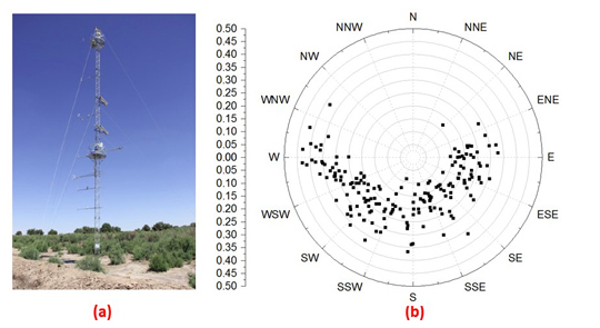
The superstation (101.12°E, 41.99°N, 935 m) is shown in Figure 1, and Tamarix is sparsely distributed around the base. The experimental site is used to collect multiplatform and multiscale observations of the land surface and hydrometeorological processes in this arid region. Intensive and long-term gradient meteorological observations of the wind, air temperature, and humidity at the study site were conducted at 6 levels (5 m, 7 m, 10 m, 15 m, 20 m, and 28 m) [23,24]. The manufacturer and model of each observational instrument are shown in Table 1.
3. Methodology
Several indices are introduced in Section 3.1, including BRDF_R, NDVI, the combined index of the wind speed at 5 m and the NDVI (WN), and the combined index of the wind speed at 5 m and the BRDF_R (WB). The field AR calculation method based on the gradient wind data is presented in Section 3.2.
3.1. Introduction to the Indices
3.1.1. NDVI
The NDVI was calculated based on the reflectance of the NIR and red bands, as follows:
where and are the reflectances from the NIR and red bands, respectively.
The MODIS MOD021km radiance data for 2014 were downloaded from the NASA MODIS Adaptive Processing System at a spatial resolution of 1 km [25,26] and then analysed to eliminate invalid data with apparent cloud coverage. The cloudless Landsat 8 surface reflectance data for 2014 were downloaded from the United States Geological Survey (USGS) EarthExplorer at a spatial resolution of 30 m [27,28]. Using these two datasets, the NDVI was calculated at spatial resolutions of 1 km and 30 m, respectively.
3.1.2. BRDF_R Index
MODIS predicts the bidirectional reflection characteristics of the earth’s surface using a BRDF model based on a linear combination of the RossThick and LiSparseR kernels. The simplified expression is as follows:
where and are the sun and viewing zenith angles, respectively; is the difference between the azimuth angles of the sun direction and the viewing direction; is the volume-scattering kernel based on the Ross-Thick function corrected for the hot-spot process; is the geometric kernel based on the Li-sparse-reciprocal function; is the weighting coefficient of the isotropic scattering contribution and is equal to the bidirectional reflectance for a view zenith angle of = 0 and a solar zenith angle of = 0; is the weighting coefficient of the Li-sparse-reciprocal geometric scattering kernel , which is derived from surface scattering and the geometric shadow casting theory; and, is the weighting coefficient for the Ross-Thick volume-scattering kernel , which is derived from radiative transfer models.
The BRDF_R index, which reflects the geometric roughness of the land surface, is calculated below:
The MODIS MCD43 B1 data from Collection 5 at eight-day intervals in 2014 were downloaded at a spatial resolution of 1 km from the Level-1 and Atmosphere Archive & Distribution System (LAADS) Distributed Active Archive Centre (DAAC), which is located at the Goddard Space Flight Centre in Greenbelt, Maryland [26,29]. These data were processed in batch mode, including format transformation, band extraction, projection transformation, subset formation, Julian day transformation, DN value type transformation, index calculation, and singular value elimination. The NIR BRDF_RMODIS data were used for this research based on the conclusions from [14].
3.1.3. Combined Index of Wind Speed and NDVI
The combined index of the wind speed and NDVI (WN) was calculated using the following formula:
where is calculated using Equation (1); and, WS is the average wind speed at 5 m on the date of the NDVI data.
3.1.4. Combined Index of Wind Speed and NIR BRDF_R
The combined index of the wind speed and NIR BRDF_R (WB) was calculated using the following formula:
where is the NIR BRDF_RMODIS index, which was calculated using Equation (2); and, WS is the average wind speed at 5 m for the time period of the BRDF_R data.
3.2. Field Aerodynamic Roughness Length Calculation
The original observed gradient data were pre-processed and quality controlled by removing singular and repeated values that exceeded the range of physical possibility via date format unification and data arrangement in a standard Excel format for ease of use. The original wind gradient data were collected at 10-min intervals, which resulted in 144 data records for each day.
The night AR values under stable conditions have been excluded in the averaging process as the weak relationship between the friction velocity at the ground surface, and the change velocity of wind speed with height, leads to an invalid result of the iteration calculation below. The effects of the underlying surface were minimized by selecting the wind and atmospheric profiles above the landscape for the field z0m calculations. The 10-min z0m values were acquired from the 10-min gradient data and then averaged into daily and concurrent average z0m values to be consistent with the various indicators used.
The meteorological gradient time series data from the wind gradient stations were processed to acquire the field z0m values based on the Monin-Obukhov similarity theory. Following Zhou et al., the wind velocities and air temperatures that were measured at different heights can be expressed as follows [30,31,32,33]:
where u is the wind velocity; is the friction velocity; k is the von Kármán constant (equal to 0.4); z is the height at which the wind velocity and air temperature are observed; is the air temperature of each layer, which is defined using the local surface pressure as the standard pressure; is the friction temperature; is the aerodynamic roughness length; d is the zero-plane displacement; is the thermal roughness length; is the skin temperature of the surface; and, L is the Obukhov length, which is calculated as follows [31]:
where g is the acceleration due to gravity (9.8 m/s2); T is the mean air temperature; P is the ambient air pressure; and, P0 is 101 kPa.
L is used to determine the atmospheric stability near the surface [34]. When Z/L = 0, there is neutral stratification. When Z/L < 0, there is unstable stratification. When Z/L > 0, there is stable stratification. and are the stability correction functions for the momentum and sensible heat transfers, respectively, which are determined based on the atmospheric stratification. These functions are expressed as follows, when Z/L < 0 [34]:
In the calculation, the least-square method is used. Equation (6) can be written as the following simplified form:
where , for Equation (6) and , and for Equation (7). Normally, d has a relationship with the vegetation height (h) that d equals to 0.67 h over surfaces covered by homogeneous vegetation [31,32], in consequence, d is calculated by iterative algorithm that increases from 0.1 m to 3 m at intervals of 0.1 m. For each given d, there is a correlation coefficient for the fitting Equation (17), and d is selected as the optimum value when the correlation coefficient reaches the maximum value. For given initial values of and , L is calculated using Equation (8) and , , and are determined using Equations (6) and (7). L is then calculated with Equation (8) using the values of and determined in last step until the difference between the values of L in two consecutive iterations was less than 0.01. After that, z0m can be calculated based on the linear fitting coefficients of Equation (6) based on the equation of .
4. Results and Analysis
Section 4.1 presents the example of the original observational data to demonstrate the consistency of the data at various layers and at different times. The trend analyses of the various indices are shown in Section 4.2, followed by the correlation relationship analyses in Section 4.3.
4.1. Consistency Analysis of the Observed Data
Examples of the original observed wind speed and air temperature data recorded at 10-min intervals on August 8, 2014, which is in the summer, are shown in Figure 2a,b, respectively, for heights of 5 m, 7 m, 10 m, 15 m, 20 m, and 28 m.
The temperature trends at different heights during the day (8:00–20:00) are nearly identical and follow the form of a parabolic curve. The maximum value of the maximum temperature occurs at 5 m, whereas the minimum value occurs at 20 m, and the maximum difference is only 0.49 °C. The differences between the temperatures at different heights are more significant at night (20:00–8:00). The higher the height is, the higher the temperature is. The overall changes in the air temperature at night remain consistent; they decrease to a minimum value, and then increase gradually. The maximum value of the minimum temperature occurs at 28 m, whereas the minimum value occurs at 5 m, and the maximum difference is 8.19 °C. The differences between the wind speeds at different heights is significant throughout the day and night, but the overall trends are consistent; the higher the height is, the stronger the wind is. The maximum value of the maximum wind speed occurs at 28 m, whereas the minimum value occurs at 5 m, and the maximum difference is 2.51 m/s. The maximum value of the minimum wind speed occurs at 28 m, whereas the minimum value occurs at 7 m, and the maximum difference is 1.38 m/s. In general, both the wind speed and air temperature display consistent variations over time in the different layers, which confirms the reliability of the original experimental instrument and data.
4.2. Trend Analyses of the Indicators
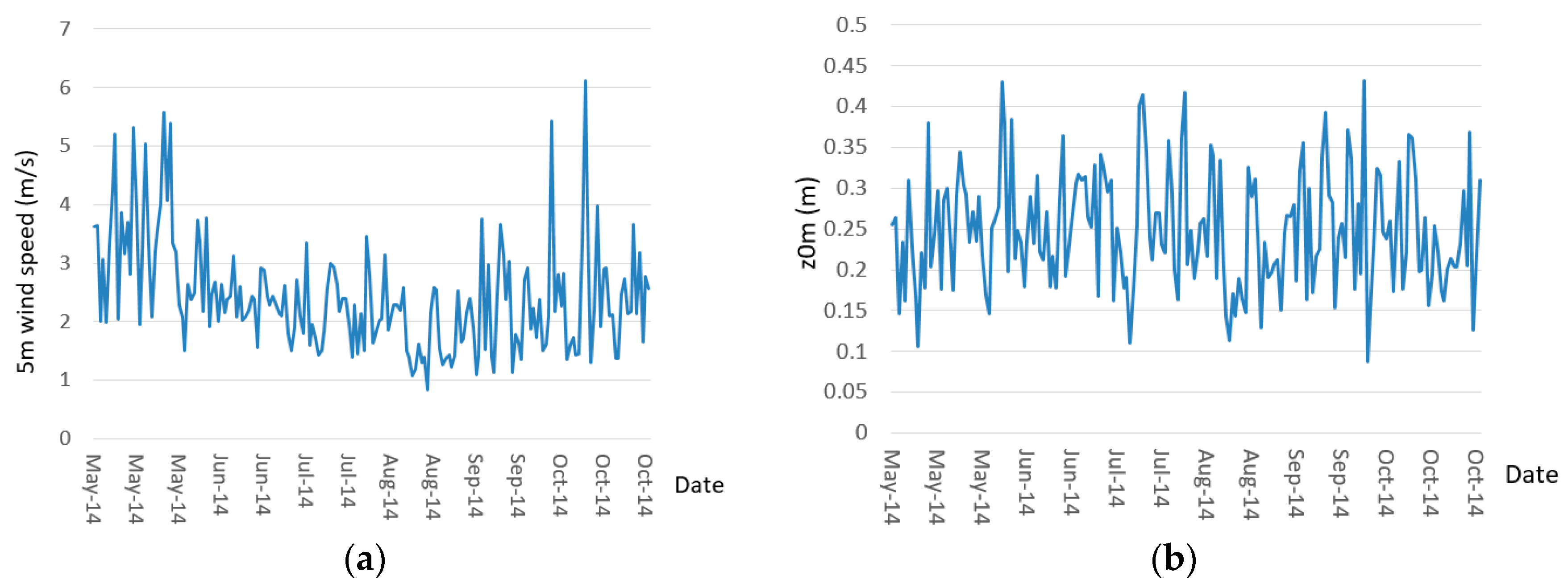
The cloud free remote sensing data at Si Daoqiao station for the monitoring period from May 1 to October 31, 2014, were acquired and are presented in Figure 3, including 22 NIR BRDF_RMODIS data (a), 30 NDVIMODIS data (b), and 16 NDVILandsat8 data (c). The daily average wind speed at 5 m and the field daily average z0m were obtained and are presented in Figure 4a,b.
The NIR BRDF_RMODIS data at Si Daoqiao station fluctuate in the range of 0.099–0.168 with an average of 0.135 and a standard deviation of 0.018, which reflect information about the spatial structure of the underlying surface (Figure 3a). The 1 km NDVIMODIS data are within the range of 0.113 to 0.347 with an average of 0.235 and a standard deviation of 0.077 (Figure 3b). The 30 m NDVI_Landsat8 data are in the range of 0.119 to 0.385 with an average of 0.272 and a standard deviation of 0.092 (Figure 3c). Although the NDVIMODIS and NDVILandsat8 values are not very high, they both show apparent vegetation growth curves between May and October due to the sparse Tamarix at Si Daoqiao site. The difference in the spatial scale of the NDVI values between the 1 km MODIS and 30 m Landsat 8 data is not significant in the study region.
The daily average wind speed at 5 m shows apparent fluctuations during the monitored period. These average wind speed was 3.41 m/s in May and then gradually decreased to 2.5 m/s, 2.169 m/s, and 1.8 m/s in June, July, and August, respectively, before increasing to 2.23 m/s in September and 2.43 m/s in October. The average wind speed during the entire period was 2.42 m/s, and the standard deviation was 0.95 m/s. The daily average z0m fluctuated significantly in the range of 0.087 m to 0.431 m with an average value of 0.247 m and a standard deviation of 0.072 m. The average z0m was 0.237 m in May, and it remained stable from June to July (0.267 m and 0.265 m, respectively). It then decreased to 0.219 m in August and then to 0.26 m in September, which is the same as in June and July. Finally, the average z0m decreased to 0.236 m in October.
4.3. Relationship Analyses
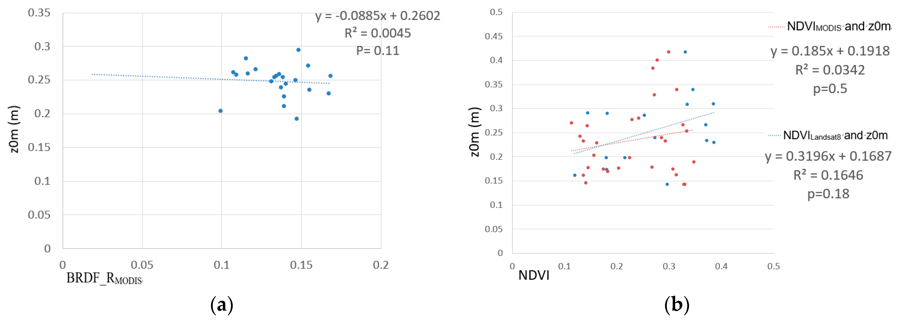
The relationships between the multiple indicators and the field z0m in the concurrent time periods from May to October are shown and analysed in this section with the p value of F-test. Specifically, the relationships between the remote sensing-based NIR BRDF_RMODIS, NDVIMODIS, NDVILandsat8 data, and the field z0m are shown in Figure 5a–c, respectively. The relationships between the wind speed at 5 m at different temporal scales and NIR BRDF_RMODIS, NDVIMODIS, NDVILandsat8, daily ground based observations and the field z0m are shown in Figure 6a–d, respectively. Furthermore, the relationships between the combination factors of WBMODIS, WNMODIS, WNlandsat8, and the field z0m are presented in Figure 7a–c, respectively.
The NIR BRDF_RMODIS data show almost no correlation with the field z0m with an R2 value of only 0.0045 and a small dispersion (Figure 5a). The NDVIMODIS data show very little correlation with the field z0m data with an R2 value of only 0.0342 and a large dispersion (Figure 5b). The NDVILandsat8 data also show little correlation with the field z0m with an R2 value of 0.1646 and a large dispersion (Figure 5c). These values clearly indicate that the NDVI and BRDF_R factors are not sensitive indicators for characterizing the z0m variations over sparse Tamarix at Si Daoqiao site, which is significantly different from previous studies of farmlands and grasslands [14,17,18]. The underlying surface at the Si Daoqiao station is composed of sparse Tamarix and bare soils (Figure 1). The sparse Tamarix plants are only 3 m high and have stable growth conditions, and the geometric surface structures of the bare soil are also consistent, which results in limited influences of the vegetation dynamics and the geometric surface structure on the z0m at Si Daoqiao site.
Because the temporal scales of the BRDF_RMODIS, NDVIMODIS, NDVILandsat8, and field wind speed data are different, the correlations between the wind speeds from these indicators and the concurrent field z0m values are as follows: R2 for BRDF_RMODIS: 0.1149; R2 for NDVIMODIS: 0.1659; R2 for NDVILandsat8: 0.3696; and, R2 for Daily wind speed: 0.2419. Positive linear correlations were observed for all four cases. The temporal scale has a large influence on the correlation between the wind speed and the field z0m. Although the R2 values are not high (maximum value of 0.3696), these results indicate that the wind speed at 5 m possibly has an influence on the z0m over sparse Tamarix at Si Daoqiao site. This finding is consistent with discussions in the literature that meteorological factors could influence the z0m [35,36].
The WNMODIS index has a significantly better correlation with the field z0m; it has a positive linear relationship with an R2 value of 0.7682 and a high aggregation degree, as shown in Figure 7b. As the WNMODIS value increases, the z0m value increases rapidly with a slope of 0.8141. The WN_Landsat8 also has a strong linear correlation with the field z0m with an R2 value of 0.6304 and a high aggregation degree, as shown in Figure 7c. However, WBMODIS has no correlation with the field z0m; the R2 value is only 0.0886, as shown in Figure 7a. This sharp contrast indicates that the combination of the wind speed and the NDVI in the form of an exponential function provides a suitably parameterized method to estimate the z0m and to characterize the interactions between sparse Tamarix and the atmosphere at Si Daoqiao site. This difference is mainly attributed to the relatively high wind speed in the downstream region of the arid HRB, the overall stable canopy structure, and growth profile, but with leaves falling process for the sparsely planted Tamarix in the region [20,21].
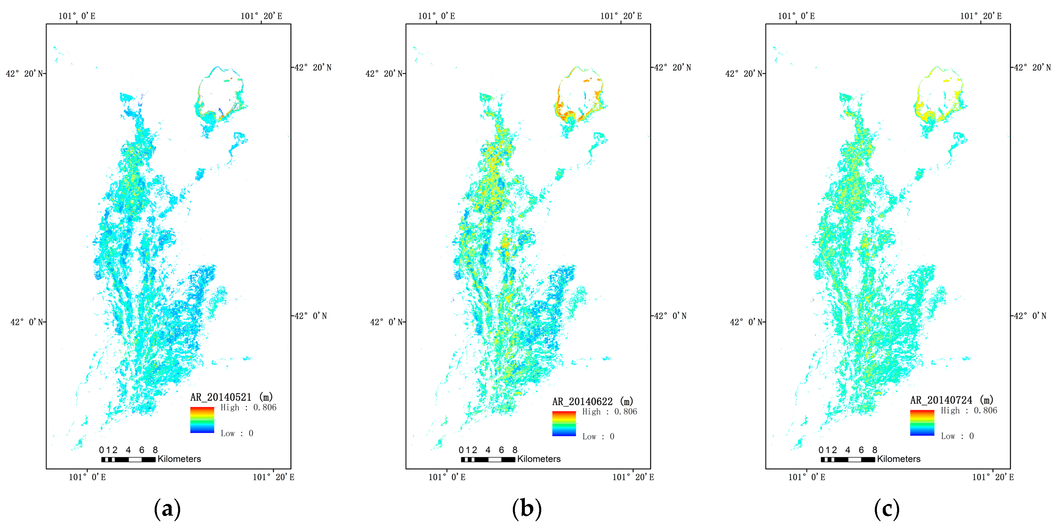
4.4. Regional z0m
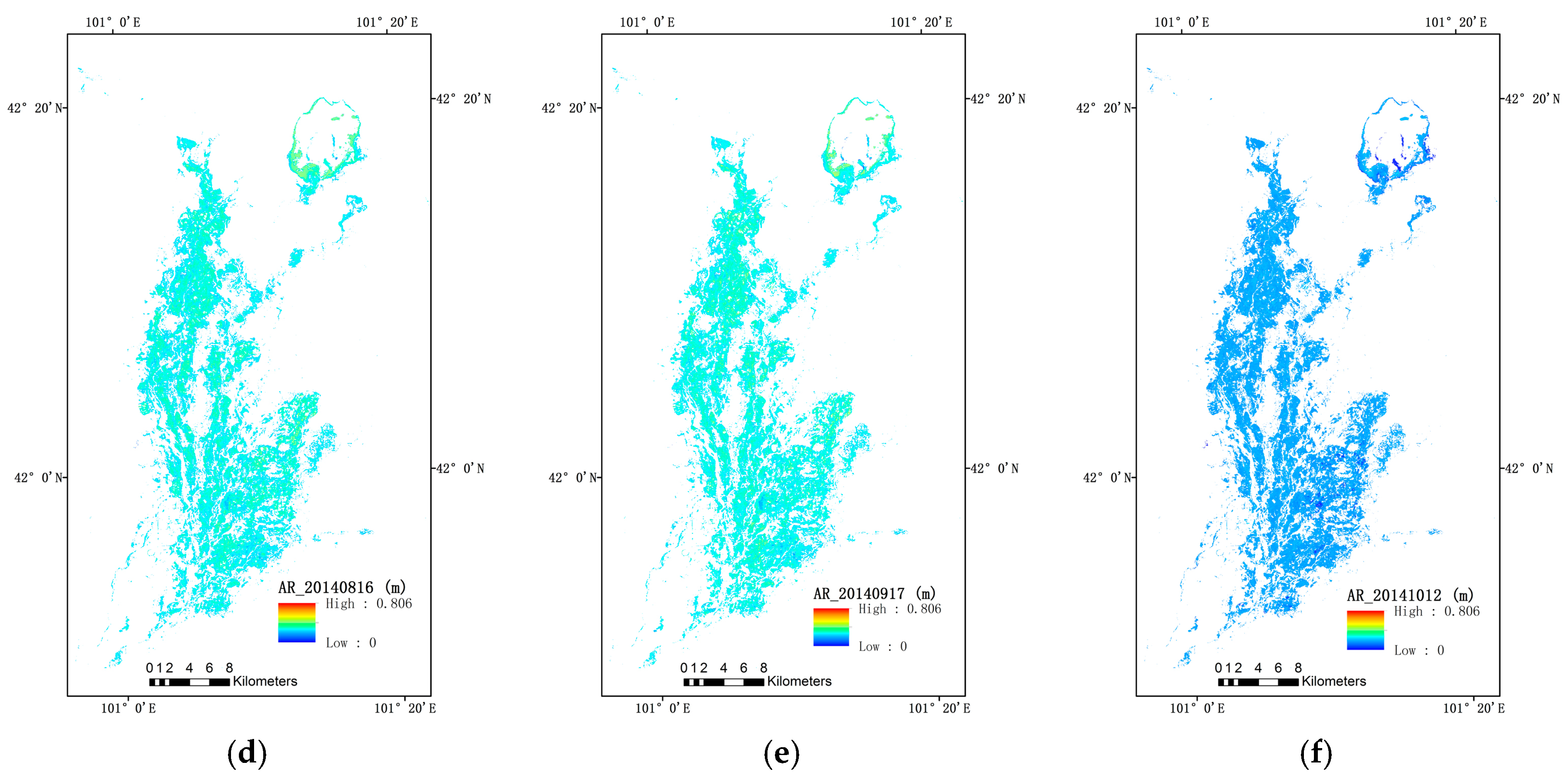
The regional z0m for the oasis in the downstream region of the HRB is derived based on the 30 m NDVILandsat8 data and the wind speed data from the Si Daoqiao station, as shown in Figure 8. The mask of the oasis is extracted from the Landsat 8-based NDVI on July 24, 2014, during which the Tamarix and Populus euphratica vegetation was in its peak growing phase. The standard deviation of each spatial result is only 0.07 m, 0.1 m, 0.07 m, 0.05 m, 0.04 m, and 0.02 m in sequence, indicating that the z0m value is in a stable range at Si Daoqiao site. Throughout the growing season, it reached a peak in July and then decreases beginning in August, when the leaves of Tamarix and Populus euphratica reach a plateau. The lowest spatial variability of all of the oasis pixels occurred in October, when nearly all of the vegetation leaves fell. The greatest spatial variability occurred in June, which indicates that the z0m had more significant spatial differentiation during this period. This is most likely attributable to the spatial differences in the growing conditions, the planting density, and water availability of the Tamarix, Populus euphratica and other arid-region species in this area.
5. Discussion
5.1. The Rationality of z0m
The average z0m value at the Si Daoqiao station was 0.247 m during the monitored period, whereas the height of the Tamarix at the Si Daoqiao station was approximately 2.35 m. The ratio between the field average z0m and the plant height is approximately 0.11. Langensiepen et al. (2009) calculated transpiration using the Penman–Monteith equation with a z0m of 0.13h [37]. Sánchez et al. (2009) fixed the z0m to 0.1h to estimate the energy fluxes [38]. A z0m experiment over arid South Tunisia during the spring of 2000 [36] found that the field average z0m is 0.353 m for sparse olive trees that are 3 m high with a spacing of 23 m. Thus, the z0m results in this study are comparable to published field results.
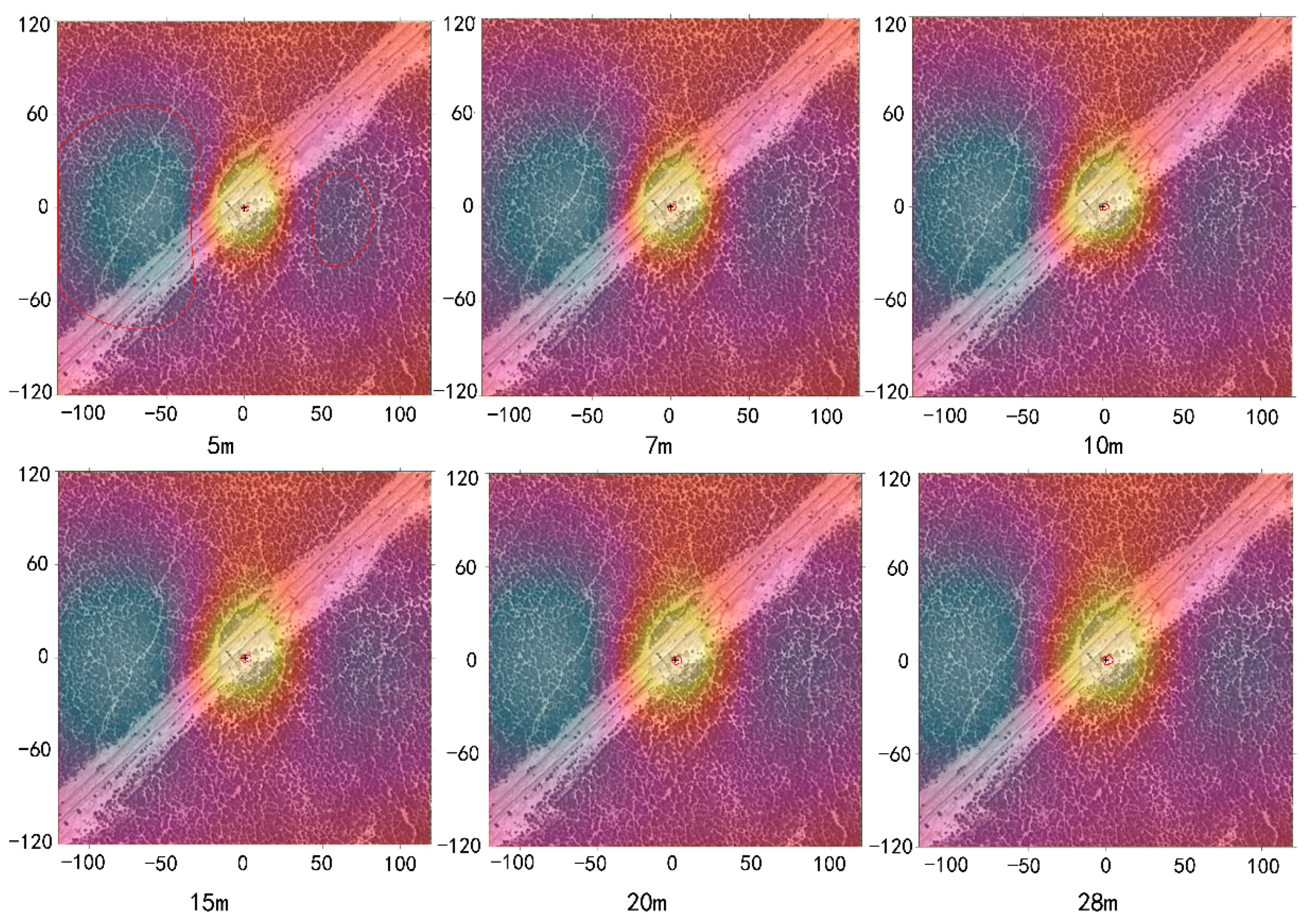
The gradient wind data at various layers were used to evaluate the footprint at Si Daoqiao station based on FFP footprint model [39], which is shown in Figure 9. The results shows that there is little difference for the footprint scale at different layers. Basically speaking, the underlying surface can be seen as homogeneous region across the footprint that is mainly covered by Tamarix and soil. Actually, the standard deviation of each spatial result is only 0.07 m, 0.1 m, 0.07 m, 0.05 m, 0.04 m, and 0.02 m in sequence, indicating the stable z0m value in this region.
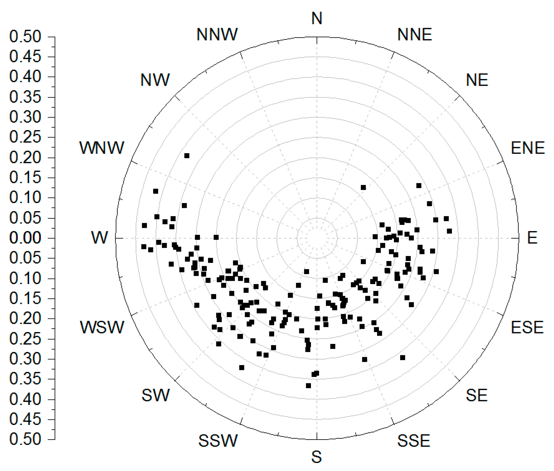
Figure 10 shows the rose chart between wind direction and AR at Si Daoqiao station, indicating that the main wind during the study time period is from north-western, northern, and north-eastern directions, which is consistent with the footprint estimation result. We will try to incorporate wind direction into our z0m estimation model further in the next step’s research.
5.2. The Relationship between Wind Speed and z0m at Si Daoqiao
The Tamarix is a shrub with the root underground as deep as 30 m. Therefore, it is very stable to hinder the wind and sands, which is different much from grass. The relationship between z0m and wind speed for Tamarix is more similar to that for forest. The documentations has reported that z0m usually increases with wind speed. For example, Schott (1980) found z0m to increase with growing wind speed values using 1975 data [40]. Vogt and Jaeger (1990) confirm these results further and reported that the relationship between z0m and wind speed is influenced by the lowest wind speed above the canopy and the heights of the wind profiles [41].
The relationship between z0m with wind speed is shown in Figure 11, indicating that z0m will increase with wind speed in phase І and Ш. When the wind speed increases to a certain extent and increases further, the billowing wave will form on the canopy surface, making the vegetation surface appear rougher, leading to the increase of the roughness length.
5.3. The Difference with Farmland and Grassland
A linear relationship with an R2 value of 0.8739 was identified between the field z0m and the NIR BRDF_RMODIS as derived from MODIS data for a maize-covered surface [14]. The BRDF_RMODIS and NDVIMODIS data are both sensitive indicators of the z0m over grasslands (R2: 0.5228 for NIR BRDF_RMODIS; R2: 0.579 for NDVIMODIS). The combined index has a significantly higher R2 value of 0.721, which is similar to the result inferred from the wind speed (R2: 0.7411) [17]. However, the result is different for the sparse Tamarix at Si Daoqiao site in this study. The NIR BRDF_RMODIS, NDVIMODIS, and NDVILandsat8 data are not sensitive indicators of z0m (R2: 0.0045 for NIR BRDF_RMODIS; R2: 0.0342 for NDVIMODIS; and, R2: 0.1646 for NDVILandsat8). The R2 value of the linear correlation between the wind speed at 5 m and the z0m at the time scale of the NDVILandsat8 acquisitions is 0.3696. The combination of the NDVI and wind speed at 5 m can significantly improve the correlation, with R2 values of 0.7682 for NDVIMODIS and 0.6304 for NDVILandsat8. These significant improvements of the correlation may be due to the typically arid features in the lower reaches of the HRB, which is composed of low Tamarix and bare soils with stable geometric structures at temporal scale. The sparse Tamarix plays a limited role in intercepting the winds, which are high at Si Daoqiao site. The combination of the NDVI, which characterizes the growth processes of vegetation leaves, and the wind speed can effectively represent the main influencing factors of the z0m of sparse Tamarix at Si Daoqiao site.
Although the inclusion of wind speed into z0m evaluations can significantly improve the correlations over sparse Tamarix at Si Daoqiao site, the wind speed near the surface can be difficult to acquire from current remote sensing measurements, which will restrict some spatial applications. Currently, the spatial interpolation of data from field meteorological stations may be used instead. The sensitivity of meteorological factors, such as wind speed, to the field z0m varies at different temporal scales, which is shown in Figure 6. In some cases, the correlation even disappears. Because the proposed model uses the wind speed as one of the input parameters, the temporal scale must be clarified. In this study, the acquisition date of the NDVIMODIS or NDVILandsat8 data is used as the reference date, during which the concurrent wind speed is calculated. In the next step of this work, we will test the robustness of the proposed parameterized method by determining the z0m over other sparsely vegetated stations to further validate its suitability and accuracy. Subsequent studies will also seek to identify other influencing factors to further improve the parameterization.
6. Conclusions
The main influencing factors of the z0m of sparse Tamarix at Si Daoqiao site are different from those of farmlands and grasslands. The BRDF_R and the NDVI are less sensitive indicators of the z0m in such areas between May and October (R2: 0.0045 for NIR BRDF_RMODIS; R2: 0.0342 for NDVIMODIS; and, R2: 0.1646 for NDVILandsat8). However, the combination of the wind speed at 5 m with the remote sensing-based NDVI can significantly improve the correlations with field z0m measurements during this growing period to R2 values of 0.7682 for NDVIMODIS and 0.6304 for NDVILandsat8, whereas the combination of the wind speed and NIR BRDF_RMODIS does not improve the correlation coefficient and results in an R2 value of only 0.0886. The proposed combination index based on the NDVI and the wind speed at 5 m in this study provides a new parameterization scenario for estimating z0m values in areas of Tamarix from May to October and has significant potential to be applied to ET, hydrology, and land surface model simulations at Si Daoqiao site.
Acknowledgments
This work was supported by Key Research Program of Frontier Sciences, CAS, Grant No. QYZDY-SSW-DQC014 and by National Natural Science Foundation of China (NSFC, Grant No. 91025007 and No. 41501479). The authors express their gratitude to the HiWATER-MUSOEXE project and the Cold and Arid Regions Science Data Centre in Lanzhou (http://westdc.westgis.ac.cn) for providing data from the Si Daoqiao station. Many thanks are extended to Yanlian Zhou of Nanjing University for providing assistance with the field AR calculation programme. The MCD43B-MODIS/Terra + Aqua BRDF/Albedo Model Parameters 16-Day L3 Global 1 km SIN Grid datasets and the MODIS 1B Calibrated Radiances Product were acquired from the Level-1 and Atmosphere Archive & Distribution System (LAADS) Distributed Active Archive Centre (DAAC), which is located at the Goddard Space Flight Centre in Greenbelt, Maryland (https://ladsweb.modaps. eosdis.nasa.gov/). The Landsat 8 surface reflectance data for 2014 were downloaded from the United States Geological Survey (USGS) EarthExplorer (https://earthexplorer.usgs.gov/).
Author Contributions
Qiang Xing and Bingfang Wu designed and conducted the experiment, Mingzhao Yu, Nana Yan and Weiwei Zhu provided suggestions for the analysis, Qiang Xing wrote the manuscript, and Bingfang Wu revised the manuscript.
Conflicts of Interest
The authors declare that they have no conflicts of interest.
References
- Blumberg, D.G.; Greeley, R. Field studies of aerodynamic roughness length. J. Arid Environ. 1993, 25, 39–48. [Google Scholar] [CrossRef]
- Monteith, J. Principles of Environmental Physics; Edward Arnold: London, UK, 1973. [Google Scholar]
- Stull, R.B. An Introduction to Boundary Layer Meteorology; Springer: New York, NY, USA, 1988. [Google Scholar]
- Nichols, W.D. Energy budgets and resistances to energy transport in sparsely vegetated rangeland. Agric. For. Meteorol. 1992, 60, 221–247. [Google Scholar] [CrossRef]
- Mackinnon, D.J.; Clow, G.D.; Tigges, R.K.; Reynolds, R.L.; Chavez, P.S., Jr. Comparison of aerodynamically and model-derived roughness lengths (Z0) over diverse surfaces, central Mojave Desert, California, USA. Geomorphology 2004, 63, 103–113. [Google Scholar] [CrossRef]
- Driese, K.L.; Reiners, W.A. Aerodynamic roughness parameters for semi-arid natural shrub communities of Wyoming, USA. Agric. For. Meteorol. 1997, 88, 1–14. [Google Scholar] [CrossRef]
- Marticorena, B.; Kardous, M.; Bergametti, G.; Callot, Y.; Chazette, P.; Khatteli, H.; Hegarat-Mascle, S.L.; Maille, M.; Rajot, J.L.; Vidal-Madjar, D.; et al. Surface and aerodynamic roughness in arid and semiarid areas and their relation to radar backscatter coefficient. J. Geophys. Res. 2006, 111, F03017. [Google Scholar] [CrossRef]
- Martano, P. Estimation of surface roughness length and displacement height from single-level sonic anemometer data. J. Appl. Meteorol. 2000, 39, 708–715. [Google Scholar] [CrossRef]
- Allen, R.G.; Tasumi, M.; Morse, A.; Trezza, R.; Wright, J.L.; Bastiaanssen, W.; Kramber, W.; Lorite, I.; Robison, C.W. Satellite-based energy balance for mapping evapotranspiration with internalized calibration (METRIC)—Model. J. Irrig. Drain. Eng. 2007, 133, 395–406. [Google Scholar] [CrossRef]
- Bastiaanssen, W.G.M.; Menenti, M.; Feddes, R.A.; Holtslag, A.A.M. A remote sensing surface energy balance algorithm for land (SEBAL)—1. Formulation. J. Hydrol. 1998, 212–213, 198–212. [Google Scholar] [CrossRef]
- Jaeil, C.; Shin, M.; Pat, J.F.Y.; Wonsik, K.; Shinjiro, K.; Taikan, O. Testing the hypothesis on the relationship between aerodynamic roughness length and albedo using vegetation structure parameters. Int. J. Biometeorol. 2012, 56, 411–418. [Google Scholar] [CrossRef]
- Jordan, S.B.; Michael, F.J.; Richard, D.C. Time series vegetation aerodynamic roughness fields estimated from modis observations. Agric. For. Meteorol. 2005, 135, 252–268. [Google Scholar] [CrossRef]
- Schaudt, K.J.; Dikinson, R.E. An approach to deriving roughness length and zero-plane displacement height from satellite data, prototyped with BOREAS data. Agric. For. Meteorol. 2000, 104, 143–155. [Google Scholar] [CrossRef]
- Wu, B.F.; Xing, Q.; Yan, N.N.; Zhu, W.W.; Zhuang, Q.F. A linear relationship between temporal multiband MODIS BRDF and aerodynamic roughness in HiWATER wind gradient data. IEEE Geosci. Remote Sens. Lett. 2015, 12, 507–511. [Google Scholar] [CrossRef]
- Vermote, E.; Justice, C.O.; Bréon, F.M. Towards a generalized approach for correction of the BRDF effect in MODIS directional reflectance. IEEE Trans. Geosci. Remote Sens. 2009, 47, 898–908. [Google Scholar] [CrossRef]
- Roujean, J.L.; Leroy, M.; Deschamps, P.Y. A bidirectional model of the Earth’s surface for the correction of remote sensing data. J. Geophys. Res. 1992, 97, 20455–20468. [Google Scholar] [CrossRef]
- Xing, Q.; Wu, B.F.; Yan, N.N.; Yu, M.Z.; Zhu, W.W. Evaluating the relationship between field aerodynamic roughness and the MODIS BRDF, NDVI, and wind speed over grassland. Atmosphere 2017, 8, 16. [Google Scholar] [CrossRef]
- Yu, M.Z.; Wu, B.F.; Yan, N.N.; Xing, Q.; Zhu, W.W. A method for estimating the aerodynamic roughness length with NDVI and BRDF signatures using multi-temporal Proba-V data. Remote Sens. 2017, 9, 6. [Google Scholar] [CrossRef]
- Li, X.; Cheng, G.D.; Liu, S.M.; Xiao, Q.; Ma, M.G.; Jin, R.; Che, T.; Liu, Q.H.; Wang, W.Z.; Qi, Y.; et al. Heihe Watershed Allied Telemetry Experimental Research (HiWATER): Scientific objectives and experimental design. Bull. Am. Meteorol. Soc. 2013, 94, 1145–1160. [Google Scholar] [CrossRef]
- Li, X.; Liu, S.M.; Liu, Q.H.; Ma, M.G.; Xiao, Q.; Jin, R.; Che, T.; Wang, W.Z.; Qi, Y.; Guo, J.W.; et al. Implementation Plan of the Heihe Watershed Allied Telemetry Experimental Research (HiWATER); Cold and Arid Regions Environmental and Engineering Research Institute, Chinese Academy of Sciences: Lanzhou, China, 2012. [Google Scholar]
- Li, Z.S.; Jia, L.; Hu, G.C.; Lu, J.; Zhang, J.X.; Chen, Q.T.; Wang, K. Estimation of growing season daily ET in the middle stream and downstream areas of the Heihe River Basin using HJ-1 data. IEEE Geosci. Remote Sens. 2015, 12, 948–952. [Google Scholar] [CrossRef]
- Zhu, W.W.; Wu, B.F.; Yan, N.N.; Feng, X.; Xing, Q. A method to estimate diurnal surface soil heat flux from MODIS data for a sparse vegetation and bare soil. J. Hydrol. 2014, 511, 139–150. [Google Scholar] [CrossRef]
- Liu, S.M.; Xu, Z.W.; Zhu, Z.L.; Jia, Z.Z.; Zhu, M.J. Measurements of evapotranspiration from eddy-covariance systems and large aperture scintillometers in the Hai River Basin, China. J. Hydrol. 2013, 487, 24–38. [Google Scholar] [CrossRef]
- Liu, S.M.; Xu, Z.W.; Wang, W.Z.; Bai, J.; Jia, Z.; Zhu, M.; Wang, J.M. A comparison of eddy-covariance and large aperture scintillometer measurements with respect to the energy balance closure problem. Hydrol. Earth Syst. Sci. 2011, 15, 1291–1306. [Google Scholar] [CrossRef]
- MODIS Characterization Support Team. MODIS 1km Calibrated Radiances Product; NASA MODIS Adaptive Processing System, Goddard Space Flight Centre: Greenbelt, MD, USA, 2015.
- LAADS DAAC. Available online: https://ladsweb.modaps.eosdis.nasa.gov/ (accessed on 20 May 2017).
- Vermote, E.; Justice, C.; Claverie, M.; Franch, B. Preliminary analysis of the performance of the Landsat 8/OLI land surface reflectance product. Remote Sens. Environ. 2016, 185, 46–56. [Google Scholar] [CrossRef]
- EarthExplorer. Available online: https://earthexplorer.usgs.gov/ (accessed on 10 July 2017).
- Schaaf, C.; Liu, J.C.; Gao, F.; Jiao, Z.T.; Shuai, Y.M.; Strahler, A. MCD43B1—MODIS/Terra+Aqua BRDF/Albedo Model Parameters 16-Day L3 Global 1km SIN Grid, C5, NASA Level-1 and Atmosphere Archive & Distribution System (LAADS) Distributed Active Archive Centre (DAAC); Goddard Space Flight Centre: Greenbelt, MD, USA, 2015.
- Panofsky, H.A. Determination of stress from wind and temperature measurements. Q. J. R. Meteorol. Soc. 1963, 89, 85–94. [Google Scholar] [CrossRef]
- Zhou, Y.L.; Ju, W.M.; Sun, X.M.; Wen, X.F. Significant decrease of uncertainties in sensible heat flux simulation using temporally variable aerodynamic roughness in two typical forest ecosystems of China. J. Appl. Meteorol. Climatol. 2012, 51, 1099–1110. [Google Scholar] [CrossRef]
- Raupach, M.R. Drag and drag partition on rough surfaces. Bound.-Layer Meteorol. 1992, 60, 375–395. [Google Scholar] [CrossRef]
- Raupach, M.R. Simplified expressions for vegetation roughness length and zero-plane displacement as functions of canopy height and area index. Bound.-Layer Meteorol. 1994, 71, 211–216. [Google Scholar] [CrossRef]
- Zhou, Y.L.; Sun, X.M.; Zhu, Z.L.; Zhang, R.H.; Tian, J.; Liu, Y.F.; Guan, D.X.; Yuan, G.F. Surface roughness length dynamic over several different surfaces and its effects on modelling fluxes. Sci. China Ser. D 2006, 49, 262–272. [Google Scholar] [CrossRef]
- Faivre, R.; Colin, J.; Menenti, M. Evaluation of Methods for aerodynamic roughness length retrieval from very high-resolution imaging LIDAR observations over the Heihe Basin in China. Remote Sens. 2017, 9, 63. [Google Scholar] [CrossRef]
- Zhang, Q.; Zeng, J.; Yao, T. Interaction of aerodynamic roughness length and wind flow conditions and its parameterization over vegetation surface. Chin. Sci. Bull. 2012, 57, 1559–1567. [Google Scholar] [CrossRef]
- Langensiepen, M. Quantifying the uncertainties of transpiration calculations with the Penman—Monteith equation under different climate and optimum water supply conditions. Agric. For. Meteorol. 2009, 149, 1063–1072. [Google Scholar] [CrossRef]
- Sáncheza, J.M.; Caselles, V.; Niclòs, R.; Coll, C.; Kustas, W.P. Estimating energy balance fluxes above a boreal forest from radiometric temperature observations. Agric. For. Meteorol. 2009, 149, 1037–1049. [Google Scholar] [CrossRef]
- Kljun, N.; Calanca, P.; Rotach, M.W.; Schmid, H.P. A simple two-dimensional parameterization for Flux Footprint Prediction (FFP). Geosci. Model Dev. 2015, 8, 3695–3713. [Google Scholar] [CrossRef]
- Schott, R. Investigations on the Energy Balance Components in the Atmospheric Boundary Layer on the Example of a Pine Stock in the Upper Rhine Plain (Hartheim/Rhein); German Weather Service: Frankfurter, Germany, 1980. [Google Scholar]
- Vogt, R.; Jaeger, L. Evaporation from a pine forest. Using the aerodynamic and Bowen ratio method. Agric. For. Meteorol. 1990, 50, 39–54. [Google Scholar] [CrossRef]
Figure 1.
(a) Landscape of the Heihe River Basin (HRB), (b) landscape of the Si Daoqiao site, and (c) observational equipment [19].
Figure 1.
(a) Landscape of the Heihe River Basin (HRB), (b) landscape of the Si Daoqiao site, and (c) observational equipment [19].
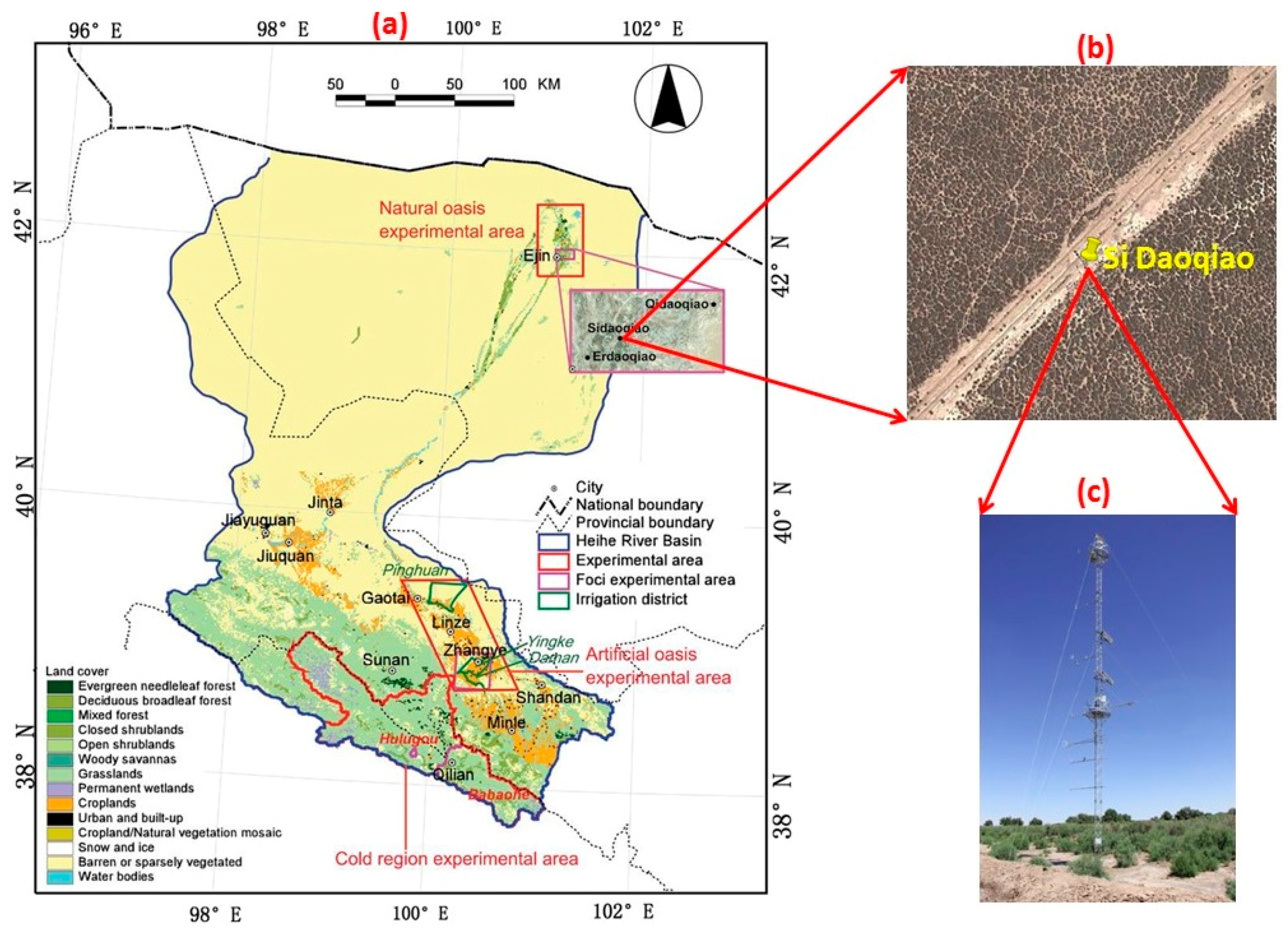
Figure 2.
Original observed air temperature (a) and wind speed (b) data at heights of 5 m, 7 m, 10 m, 15 m, 20 m, and 28 m on 8 August 2014.
Figure 2.
Original observed air temperature (a) and wind speed (b) data at heights of 5 m, 7 m, 10 m, 15 m, 20 m, and 28 m on 8 August 2014.
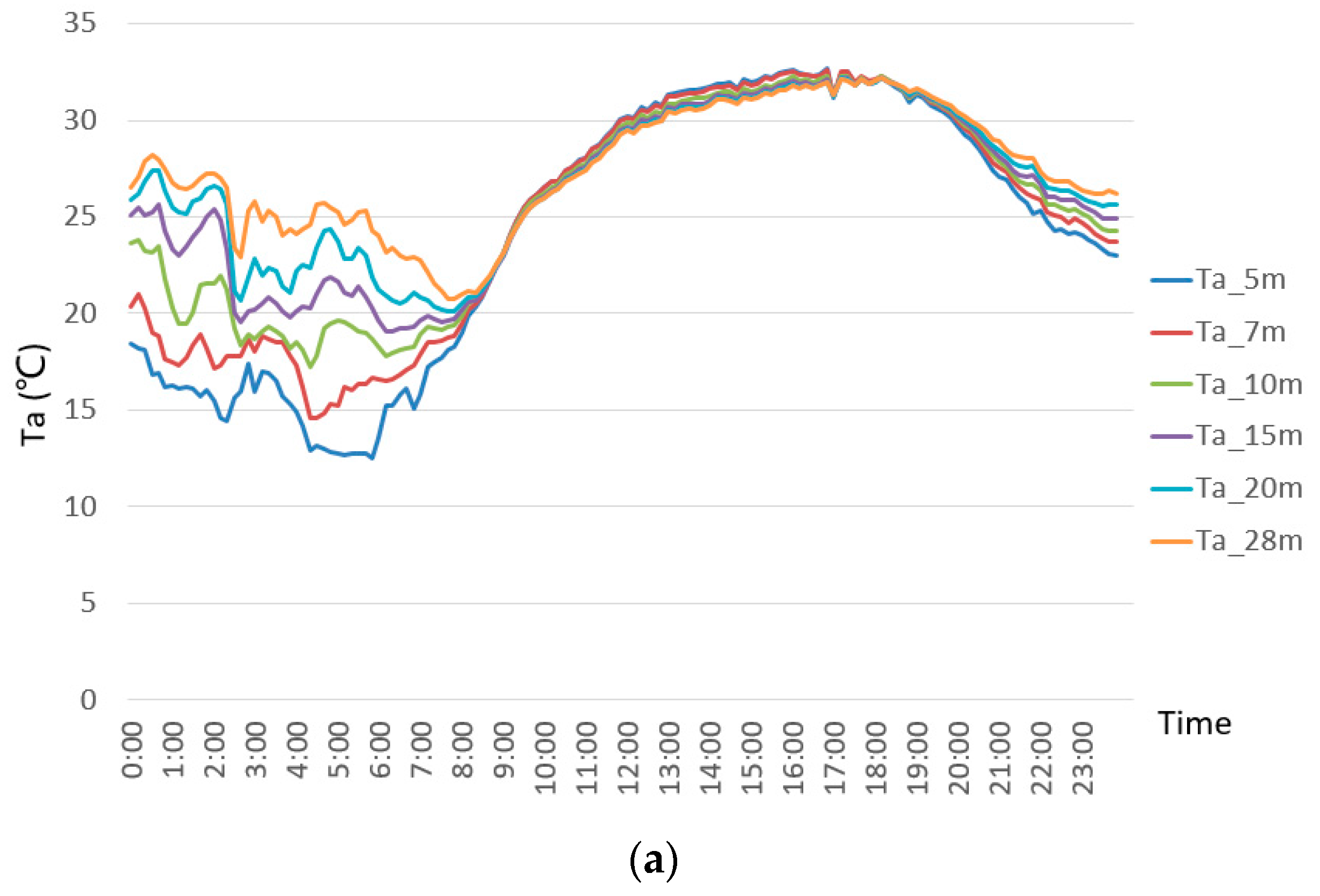
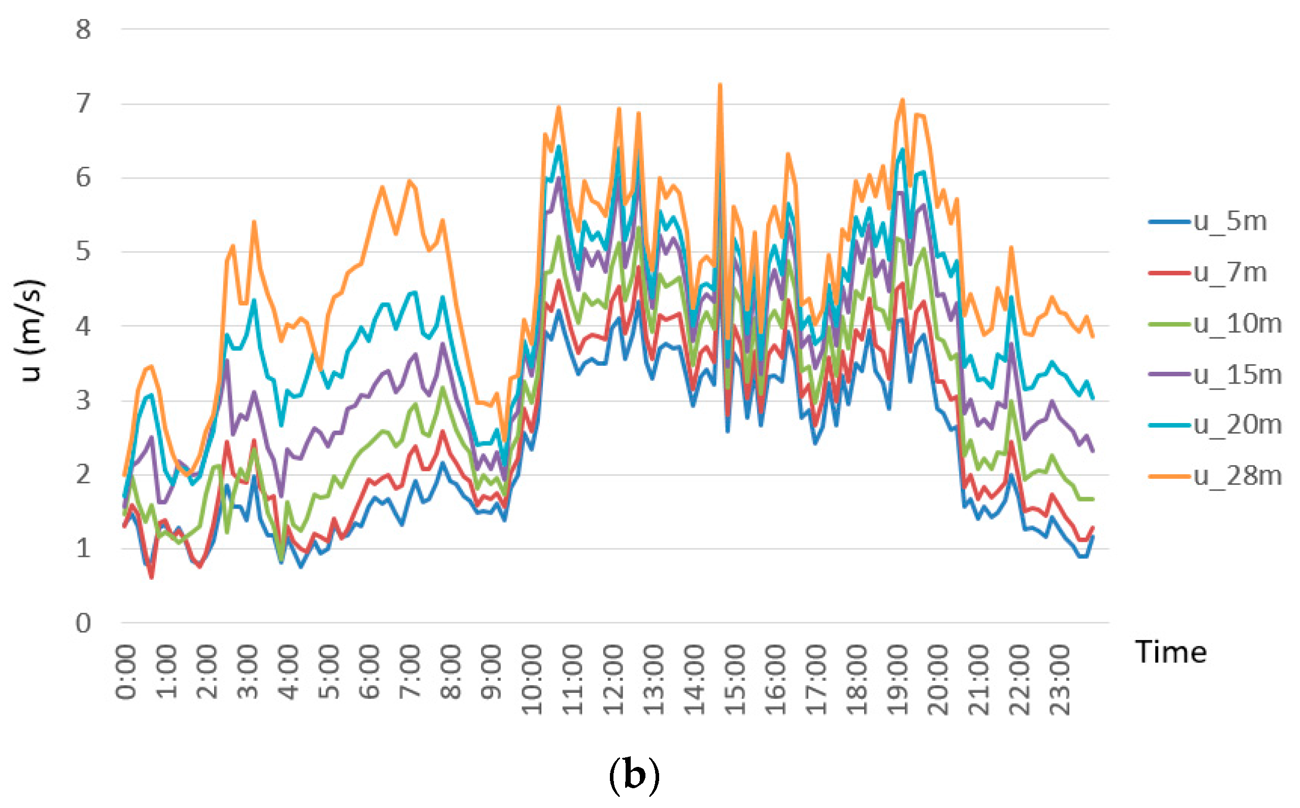
Figure 3.
Variations of NDVIMODIS, NDVILandsat8 and BRDFMODIS from May to October, 2014.
Figure 4.
Variations of the 5 m wind speed (a) and the field z0m (b) from May to October, 2014.

Figure 5.
Relationships between NIR BRDF_RMODIS and the field z0m (a) and between NDVIMODIS and the field z0m and between NDVILandsat8 and the field z0m (b) at the Si Daoqiao station from May to October, 2014.
Figure 5.
Relationships between NIR BRDF_RMODIS and the field z0m (a) and between NDVIMODIS and the field z0m and between NDVILandsat8 and the field z0m (b) at the Si Daoqiao station from May to October, 2014.

Figure 6.
Relationships between wind speed on BRDF_RMODIS days and the field z0m (a), between wind speed on NDVIMODIS days and the field z0m (b), between wind speed on NDVILandsat8 days and the field z0m (c), and between Daily wind speed and the field z0m (d) at the Si Daoqiao station from May to October in 2014.
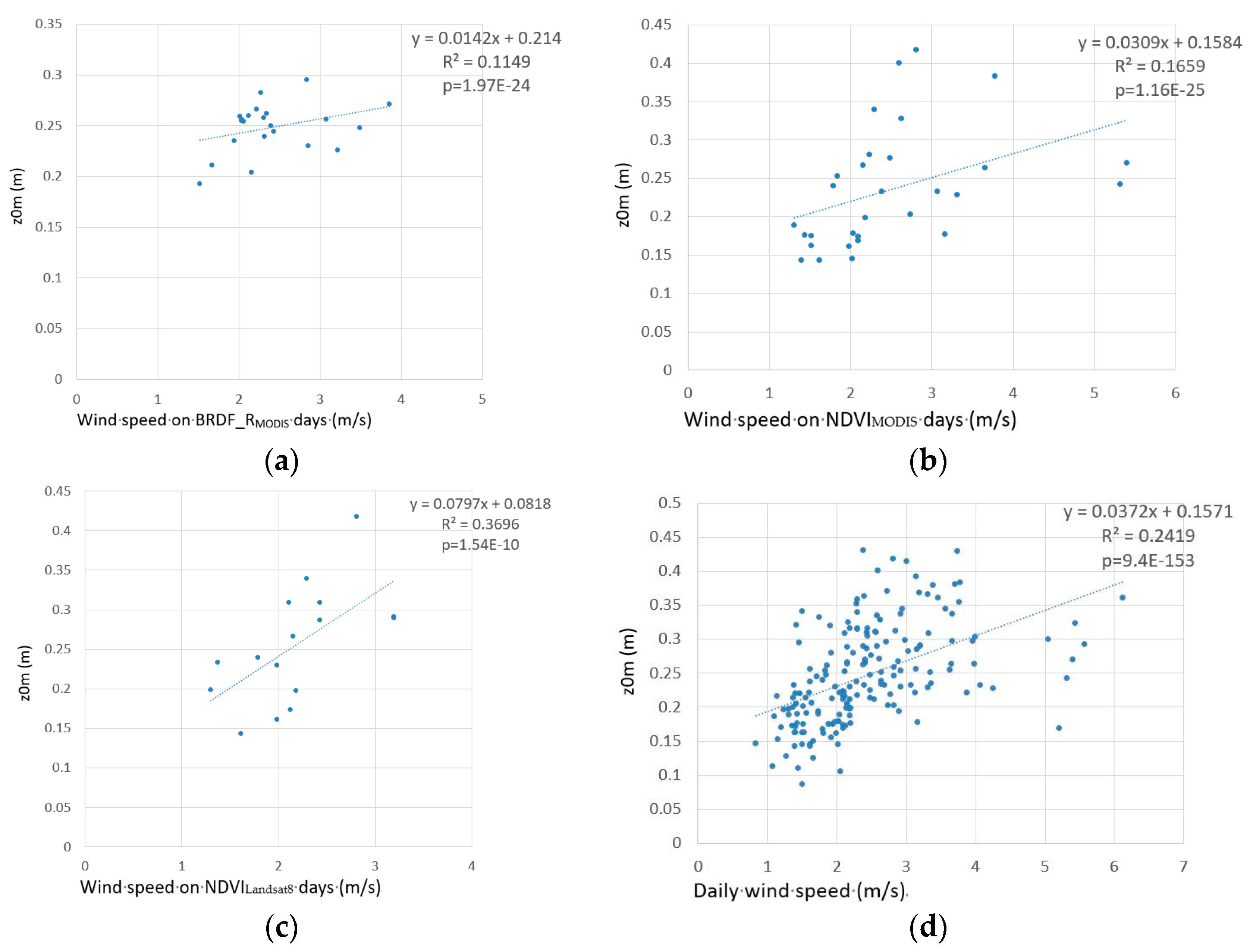
Figure 7.
Relationships between WBMODIS and the field z0m (a), between WNMODIS and the field z0m (b), and between WNLandsat8 and the field z0m (c) at the Si Daoqiao station from May to October in 2014.
Figure 7.
Relationships between WBMODIS and the field z0m (a), between WNMODIS and the field z0m (b), and between WNLandsat8 and the field z0m (c) at the Si Daoqiao station from May to October in 2014.
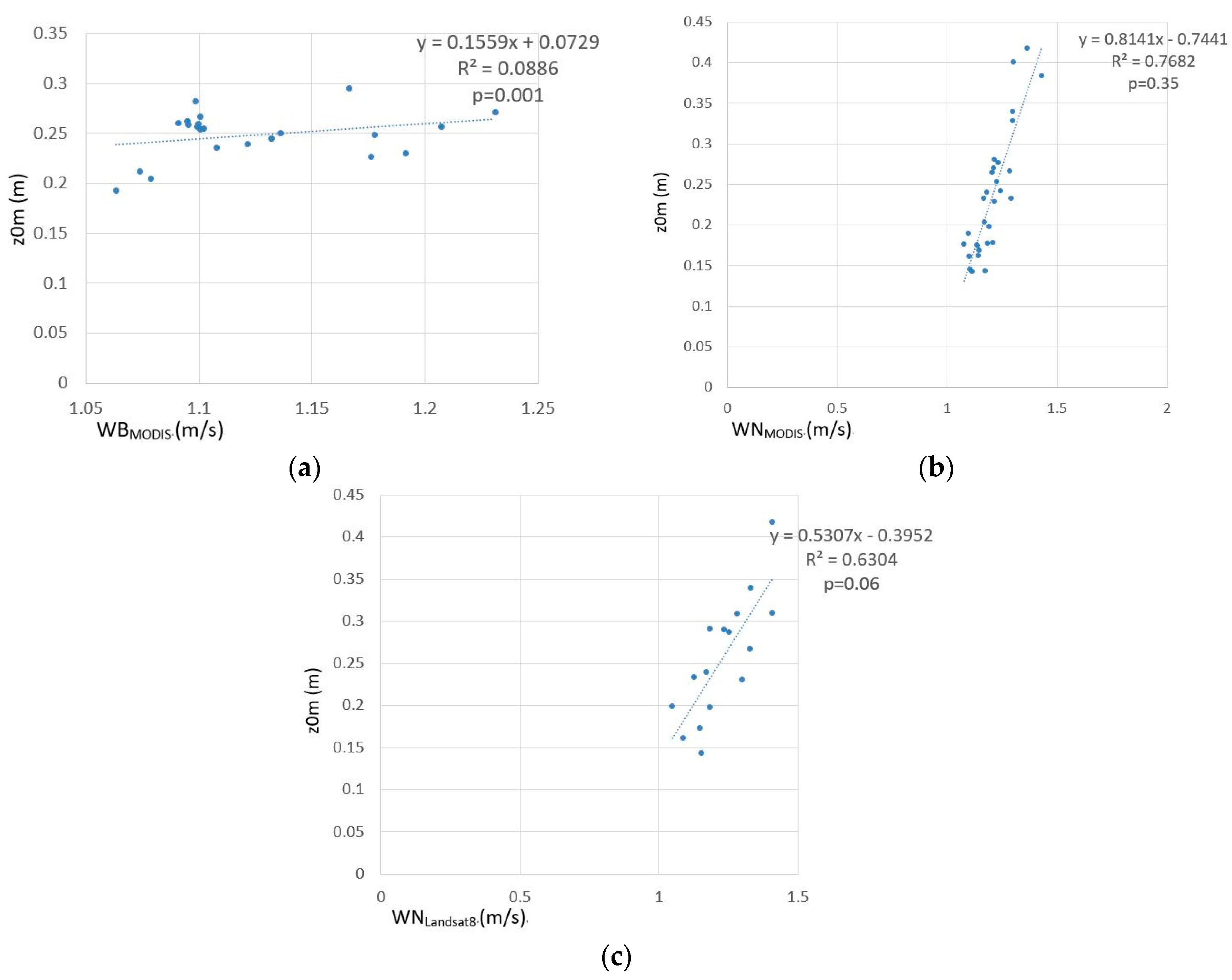
Figure 8.
Regional z0m values in the oasis in the downstream area of the HRB from May to October, 2014 (May 21 (a), June 22 (b), July 24 (c), May, August 16 (d), September 17 (e), and October 12 (f)).
Figure 8.
Regional z0m values in the oasis in the downstream area of the HRB from May to October, 2014 (May 21 (a), June 22 (b), July 24 (c), May, August 16 (d), September 17 (e), and October 12 (f)).


Figure 9.
Footprint estimated at various heights.

Figure 10.
The rose map of z0m with wind direction at Si Daoqiao station.

Figure 11.
The schematic for variation of z0m with wind speed [38].
Figure 11.
The schematic for variation of z0m with wind speed [38].


Table 1.
Observational items and instruments at the Si Daoqiao superstation at 5 m, 7 m, 10 m, 15 m, 20 m, and 28 m [23,24].
| Item | Instrument |
|---|---|
| Air temperature and humidity | HMP45C, Vaisala, Vaisala Oyj, Vanha Nurmijärventie 21, 01670 Vantaa, Finland; AV-14TH, Avalon, 35-1802 River Drive South, Jersey City, NJ 07310, USA |
| Wind speed and direction | 03002, R.M. Young, 2801 Aero Park Drive, Traverse City, Michigan 49686, USA; Windsonic, Gill, Saltmarsh Park, 67 Gosport Street, Lymington, Hampshire, UK |
| Air pressure | Model 278, Setra, 159 Swanson Rd., Boxborough, MA 01719, USA; PTB210, Vaisala, Vaisala Oyj, Vanha Nurmijärventie 21, 01670 Vantaa, Finland |
© 2018 by the authors. Licensee MDPI, Basel, Switzerland. This article is an open access article distributed under the terms and conditions of the Creative Commons Attribution (CC BY) license (http://creativecommons.org/licenses/by/4.0/).
Share and Cite
MDPI and ACS Style
Xing, Q.; Wu, B.; Yan, N.; Yu, M.; Zhu, W. Sensitivity of BRDF, NDVI and Wind Speed to the Aerodynamic Roughness Length over Sparse Tamarix in the Downstream Heihe River Basin. Remote Sens. 2018, 10, 56. https://doi.org/10.3390/rs10010056
AMA Style
Xing Q, Wu B, Yan N, Yu M, Zhu W. Sensitivity of BRDF, NDVI and Wind Speed to the Aerodynamic Roughness Length over Sparse Tamarix in the Downstream Heihe River Basin. Remote Sensing. 2018; 10(1):56. https://doi.org/10.3390/rs10010056
Chicago/Turabian StyleXing, Qiang, Bingfang Wu, Nana Yan, Mingzhao Yu, and Weiwei Zhu. 2018. "Sensitivity of BRDF, NDVI and Wind Speed to the Aerodynamic Roughness Length over Sparse Tamarix in the Downstream Heihe River Basin" Remote Sensing 10, no. 1: 56. https://doi.org/10.3390/rs10010056
Note that from the first issue of 2016, this journal uses article numbers instead of page numbers. See further details here.