Article

Preliminary Study of Soil Available Nutrient Simulation Using a Modified WOFOST Model and Time-Series Remote Sensing Observations

1
Institute of Remote Sensing and Digital Earth, Chinese Academy of Sciences, Beijing 100101, China
2
University of Chinese Academy of Sciences, Chinese Academy of Sciences, Beijing 100101, China
*
Author to whom correspondence should be addressed.
Remote Sens. 2018, 10(1), 64; https://doi.org/10.3390/rs10010064
Submission received: 22 November 2017 / Revised: 27 December 2017 / Accepted: 3 January 2018 / Published: 5 January 2018
(This article belongs to the Special Issue Earth Observations for Precision Farming in China (EO4PFiC))

Abstract

:
The approach of using multispectral remote sensing (RS) to estimate soil available nutrients (SANs) has been recently developed and shows promising results. This method overcomes the limitations of commonly used methods by building a statistical model that connects RS-based crop growth and nutrient content. However, the stability and accuracy of this model require improvement. In this article, we replaced the statistical model by integrating the World Food Studies (WOFOST) model and time series of remote sensing (T-RS) observations to ensure stability and accuracy. Time series of HJ-1 A/B data was assimilated into the WOFOST model to extrapolate crop growth simulations from a single point to a large area using a specific assimilation method. Because nutrient-limited growth within the growing season is required and the SAN parameters can only be used at the end of the growing season in the original model, the WOFOST model was modified. Notably, the calculation order was changed, and new soil nutrient uptake algorithms were implemented in the model for nutrient-limited growth estimation. Finally, experiments were conducted in the spring maize plots of Hongxing Farm to analyze the effects of nutrient stress on crop growth and the SAN simulation accuracy. The results confirm the differences in crop growth status caused by a lack of soil nutrients. The new approach can take advantage of these differences to provide better SAN estimates. In general, the new approach can overcome the limitations of existing methods and simulate the SAN status with reliable accuracy.

Graphical Abstract

1. Introduction

Soil available nutrients (SANs), including available nitrogen (N), available phosphorus (P) and available potassium (K), play an important role in crop growth. Variable rate fertilization (VF), proposed for precision agriculture [1], is an effective method to optimize SAN status at field (based on field survey) or pixel (based on remote sensing data) scales and has been generally accepted on modern farms [2]. With the advancement of mechanized farming and control technologies, the operability and accuracy of VF has been significantly improved. Studies have demonstrated that variable rate fertilization is beneficial to increasing production and revenue, ensuring sustainable agricultural development and protecting the environment [3,4]. A reasonable prescription map is the key factor for VF application [5], and the SAN content is necessary in map making. Hence, the soil nutrient content should be acquired before VF application, and the accuracy of the SAN estimates will decide the application effect. However, timely SAN content monitoring is a very challenging task because of the distribution of the soil plow layer and spatial heterogeneity.
A series of monitoring methods have been designed to obtain soil nutrient content and these can be classified into two types: traditional field surveys and remote sensing methods. Traditional soil testing methods can obtain reliable point-scale results [6], but these methodologies have disadvantages, including high cost and low temporal efficiency, especially when the method is applied at field or regional scales [7]. Remote sensing observations can be used to address these issues and extrapolate simulations over large areas [8,9]. Several studies have confirmed that soil reflectance spectroscopy can be successfully applied to predict soil nutrients [10]. However, because this technique only acquires information from the bare soil spectral reflectance, only the total nutrient content of the soil surface can be measured. This is less useful than the SAN content of the root zone which can provide guidance regarding fertilizer application. By taking advantage of changes in crop growth status caused by a lack of SANs, statistical models can be built by combining the vegetation indexes determined from extensive spatial remote sensing (RS) and SAN content. Such models can overcome the limitations of direct simulations and field surveys by simulating the available nutrients of the whole plow layer, reducing costs, and improving the timeliness of data acquisition [11]. The disadvantages of these statistical models are also obvious. Among them, low stability and simulation accuracy caused by different crop types, study area limitations and application times are typical issues that should be addressed before application.
Crop models can provide the more reliable crop growth parameter simulations because of their comprehensive mathematical descriptions of key physical and physiological processes, simulation of soil processes, and ability to overcome issues such as abnormal weather conditions and natural disasters [12,13]. Furthermore, soil nutrient availability is an important factor used by crop models to simulate crop growth [14]; thus, the changes in SAN content can be easily transferred to the output parameters of crop models. Hence, a crop model could be a feasible model to replace the empirical regression model. However, using a crop model requires the calibration of additional parameters, and the cost is significant, especially when the model is applied at a regional scale. Fully exploiting RS data is useful for addressing this problem. An assimilation method that combines a crop model with time series RS observations (T-RS) can help extrapolate the simulation from a single point to a large area [15,16]. Since Maas first suggested the combining of RS data and modeling in the 1980s [17], several methods for assimilating RS data into crop models have been explored, including the ensemble Kalman filter (EnKF) [13,18,19], particle filtering (PF) [20], and four-dimensional variational data assimilation (4DVar) [21,22]. By assimilating T-RS into a crop model, crop growth parameters can be accurately estimated. Thus, crop models can be used in place of empirical regression models to improve the soil nutrient simulation stability, and they have great potential application prospects.
In this study, we propose a new approach to simulate SAN content in the whole plow layer. The EnKF method is applied to realize crop growth simulation at the pixel scale by integrating the WOFOST model and T-RS observations. The WOFOST model is also modified to build stable connections between crop growth and SAN content. The objectives of the present study are as follows: (1) to verify the feasibility of the new method by analyzing the effects of SAN stress on crop growth, (2) to provide a method for estimating SAN content by connecting the actual and nutrient-limited crop growth simulation results, and (3) to simulate SAN content using the new approach and analyze the simulation accuracy.

2. Materials and Methods

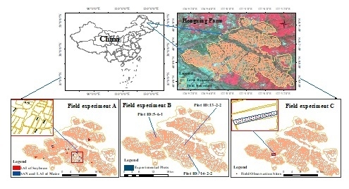
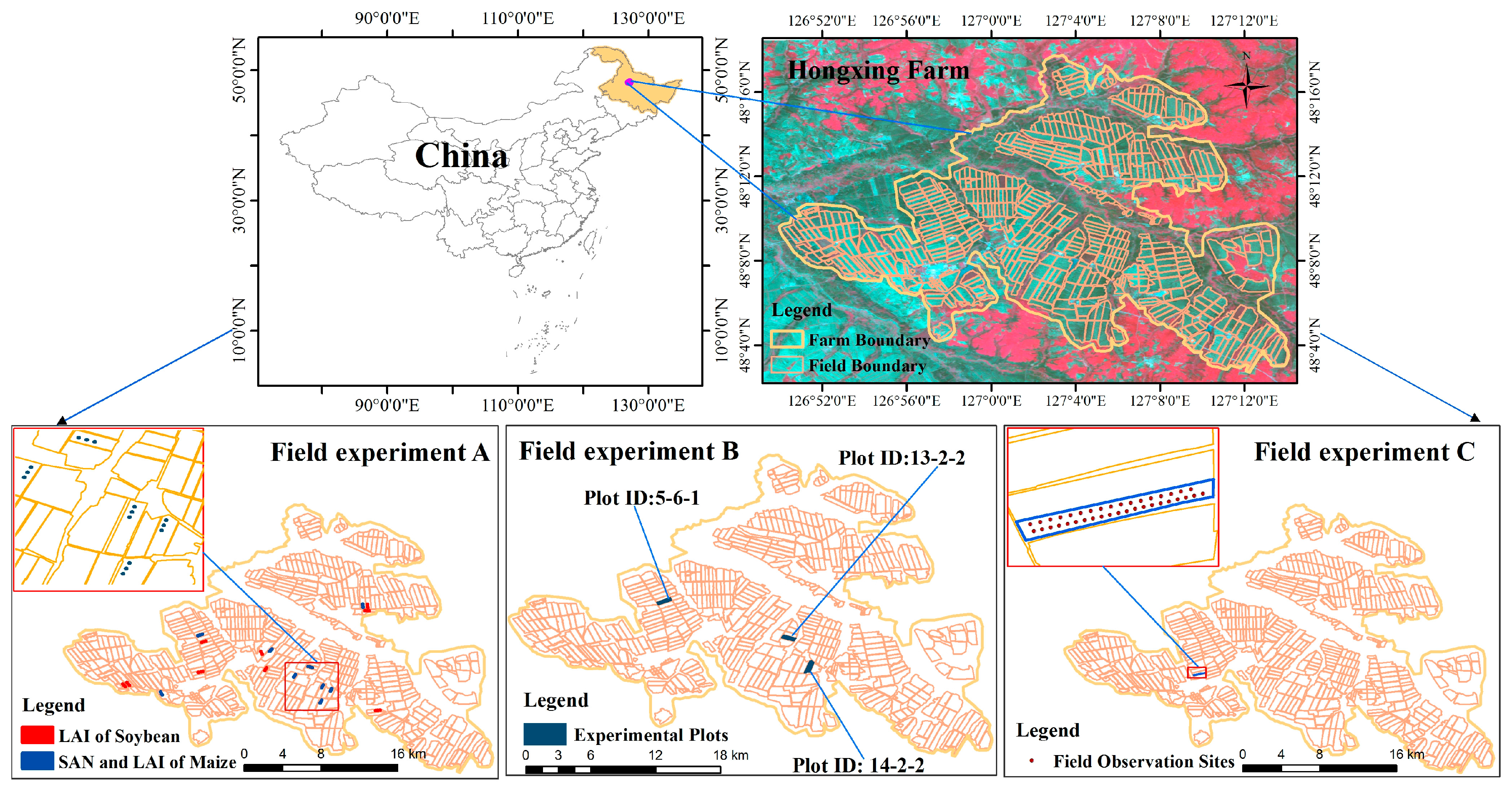
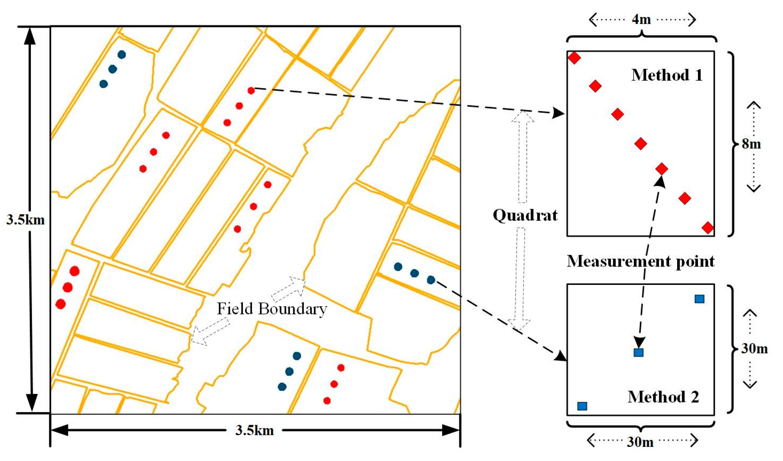
2.1. Study Area and Field Campaign

This study was conducted on a large farm in Northeast China, Hongxing Farm. This farm (48°09′N, 127°03′E) is located in a mid-temperate monsoon climate zone. The average annual precipitation was 548.8 mm and the average annual accumulated temperature (>10 °C) was 2293 °C in 2014. The planting area of Hongxing Farm is approximately 27,300 hectares (ha) and contains 490 plots. The average size of the fields is more than 55 hectares, and moderate-resolution remote sensing data such as HJ-CCD data, which has a spatial resolution of 30 m can easily be applied. The field distribution in this farm is nearly an oblique triangle and a 32 km × 27 km zone covers all arable plots. Spring maize is the major crop and accounts for approximately 50% of the planting area. The soil in this farm is black soil with a depth of 0.5–1.5 m. The fertilizers, including basal dressing, top dressing and leaf fertilizer, are centralized and controlled by the farm department and are applied using modern agricultural machinery. Figure 1 shows the field distribution of Hongxing Farm.
Three field campaigns were conducted in 2014–2015. The locations of these campaigns are shown in Figure 1. During the field campaigns, basic SAN content, the leaf area index (LAI), yield, biomass and nutrient uptake were observed. The sampling strategies included the layout methods for the quadrats and the establishment of the measurement points in one quadrat. Two strategies were used to establish the quadrats: stratified sampling and isometric sampling [23]. The stratified sampling method was used to determine the experimental plots in the study area. Considering the crop type and soil fertility level in Hongxing Farm, the experimental fields were divided into six stratifications: high-nutrient fields, medium-nutrient fields and low-nutrient fields of spring maize and soybean. The cultivation area ratio was calculated by the actual cultivation area of these stratifications. For example, in 2014, the cultivation area of high-, medium-, and low-nutrient fields of spring maize is 8100, 8275, 8150 ha, respectively, and of soybean is 7900, 10,450, 5520 ha, respectively. Then, the cultivation area ratio of the six stratifications is approximately 3:3:3:3:4:2. Using the ratio and the number of experimental plots we planned to select in each experiment, the sampling amount for each stratification could be estimated. The location of the experimental field was labeled on the study area map before the field campaign and minor changes were made based on the actual experimental plots during the field campaign. The isometric sampling method was used to establish quadrats for each plot. Considering the influence of roads and protection forest 200 m away, any edge of the selected plot was used to determine the location of first quadrat. The other quadrats were established using fixed distance along the row crop. Another two sampling methods were used to establish the measurement points in one quadrat, included Method 1 and Method 2 (shown in Figure 2). In Method 1, rectangular quadrats of 4 m × 8 m were established with 7 sampling points in each; the mean values of the points in a quadrat were calculated as the results for that quadrat. In Method 2, considering the resolution of RS data used in this study, the quadrat area was 30 m × 30 m. Three sampling points on the diagonal of each quadrat were selected to gather the objective data.
The three field experiments were designed with different aims: field experiment A was conducted to support LAI simulation model building and accuracy analysis for the SAN content estimations, field experiment B was designed to provide field data for the analysis of the effect of soil nutrient stress on crop growth, and experiment C was conducted in an experimental plot to collect necessary data for SAN uptake equation design and LAI comparison in the discussion section. The details for the three experiments will be introduced in this section. Field experiment A was conducted in 2014 to observe the field LAI and basic SAN content. For the LAI, five sequential field campaigns were conducted in 2014; the observation dates were 10 June, 17 and 25 July, 25 August, and 25 September. The number of quadrats in the first field campaign was 54; thus, we established 9 quadrats in each soil fertility category for spring maize and 9, 12, and 6 quadrats in the high-, medium-, and low-nutrient soybean fields using the stratified sampling and isometric sampling method (the fixed distance was 150 m). The other four campaigns were conducted using a similar sampling method and each campaign was independently conducted with different locations. Two hundred and seventy quadrats across 90 fields were established during the sequential field campaigns and 259 observed LAI were used in this study. LAI-2000 [24,25] and the LAISmart system [26] were used to obtain the LAI field data and Method 1 was used to establish sample points in each quadrat. For LAI-2000, a one-up-seven-down pattern was used to gather the LAI. In each quadrat, we obtained one measurement of sky light above the canopy and then seven measurements of diffuse light below the canopy. The final LAI was measured using an LAI-2000 analyzer. LAISmart was used to correct the errors in the LAI-2000 measurement results where the LAI was lower than 1.0. For the SANs, we measured the basic N, P and K content in the same LAI quadrats of maize plots. The observation time was from 5–9 May 2014. The same quadrats were used for field SAN collection and Method 2 was used to establish the sampling points in each quadrat. At each point, a soil sample to a depth of 40 cm was obtained by using a soil auger. After drying and pulverizing the samples, the SAN content was tested in the lab. Field experiment B was used to analyze the effect of soil nutrient stress on crop growth. Three plots with varying fertilizer rates, including a high-nutrient plot (13-2-2), medium-nutrient plot (14-2-2), and low-nutrient plot (5-6-1), were selected. The SAN content was measured in a field campaign in 2014. Three quadrats were selected using the stratified sampling and isometric sampling methods (the fixed distance was 400 m), and the sampling strategy in each quadrat was Method 2. We calculated the mean value of the nine sampling points as the SAN content of the experiment plot. After harvesting was completed, we obtained the total weight of each plot, and the yield was estimated by dividing the total weight by the area. The soil nutrient uptake and the biomass of maize in different growth periods were necessary to build the uptake equation; these data were gathered in field experiment C. In this experiment, we selected an experimental plot (5-1-2) and established 37 sampling quadrats. The isometric sampling method (the fixed distance was 100 m) was used to establish these quadrats. For each quadrat, we obtained the biomass and SAN uptake amount of two maize plants by drying, weighing and testing the plants in the lab. The sampling strategy is similar to Method 2 while the quadrat area was 10 m × 10 m. Field experiment C was conducted in 2015, and sampling was performed on eight dates: 27 May, 13 and 24 June, 20 and 28 July, 29 August, 5 September and 8 October. Furthermore, LAI was also measured in this plot using LAI-2000 and LAISmart. The sampling strategy was Method 1 and the observation times were 27 June, 31 July and 30 August.

2.2. RS Data and Processing

We selected time series HJ-1A/1B CCD data to simulate soil available nutrients. The data were collected from two Chinese environmental RS satellites: HJ-1A and HJ-1B. There are four advantages to employing such RS data in this study: broad coverage (360 km), a frequent revisit period (2 days), moderately high spatial resolution (30 m), and appropriate spectral resolution (four visible and near-infrared bands: 430–520 nm, 520–600 nm, 630–690 nm, and 760–900 nm). We obtained 15 images of Hongxing Farm in 2014 for the following dates: 13 and 29 April; 24 and 31 May; 12 and 22 June; 7, 14 and 26 July; 19 August; 12, 18, 24 and 30 September; and 4 October. The images were obtained from the China Centre for Resources Satellite Data and Application (CRESDA) site (http://www.cresda.com/EN/gywm/zxgk/index.shtml). Relative radiometric correction and systematically geometric correction [27] were performed by CRESDA before data sharing. Precise geometric correction was applied to the CCD images based on the Landsat TM 5 image of the study area. Fifteen field-measured ground control points were used to calculate the root-mean-square error (RMSE) of the corrected CCD images. The results show that the RMSE was less than one pixel (30 m) for the acquisition time from April to October. The universal transverse Mercator (UTM) 50N projection was used for each image. The radiometric calibration coefficient and spectrum response function (SRF) were provided by CRESDA and used to perform atmospheric correction. The Fast Line-of-Sight Atmospheric Analysis of Spectral Hypercubes (FLAASH) model in the ENVI software (version 5.3) was used to realize the atmospheric correction [19,28]. The normalized differential vegetation index (NDVI) was used to estimate the LAI, and the NDVI can be expressed as,
N D V I = N I R R E D N I R + R E D
where NIR and RED are the reflectance of the near-infrared band (760–900 nm) and red band (630–690 nm), respectively.

2.3. WOFOST Model

Crop models can provide reliable crop growth simulations because of their comprehensive mathematical descriptions of key physical and physiological processes, simulation of soil processes, and ability to overcome issues such as abnormal weather conditions and natural disasters [12,13]. Furthermore, soil nutrient availability is an important factor used in crop models to simulate crop growth [10]; thus, crop models can be used to improve the stability and accuracy of common SAN simulation methods. The WOFOST model was selected to replace a statistical model in this study.
The WOFOST model [29] used in this study was built by the Center of World Food Studies located in the Netherlands, more than 15 years ago. The model is a popular eco-physiological model worldwide and can simulate daily crop physiological and ecological processes, including CO2 assimilation, respiration, leaf growth and dry matter formation. The soil nutrient module was an important factor contributing to our selection of the WOFOST model. This module can simulate the uptake of soil nutrients, the use of crop nutrients, and nutrient-limited crop parameters. It is the key module utilized in SAN estimation. Using the soil nutrient module, the nutrient-limited yield can be estimated based on the potential or water-limited yield. In this study, all the values of nutrient-limited yield and crop growth were estimated based on water-limited results. The widespread application of the WOFOST was another factor leading to our use of this model. The main parameters of the WOFOST model have been well calibrated for different crops under different meteorological, soil and management conditions via field campaigns and RS data assimilation in China [13,14]. However, crop parameters can vary substantially among different types of spring maize. Hence, a new calibration was necessary.

2.4. T-RS Observations Assimilation

Crop growth parameters are required by the SAN simulation. We used the WOFOST model to perform the simulation. However, the WOFOST model was originally designed for point-based simulation. Thus, additional parameters should be calibrated when using the model to simulate crop growth at the regional scale, and the costs must be considered. An assimilation method that combines a crop model with T-RS observations can help extrapolate simulations from a single point to the regional scale.
LAI is the main daily output variable of the WOFOST model, and it is the key factor in light capture and carbon assimilation. In this study, we selected LAI as the index in the data assimilation procedure. Hence, a time series of RS-based LAI should be estimated before assimilation. Previous studies have shown that several methods can be used to accurately estimate LAI from RS data. Among them, physical model-based methods [30,31] and empirical regression methods [32] are frequently used. Previously, we compared the accuracy of a PROSAIL model (physical model-based method) with that of a simple empirical regression model (empirical regression method) [33]. The results indicate that the empirical regression model can provide more accurate LAI simulation than the PROSAIL model. In the present study, we focused on the feasibility and accuracy of SAN estimation based on the difference of two types of LAI results. The LAI simulation accuracy was the main factor leading us to select the model. Therefore, we used the empirical regression model to realize the RS-based LAI simulation.
The EnKF method [34] was used to assimilate the LAI estimates into the WOFOST model. The EnKF method is based on Monte Carlo ensemble generation and performs model forecasting with two related parts—the model dynamics and a filter update—to realize assimilation [14]. The core algorithm is shown in the following equation:
A a = A f + A c H T ( H A c H T + D c ) 1 ( D t H A )
where Aa is the optimal estimated ensemble, Af is an ensemble of forecast, K =   A c H T ( H A c H T + D c ) 1 is the Kalman gain matrix, Dt is an ensemble of observation, and HA is typically equal to 1.
The EnKF was applied at the pixel scale independently. For each pixel (30 × 30 m), the EnKF algorithm integrates the RS-based LAI and model-simulated LAI to generate the forecast ensemble [14]. The result ensemble was used as the input LAI in the next step of model crop growth simulation. The assimilation process was repeated until the required end time is reached. Furthermore, an expansion parameter (E) was used to solve the filter divergence problem.

2.5. WOFOST Model Modification

The SAN content can influence crop growth through four aspects: crop cell formation, carriers, enzyme activity change, and information transmission. For example, the soil available nitrogen maintains the chlorophyll level and increases its activity; thus, this nutrient may play a more important role during the rapid growth phase of the crop biomass than during other phases, and the optimal simulation time for soil available nitrogen is generally the early growth season. Furthermore, the period of SAN simulation and fertilization and its effects on application cannot be ignored. Thus, the nutrient module should be applied during the growth season. Because the original model only allows us to use the nutrient module at the end of growth season, necessary model modification must be performed before SAN simulation.
To facilitate the modification, we recoded the WOFOST model with interactive data language (IDL) and reintegrated the modules. The original module calling queue of daily crop growth simulation is emergence time, CO2 assimilation, transpiration, soil water, water stress, respiration, dry matter formation, biomass increment, LAI and remote sensing assimilation. The yield and soil nutrient module are applied at the end of crop growth season to estimate water- and nutrient-limited yield, i.e., nutrient-limited crop growth can only be estimated at the end of crop growth simulation. In the rewritten code (IDL-WOFOST), we can change the module calling sequence and add the soil nutrient module to the end of the daily simulation calling queue. This allows mid-season nutrient-limited crop growth to be simulated in the IDL-WOFOST model. Because performing nutrient-limited crop growth simulation for the whole season will increase the running time, the module calling sequence was changed at the required time during the growth season in this study.
The daily nutrient uptake of spring maize can be influenced by crop growth condition, soil compaction, soil water content, and fertilization [35,36,37,38,39]. As the original WOFOST model calculates the seasonal nutrient supply, variation is ignored, which is unproblematic for the nutrient-limited yield estimation at the end of the growth season. However, errors are inevitable when the new module calling sequence is applied to within-season nutrient-limited crop growth simulation. Therefore, within-season soil nutrient absorption is another problem that should be addressed before the new module calling queue is applied. In WOFOST, the absorption fraction of spring maize is 1 when the growth period is 120 days and 0.55 when the growth period is 60 days. However, the absorption fraction cannot simply be considered 0.55 when the nutrient module is called on the sixtieth day of the growth season, which is more than 60 days. Generating the soil nutrient absorption rate curve of spring maize is necessary to address this problem. Previous work has shown that the rate of soil nutrient absorption for maize is low in the early growth season; it then rapidly rises and then gradually declines [40]. The process approximately follows an S-curve and can be simulated by an exponential equation:
D ( t ) = a t 2 e c t
where D(t) is the soil nutrient absorption rate, t is the day of the growing season (DOG), and a and c are coefficients that should be calibrated when the crop variety is changed.
Furthermore, we combined the SAN content and fertilizer amounts as the total SAN input parameters of the nutrient module. However, the basic unit of nutrients measured during the field campaign (mg/kg) is different from the WOFOST model input nutrients and fertilizer application (kg/ha). The following equation is used to convert the relevant units:
N s o i l = N a c t u a l 10 6 ρ h 10 4
where ρ is the soil density, Nactual is the nutrient content measured during the field campaign, and h is the effective soil depth, which is the minimum depth of the root and soil in the field campaign data.

2.6. SAN Simulation Algorithm

Based on the model modification, the mid-season SAN absorption amounts and their influence on crop growth can be estimated. We designed a series of corresponding algorithms to realize the SAN simulation. To express the SAN simulation clearly, the process of crop growth simulation in the WOFOST model was divided into three stages: pre-growth stage, SAN simulation stage, and late growth stage. First, the WOFOST model was used to simulate crop emergence and early crop growth in the pre-growth stage. Then, the SAN content was estimated in the second stage. Based on the SAN estimates, the nutrient-limited yields were calculated based on the SAN simulation results in the late growth stage. In the SAN simulation stage, the T-RS observations obtained at the start (point A) and end (point B) of this stage were assimilated into the WOFOST model using the EnKF method to estimate the actual short-term crop growth. Additionally, WOFOST simulates the nutrient-limited crop growth at point B using the nutrient module. The two types of crop growth simulations should yield similar results if the soil nutrient input parameters are well calibrated at the pixel scale. However, this process is difficult because of the spatial heterogeneity and variability of the SAN content. Nevertheless, we took advantage of the errors in the nutrient-limited crop growth simulation and applied algorithms to monitor the SAN content.
During the SAN simulation, we varied the nutrient input parameters within a large scope and included all probable values. The nutrient-limited growth was then calculated at different levels. Via comparison with the actual growth simulation results, the objective results were determined. Because the nutrient module should be repeated for all the probable input SAN values at the pixel scale, the time cost is large. Thus, the SAN simulation algorithm was designed to be similar to the look-up table (LUT) method. The table was built by the input variables and output results from the soil nutrient module. Moreover, considering the varying functions and key function periods of different nutrients, we set the other two nutrients at the mean level of the whole farm when the third nutrient was simulated. For example, when we estimated N content, P was 40 mg/kg and K was 176 mg/kg, which were both equal to the mean values of Hongxing Farm. Based on the field campaign data, the N in the table was between 0 kg/ha and 1000 kg/ha with an interval of 0.1 kg/ha. Then, the DOG was varied to include all the possible times of point A and point B, and the corresponding SAN uptake amounts were calculated. The SAN uptake estimation also considered the SAN consumption of the dead biomass. The dead biomass can be simulated by the WOFOST model, and the SAN percentage of this part was equal to the normal biomass. In addition, the water-limited leaf, stem and storage organ biomass of point A and point B and the water-limited LAI value of point B were added to the table. Their ranges of variation were determined by the field data to ensure that all the input biomass combinations were included. Running the nutrient module with the input SANs, LAI and biomass information, the nutrient-limited biomass and LAI can be estimated. The table includes N contents, effective soil depth (Equation (4)), DOG, input water-limited biomass combinations, and output nutrient-limited LAI. Three tables for the N, P and K simulation were made independently, and nine lines of the N table are listed in Table 1.
When the N content is simulated at point B, the input biomass of point A and point B and the input LAI of nutrient module are provided by the crop growth simulation process in the WOFOST model. The P, K, fertilization and DOG are fixed values. As a result, 1000 lines with different N and output LAI combinations can be selected from the table. Via comparison with the RS-based LAI, the ideal N content can be found. P and K can also be simulated by using a similar method. The LUT method can help us to avoid running the nutrient module for each pixel. The process of crop growth and SAN simulation is shown in Figure 3.

3. Experimental Results

The new approach estimates SAN content through three processes. In the first process, T-RS observations are assimilated into the WOFOST model using the EnKF method to estimate actual crop growth. In the second process, WOFOST is modified to estimate nutrient-limited crop growth by combining the simulation results of water-limited crop growth and the soil nutrient module. In the third process, SAN simulation algorithms are designed by comparing the actual and nutrient-limited crop growth. The complete results of model calibration, LAI estimation and soil nutrient absorption equation calibration are presented in this section. Then, the SAN simulation method was conducted in the spring maize fields of Hongxing Farm. We also analyzed the effect of soil nutrient stress on crop growth, the simulation accuracy of crop growth, the SAN simulation accuracy and the application potential in this section.

3.1. Calibration of WOFOST Model

There are more than 80 input parameters in the WOFOST model, including meteorological, soil, and crop parameters. Daily meteorological data, including temperature, sunshine duration, wind speed, vapor pressure, precipitation, and humidity were available from the meteorological station in Hongxing Farm as the meteorological parameters. The soil and crop parameters needed to be calibrated by field campaigns. Before parameter calibration, the sensitivity was analyzed. Because LAI was selected as the index to realize the RS data assimilation and SAN simulation, we analyzed the sensitivity of the input parameters. Moreover, the nutrient-limited LAI, which is simulated in the modified WOFOST model (described in the following section), was selected as the index to realize the analysis. Because LAI is a daily output parameter in the WOFOST model, the development stage of the crop (DVS) was also considered, and DVS = 0.5, 1.0, and 1.5 were used to give the time of output LAI. We varied the soil and crop parameters from 95% to 105%, and the variations in output LAI were calculated by the WOFOST model. The reason we selected 95% to 105% as the variation in this study was to guarantee all the parameters keeping in a reasonable range. Then, the sensitivity factor (Sfactor) was calculated by the following equation,
S f a c t o r = L A I Δ p a r a m e t e r p a r a m e t e r Δ L A I
where LAI is the mean LAI simulation results of DVS = 0.5, 1.0 and 1.5, parameter is the input parameter value, parameterΔ is the variation of the input parameter, and LAIΔ is the mean variation of LAI along with the parameter variation. Sfactor is a non-dimensional ratio, and the sensitivity judgment standard is listed in Table 2.
Based on the Sfactor value and judgment standard, we calculated the sensitivity values of the crop and soil parameters. The results indicate that 21 parameters show sensitivity to highly significant sensitivity to the LAI (Sfactor is equal or greater than 0.2), and we calibrated them by the field campaigns in this study. The values of the sensitivity parameters are listed in Table 3. Details of the calibration methods can be found in our previous study [31].
We applied the original and calibrated WOFOST model to simulate spring maize growth in 2014 and analyzed model performance. Emergence time, anthesis time, maturity time and yield were selected as the indexes to assess the parameter simulation accuracy. These parameters were simulated at pixel scale, and then averaged them as the value for the whole farm. The analysis results are listed in Table 4 and indicate that the calibrated model accurately simulated spring maize crop growth. The errors of simulated emergence time, anthesis time, maturity time and yield were −2 days, 3 days, 2 days and −40.50 kg/ha, respectively. Compared with the original model, the calibrated model showed the improved simulation accuracy.

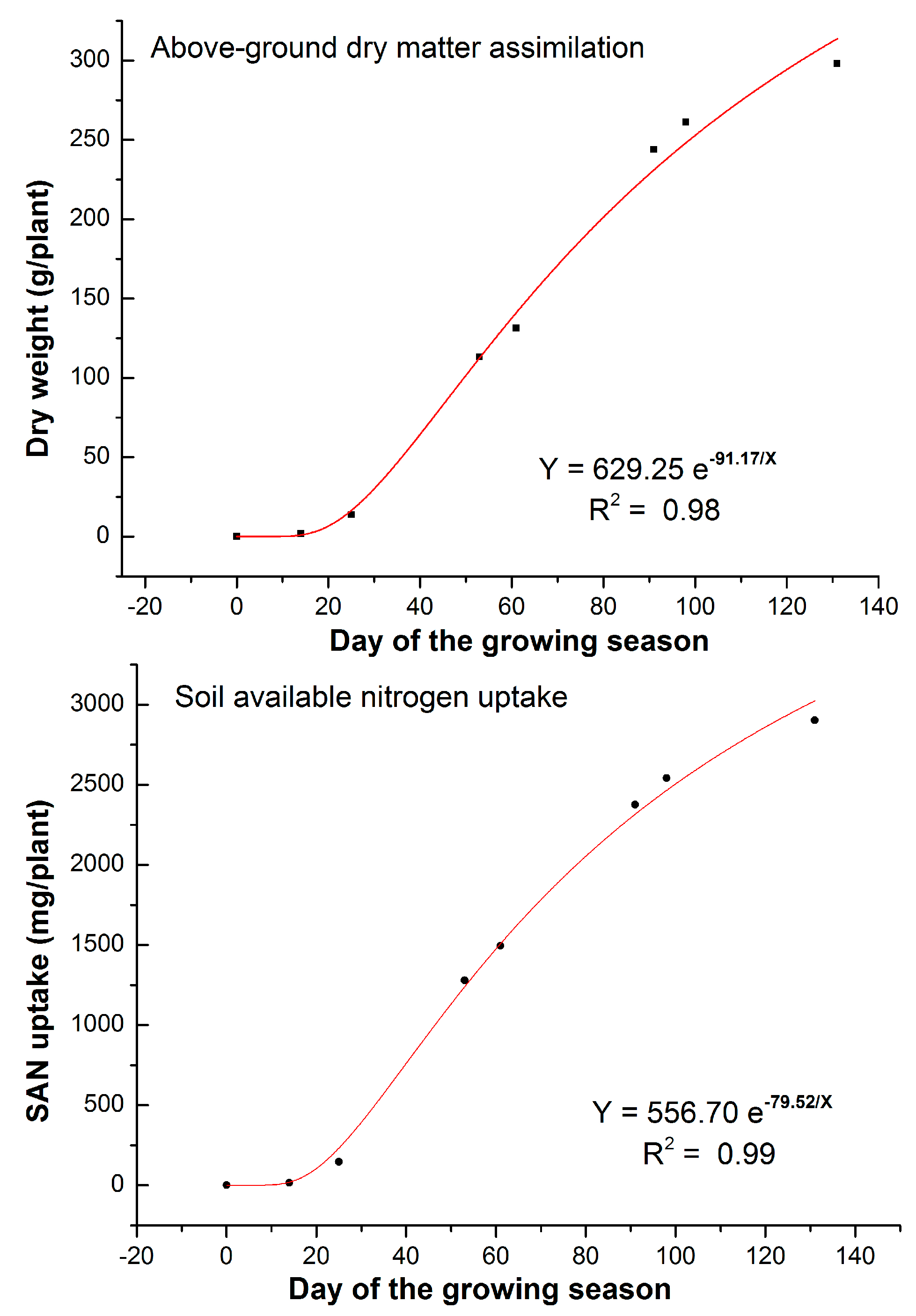
3.2. Calibration of Soil Nutrient Absorption Equation

Equation (5) should be verified and recalibrated before it is used to simulate the daily SAN absorption amount. We conducted a field campaign (field experiment C) for verification and calibration. The mean biomass of the 37 sampling points was calculated as an index to analyze the quantitative relationship between biomass and the DOG. Then, the mean SAN uptake value was calculated and analyzed. The analysis results (shown in Figure 4) indicate that the biomass assimilation and SAN uptake amount show a similar pattern and can be estimated by an exponential curve.
From Figure 4, we find that the N uptake amount can be simulated by
N ( t ) = 556.70 e 79.52 t
where N(t) is the soil nutrient absorption rate, and t is the DOG. The N absorption rate can be calculated by the derivative of Equation (6), which is similar to Equation (5),
D ( t ) = 44268.78 t 2 e 79.52 t
Using Equation (7), the total N uptake amount of a maize plant at time t can be estimated. For the amount from t1 to t2, we can integrate Equation (8),
N t = t 1 t 2 44268.78 t 2 e 79.52 t d t
However, the SAN uptake estimation is for a single maize plant. Additional coefficients should be added to Equation (8) to extrapolate the estimation to the field scale. We introduced the coefficient Cfarm to realize the unit conversion from mg/plant to kg/ha. Cfarm can be estimated based on the plant density. Furthermore, another coefficient, CLAI, was added to Equation (8) to incorporate the influence of crop growth status. CLAI is computed as
C l a i ( t ) = L A I ( t ) L A I 0 ( t )
where LAI(t) is the LAI of the target plot or pixel at time t, and LAI0(t) is the mean LAI value of the experimental field at time t. The crop absorption can be given by
N u p t = t 1 t 2 C f a r m C l a i a t 2 e c t d t
where Nupt is the soil nutrient absorption (kg/ha) at time t. Equation (10) can be used to simulate the SAN uptake of the study area at the field scale. However, the growth period is variable for different meteorological conditions and planting plans. In 2015, the emergence time was 27 May, and the growth period was 135 days, whereas in 2013, heavy snow caused waterlogging and delayed the sowing time, decreasing the growth period to 122 days. Hence, the DOG cannot be directly put into Equation (10). The DVS can be used to unify the growth period of different years. In the WOFOST model, the DVS is calculated from the thermal time and DOG:
D V S ( t ) = 1 t D T U M ( t ) T S U M
where DVS(t) is the DVS when DOG is t, DTUM(t) is the effective accumulated temperature of the corresponding time, and TSUM is the total required thermal time from emergence to harvest. For 2013, when we calculate the N uptake amount at a DOG of 60, the DVS is 0.90. Inserting DVS = 0.90 into Equation (11), the DOG can be estimated as 67. Accordingly, we should put t2 = 67 and t1 = 1 into Equation (10) when the N uptake from the beginning of the growing season to DOG = 60 in 2013 is required. The P and K uptake can be simulated by similar equations, and the coefficient values are listed in Table 5.

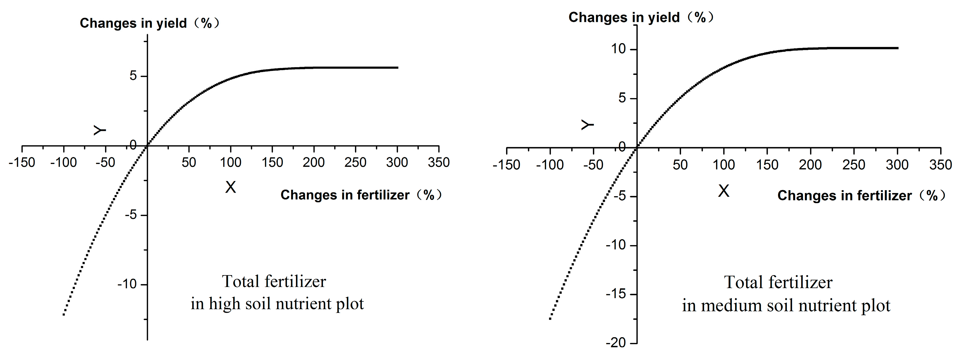
3.3. Effect of Soil Nutrient Stress on Crop Growth

The precondition of the new SAN simulation method is the difference between the RS-based actual crop growth and WOFOST-based nutrient-limited crop growth. Hence, showing that changes in current SAN content can affect crop growth is necessary before designing the simulation algorithm. We first analyzed the effect based on the field campaign results; then, the effect on model crop growth simulations was assessed by running the WOFOST model under different SAN conditions.
A series of variable rate fertilization experiments have been conducted in Hongxing Farm for more than ten years, and the resulting experimental data are useful for analyzing the soil nutrient stress. In Hongxing Farm, the fertilizers include carbamide (CH4N2O), diammonium ((NH4)2HPO4) and potassium sulfate (K2SO4). The three fertilizers were mixed in a fixed proportion and applied to the field. The ratio of N, P and K of the mixed fertilizer was 17:12:9, which is controlled by the farm. In 2010, a spring maize plot covering 12 hectares (ha) was selected as the experimental field. The field was divided into two parts: 9 hectares (part A) with normal fertilization and 3 hectares (part B) with variable rate fertilization. The fertilizer amount in both parts was 700 kg/ha. Here, normal fertilization means that 6300 kg fertilizer was uniformly used in part A. For part B, a reasonable prescription map was made based on the SAN field measured data, then the variable rate fertilization was applied. The average yield of the two fields were gathered at the same time. The average yield of the variable rate fertilization part increased from 8905 to 9735 kg/ha. This finding indicates that optimizing the fertilization can increase the yield. To illustrate the influence directly, we designed an experiment that was conducted in another spring maize plot in 2014. The 71-hectare plot was divided into three parts, and different fertilizer amounts were applied in each part. Then, the yields of the three parts were measured. The results (listed in Table 6) show that changes in the fertilizer amount can directly influence the yield. Considering the relationship between crop growth and yield, we can conclude that changes in SAN content can cause variation in crop growth in the study area.
We also analyzed this stress through WOFOST model simulation. Fertilization and simulated yields were selected as indexes to test whether soil nutrient stress can influence the WOFOST-based crop growth simulation. In field experiment B, we selected three plots to observe the SAN content and yield. We also simulated the mean yield with the WOFOST model and RS data. Details of these plots are listed in Table 7.
The soil nutrient stress on crop growth was analyzed by a simple method. In this method, the total N, P and K fertilizer applications were varied from −100% to 300% in 2% increments, and the WOFOST model was repeatedly executed at each step to simulate the yields at different fertilization levels. The output yields (shown in Figure 5.) indicate that any change in the fertilizer application can initiate differences in the crop simulation process. In general, the changes in SAN content can affect crop growth, and the calibrated WOFOST model can be used to simulate these changes.

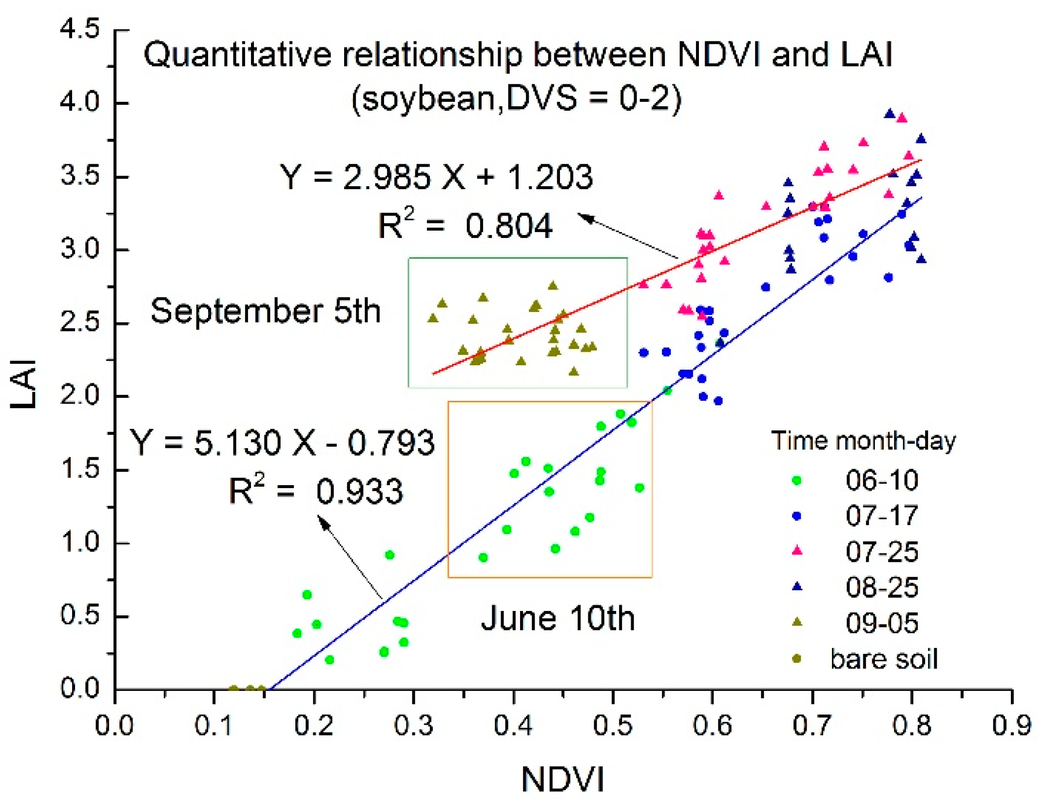
3.4. Crop Growth Simulations
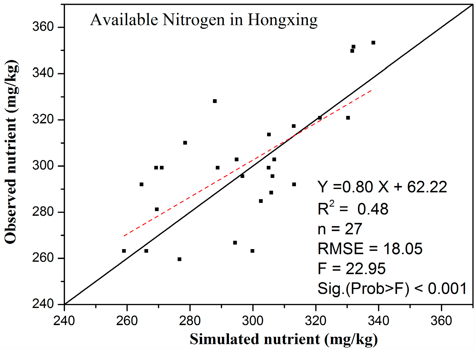
The T-RS observations and modified WOFOST model were used to estimate the required actual crop growth and nutrient-limited growth. An empirical regression model was used to estimate LAI from the T-RS observations. In field experiment A, we obtained the field LAI of maize and soybean. The empirical regression model was constructed using NDVI and field campaign data. The NDVI and LAI of one crop showed similar trends of initially increasing and then decreasing, whereas the rate did not remain the same. Hence, the relationship between the NDVI and LAI varied. This phenomenon became evident when we analyzed the field LAI of soybean. The results, which are shown in Figure 6, show that a given NDVI value corresponds to two different LAI values, one from an earlier stage of the growing season and the other from a later stage.
It was necessary to address this problem before building the model of spring maize. Therefore, the DVS was considered. DVS = 1, i.e., when the LAI reached its peak value, was considered as the limit for both stages. The empirical regression models and the accuracy of spring maize are listed in Table 8. Previous work has shown that the RS-based LAI can be easily assimilated into the WOFOST model [19]. A physical model, such as a PROSAIL model, is still recommended when the SAN simulation method is applied to a larger area or a longer time span.
In addition, the LAI and yield were selected to analyze the simulation accuracy. For actual growth, the EnKF method was used to assimilate time-series HJ-CCD data into the WOFOST model to correct the model crop growth simulation process. The water-limited LAI of WOFOST and RS-estimated LAI are typically selected as the indexes used for assimilation. However, because of the existence of nutrient stress on crop growth, the water-limited LAI of the original model is higher than that of the RS-simulated result, as shown in Figure 7. Thus, the assimilated LAI is higher than the RS-based LAI, which can influence the SAN simulation. In this study, we calculated the mean nutrient-limited LAI using the mean SAN content of the entire farm, and the mean nutrient-limited LAI was used to replace the water-limited LAI for the RS assimilation. The LAI profile (shown in Figure 7) shows that this substitution can improve the LAI assimilation accuracy. Additionally, we conducted a field campaign in 2014 to gather the mean value of yields. In this campaign, 134 spring maize plots were selected, and the details of plot location and yield observation method can be found in our previous study [30]. The coefficient of determination (R2), root-mean-square error (RMSE) and average relative deviation (ARD) were selected as the indexes to analyze the accuracy of the yield simulation based on the WOFOST model and the EnKF assimilation method. The results (shown in Figure 7) indicate that the simulation accuracy (R2 = 0.58, RMSE = 530.61, ARD = 4.45%) of the WOFOST model with the EnKF method is higher than the original model (R2 = 0.13, RMSE = 976.53, ARD = 9.17%).
For nutrient-limited growth, the daily crop growth parameters were first simulated by the WOFOST model at the water-limited level. During the model modification process, the nutrient module was added to estimate the nutrient-limited crop condition parameters based on the water-limited results. Because the SAN content cannot be acquired at the pixel scale, the soil nutrient parameter inputs were generated from 27 sets of field data using kriging interpolation, thus, some associated errors are inevitable. R2 was selected as the index to analyze the difference between actual and nutrient-limited crop growth. The analysis results (listed in Table 9) indicate that the simulation accuracy of actual growth is higher than that of nutrient-limited growth. Using the errors associated with nutrient-limited growth compared with those of the actual growth, we can design algorithms to simulate the SAN content.

3.5. SAN Simulation

A preliminary attempt at SAN simulation was made in the spring maize plots of Hongxing Farm, and analyses were conducted to assess the accuracy. The SAN simulation algorithm was used in the soil nutrient simulation stage to create a connection between actual crop growth and nutrient-limited growth. The ranges of N, P and K were set to 0–1000, 0–200, and 0–700 mg/kg, respectively, to include all possible SAN content. The time of point A was DVS = 0.12 to ensure the spring maize emergence. Moreover, the change at point B corresponds to different periods of assimilation and crop growth stages. Hence, we varied the time of point B from DOG = 23 to 123 with a step of 10 and repeated the simulation process to estimate a series of SAN content. The R2 values of these simulation results were calculated. The results indicate that the change at point B can have significant effects on the simulation accuracy. We selected the optimal time for the three nutrients according to the R2 values. Specifically, the optimal time for N was 43 (DOG), and the accuracy is shown in Figure 8. The results indicate that this method can simulate the spatial heterogeneity of N with acceptable accuracy (R2 = 0.48). Similarly, the optimal times for P and K are DOG = 53 and 63, respectively.
Additionally, a commonly used method was applied by building a statistical model using the RS index and SAN content. We selected the optimal index and time by performing an accuracy analysis. The near-infrared (NIR) band of the RS image on 22 June (DOG = 23) simulated N content with the highest R2. In addition, the NDVI and ratio vegetation index (RVI) of the RS image on 19 August (DOG = 57) were optimal for the determination of P and K. Finally, the R2 values of the two different methods were calculated. The results, which are listed in Table 10, show that the new approach can monitor the SAN content with higher accuracy than can the statistical model.

3.6. The Application Value of the SAN Simulation Algorithm

The aim of SAN estimation is to generate a prescription map for guiding VF. Hence, in this study, it was important to analyze the improvement that the new SAN simulation method can provide in VF applications, and we discuss this in this section. The VF experiments (introduced in the previous section) demonstrated that yield can be improved by controlling fertilization. However, these experiments were conducted based on field campaign data. The spatial heterogeneity of soil nutrients and the errors from the spatial interpolation in the prescription map can both lower the application effect. We applied the new SAN simulation method to improve the application value by providing timely SAN content information at the pixel scale. The three plots of field experiment B were selected to analyze the improvement. Considering that the VF method of the previous experiments involved maintaining total fertilization while boosting yield, the fertilization rate of the three plots was set to 700 kg/ha. We produced the prescription map and ran the WOFOST model to obtain the yield increase. The results (listed in Table 11) indicate that the new method can improve the mean yield of the three plots from 10,304.90 to 11,428.51 kg/ha with an increment of 1123.61 kg/ha. Meanwhile, the increment of the VF experiment in 2010 was 830.00 (from 8905.00 to 9735.00) kg/ha. Hence, the new method can provide a greater yield growth than the field survey method with the same VF strategy. In general, the new method is promising for optimizing SAN content, which can increase production and ensure sustainable agricultural development.

4. Discussion

Previous research has demonstrated that it is feasible to simulate soil nutrients using different methods, which have been mainly adopted from field surveys, soil spectroscopy and remote sensing. However, these methods have obvious shortcomings, and many of them may pose an obstacle to simulating results for fertilizer management on a larger scale. Field surveys are inefficient and costly, soil spectroscopy can only monitor the total nutrients from the surface soil, and remote sensing usually adopts statistical methods and cannot guarantee precision and stability. Therefore, in this study, a model with a more thorough theoretical basis and a more stable framework was evaluated, and its soil nutrient module can represent soil nutrient content with the input of remote-sensing data assimilation, and soil nutrient simulation methods. Compared with typical methods, this model has obvious advantages in particular, low cost, timeliness, and precision.
In terms of cost, the HJ-CCD data used in this study is free on the internet, and the field data was gathered only to calibrate parameters and analyze nutrient simulation accuracy. It was unnecessary for us to conduct field surveys and soil sample assays for each year; hence, the cost of this method is lower than that of field surveys and soil spectroscopy. In terms of timeliness, the revisiting period of HJ satellites is two days and the CCD cameras observe broad coverage of 360 km. This capability gives us more options in this method than others. In terms of precision, the application of WOFOST provides a more robust theoretical basis and detailed mechanism process. Also the nutrient module of this method is able to consider the influence between different nutrients. This can improve the precision of nutrient monitoring and the accuracy analysis results has verified the improvements.
The error propagation of the proposed SAN simulation was also analyzed in this study. Considering the SAN content was simulated by comparing the difference of WOFOST based LAI and the RS-WOFOST based LAI (the LAI simulated by assimilating time-series LAI into WOFOST model), any errors in the RS-WOFOST based LAI can influence the SAN simulation accuracy. Hence, we selected the RS-WOFOST based LAI as the index to analyze the error propagation of the proposed SAN simulation model. The mean value of RS-WOFOST based LAI were varied from −90% to 100% in 5% increments. The SAN simulation method was repeatedly executed at each step to calculate the changes in N, P and K estimations. The results, listed in the Table 12, indicate that the error propagation from RS-WOFOST based LAI to SAN simulations matches an approximate linear relation.
Meanwhile, this study is a preliminary study. Some deficiencies should be addressed before the new method can be used to guide VF application. Among these, the K simulation accuracy is important. The analysis results showed that the accuracy of K is lower than that of N and P for both methods. There are several potential reasons for this finding, which can be classified into four aspects: the stability of K in soil, the absorption-action mechanism of K in spring maize, the interaction effects between SANs, and the RS assimilation effect. The potassium ion is the main form of K in soil, which means that it can be easily influenced by soil water flow. The spatial heterogeneity of SAN content was analyzed and a variable coefficient (CV) was selected to examine the spatial heterogeneity. The CV can be calculated as [30]
C V = S D M e a n 100 %
where SD is the standard deviation and Mean is the mean value of the research data.
We calculated the CV values of the field SAN content data in the nine selected plots of field experiment A. Then, the mean value of them was estimated and the spatial heterogeneity of K (CV = 11.70%) was found to be higher than for N (CV = 4.53%) and P (CV = 10.48%). The results indicate that K is more readily changed than N and P. For the absorption-action mechanism of K in spring maize, K plays an important role in crop metabolism, protein synthesis and charge balance [41]. In this study, the LAI was used for the SAN simulation. Hence, the ability for K to affect leaf growth is the key factor for accurate simulations of the K content. This influence is helpful for selecting an optimal time for point A and B, which can improve the K simulation accuracy. In WOFOST, the absorption of K can be influenced by N and P. The interaction effects between SANs should be considered in this study. However, we neglected these effects by setting the other two nutrients at their mean levels for the entire farm. To analyze these effects, we applied the N monitoring result (with highest simulation accuracy) to replace the mean value during the K simulation in WOFOST; as a result, R2 increased from 0.15 to 0.29. Further improvement can be achieved by considering more interaction effects. For the RS assimilation effect, we compared the LAI simulation accuracy of the N and K simulation period (the time of point B). Because the optimum time for K and N simulation is mid-August (DOG = 63) and early July (DOG = 43), the corresponding R2 was calculated using the LAI field data of field experiment C and the simulation results of the RS-based WOFOST model. The results (shown in Figure 9) indicate the LAI simulation accuracy for 13 June is higher than for 29 August. Thus, the RS assimilation effect during the N simulation period is better than the K simulation stage. The quality of the RS observations used in this stage and the saturation of the NDVI are potential reasons for this finding. In conclusion, optimizing the K absorption-action mechanism in both crops and soil, the interaction effects and the RS assimilation of spring maize in the mid- to late growth stage can improve the simulation accuracy of K; further studies should be conducted to realize this improvement.

5. Conclusions

In this article, a new SAN simulation approach is proposed. This approach is based on the modified WOFOST model and T-RS observations. In this approach, actual crop growth is simulated by assimilating T-RS observations into the WOFOST model, and the nutrient-limited crop growth of the same period is estimated by integrating the nutrient module and the water-limited crop growth simulation results. An LUT algorithm was designed to simulate SAN content by connecting the two types of crop growth. Then, experiments and analyses based on spring maize at Hongxing Farm were conducted. The results indicate that the new approach is a low-cost but effective method of addressing the problems associated with existing SAN content monitoring. Additionally, we analyzed the application value of the new method, and the results showed that the new method improves the VF effect over that of commonly used methods.

Acknowledgments

This work was supported by the STS (Science and Technology Service Network Initiative) Program of the Chinese Academy of Sciences (KFJ-EW-STS-069), the 863 Program of China (2013AA12A302 and 2012AA12A307), and the National Natural Science Foundation of China (41171331 and 41010118). We are grateful to DLO Winand Staring Centre, Wageningen, for providing the technical documentation and source code of WOFOST. We also thank the China Centre for Resources Satellite Data and Application (CRESDA) for providing the HJ-1 data and Hongxing Farm for providing their database to calibrate WOFOST parameters as well as the experimental field and laboratory for field campaigns.

Author Contributions

Jihua Meng, Zhiqiang Cheng, and Yanyou Qiao conceived and designed the experiments; Zhiqiang Cheng contributed proposed SAN simulation method, performed the experiments and analyzed the data; Yimin Wang offered the EnKF method; Zhiqiang Cheng, Yanxin Han and Wenquan Dong collected the remote sensing and field data.

Conflicts of Interest

The authors declare no conflict of interest.

References

  1. Robert, P. Precision agriculture: A challenge for crop nutrition management. Plant Soil 2002, 247, 143–149. [Google Scholar] [CrossRef]
  2. Robertson, M.J.; Llewellyn, R.S.; Mandel, R.; Lawes, R.; Bramley, R.G.V.; Swift, L.; Metz, N.; O’Callaghan, C. Adoption of variable rate fertiliser application in the Australian grains industry: Status, issues and prospects. Precis. Agric. 2012, 13, 181–199. [Google Scholar] [CrossRef]
  3. Basso, B.; Dumont, B.; Cammarano, D.; Pezzuolo, A.; Marinello, F.; Sartori, L. Environmental and economic benefits of variable rate nitrogen fertilization in a nitrate vulnerable zone. Sci. Total Environ. 2016, 545, 227–235. [Google Scholar] [CrossRef] [PubMed]
  4. Basso, B.; Cammarano, D.; Fiorentino, C.; Ritchie, J.T. Wheat yield response to spatially variable nitrogen fertilizer in Mediterranean environment. Eur. J. Agron. 2013, 51, 65–70. [Google Scholar] [CrossRef]
  5. Reyes, J.F.; Esquivel, W.; Cifuentes, D.; Ortega, R. Field testing of an automatic control system for variable rate fertilizer application. Comput. Electron. Agric. 2015, 13, 260–265. [Google Scholar] [CrossRef]
  6. Janik, L.J.; Merry, R.H.; Skjemstad, J.O. Can mid infrared diffuse reflectance analysis replace soil extractions? Aust. J. Exp. Agric. 1998, 38, 681–696. [Google Scholar] [CrossRef]
  7. Lamsal, S. Visible near-infrared reflectance spectrocopy for geospatial mapping of soil organic matter. Soil Sci. 2009, 174, 35–44. [Google Scholar] [CrossRef]
  8. Meng, J.; You, X.; Cheng, Z. Evaluating soil available nitrogen status with remote sensing. In Proceedings of the ECPA 10: The 10th European Conference on Precision Agriculture, The Tel Aviv-Yafo, Israel, 12–16 July 2015; pp. 681–696. [Google Scholar]
  9. Zheng, G.; Ryu, D.; Jiao, C.; Hong, C. Estimation of organic matter content in coastal soil using reflectance spectroscopy. Pedosphere 2016, 26, 130–136. [Google Scholar] [CrossRef]
  10. Leon, C.T.; Shaw, D.R.; Cox, M.S.; Abshire, M.J.; Ward, B.; Wardlaw, M.C., III; Watson, C. Utility of remote sensing in predicting crop and soil characteristics. Precis. Agric. 2003, 4, 359–384. [Google Scholar] [CrossRef]
  11. Mabhaudhi, T.; Modi, A.T.; Beletse, Y.G. Parameterisation and evaluation of the FAO-AquaCrop model for a South African taro (Colocasia esculenta L. Schott) landrace. Agric. For. Meteorol. 2014, 193, 132–139. [Google Scholar] [CrossRef]
  12. Gerakis, A.; Ritchie, J.T. Simulation of atrazine leaching in relation to water-table management using the CERES model. J. Environ. Manag. 1998, 52, 241–258. [Google Scholar] [CrossRef]
  13. Ma, H.; Huang, J.; Zhu, D.; Liu, J.; Su, W.; Zhang, C.; Fan, J. Estimating regional winter wheat yield by assimilation of time series of HJ-1 CCD NDVI into WOFOST-ACRM model with ensemble Kalman filter. Math. Comput. Model. 2013, 58, 759–770. [Google Scholar] [CrossRef]
  14. Boogaard, H.; Wolf, J.; Supit, I.; Niemeyer, S.; van Ittersum, M. A regional implementation of WOFOST for calculating yield gaps of autumn-sown wheat across the European Union. Field Crops Res. 2013, 143, 130–142. [Google Scholar] [CrossRef]
  15. Huang, J.; Ma, H.; Su, W.; Zhang, X.; Huang, Y.; Fan, J.; Wu, W. Jointly assimilating MODIS LAI and ET products into the SWAP model for winter wheat yield estimation. IEEE J. Sel. Top. Appl. Earth Obs. Remote Sens. 2015, 8, 4060–4071. [Google Scholar] [CrossRef]
  16. Ma, G.; Huang, J.; Wu, W.; Fan, J.; Zou, J.; Wu, S. Assimilation of MODIS-LAI into the WOFOST model for forecasting regional winter wheat yield. Math. Comput. Model. 2013, 58, 634–643. [Google Scholar] [CrossRef]
  17. Maas, S.J. Using satellite data to improve model estimates of crop yield. Agron. J. 1998, 80, 665–672. [Google Scholar] [CrossRef]
  18. De Wit, A.J.W.; van Diepen, C.A. Crop model data assimilation with the Ensemble Kalman filter for improving regional crop yield forecasts. Agric. For. Meteorol. 2007, 146, 38–56. [Google Scholar] [CrossRef]
  19. Huang, J.; Sedano, F.; Huang, Y.; Ma, H.; Li, X.; Liang, S.; Tian, L.; Zhang, X.; Fan, J.; Wu, W. Assimilating a synthetic Kalman filter leaf area index series into the WOFOST model to improve regional winter wheat yield estimation. Agric. For. Meteorol. 2016, 216, 188–202. [Google Scholar] [CrossRef]
  20. Chen, Y.; Cournède, P.H. Data assimilation to reduce uncertainty of crop model prediction with convolution particle filtering. Ecol. Model. 2014, 290, 165–177. [Google Scholar] [CrossRef]
  21. Dong, Y.; Zhao, C.; Yang, G.; Chen, L.; Wang, J.; Feng, H. Integrating a very fast simulated annealing optimization algorithm for crop leaf area index variational assimilation. Math. Comput. Model. 2013, 58, 877–885. [Google Scholar] [CrossRef]
  22. Huang, J.; Tian, L.; Liang, S.; Ma, H.; Inbal, B.R.; Su, W.; Huang, Y.; Zhang, X.; Zhu, D.; Wu, W. Improving winter wheat yield estimation by assimilation of the leaf area index from landsat TM and MODIS data into the WOFOST model. Agric. For. Meteorol. 2015, 204, 106–121. [Google Scholar] [CrossRef]
  23. Cochran, W.G. Sampling Techniques, 3rd ed.; Wiley: New York, NY, USA, 1977. [Google Scholar]
  24. Li-Cor. LAI-2000 Plant Canopy Analyser: Instruction Manual; LI–COR, Inc.: Lincoln, NE, USA, 1992. [Google Scholar]
  25. Soumit, K.B.; Pankaj, S.; Uday, V.P.; Rakesh, T. An indirect method of estimating leaf area index in Jatropha curcas L. using LAI-2000 Plant Canopy Analyzer. Agric. For. Meteorol. 2010, 150, 307–311. [Google Scholar]
  26. Qu, Y.; Meng, J.; Wan, H.; Li, Y. Preliminary study on integrated wireless smart terminals for leaf area index measurement. Comput. Electron. Agric. 2016, 129, 56–65. [Google Scholar] [CrossRef]
  27. Chen, B.; Wu, Z.; Wang, J.; Dong, J.; Guan, L.; Chen, J.; Yang, K.; Xie, G. Spatio-temporal prediction of leaf area index of rubber plantation using HJ-1A/1B CCD images and recurrent neural network. ISPRS J. Photogramm. 2015, 102, 148–160. [Google Scholar] [CrossRef]
  28. Li, H.; Cheng, Z.; Jiang, Z.; Wu, W.; Ren, J.; Liu, B.; Hasi, T. Comparative analysis of GF-1, HJ-1, and Landsat-8 data for estimating the leaf area index of winter wheat. JIA 2015, 16, 266–285. [Google Scholar] [CrossRef]
  29. Van Diepen, C.A.; Wolf, J.; van Keulen, H.; Rappoldt, C. WOFOST: A simulation model of crop production. Soil Use Manag. 1989, 5, 16–24. [Google Scholar] [CrossRef]
  30. Darvishzadeh, R.; Skidmore, A.; Schlerf, M.; Atzberger, C. Inversion of a radiative transfer model for estimating vegetation LAI and chlorophyll in a heterogeneous grassland. Remote Sens. Environ. 2008, 112, 2592–2604. [Google Scholar] [CrossRef]
  31. Propastin, P.; Erasmi, S. A physically based approach to model LAI from MODIS 250 m data in a tropical region. Int. J. Appl. Earth Obs. Geoinf. 2010, 12, 47–59. [Google Scholar] [CrossRef]
  32. Berterretche, M.; Hudak, A.T.; Cohen, W.B.; Maiersperger, T.K.; Gower, S.T.; Dungan, J. Comparison of regression and geostatistical methods for mapping Leaf Area Index (LAI) with landsat ETM+ data over a Boreal forest. Remote Sens. Environ. 2005, 96, 49–61. [Google Scholar] [CrossRef]
  33. Cheng, Z.; Meng, J.; Wang, Y. Improving spring maize yield estimation at field scale by assimilating time-series HJ-1 CCD Data into the WOFOST model using a new method with fast algorithms. Remote Sens. 2016, 8, 303. [Google Scholar] [CrossRef]
  34. Burgers, G.; van Leeuwen, P.J.; Evensen, G. Analysis scheme in the ensemble Kalman filter. Mon. Weather Rev. 1998, 126, 1719–1724. [Google Scholar] [CrossRef]
  35. Osaki, M. Comparison of productivity between tropical and temperate maize. Soil Sci. Plant Nutr. 1995, 41, 451–459. [Google Scholar] [CrossRef]
  36. Nyiraneza, J.; N’Dayegamiye, A.; Chantigny, M.H.; Laverdière, M.R. Variations in corn yield and nitrogen uptake in relation to soil attributes and nitrogen availability indices. Soil Sci. Soc. Am. J. 2009, 73, 317–327. [Google Scholar] [CrossRef]
  37. De Neve, S.; Hofman, G. Influence of soil compaction on carbon and nitrogen mineralization of soil organic matter and crop residues. Biol. Fertil. Soil 2000, 30, 544–549. [Google Scholar] [CrossRef]
  38. Gao, N.; Liu, Y.; Wu, H.; Zhang, P.; Na, Y.; Zhang, Y.; Zou, H.; Fan, Q.; Zhang, Y. Interactive effects of irrigation and nitrogen fertilizer on yield, nitrogen uptake, and recovery of two successive Chinese cabbage crops as assessed using 15 N isotope. Sci. Hortic. 2017, 215, 117–125. [Google Scholar] [CrossRef]
  39. Liu, M.; Sun, J.; Li, Y.; Xiao, Y. Nitrogen fertilizer enhances growth and nutrient uptake of Medicago sativa inoculated with Glomus tortuosum grown in Cd-contaminated acidic soil. Chemosphere 2017, 167, 204–211. [Google Scholar] [CrossRef] [PubMed]
  40. Song, H.; Li, S. Dynamics of nutrient accumulation in maize plants under different water and N supply conditions. JIA 2002, 1, 52–59. [Google Scholar]
  41. Taize, L.; Zeiger, E. Plant Physiology, 5rd ed.; Sinauer Associates Inc.: Sunderland, UK, 2010. [Google Scholar]
Figure 1. Location of Hongxing Farm and the field campaign sites (The location of LAI quadrats in field experiment A is the first one of five sequential field campaigns).
Remotesensing 10 00064 g001
Figure 2. The layout of quadrats and samples in 2014 and 2015.
Remotesensing 10 00064 g002
Figure 3. The process of soil nutrient estimation.
Remotesensing 10 00064 g003
Figure 4. Analysis results of biomass and soil available nitrogen uptake simulation.
Remotesensing 10 00064 g004
Figure 5. The results of crop growth simulations using different WOFOST-based fertilization levels.
Remotesensing 10 00064 g005aRemotesensing 10 00064 g005b
Figure 6. The relationship between NDVI and LAI of soybean in Hongxing Farm.
Remotesensing 10 00064 g006
Figure 7. Analysis results of actual crop growth simulations. (a) LAI profiles (Original model represents the water-limited crop growth simulation of the original WOFOST model, RS represents the RS empirical regression model estimation, EnKF withoutnu represents the assimilation of RS-simulated LAI with water-limited LAI, and EnKF withnu represents the assimilation of RS-simulated LAI with mean nutrient-limited LAI); (b) The yield simulation accuracy with the EnKF method.
Remotesensing 10 00064 g007
Figure 8. Analysis results of available nitrogen simulation.
Remotesensing 10 00064 g008
Figure 9. LAI simulation results from the RS-based WOFOST model.
Remotesensing 10 00064 g009
Table 1. The N table of the LUT method.
SAN (kg/ha)Depth (m)DOG (Day)Input Biomass of Point A (kg/ha)Input Biomass of Point B (kg/ha)LAI
NMin (Root, Black Soil)Point APoint BLeafStemStorage OrgansLeafStemStorage OrgansInputOutput
4201.0208080012000320033004002.752.57
3201.0208080012000320033004002.752.52
2201.0208080012000320033004002.752.48
4201.130901500160050370037008002.852.70
3201.130901500160050370037008002.852.67
2201.130901500160050370037008002.852.63
4200.91601050160017002002.552.43
3200.91601050160017002002.552.39
2200.91601050160017002002.552.33
Table 2. Relationship between Sfactor value and parameter sensitivity.
Value RangeSensitivity LevelDescription
0.00–0.051Insensitivity
0.05–0.202General sensitivity
0.20–1.003Sensitivity
1.00–2.004Significant sensitivity
>2.005Highly significant sensitivity
Table 3. Crop and soil parameter calibration results of the WOFOST model.
ParametersDescriptionValuesUnitSensitivity Value
TSUM1Temperature sum from emergence to anthesis890°C*d2.82
TSUM2Temperature sum from anthesis to maturity710°C*d2.75
CVLConversion efficiency of assimilates into leaf0.65kg/kg1.35
CVOConversion efficiency of assimilates into storage organ0.82kg/kg0.56
CVRConversion efficiency of assimilates into root0.72kg/kg0.34
CVSConversion efficiency of assimilates into stem0.69kg/kg0.49
FRTBFraction of total dry matter to root0–0.40kg/kg1.31
FOTBFraction of above ground dry matter to storage organs (DVS = 0.1–1.7)0–0.73kg/kg1.56
FLTBFraction of above ground dry matter to leaves (DVS = 0.1–1.7)0.19–0.77kg/kg2.23
FSTBFraction of above ground dry matter to stem (DVS = 0.1–1.7)0.08–0.55kg/kg1.44
NBASEMean basic soil nitrogen content316mg/kg2.11
PBASEMean basic phosphorus content40mg/kg1.23
KBASEMean basic potassium content176mg/kg1.45
NFQuantity of nitrogen fertilizer261.5kg/ha0.98
PFQuantity of phosphorus fertilizer138kg/ha0.43
KFQuantity of potassium fertilizer150.5kg/ha0.66
SMTABVolumetric moisture content (pF = −1–6)0.084–0.41cm3/cm30.22
SMFCFSoil moisture content at field capacity0.295cm3/cm30.22
SMWSoil moisture content at wilting point0.084cm3/cm30.34
SM0Soil moisture content of saturated soil0.41cm3/cm30.21
RDMCRMaximum root depth allowed by soil0–2.5m1.20
Table 4. Crop growth parameter simulation accuracy of calibrated WOFOST model.
NameMethodValuesError
Emergence time (month-day)Observed results28 May-
Original model23 May−5 days
Calibrated model26 May−2 days
Anthesis time (month-day)Observed results24 July-
Original model15 July−9 days
Calibrated model27 July3 days
Maturity time (month-day)Observed results26 September-
Original model22 September−4 days
Calibrated model28 September2 days
Yield (kg/ha)Observed results9808.20-
Original model9607.67−200.53
Calibrated model9767.70−40.50
Table 5. The coefficient values of SAN uptake simulation.
Coefficient Typea (g/Plant)c
N4.4279.52
P1.0887.60
K4.4971.30
Table 6. The variable rate fertilization experiments in 2010 and 2014.
YearArea (ha)FertilizerYield (kg/ha)
20103Variable rate fertilization9735
20109Normal8905
201426Normal9645
2014255% fertilizer reduction9451
20142010% fertilizer reduction8598
Table 7. Field details for the selected plots.
Plot Number13-2-214-2-25-6-1Farm Mean Value
Soil fertilityHigh nutrient fieldMedium nutrient fieldLow nutrient field-
N (mg/kg)378.81325.48267.38315.00
P (mg/kg)44.9839.6033.3940.00
K (mg/kg)198.73173.71174.83175.00
Fertilization in 2014 (kg/ha)700.00700.00700.00700.00
Actual yield of 2014 (kg/ha)11,295.0010,031.479588.259808.20
Simulated yield of 2014 (kg/ha)11,013.2010,761.109639.389686.28
Table 8. The regression models for LAI calculation.
Time (Month-Day)ModelR2FRMSE
DVS = 0–1Y = 5.828X − 0.7840.96980.020.22
DVS = 1–2Y = 4.564X + 0.0260.80233.640.19
Table 9. The accuracy of crop growth simulations.
IndexMethodR2MethodR2
YieldNutrient-limited growth0.36Actual growth0.58
LAI05Nutrient-limited growth0.78Actual growth0.84
LAI10Nutrient-limited growth0.52Actual growth0.65
LAI15Nutrient-limited growth0.63Actual growth0.79
LAI05 indicates that the LAI is simulated at DVS = 0.5; LAI10, DVS = 1.0, and LAI15, DVS = 1.5.
Table 10. The accuracy of SAN simulations.
NutrientMethodTime (DOG)IndexR2
NNew approach43-0.48
NStatistic model23NIR0.14
PNew approach53-0.37
PStatistic model57NDVI0.17
KNew approach63-0.15
KStatistic model57RVI0.09
Table 11. The results of VF experiments.
Plot NameFertilization (kg/ha)Observed Yield (kg/ha)Simulated Yield with VF (kg/ha)Yield Increment (kg/ha)
13-2-2700.0011,295.0012,215.30920.30
14-2-2700.0010,031.4711,102.551071.08
5-6-1700.009588.2510,967.671379.42
VF experiment in 2010700.008905.009735.00830.00
Table 12. The results of error propagation from LAI to SAN simulations.
LAI (%)N (%)P (%)K (%)
90918893
95949496
100100100100
105104107105
110108113112

