Review

Remote Sensing and Cropping Practices: A Review

1
CIRAD, UMR TETIS, Maison de la Télédétection, 500 rue J.-F. Breton, 34093 Montpellier, France
2
CIRAD, Univ. Montpellier, 34 Montpellier, France
3
CNRS, UMR 6554 LETG-Univ. Rennes 2, 35043 Rennes, France
4
CIRAD, UPR Forests & Societies, 34398 Montpellier, France
5
INTA, Instituto de Clima y Agua, Hurlingham Buenos Aires 1686, Argentina
6
EMBRAPA Embrapa Solos, Rio de Janeiro 22460-000, Brazil
7
Rio de Janeiro State University (UERJ/FEN/DESC/PPGMA), Rio de Janeiro 20550-900, Brazil
8
Facultad de Agronomia—Universidad de Buenos Aires and CONICET, Buenos Aires 1417, Argentina
*
Author to whom correspondence should be addressed.
Remote Sens. 2018, 10(1), 99; https://doi.org/10.3390/rs10010099
Submission received: 29 September 2017 / Revised: 28 December 2017 / Accepted: 9 January 2018 / Published: 12 January 2018
(This article belongs to the Section Remote Sensing in Agriculture and Vegetation)

Abstract

:
For agronomic, environmental, and economic reasons, the need for spatialized information about agricultural practices is expected to rapidly increase. In this context, we reviewed the literature on remote sensing for mapping cropping practices. The reviewed studies were grouped into three categories of practices: crop succession (crop rotation and fallowing), cropping pattern (single tree crop planting pattern, sequential cropping, and intercropping/agroforestry), and cropping techniques (irrigation, soil tillage, harvest and post-harvest practices, crop varieties, and agro-ecological infrastructures). We observed that the majority of the studies were exploratory investigations, tested on a local scale with a high dependence on ground data, and used only one type of remote sensing sensor. Furthermore, to be correctly implemented, most of the methods relied heavily on local knowledge on the management practices, the environment, and the biological material. These limitations point to future research directions, such as the use of land stratification, multi-sensor data combination, and expert knowledge-driven methods. Finally, the new spatial technologies, and particularly the Sentinel constellation, are expected to improve the monitoring of cropping practices in the challenging context of food security and better management of agro-environmental issues.

Graphical Abstract

1. Introduction

In terms of productivity, use of natural resources, and farmer income, the importance of cropping practices has long been recognized by the international community, who thus defined the concept and guidelines of good agricultural practices (GAP) under the Food and Agriculture Organization (FAO) guidance [1]. The GAP aim at producing safe and healthy food and non-food agricultural products, while managing and enhancing environmental habitats. For this purpose, the guidelines encourage improved water and soil management, crop and fodder production, pest and disease control, and energy and waste management, at the farm scale.
As food is produced on a global scale, it is increasingly difficult for national governments and consumers to control the production process. Therefore, traceability and verification of good agricultural practices is important [2] and to achieve this, the needs for spatial information are expected to grow rapidly.
Remote sensing has been proven to be an effective tool for monitoring cropping practices. Due to a large variety of on-board sensors on an increasing number of civilian satellites [3], the spectral and temporal properties of the land surface resulting from human practices can be captured and monitored at different spatial and temporal scales. However, a detailed literature analysis showed that less than 10% of the publications on remote sensing and agriculture actually focus on cropping practices [4].
Given its importance, a status report on the capabilities of remote sensing for mapping and characterizing cropping systems is overdue. Therefore, we reviewed the literature on remote sensing data and the methods used to produce spatial information on cropping practices. Notably, crop type mapping using remote sensing was not included, since it was already reviewed in recent publications [5,6]. The paper is structured as follows. First, we present a typology of the main cropping practices with their definitions, since agronomic-related vocabulary sometimes lacks precision in the remote sensing literature. We identified three main categories of practices: crop succession, cropping patterns, and cropping techniques. For each practice, we synthesize its agronomic, environmental, and socio-economic benefits, and review remote sensing-based studies used to detect and characterize these benefits. The most important features of each category are then highlighted and the research efforts needed to produce accurate and robust information on the cropping system are discussed. Finally, we recommend future research for the use of the new generation of Earth-observation systems for large scale applications.

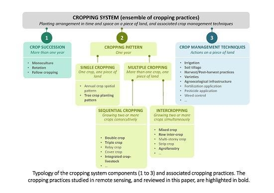
2. Typology of the Cropping Practices

Some agronomic terms do not have an international and unique definition. Therefore, certain technical agronomic-related vocabulary is sometimes misused in remote sensing publications. To ensure clarity, we wanted to start this paper by defining the agronomic terms used hereafter, referring to the most common definitions, and respecting the agronomic conventions as closely as possible.
In this paper, “cropping practices” describes the elements of a cropping system. A cropping system refers to the crop type, sequence, and arrangement, and to the management techniques used on a particular field over a period of years [7,8]. The cropping system can be described by the following three components, each of them being defined by a set of cropping practices (Figure 1): (1) a temporal component describing the sequence of crops or fallows for consecutive years, referred hereafter as “crop succession” (number 1 in Figure 1); (2) a component describing the yearly sequence and spatial arrangement of crops and fallows in a particular land area, referred hereafter as “cropping pattern” (number 2 in Figure 1); and (3) a crop management component that corresponds to the techniques, such as irrigation or soil tillage, implemented on a piece of land (number 3 in Figure 1).
In the subsequent sections, only the cropping practices that were studied in remote sensing are presented, and highlighted in bold in Figure 1. Some pastoral practices related to their production management are also included. Notably, the list of the studies reviewed in this paper is certainly incomplete as we were not aiming to be exhaustive but to report the representative results.

3. Crop Succession

The term “crop succession” refers to the sequence of crops or fallows in consecutive years. Thus, monoculture, crop rotation, and fallowing, which is the practice of sequences of crop years and fallow years, are different types of crop succession. Differentiating between these three types of crop succession is important because they have different impacts on food production and natural resources management.

3.1. Monocropping and Crop Rotation

Crop rotation is a useful technique for soil management, controlling pathogens, pests, and weeds, for removing excess nutrients in the soil, and correcting nutrient deficiencies of soils. While monocropping is generally practiced in intensive agricultural farms, where large amounts of resources are available to improve the production process, crop rotation is a necessity for low-input farms. Crop rotation is a reasoned process where choosing the crop species for succession is not random, but follows recommended patterns [9]. For example, a nitrogen depleting crop should be followed by a nitrogen-fixing crop, and a low residue crop by a high biomass cover crop [10].
Monocropping and crop rotation can be directly assessed with annual crop type maps, by extracting the sequence of crop types at the field scale for more than two years. In the Midwestern United States, Stern et al. [11] analyzed 10 years of annual remote sensing crop classifications from the National Agricultural Statistics Service of the United States Department of Agriculture (USDA), to define the corn-soybean rotation dynamic in relation to the market prices. In the Kiev region, Ukraine, highly accurate crop type maps were produced using a combination of neural networks applied to optical and radar image time series acquired during the period of 2013 to 2015 [12,13]. A crop rotation violation map for the Bilotserkivskiy district was then produced, showing fields where winter wheat, winter rapeseed, sunflower, and maize were grown in the same fields for at least two or three years, contrary to the agricultural policy in place. Sahajpal et al. [14] developed the Representative Crop Rotations Using Edit Distance (RECRUIT) algorithm that selects representative crop rotations by combining and analyzing maps of the major agricultural crops traded on the U.S. commodity markets, produced annually from remote sensing data by the USDA.
However, Mueller-Warran et al. [15] outlined that although converting multi-year land-use data into crop rotation history is relatively simple in theory, the presence of classification errors can severely compromise the results. Given this fact, they proposed using a matrix of logically forbidden or extremely unlikely year-to-year land use transitions to detect classification errors. Likewise, the use of a priori knowledge of the local rotation practices could be a research area for improving crop type identification by constraining classification models.

3.2. Crop-Fallow Rotation/Fallowing

Hereafter, fallow refers to arable land that is set aside for a period of time ranging from one to five or more years before being used again for cultivation. Fallow aims to regenerate natural resources, such as soil and water, after exploitation, and represents about 28% (4.4 million km2) of the global cropped areas [16]. Updated knowledge about the extent, frequency, and duration of fallow land provides baseline information for policy making and resource planning, such as cropland intensification vs. cropland area expansion [17] and allocation of scarce water resources for on-farm use [18].
Existing land use and land cover studies commonly merge the cropped and fallowed fields in a common class [19]. Due to the wide range of existing fallow practices, mapping of these areas is a difficult task [16]. A fallowed field may be confused with cropped fields due to climatic and soil conditions [20], cropping techniques [19], crop failure [16], or may be confused with surrounding ecosystems due to its natural regeneration.
Despite these difficulties, examples of methods for fallow characterization using remote sensing data exist in the literature. This characterization is generally performed in three steps: (1) cropland mapping, (2) annual/seasonal fallow mapping inside the cropland mask using satellite time series, and (3) multi-annual analysis of the fallow maps to determine the fallowing frequency, also known as the fallow age. Xie et al. [21] showed that masking the non-agricultural areas blended with agricultural fields was a critical pre-processing step for distinguishing active crops and fallow lands. In Niger, Tong et al. [19] developed a classification approach based on the different phenological characteristics of the vegetation, including Normalized Difference Vegetation Index (NDVI), amplitude, and rate of decrease rate, as monitored by a MODerate-resolution Imaging Spectroradiometer (MODIS) 250 m resolution data. They showed that fallowed fields generally have a higher NDVI and a more rapid decrease than unmanured cropped fields (Figure 2). In the Central Valley of California, Melton et al. [18] tracked land fallowing using a NDVI time series based on Landsat data completed with MODIS data, and monthly ground data collections. They used a decision-tree algorithm to evaluate the information about a set of phenological metrics extracted from the NDVI time series, and the land-use changes relative to previous years, to assign each field to a land-use class. The classification accuracy was above 85%, and the authors noticed that the primary sources of error were confusion between young fallows and recently planted perennial crop fields, and errors associated with field boundaries or partially planted fields. To overcome the constraints of ground data collection, for the same area, Wallace et al. [22] developed and applied a Fallow-land Algorithm based on Neighborhood and Temporal Anomalies (FANTA) that routinely mapped cropland status (cropped or fallowed) with user and producer accuracies over 75%. The FANTA algorithm compares the current greenness of a cultivated pixel to its historical greenness and to the greenness of all cultivated pixels within a defined spatial neighborhood. Good results were obtained applying FANTA to annual row crops, but the study encountered the same difficulty as Melton et al. [18] for perennial crops that have a much more diverse growth cycle.
The examples above show that fallows and the surrounding crops (especially perennial crops) or natural vegetation are commonly confused, and these confusions are spatially heterogeneous due to varying climatic and soil conditions, and cropping practices. As a result, methods to accurately monitor active, fallowed, and abandoned cropland are still lacking for many regions in the world [20]. Closely monitoring the vegetation development for the same piece of land over several years with regular satellite imagery acquisition and processing is one area to continue to explore.

4. Cropping Pattern

Cropping pattern is defined here as the yearly sequence and spatial arrangement of crops, or of crops and pasture, on a given piece of land. Multiple cropping is when more than one crop is involved, as opposed to single cropping.

4.1. Single Cropping

For single cropping, the cropping pattern refers to the spatial arrangement of the crops. The vast majority of the remote sensing studies address the spatial patterns of tree crops, such as orchards and vineyards. Few studies have reported on annual crop row orientation [23].

Tree Crop Planting Pattern

Tree crops represent a significant part of agricultural landscapes, and their specific cropping practices mean they must be mapped separately from annual crops. The knowledge of their presence and associated cropping practices contributes both to landscape ecology and economical surveys. Some tree crops, such as nut groves and vineyards, are eligible for support payments from the European Common Agricultural Policy for specific plot sizes and tree planting densities [24]. Remote sensing has thus been developed as a tool for subsidies control, for instance, with the first goal being to map the areas of permanent crops.
This subject appears to be a challenge for optical remote sensing because of the considerable spectral and spatial heterogeneity and variability in the object of study, such as for plant layout, density, and structure. As comprehensively described by Aksoy et al. [25], although some spectral features analysis succeeded in discriminating structured plots [26], automatic orchards and vineyards mapping methods have mostly been developed based on the textural approach, using various structural indicators such as indices derived from the co-occurrence matrix [27,28], autocorrelograms [29,30], Markov random fields [31], and frequential analysis [32,33,34,35]. Peña-Barragan et al. [36] showed that multispectral imagery is suitable to discriminate cover crops from olive trees and to estimate olive tree surface with good accuracy (92%). Panda et al. [37] reviewed several techniques used in fruit and nut crop management and described the methods used to differentiate orchards from other land uses, and how GIS and models can then be applied for analyses. No accurate discrimination of tree crop types has been achieved without a significant input of field knowledge.
Most remote sensing studies that addressed tree crop planting patterns focused on vineyards, and less on olive and nut groves. Even if some studies showed the feasibility of separating different cropping structures, such as simple row vs. pergola (continuous trelliswork) in large vineyards using decametric resolution images [38] with ASTER (Advanced Spaceborne Thermal Emission and Reflection Radiometer) data at a spatial resolution of 15 m, most authors highlighted the need for high spatial resolution images, with metric and sub-metric resolution, to detect intra-field cropping structure. The best imagery was acquired from Unmanned Aerial Vehicles (UAV) or UtraLight Aircrafts (ULA). Delenne et al. [39] showed that simple local Fourier analysis and co-occurrence matrix-based indices, applied to very high spatial resolution images acquired with an ULA, detected vineyards and characterized intra-field cropping patterns (simple row vs. pergola), and rows and inter-row orientation and scale. Along the same lines, Amoruso et al. [29] used a variogram-based texture algorithm to discriminate olive groves from forest and other vegetation land use classes. More generally, Yalniz and Aksoy [40] used wavelet analysis of image texture to discriminate between tree crops of various regularity, in terms of periodicity, orientation, and scale. Lefebvre et al. [41] also proposed wavelet decomposition for a textural pattern analysis, improving vineyard detection and cropping pattern (row orientation) characterization. However, some researchers consider Light Detection And Ranging (LiDAR) technologies as the more relevant tool to map tree crowns and derive structural information, and an abundance of three dimensional (3D) studies can be found in the literature for tree crop structure characterization based on LiDAR [42].
Several studies focused on tree crown status, using images at spatial resolutions smaller than one meter, after manual delineation of the tree [43]. Others developed methods and algorithms, such as local maximum filtering and valley-following, to automatically delineate tree crowns [44,45,46], where the tree detection ability is closely linked to the often sub-meter image spatial resolution. Most of these algorithms were developed to detect trees in forests, but obtain good results for fruit groves that display a simpler structure. Torres et al. [47] developed software (CLUstering Assessment or CLUAS) to provide some quantitative agronomical parameters and environmental indicators in olive groves, such as the number of olive trees, the size of each tree, the fraction of soil covered by trees, or the potential productivity based on density calculations. However, hyperspectral and/or UAV technologies are needed for good accuracy in tree detection [48]. Stereo imagery at very high spatial resolution, which obtains surface and elevation models, is also promising but only in situations with good contrast between the tree crown and its immediate environment to allow correct matching of the stereo pairs.

4.2. Multiple Cropping

4.2.1. Sequential Cropping

Sequential cropping consists of harvesting more than one crop sequentially during the same growing season. In areas with sufficient rainfall and a long frost-free period, one, two, or even three harvests are possible per year [49]. The main reason for adopting sequential cropping systems is economic since it creates a rapid increase in the land productivity. Nonetheless, sequential cropping can also be related to the adoption of ecological cropping practices. For example, the second crop is often sown both to benefit from the end of the rainy season and to enable the adoption of no-tillage practices [50,51]. By doing so, the soil quality is improved by limiting the loss of chemical products and organic matter via erosion, and by retaining water for a longer period, which allow farmers to achieve better yields [50,51]. Sequential cropping may also help fight against crop diseases, as was the case with the Asiatic rust soybean disease, whose expansion in the Southern Amazon was aided by the soy monoculture. Finally, since double cropping increases crop production in existing agricultural areas, it limits land use changes such as tropical deforestation driven by agricultural expansion [52,53,54].
Remote sensing-based characterization of sequential multiple cropping relies on the use of high temporal resolution time series to ensure accurate monitoring of the phenological cycles [49,55] and capture the seasonal variability and crop calendars of sequential cropping systems (Figure 3). Good expert knowledge of the local to regional agricultural practices is thus required. Coarse spatial-resolution satellite imagery with high revisiting frequencies, such as NOAA-AVHRR [56] (National Oceanic and Atmospheric Administration-Advanced Very High-Resolution Radiometer) or SPOT-VGT [57,58] (Satellite Pour l’Observation de la Terre-Vegetation) are usually preferred, but MODIS data has long received more attention for this type of application due to its daily acquisitions and 16-day composites of vegetation indices (Enhanced Vegetation Index (EVI) or NDVI) with a 250 m spatial resolution. MODIS data have been successfully used to map sequential multiple cropping in various agricultural areas with relatively large fields, especially in the United States, China, and Brazil. In the U.S. Great Plains (Kansas), Wardlow et al. [55] assessed the potential of NDVI and EVI time series to separate crop types and cropping systems, which were subsequently mapped [59]. In Northern and Central China, Mingwei et al. [49] and Qiu et al. [60] mapped single (cotton or maize) and double cropping systems (winter wheat-cotton, winter wheat-maize, and winter wheat-rice) based on Fourier and wavelet analysis, respectively. In the Brazilian Amazon, studies conducted at the local level explored the potential of MODIS vegetation index time series to discriminate single- and double-cropping systems (soybean and soybean-maize or soybean-cotton) [61,62]. These studies were then upscaled to regional-scale maps of these systems over the entire state of Mato Grosso [63,64,65].
In these studies, Vegetation Index (VI) time series are generally pre-processed to limit misclassification due to noisy data. Although the MODIS VI data are made of composite values, low noise VI values may remain in tropical areas with an intense rainy season. To correct these values, various smoothing algorithms can be used [66], as well as wavelet analysis [62]. Most of the studies then train supervised classifications with reference data, usually in the form of ground observations [49,63,64]. Unsupervised classification approaches are somewhat less common but have achieved good results when adopting hyperclustering methods [17,59,67]. Clustering approaches do not require ground data, which are time- and resource-consuming to collect, especially when data must be gathered twice during the growing season over large areas. However, labeling the final classes relies on adequate knowledge of the local to regional agricultural practices, which allows relating the different phenological cycles to the crop calendars to ultimately identify crop types.
The main issue for classification is the high intra-class variability in the sequential cropping systems. The same cropping system can be characterized by different crop calendars due to regional climatic differences [52], specific climatic events in some given years (e.g., a longer dry season that caused delayed sowing), and logistical issues, such as the sowing period lasting a few months in very large farms. To address this issue, different approaches are implemented to classify the satellite time series. Time series may be processed to extract features, such as in Morton et al. [68] where 36 metrics from MODIS VI time series were computed, including NDVI and EVI minimum, maximum, mean, median, amplitude, and standard deviation for annual wet and dry seasons, which were subsequently classified. Arvor et al. [63] searched for the best dates of the time series that maximized the separability distance between the EVI profiles of six classes of cropping systems. Innovative techniques, such as Fourier analysis [49] or wavelet analysis [60], provide a new representation of image time series, allowing for a finer analysis of vegetation phenology. Nonetheless, these techniques are based on a reduction dimension which implies a loss of information. To address this issue, new techniques, such as Dynamic Time Warping approaches with temporal weights, were successfully tested to classify land cover classes including single and double cropping systems, based on shape matching of MODIS EVI time series [69]. Bailly et al. [70] implemented a Dense Bag-of-Temporal-SIFT-Words approach, which involves representing vegetation index time series in sequences of local features, such as peaks and constant growth. These features were then used to build histograms of patterns corresponding to new time series representations to be classified by traditional classifiers, such as support vector machine (SVM).
Complementary studies evaluated the potential of Synthetic Aperture Radar (SAR) imagery for monitoring multiple cropping systems. For example, some studies demonstrated the potential of ENVISAT ASAR (Advanced Synthetic Aperture Radar) time series to detect single-, double-, and triple-cropped rice areas in the Mekong Delta River [71,72]. Bouvet et al. [71] showed that the detection of a high backscatter increase at the beginning of the growing cycle allowed for the production of rice maps early in the season. However, these studies were limited by the poor acquisition frequency of the available SAR data. They used incidence angle normalization methods and/or temporal averaging to combine acquisitions from multiple tracks and years. This limitation is now outdated due to the launched SAR Sentinel-1 sensor that provides dense time series with a temporally-consistent incidence angle.

4.2.2. Intercropping/Agroforestry

Few remote sensing studies address intercropping. This can be explained by the infra-metric scale of the intra-field variability of mixed crop fields. Only agroforestry systems can be considered as an exception, and are detailed hereafter.
Agroforestry is the practice of growing crops and trees, and sometimes keeping animals, together. This is a multifunctional land-use system and technology that provides a wide range of economic, sociocultural, and environmental benefits [73,74]. The ecologically-based dynamic integration of trees on farms and in the agricultural landscape diversifies and sustains production for land users at all levels, enhancing food supply, income, health, and environmental sustainability, even in the most industrialized nations [75]. Among these benefits, agroforestry supports food production by enhancing fertility [76,77], controlling soil erosion [78,79], improving water quality [80,81]), and by sequestering substantial quantities of carbon [82,83].
Agroforestry is a challenging cropping system to monitor using remote sensing because of its spatial heterogeneity and complexity. Agroforestry cropping patterns can range from the regular intercropping of two or more types of crops, whose rows vary from one to five meters in width, to a totally random distribution of dozens of different tree species and sizes in a closed canopy. Due to this wide range of heterogeneity, discriminating different agroforestry systems based only on their spectral signature is almost impossible. Some authors classified agroforestry systems using only Landsat TM spectral response, but only for scenarios where a single kind of tree is in focus: rubber trees cropped as a monoculture on one side and rubber associated with other species as the agroforestry crop on the other side [84], or poplar-based agroforestry systems being the only intercropping practice in the studied area [85]. Lelong et al. [86] introduced a Canopy Closure Index derived from the Quickbird multispectral signature, helping to describe the structure and complexity of coconut-based agroforestry systems in Melanesia using in-field observations as keys for the interpretation. In general, the detection of the individual pattern elements, such as trees, rows, and stripes, is needed to characterize the agroforestry cropping pattern, and even to detect the use of agroforestry itself. This implies the images used must provide at least 1 m spatial resolution, as is available from Ikonos, Geoeye, Quickbird, Worldview, or Pleiades. As an example, Lelong and Thong-Chane [28] showed that integrating Haralick textural indices associated with radiometric profiles in the pixel-based classifications of Ikonos images allowed discriminating between tropical tree monocrops (mango, eucalyptus), intercrops (banana and coffee), and crops associated with shading trees (coffee under albizias) in Uganda. Lelong et al. [87] showed that an object-based approach for WorldView2 image classification, based on multiscale segmentations and the joint use of textural and spectral indices, results in good discrimination of several types of cocoa-based agroforestry systems in Cameroon, based on their planting structure and heterogeneity. Karlson et al. [88] also largely insisted on the importance of the object-based approach and the high spatial resolution in agroforestry system detection and classification, even in scattered canopies like West African parklands. Gomez et al. [89] based their processing of Quickbird imagery on a preliminary detection of tree crowns, and added indicators, such as tree crown size and heterogeneity of the canopy, to textural and spectral indices to map coffee-based agroforestry systems in New Caledonia. In many cases, visual image interpretation remains the most accurate method to discriminate and characterize agroforestry system cropping patterns, such as for complex coffee, citrus, and clove food crop associations in Bali [4].

5. Cropping Techniques

Crop management techniques are the ensemble of techniques used to grow a given crop on a given land, from the soil preparation to the post-harvest practices, including application of inputs (fertilizers, irrigation, pesticides and herbicides), crop variety selection, harvest mode, and implementation of agro-ecological structure associated with the fields. Not all techniques can be remotely sensed, but some can be easily identified from space. Hereafter, we chose only to present the crop management techniques that were largely represented in the remote sensing literature. However, we are aware that many other practices have been investigated, such as, for example, cover crop adoption [90] or plastic-mulching in China [91]. Fertilization is a specific case, as many studies exist on the use of remote sensing for estimating the status of a wide range of crops in terms of nitrogen, phosphorus, or potassium content, but to our knowledge, none of them focused on mapping the existence or absence of fertilization. Consequently, this crop management technique is not addressed in this paper.

5.1. Irrigation

Among all crop management techniques, irrigation is of prime importance for increasing crop productivity. Since the 1970s, agricultural production has doubled within an area that has only increased by 12%, and a part of this gain can be attributed to an increase in irrigation [92]. According to Bastiaanssen et al. [93], around 50% of the world food is produced under irrigation or drained soils, making agricultural production responsible for about 80% of global water consumption. Expansion of irrigated agriculture is thus one of the driving forces for the rising global demand for water [94]. Due to growth in population and food demand, irrigated areas are expected to almost double by 2050 in a context of climate change and decreasing water availability [95], while causing significant environmental changes. Consequently, cropland products should discriminate between crop watering methods (rainfed vs. irrigated areas) to monitor crop water use and analyze food security scenarios [96].
Remote sensing can provide valuable information related to irrigation that can be applied to water management planning and evaluation, including water use, performance diagnosis, strategic planning, and impact assessment [97]. We focus here on the use of remote sensing for identifying and mapping irrigated areas. We considered irrigated land as areas, from smallholder to intensive farming, artificially receiving full or partial supplemental irrigation to compensate for the insufficient precipitation during the growing season [92].
Although many remote sensing studies and applications exist for mapping cropland or crop type at different scales, fewer studies are available for the identification and mapping of irrigated cropland [92]. Due to its dynamic characteristics, agriculture is known as a difficult land cover type to map, and is more challenging for high temporal image acquisitions. The same observation can be made for the mapping of the subclass “irrigated lands”, with the addition of different irrigation techniques such as flood, drip, or spray irrigation, and the spatio-temporal scheduling of irrigation. Studies addressing the topic of irrigation mapping from remote sensing are based on the use of images from different sensors (optical, radar, or both) and on different classification methods depending on the scale of the study (local, regional, continental or global). The review of Ozdogan et al. [92] analyzed the requirements for monitoring irrigated areas in terms of spatial, spectral, and temporal information, and report on the existing approaches for each scale.
The local scale is the most documented, as methods can be tested in a more controlled environment with less variability in irrigation practices, with using a considerable amount of ground data and expertise, and uses costly high or very high-resolution imagery without a necessary operational objective. Historically, the first methods principally used photointerpretation, with Landsat 1 imagery alone [98,99], or combined with field boundary information [100]. These methods are maybe the most accurate, but are the least efficient in terms of time and human resources. Consequently, automated classification approaches were developed, including unsupervised classification [101], single or multi-stage supervised classification [102], decision tree [103], and supervised learning models such as Random Forest or Support Vector Machines [104,105]. Furthermore, Li et al. [106] showed that the object-based image analysis (OBIA) approach applied to Landsat, which allowed the use of information about the geometry and topology of the fields, was useful for discriminating irrigated fields. All these methods exploited the spectral difference, in terms of reflectance, spectral indices, or other derived features, between irrigated areas and other land cover types. Among the spectral indices, the NDVI was commonly used because of its differential spectral response in presence of either irrigated or rainfed crops. The analysis of multiple satellite acquisitions over a growing season was shown to be more efficient, as it reflects the differences in phenological evolution between crops [107]. However, when a peak was observed within a known given small time period in an irrigation season, one image acquired at the right time may suffice to identify irrigated areas [92]. In tropical regions where optical imagery is affected by cloud coverage, studies are based on the use of SAR data. For example, Choudhury et al. [108] used Radarsat-1 time series to discriminate rice crop water regimes (shallow, intermediate and deep water rice) with very high accuracy (98.8%) based on the sensitivity of SAR backscatter to crop geometry and water combined with a knowledge-based classifier.
At the regional scale, methods generally rely on the use of coarse spatial resolution data, such as MODIS, AVHRR, or SPOT-VGT for their high temporal resolution and their ability to monitor the crop phenology through time and over large areas [109,110,111,112,113]. Decametric resolution images, like Landsat images, can also be used alone or to complement the previously cited data [114]. To characterize irrigated land using this data, methods are mostly based on the analysis of spectral indices time series, and aim to identify the specific temporal dynamics of irrigated crops, as performed by Xiao et al. [113] on paddy rice with the succession of flooding, transplanting, growing, and fallow periods determined through the analysis of NDVI, EVI, and especially generally Land Surface Water Index (LSWI) temporal profiles. Another study on rice relied on the automatic detection of vegetation peaks along the growing season with SPOT-VGT NDVI time series, allowing the discrimination between rainfed (one peak) and irrigated (multiple peaks) rice [115]. Other authors used unsupervised classification [110] or decision tree methods [114] to map irrigated crops from MODIS time series. In Biggs et al. [110], the final classification even included the discrimination between different irrigation techniques based on a 45-day gap observed between greening of areas irrigated by surface water and groundwater. Dheeravath et al. [111] also introduced an OBIA approach by segmenting a three-year MODIS reflectance time series acquired at eight-day intervals, prior to the classification step performed using spectral matching techniques. Even if most of the studies use vegetation indices time series, Thenkabail et al. [116] showed, on MODIS data, that some original spectral bands, especially band 5 (1240 nm) provided a good degree of discrimination between rainfed and irrigated areas.
At the global scale, the first products such as the USGS (United States Geological Survey) Global Land Cover Map [117] developed from 1-km AVHRR data did not specifically focus on irrigated areas, thus leading to low accuracy for the four irrigated classes of the product. Similar to this method, the GlobCover product, derived from unsupervised clustering of 300-m MERIS (MEdium Resolution Imaging Spectrometer) data and expert labeling rules, provided irrigation classes among other land cover types [118]. Then, Thenkabail et al. [119] specifically mapped irrigated areas by analyzing AVHRR time series using spectral matching techniques, such as spectral similarity. A dedicated product, the Global Irrigated Area Map (GIAM), was produced by using multi-source data (AVHRR, SPOT-VGT, JERS-1 SAR, rainfall, temperature, and elevation) in an approach applying segmentation, unsupervised classification, spectral matching, decision tree, and spatial modeling steps [120].
Identifying small or fragmented irrigated areas on a large scale remains complicated due to the spatial resolution of the imagery available for operational applications (i.e., free data with high repeatability over large areas cannot always be obtained) [110,121]. In these areas, the use of metric or sub-metric spatial resolution data coupled with an OBIA approach can better identify cultivated fields using segmentation. Velpuri et al. [121] studied the influence of spatial resolution in irrigated area mapping and estimation. Due to their ability to detect small and fragmented irrigated areas, high spatial resolution imagery (Landsat 30 m in this study) provided more precise location and area estimation of irrigated areas (84%) compared to MODIS (250 m: 79%; 500 m: 77%) or AVHHR (1 km: 63%). The recent availability of the Sentinel-2 mission, providing high spatial (10–60 m) and temporal (five days) resolution imagery may offer improvements for these types of agricultural landscapes. Nevertheless, even if less efficient for fragmented croplands, methods exist for performing area correction on low spatial resolution products with the use of high spatial resolution reference data [110].
When using optical imagery, frequent cloud cover in tropical areas negatively impacts these methods, so methods based on the use of SAR data are thus preferred in these areas. The identification of irrigated areas is also easier to complete over arid or semi-arid regions. In these regions, almost all vegetative growth is linked to irrigation [107] and only a few classes have to be distinguished, whereas in humid areas, natural wetlands can be confused with irrigated areas [92].

5.2. Soil Tillage

Tillage, defined as the set of soil operations performed for various reasons including seedbed preparation, weed control, nutrient incorporation, and water management, is a key aspect of cropping systems. Tillage modifies the soil cover, water content, temperature, aeration, and aggregation, affecting soil organic carbon and nutrients, soil susceptibility to erosion, and soil organisms [122]. In particular, the role of crop residue cover in the protection of agricultural soils against water or wind erosion is very important. In the United States, estimates of soil loss due to different tillage practices ranged from 328 kg/ha/y to 8619 kg/ha/y [123]. In the Pampas region of Argentina, differences of up to 3 Mg/ha of soil organic carbon (C) were observed due to tillage practices [124]. Tillage practices can be coarsely classified as conservation or conventional, based on the amount of plant litter remaining on the soil surface. Conservation tillage generally involves few interventions, and is also referred as no-tillage (i.e., direct sowing) or reduced tillage (i.e., vertical tillage) practices. In general, conservation tillage maintains more than 30% of the residue cover [125]. Conversely, conventional tillage generates considerable soil displacement as the soil is turned over and furrows are cut by plough implements. As initial soil aggregates are coarse, conventional tillage requires several interventions before sowing.
Remote sensing approaches are based on the assessment of the two features that are strongly modified by tillage systems: residue cover and surface roughness. Many studies have reported on the qualitative and quantitative estimation of residue cover with optical multi or hyperspectral sensors (see review by Zheng et al. [126]). Optical remote sensing exploits the spectral differences between crop residues and soil using the shortwave infrared region of the electromagnetic spectrum and, particularly, with an absorption feature from cellulose and lignin at 2100 nm [127]. For example, South et al. [128] tested five supervised classification methods to map no-till and conventional tillage using a single Landsat 7 ETM scene. They found that the spectral angle methods outperformed the conventional methods, with an overall accuracy above 96% and a Kappa above 0.92. Similarly, Sudheer et al. [129] found acceptable results, with overall accuracies ranging from 66% to 91%, using artificial neural networks and single Landsat 5 TM scenes. However, Bricklemyer et al. [130] failed to detect tilled fields using a single Landsat scene using regression and classification trees, suggesting that discrimination ability is time dependent. Indeed, Watts et al. [131] significantly improved tillage classification accuracy by increasing the number of Landsat scenes fed to a random forest classifier. The results of Watts et al. (2011), highlighted the inadequacy of one Landsat scene for capturing the agricultural dynamics imprinted by several farmers’ individual decisions about crop planting and management.
Quantitative approaches mainly rely on linear regression with spectral indices designed to maximize the crop residue signal and the fractional cover of crop residue [126]. Tillage indices vary according to the sensor used, with the most frequently used being the Cellulose Absorption Index (CAI), requiring hyperspectral sensors such as AVIRIS (Airborne Visible/Infrared Imaging Spectrometer) or Hyperion [132], and the Normalized Difference Tillage Index (NDTI), which can be obtained from Landsat or MODIS sensors [133]. Other indices include the Lignin Cellulose Absorption [132] and the Shortwave Infrared Normalized Difference Residue [134], both calculated from ASTER, and crop specific and/or soil adjusted indices such as the Crop Residue Index Multiband [135], the Modified Soil Adjusted Corn Residue Index [136], and the Shortwave Angle Slope Index [137]. In general, these indices showed promising results with a Root Mean Square Error (RMSE) ranging from 8.2% for CAI to 13.6–20.9% for NDTI in 2008 and 2010, respectively [138]. However, the results depended on environmental conditions such as soil moisture or residue water content. Alternative quantitative approaches have been explored using constrained linear spectral mixture analysis of Hyperion data [136]. These authors reported a R2 of 0.73 and a RMSE of 8.7% for percent cover of crop residue and a R2 of 0.68 and RMSE of 10.3% for soil percent cover. Similarly, Pacheco and McNairn [139] reported a RMSE of 17.3% and 20.7% for percent crop residue cover when using spectral unmixing analysis of Landsat 5 TM and SPOT 4/5 images, respectively.
Roughness-based approaches rely on SAR data. Soil roughness was related to the application of different tillage practices showing RMSE values of height between 0.5 and 0.7 cm for smooth and no-till surfaces, and 3.2 cm for moldboard plow implements, with intermediate values for chisel plow (2.3 cm) and disks (1.8 cm) [140]. SAR systems can respond to soil surface roughness [141,142,143], since their wavelengths are similar in magnitude compared to soil height variations. Nevertheless, few studies related backscatter signal to tillage practice mapping. Pacheco et al. [144] evaluated the use of single and dual-pol (HH and HV) X band SAR (TerraSAR-X) to discriminate between moldboard ploughed and untilled fields. At C band, McNairn et al. [145] showed differences between the backscatter signal of two different tillage implements, chisel and moldboard, and no-till, associated with the differences in roughness. C and L band backscatter were also positively associated to residue cover [146], which complicates the ability to separate conventional (low residue) and no-till (high residue) practices using SAR. Hadria et al. [147] considered the combined use of SAR and optical sensors. They found a clear separability between tilled fields and no-tillage fields using the SAR C band (Envisat ASAR VV polarization), whereas near-infrared reflectance showed a clear separability between different practices (plowing and harrowing). SAR-optical complementarity allowed for better discrimination of these three groups. Turner et al. [148] investigated the feasibility of using airborne LiDAR observations to track changes in surface roughness due to farming activities. LiDAR- and field-derived heights Root Mean Square estimates were shown to be highly correlated (R2 > 0.68 and up to 0.88) and accurate (RMSE < 0.81 cm, bias < 0.48 cm), suggesting that developing detection methods for the estimation of tillage changes may be possible.
Still, several issues challenge regional to global scale remote sensing of soil tillage [126]. First, the combined effect of the broad differences in the timing of tillage operations and the relatively low frequency of cloud-free acquisitions of the satellite sensors used is often an issue. Second, confounding effects are present with soil and crop residue moisture content, soil spatial variation, and green vegetation spatio-temporal variability. Third, the definition of the spatial and temporal extent for the application of empirical models is challenging. Fortunately, some of these constraints can be reduced due to the recent availability of Sentinel-1 and 2 images together with Landsat 8, and the potential capability of synthetizing Landsat images at the MODIS temporal resolution using the Spatial and Temporal Adaptive Reflectance Fusion Model (STARFM) [149]. Zheng et al. [150] developed a multitemporal approach to minimize the confounding effects of green vegetation. Using this approach, the authors reported a R2 of 0.89 between the minNDTI (the minimum NDTI from a NDTI time series) and crop residue cover in central Indiana, U.S. Moreover, the increasing availability of multiband or multifrequency SAR data allows independent assessment of soil surface moisture, which could then be used to interpret optically-based tillage mapping. Specifically for SAR, Quad-Pol configurations help separate roughness from other factors, such as soil moisture [151]. With the exception of Radarsat-2, current (like Sentinel-1) and future radar missions (like Radarsat-constellation) do not consider Quad-Pol, or their configuration is infrequent (e.g., ALOS-2 and TerraSAR-X). In addition, as soil roughness can change quickly (e.g., because of precipitation), the timing of SAR image acquisitions is not always optimal.

5.3. Harvest

5.3.1. Detection of Harvested Area

The detection of harvested crops that are cultivated year round or over a long time period (several months) is a key piece of information for the transformation and commercial sectors. For example, in smallholder sugarcane production regions, updated information on the status of the cane fields or blocks for the whole area serviced by the mill may help to better estimate the effective yield, and better assess the standing cane areas to be harvested, thus optimizing the cutter deployment and transport operations. Only examples on sugarcane harvest detection were found in the remote sensing literature and are summarized hereafter.
In 2007, using a SPOT image time series and a sugarcane crop mask, Lebourgeois et al. [152] mapped the sugarcane harvest on Reunion Island using the ISODATA algorithm with an overall accuracy of 97.5%. Aguiar et al. [153] used fraction images derived from linear mixing models in a decision-tree procedure to identify sugarcane harvest for the entire São Paulo State, aligning by 97.7% with the State Environmental Secretary data. However, the authors had difficulties in defining suitable endmembers. Despite the good results with optical images, cloudy conditions are a limitation. The interval between two cloud-free images is sometimes longer than two months, which complicates the discrimination between a standing crop and the regrowth in a field harvested at the beginning of the harvest campaign. El Hajj et al. [154] proposed an approach that integrates satellite time series analysis, crop growth modeling, and expert knowledge, to address this uncertainty. Alternatively, Baghdadi et al. [155,156] used SAR data exploiting day and night measurements that are acquired regardless of meteorological conditions. Using radar time series acquired over sugarcane fields in Reunion Island with different wavelengths (X-, C-, and L-bands), they showed that even if the radar signal increased with crop height until reaching a threshold, the plant and soil water content modify this relationship. With ASAR images, they observed a decrease in radar signal of the same magnitude after a harvest or after the sugarcane plants dried [155]. Using TerraSAR data, they showed that the cut was easily detectable for data acquired less than two or three months after the harvest, unless strong rain events affected the radar signal [156].

5.3.2. Harvest and Post-Harvest Practices

In this section, harvest and post-harvest practices involve plant biomass and crop residue burning. When the plant biomass is not the crop end product, as for sugarcane, the harvest can be performed with preliminary crop burning (burn harvest), or mechanically without crop burning (green harvest). The burning practice aims to facilitate manual harvesting through the removal of leaves and dangerous animals, and mechanical harvesting by reducing the quantity of biomass to transport to the sugar factory. With respect to crop residue management, open straw burning is a widespread practice for cereals in tropical regions, in particular when the turn-around time between two cereal crops is very short. Burning of crop residues improves tillage efficiency and reduces the need for herbicides and pesticides to control diseases, weeds, and pests. However, in both cases, standing biomass or crop residues, the products of burning are emitted into the atmosphere affecting both the local air quality and the global climate, contributing to the emission of harmful air pollutants [157], and reducing carbon sequestration. The practice also creates a risk of fires spreading out of control. For these reasons, governments have increasingly restricted its use. Remote sensing is an effective way to assess the dynamic of this practice.
A first approach involves using global fire products. In Brazil, Tsao et al. [158] showed that these products underestimate burned areas, due to the small size of the individual sugar-cane fires relative to the 500 m resolution of the MODIS product. Another approach is the use of time series of decametric optical images that are better adapted for distinguishing burn harvest and green harvest at the field scale, due to the strong contrast between dark burnt fields, where bare soil is dominant after harvest, and bright green harvest fields, where a layer of dry leaves (straw) covers the ground after harvest. The spectral contrast remains high for several days or even weeks after harvest [159] (Figure 4), especially in the shortwave infrared domain, making this band a good candidate for harvest mode discrimination [160]. However, Goltz et al. [161] showed that the harvest mode classifications were sensitive to the soil type, and that in regions with different soil types, lighter soils can generate uncertainty between the types of sugarcane harvest.
Since 2006, based on these contrasted spectral properties of the surfaces, the National Institute for Space Research (INPE) has monitored the sugarcane harvesting practices in São Paulo State and generates monthly and annual maps of the sugarcane harvested areas with and without the pre-harvest burning. These maps are produced by visually interpreting one decametric image coverage per month over the harvest season, and using a sugarcane crop mask [162]. Although visual interpretation can be effective for sugarcane harvest characterization, it is a laborious task and impractical for very large areas or throughout a long harvest season. Mello et al. [159] proposed an alternative automated classification procedure, based on the Spectral-Temporal Analysis by Response Surface (STARS) that synthesizes the full information content of a multitemporal/multispectral remote sensing image dataset, to represent the spectral variation of features on the earth’s surface over time. Applied to sugarcane, they obtained high Kappa values (>0.9 in many cases) for harvest detection and harvest mode mapping. In conclusion, harvest date and mode detection requires the use of a time series, mainly optical, since radar remains ambiguous with soil and plant water status.
For crop residue management in Taiwan, Liu et al. [163] used FORMOSAT-2 satellite images and ground-truth data to conduct a supervised classification of the visible bands only, and calculated the extent of the straw burning areas. The study determined that more than 10% of the total paddy area was burnt during the 2008–2009 period, which is in line with the current actual situation. On this pro rata basis, Chang et al. [157] calculated the air pollutant emissions due to the straw burning practices in the region. In conclusion, the detection of open straw burning is based on the color of the land surface, equivalent to the detection of burn harvest. Other surface conditions may complicate the classifications, but globally, the classifications achieve good results.

5.3.3. Grazing vs. Mowing

There are two main methods to conduct livestock activities for cattle feeding. One relates to keeping a herd in a field (grazing) and the other concerns harvesting the forage from pastures (mowing) for feeding the cattle in a confined or semi-confined system. The management practices have an influence on the species distribution and composition.
Considering the different strategies for grazing management, two main modalities of grazing livestock production exist. “Continuous grazing” is a grazing management modality without grazing control according to the amount of effective pasture biomass (height monitoring), to preserve the grazing support capability, in other words, its re-growing ability. This corresponds to extensive production systems with minimal technical application. Conversely, in the “rotational grazing” modality, pasture areas are subdivided into smaller paddocks, and the livestock are moved from one paddock to another, allowing for grazing renewal. This is a more intensive system with higher productivity. The pasture of each paddock, depending on the grazing load, will have different heights and forage biomass amounts. Consequently, the vegetation indices or biophysical variables can vary significantly. To detect continuous and rotational grazing management modalities, two methods exist: based on the vegetation spectral response or based on the visual interpretation of paddock spatial arrangement. If different pasture heights or biomass amounts are found at the same time, it can be indicative of rotational grazing management. Time series of high spatial resolution data can address this goal by measuring, for example, pasture growth rates or post-grazing regrowth [164,165,166]. On the other hand, the observation of the pasture subdivision into several paddocks forming spatial geometric patterns can indirectly indicate the adoption of some type of rotational grazing. Consequently, spatial analysis like object-oriented approaches could contribute to the identification of this type of practice at local level.
Contrary to the grazing process that results in a decrease in pasture biomass and crop height, mowing results in a considerable and fast decrease in biomass and crop height with visible soil. Gómez Giménez [167] demonstrated the potential of multi-temporal analysis, using a series of RapidEye optical images within a growing season in the Canton of Zurich, Switzerland, to determine mowing frequency using a change detection algorithm based on image differencing. In the microwave domain, Tamm et al. [168] used the interferometric coherence calculated from 12-day Sentinel-1 image pairs to analyze the relationship to mowing events on grasslands. They showed that after a mowing event, median VH and VV polarization coherence values were statistically significantly higher than before, enabling the identification of the mowing event.
Grazing and mowing management practices can be classified simultaneously. In a study performed in Southwest France, Lopes et al. [169] were able to distinguish mowing, grazing, and mixed practices, using an object-based classification of grasslands from high-resolution satellite image time series (Formosat-2) and Gaussian mean map kernels. However, they underlined that the spectro-temporal response of the grassland does not only depend on the practice itself, but also on the phenological stage when the practice occurs, the weather conditions, and the topography [170]. Notably, the identification of mowing events or gradual grazing management can also be derived from the numerous approaches initially used for the biomass production amount and biomass quality [171,172]. One example is Dusseux et al. [173] who monitored grassland mowing and grazing in a study case in Brittany, France, using the NDVI and two biophysical variables (Leaf Area Index and fraction of vegetation cover) derived from a series of three SPOT images and field data. They concluded that the distribution of grassland management practices, such as grazing and mowing, can be very accurately mapped at the field scale over large agricultural areas. In another work, Dusseux et al. [174] studied the application of SPOT, Landsat, and Radarsat-2 data for grassland management identification using both optical and radar data. They conducted statistical tests on several vegetation indices, biophysical variables, backscattering coefficients, and polarimetric discriminators to discriminate the best variables for classifying grassland fields. The results showed that the combined use of optical and radar remote sensing data is not more efficient for grassland management identification.

5.4. Crop Varieties

The ability to accurately classify crop varieties could potentially improve yield forecasting models and monitoring the indicators of crop conditions through better parameterization [175]. Knowledge of crop variety can also help to reduce negative impacts associated with disease spread, providing important information for certification and control. For example, the identification of varieties using data from an orbital-borne sensor could help institutions that breed varieties for royalty charges for the propagation of their genetic material, by reducing evaluation time and field-checking efforts (cf. the Brazilian Cultivars Protection Law [176]). Finally, varieties can be essential to the definition of a geographical indication, like in vineyards where the inventories maintained by government authorities from information passed on by producers could, to some degree, be certified using remote sensing data [177].
For many years, hyperspectral measurements in laboratories have shown that narrow-band vegetation indices and reflectance patterns could discriminate crop varieties for a large range of crop types, such as Brach et al. [178] for lettuce and Shahi et al. [179] for potato genotypes. However, in-field discrimination, especially using satellite and airborne remote sensing, is much more complex because crop canopy reflectance processes depend on many factors, including soil type, plant structure (fraction cover, leaf area index, etc.), water and nutrient availability, phenological cycle, and cropping practices (plant density, row orientation, etc.). Therefore, local and environmental factors affect cultivar discrimination.
To limit these factors, studies on variety discrimination are always conducted over a well-known mask of a given crop type, on given production land. It is one of the main reasons why remote sensing studies for cultivar discrimination largely focus on vineyard and sugarcane crops that are spatially well documented as “permanent” crops, and because of their economic value. Most of the studies are based on the spectral properties of the canopy. They make use of a large range of sensors providing various spectral capabilities. They include multispectral data from Landsat [176] and ASTER [38,177,180], as well as hyperspectral data acquired from onboard satellite Hyperion [181,182], and airborne CASI (Compact Airborne Spectrographic Imager) sensor [183,184]. These studies that use different sensors are difficult to compare because of different experimental conditions (number of varieties, size of the area, etc.), and different algorithms used, such as maximum likelihood, random forest, SVM, and discriminant analysis. However, the accuracy obtained for cultivar detection is generally high (around 90% for sugarcane, and between 73% and 92% on average for grape) and does not seem to be linked to the number of spectral bands used. In addition to sugarcane and grape crops, a few studies on other crop types were performed successfully such as castor beans genotype discrimination using a spectral radiometer [185], or citrus varieties groups discrimination [186] using China–Brazil Earth Resources Satellite (CBERS-2) images, due to different canopy structures (size and shape of the crown and quantity of foliage).
The literature review showed that most of the studies on crop variety discrimination are based on the spectral properties of the canopies, whereas few involve temporal profiles [185]. Spectral properties are important in the visible wavelengths because the color of the foliage can be cultivar-dependent, but reflectance in the near infrared is the most often cited wavelength for variety discrimination, due to the different structures of the plants. In this context, the images acquired during the vegetative season are preferred when the soil is well-covered by the canopy [180]. To increase the chance of successful spectral discrimination of varieties, the sources of canopy reflectance variation must be eliminated as much as possible. This can be achieved by classifying the pixels inside a crop type mask in a given area [177] (Figure 5), by classifying only vegetation objects even with a small size of foliage [187], or by selecting fields with homogeneous cropping practices such as the crop age [176]. However, sources of spectral variation due to factors other than crop variety can persist, such as the soil, terrain slope, and row orientation that play relevant roles in the reflectance responses [180], particularly through the fraction of shadowed/sunlit soil for perennial crops. However, these external factors can also be the ultimate differentiation factors for variety discrimination, as with vineyards where Chardonnay is often grown on south and south-west facing parcels, and Pinot noir tends to occupy the higher parts of the hilly landscape [180]. We believe that the next significant methodological advance in the discrimination of crop varieties will come with the availability of new hyperspectral sensors, but all the issues associated with this application remain challenging.

5.5. Agroecological Infrastructure

Agro-ecological infrastructures attempt to promote sustainable management of agricultural landscapes by enhancing both environmental protection and sustainable production conditions related to ecosystem services [188]. Agro-ecological infrastructures mainly include semi-natural elements that create the agricultural landscape, including hedgerows, grass strips, forest edges, etc. They fulfill ecological, social, and economic functions such as regulation of soil erosion, effecting microclimate, impacting water quality, and conserving biodiversity [189].
Though remote sensing images are widely used to characterize agricultural landscapes [190], to our knowledge, only one article focused on the detection and characterization of agro-ecological infrastructures at the landscape level using optical and SAR remotely sensed data [191]. These authors proved the suitability of a 10 m resolution for mapping most hedgerows, riparian, or forest edges. Most remote sensing-based studies focus on one type of agro-ecological infrastructure at a time. Among them, hedgerows are certainly the most studied landscape elements, due especially to the landscape ecology community that identified them as key structures to determine the influence of landscape patterns on ecological processes [192]. Hedgerows are linear features made up of trees and/or shrubs of various species, managed by people as fences or for the provision of wood, that play a key role in habitat connectivity for many species, such as crop auxiliaries [193]. However, the accurate mapping of linear features, such as hedgerow networks, is challenging due to their fragmented nature and small coverage area [194]. As a consequence, wooded hedgerows are usually manually digitized from conventional airborne photographs over small study sites [195]. Similarly, hedgerow structure (width and tree and shrub cover) related to management regime, which is a key variable for determining hedgerow functions (e.g., windbreak function, corridor function [196,197]), is mainly characterized from field measurements [198]. Because this process is time-consuming, hedgerow structure is estimated in a semi-quantitative manner [199], which is approximate and subject to the observer’s bias. Furthermore, hedgerow estimation is completed on segments of hedgerow networks corresponding to a “hedgerow”, defined as either the segment between two connections or the segment along a single land cover [198]. Hedgerow structure parameters are thus averaged on these segments, making the characterization of their internal structure not possible.
Studies addressing linear features mapping from remote sensing data have shown that Very High Spatial Resolution (VHSR) satellite images are suitable for automatic hedgerow mapping [200,201,202]. For example, Fauvel et al. [203] developed a method based on the waveform recognition theory applied to VHSR optical images to detect hedgerows as linear landscape elements composed of trees, distinct from forest patches. Deng et al. [204] conducted belt continuity recognition and determined that belt gaps less than 10 m were not reliably detected using SPOT 5 images. Complementary studies evaluated the potential of metric SAR data to extract linear hedgerow networks. Bargiel [201] used textural features computed from the images of the backscattering coefficients, derived from a high-resolution satellite radar image, to detect semi-natural habitats including hedgerows. In this scenario, only the intensity of the backscattering signal was considered. Betbeder et al. [205] demonstrated the potential of TerraSAR-X polarimetric data to detect hedgerow networks (Figure 6).
The emergence of remotely sensed data from improved sensors has created opportunities to better characterize agro-ecological infrastructures in a whole landscape. For example, LiDAR sensors acquire high-resolution 3D measurements, which are useful to estimate a variety of tree features, such as tree height, volume, and biomass [207]. Nonetheless, LiDAR data is generally acquired at one moment in time because of cost considerations.

6. Discussion

The number of remote sensing applications in the agricultural domain is huge. A large majority of these applications are devoted to crop yield and area estimation, but a range of applications around cropping practices identification is emerging, and should continue to increase in the future as a result of new spatial technologies and a growing demand linked to food security and agro-environmental issues. This review did not intend to present an exhaustive list of these applications, but rather focused on the most common practices that are found in the remote sensing literature. The review shows that the approaches adopted to tackle crop management practice identification and mapping are diverse in terms of scale, extent, remote sensing data inputs and processing, and operational status. However, some general patterns were seen as outlined in the following subsection.

6.1. General Patterns

First, the detailed analysis of the publications on cropping practices and remote sensing shows that these publications primarily addressed one cropping practice at a time. Given that crop type mapping was not part of this review, we observed that the most common practices studied using remote sensing data are mainly sequential multiple cropping, soil tillage, and irrigation. Studies on other practices are less widespread.
Second, the reviewed studies generally show that one type of sensor is used for mapping one particular cropping practice. The use of a mono-date decametric multispectral image to obtain information at the field level is outdated, and we observe now: (1) very high spatial resolution images (metric and sub-metric resolutions), acquired in mono or stereo mode, to identify intercropping and mixed-cropping, tree crop and agroforestry plot structure, or agro-ecological infrastructures such as hedgerows or riparian forests; (2) high image acquisition frequency of one to three cloud-free images biweekly to identify practices whose recognition is based on the extraction of phenology-based features (multiple sequential cropping, fallowing, etc.), or practices of which the effect is of short duration and needs frequent image acquisition to be properly observed, such as harvest date and mode, crop residues management, and soil tillage; (3) the use of hyperspectral images, to identify crop varieties; (4) airborne LiDAR data used for 3D tree structure (tree crops and hedgerows) and for the characterization of soil tillage; and (5) SAR data used in cloudy areas for crop succession analysis, multiple cropping mapping, and some crop management techniques.
Third, the vast majority of research was conducted at the local scale, on small areas (a few fields), raising the issue of the reproducibility of the methods, and thus the ability to develop a service at the regional scale. The reason for this conclusion is that small study sites are prone to having a limited spectral variability because of homogeneous practices and environmental conditions, and that, at this scale, local knowledge can be easily used in the image interpretation process. Furthermore, regional remote sensing studies require large training data sets that can be difficult to access. When very high-resolution images are used, the analyses are generally restricted to small areas, due to the large processing demands in terms of time and hardware capabilities.
Finally, the conversion of the satellite data to information about a cropping practice is generally completed through usually supervised image classification, or statistical analysis, and often involves derived features such as spectral indices, and most commonly, vegetation indices. Some relationships are direct, but most are indirect, such as the link between the field location within the topo-sequence and the irrigation mode, and need local knowledge on the cropping practices, the environment, and the biological material to be correctly modeled.
In summary, the majority of the studies are exploratory investigations, tested at a local scale with a high dependence on ground data, involving one remote sensing sensor at a time, and are constrained by local knowledge and conditions. The main difficulty in obtaining remote sensing derived products at a regional scale with a high accuracy is the spectral and temporal variability of the vegetation cover which is multi-factorial. This variability is linked to the environment (soil type, climate, topography, etc.), the cropping system (field size, variety, planting pattern, soil tillage, etc.), and the configuration of the image acquisition (shadow/sunlit proportions on very high spatial resolution images). Fortunately, exceptions to this general remark exist, and some very good results have been achieved at the regional scale, such as for sequential cropping patterns or harvest mode mapping. However, these maps were produced mainly for large field agricultural systems due to the use of coarse spatial resolution time series.

6.2. Research Perspectives

The identified limitations of previous studies provide future methodological research directions. A method for decreasing the spatial variability due to different environmental conditions is the use of climate divisions, like in Wallace et al. [22], or any relevant stratification of the land. Bisquert et al. [208] and Bellón et al. [209] developed unsupervised methods based on MODIS time series that permit the delimitation of homogeneous land units in terms of cropping practices and environmental conditions at the regional scale.
The use of multi-sensor data should enable the decrease in product uncertainty. Combining seasonal optical time series at coarse and moderate resolutions, with an annual VHSR image, improves the accuracy of the classification products [104]. Likewise, with increasing availability of combined optical and radar remote sensing data, research capitalizing the complementarity of both information sources should gain considerable momentum [210]. Realizing its potential requires, at least, the development of robust data fusion techniques [211]. However, the joint exploitation of several data sources has led to new data processing issues, such as massive data storage and computationally-intensive processing [212].
Among the data sources that need to be leveraged, expert knowledge on the local agricultural systems, in particular the knowledge of crop types and crop calendars, plays an important role. The right use of expertise should permit the narrowing of the possibilities among the wide range of satellite data sources and data processing methods, and thus the processing time, while producing plausible results. For example, the use of the crop rotation knowledge within a region can help with crop type mapping [15], or local knowledge on the irrigation practices can help specify the data and methods for irrigated land mapping [92].
Finally, the use of coarse-to-moderate spatial resolution data has restricted the interest in the time series-based approaches to agricultural areas characterized by large fields. The recent launch of the Sentinels’ constellation, providing Sentinel-1 SAR images and Sentinel-2 10 m optical images acquired every five days, is promising for studying the cropping practices for a large range of agricultural systems. In particular, Sentinel provides dense time series at decametric resolution which are especially valuable for smallholder agriculture monitoring. However, these data raise new issues, and techniques have to be developed to handle irregularly-spaced time series and to identify and remove cloud contaminated observations, as found in the Harmonic Analysis of Time-Series (HANTS) [213], or the temporal gap-filling and resampling method in the iota2 processing chain [214].
Regarding mid-term thematic perspectives, remote sensing characterization of cropping systems not only represents a significant improvement over the predominant approaches that focused only on land cover [215], but also provides opportunities to bridge the gap between natural and social sciences. The underlying hypothesis is that a relationship exists between cropping systems, and the socioeconomic and environmental contexts that shape human decision making. Remote sensing could thus help to better understand the human–environment interactions and support policy making, which are two issues that remain challenging for land system science [216].

7. Conclusions

The review of the literature shows that the remote sensing community has focused on the detection and characterization of agricultural practices. The practices involved are diverse, using different sources of data and methods, but are mostly limited to case studies. This shortcoming is easily explained by the wide variety and variability of agricultural practices, which cannot be properly captured and described at the plot scale over large areas, due to the lack of suitable satellite data, such as dense time series of optical and radar images at decametric resolution. The increasing availability of remote sensing data, in particular the free European Sentinel-1 and 2 constellations data suitable for small to medium field size monitoring, and the emergence of new data processing techniques such as data mining and deep learning, should stimulate the research in this area, as well as the preparation programs of the next satellite generation with LiDAR and hyperspectral sensors on board. Pending the next generation of satellite sensors, the research must focus on the current satellite technologies, and explore the combination of different satellite sensors (optical and radar, multi resolution, etc.) and ancillary data (expertise, census data, etc.), for homogeneous land units. Consequently, remote sensing is expected to improve spatial knowledge of agricultural practices and cropping systems, and thus enhance its role in the sustainable management of these complex systems.

Acknowledgments

This study was conducted within the SIGMA (Stimulating Innovation for Global Monitoring of Agriculture) project, funded by European Union’s Seventh Programme for research, technological development and demonstration, under grant agreement No. 603719, in support to GEOGLAM (Group on Earth Observations Global Agricultural Monitoring Initiative). This work was made possible thanks to JECAM (Joint Experiment of Crop Assessment and Monitoring). Lastly, special thanks to Annie Desbrosses for her initial work in bibliographic research, Jacques Wery for helping us on agronomic terms, and Nataliia Kussul for her contribution on the crop rotation section.

Author Contributions

Agnès Bégué conceived and designed the paper, with the help of the co-authors; each co-author wrote at least a section of the review paper.

Conflicts of Interest

The authors declare no conflict of interest. The founding sponsors had no role in the design of the study; in the collection, analyses, or interpretation of data; in the writing of the manuscript, and in the decision to publish the results.

References

  1. Polsot, A.-S.; Speedy, A.; Kueneman, E. Good Agricultural Practices—A Working Concept; Background Paper for the FAO Internal Workshop on Good Agricultural Practices; FAO: Rome, Italy, 2004; p. 41. [Google Scholar]
  2. Saeys, W.; De Baerdemaeker, J. Precision agriculture technology for sustainable good agricultural practice. In Proceedings of the 5th International Conference on Trends in Agriculture Engineering, Czech University of Life Sciences Faculty of Engineering, Prague, Czech Republic; 2013; pp. 19–24. [Google Scholar]
  3. Belward, A.S.; Skøien, J.O. Who launched what, when and why; trends in global land-cover observation capacity from civilian Earth observation satellites. ISPRS J. Photogramm. Remote Sens. 2015, 103, 115–128. [Google Scholar] [CrossRef]
  4. Bégué, A.; Arvor, D.; Lelong, C.; Vintrou, E.; Simoes, M. Agricultural systems studies using remote sensing. In Remote sensing Handbook. Vol. II: Land Resources: Monitoring, Modeling, and Mapping; Thenkabail, P.S., Ed.; CRC Press: Boca Raton, FL, USA; Taylor and Francis Group: London, UK; New York, NY, USA, 2015; pp. 113–130. [Google Scholar]
  5. Atzberger, C.; Vuolo, F.; Klisch, A.; Rembold, F.; Meroni, M.; Mello, M.P.; Formaggio, A. Agriculture. In Remote Sensing Handbook. Vol. II: Land Resources: Monitoring, Modeling, and Mapping; Thenkabail, P.S., Ed.; CRC Press: Boca Raton, FL, USA; Taylor and Francis Group: London, UK; New York, NY, USA, 2015; pp. 71–112. [Google Scholar]
  6. Gómez, C.; White, J.C.; Wulder, M.A. Optical remotely sensed time series data for land cover classification: A review. ISPRS J. Photogramm. Remote Sens. 2016, 116, 55–72. [Google Scholar] [CrossRef]
  7. Nafziger, E. Cropping systems. In Illinois Agronomy Handbook, 24th ed.; University of Illinois, College of Agriculture: Urbana-Champaign, IL, USA, 2009; p. 224. [Google Scholar]
  8. Wery, J.; Marrou, H.; Metay, A. Mémento d’agronomie Systémique; UMR System: Montpellier, France, 2016; p. 17. [Google Scholar]
  9. Dias, T.; Dukesa, A.; Antunesa, P.M. Accounting for soil biotic effects on soil health and crop productivity in the design of crop rotations. J. Sci. Food Agric. 2015, 95, 447–454. [Google Scholar] [CrossRef] [PubMed]
  10. Natural Resources Conservation Service (NRCS). Organic Production: Using NRCS Practice Standards to Support Organic Growers; Natural Resources Conservation Service: Washington, DC, USA, 2009.
  11. Stern, A.J.; Doraiswamy, P.C.; Hunt, E.R. Changes of crop rotation in Iowa determined from the United States Department of Agriculture, National Agricultural Statistics Service cropland data layer product. J. Appl. Remote Sens. 2012, 6, 063590. [Google Scholar] [CrossRef]
  12. Kussul, N.; Skakun, S.; Shelestov, A.; Lavreniuk, M.; Yailymov, B.; Kussul, O. Regional scale crop mapping using multi-temporal satellite imagery. Int. Arch. Photogramm. Remote Sens. Spat. Inf. Sci. 2015, XL-7/W3, 45–52. [Google Scholar] [CrossRef]
  13. Waldner, F.; De Abelleyra, D.; Verón, S.R.; Zhang, M.; Wu, B.; Plotnikov, D.; Bartalev, S.; Lavreniuk, M.; Skakun, S.; Kussul, N.; et al. Towards a set of agrosystem-specific cropland mapping methods to address the global cropland diversity. Int. J. Remote Sens. 2016, 37, 3196–3231. [Google Scholar] [CrossRef] [Green Version]
  14. Sahajpal, R.; Zhang, X.; Izaurralde, R.C.; Gelfand, I.; Hurtt, G.C. Identifying representative crop rotation patterns and grassland loss in the US Western corn belt. Comput. Electron. Agric. 2014, 108, 173–182. [Google Scholar] [CrossRef]
  15. Mueller-Warrant, G.W.; Sullivan, C.; Anderson, N.; Whittaker, G.W. Detecting and correcting logically inconsistent crop rotations and other land-use sequences. Int. J. Remote Sens. 2016, 37, 29–59. [Google Scholar]
  16. Siebert, S.; Portmann, F.T.; Döll, P. Global patterns of cropland use intensity. Remote Sens. 2010, 2, 1625–1643. [Google Scholar] [CrossRef] [Green Version]
  17. Gumma, M.K.; Thenkabail, P.S.; Teluguntla, P.; Rao, M.N.; Mohammed, I.A.; Whitbread, A.M. Mapping rice-fallow cropland areas for short-season grain legumes intensification in South Asia using MODIS 250 m time-series data. Int. J. Digit. Earth 2016, 9, 981–1003. [Google Scholar] [CrossRef] [Green Version]
  18. Melton, F.; Rosevelt, C.; Guzman, A.; Johnson, L.; Zaragoza, I.; Verdin, J.; Thenkabail, P.; Wallace, C.; Mueller, R.; Willis, P.; et al. Fallowed Area Mapping for Drought Impact Reporting: 2015 Assessment of Conditions in the California Central Valley; NASA AMES Research Center Cooperative for Research in Earth Science; USGS; USDA National Agricultural Statistics Service; California Department of Water Resources, 2015; p. 13. Available online: https://nex.nasa.gov/nex/static/media/other/Central_Valley_Fallowing_Data_Report_14Oct2015.pdf (accessed on 11 January 2018).
  19. Tong, X.; Brandt, M.; Hiernaux, P.; Herrmann, S.M.; Tiana, F.; Prishchepov, A.V.; Fensholt, R. Revisiting the coupling between NDVI trends and cropland changes in the Sahel drylands: A case study in Western Niger. Remote Sens. Environ. 2017, 191, 286–296. [Google Scholar] [CrossRef]
  20. Estel, S.; Kuemmerle, T.; Alcántara, C.; Levers, C.; Prishchepov, A.; Hostert, P. Mapping farmland abandonment and recultivation across Europe using MODIS NDVI time series. Remote Sens. Environ. 2015, 163, 312–325. [Google Scholar] [CrossRef]
  21. Xie, H.; Tian, Y.Q.; Granillo, J.A.; Keller, G.R. Suitable remote sensing method and data for mapping and measuring active crop fields. Int. J. Remote Sens. 2007, 28, 395–411. [Google Scholar] [CrossRef]
  22. Wallace, C.S.A.; Thenkabail, P.; Rodriguez, J.R.; Brown, M.K. Fallow-land Algorithm based on Neighborhood and Temporal Anomalies (FANTA) to map planted versus fallowed croplands using MODIS data to assist in drought studies leading to water and food security assessments. GISci. Remote Sens. 2017, 54, 258–282. [Google Scholar] [CrossRef]
  23. Sicre, C.M.; Baup, F.; Fieuzal, R. Determination of the crop row orientations from Formosat-2 multi-temporal and panchromatic images. ISPRS J. Photogramm. Remote Sens. 2014, 94, 127–142. [Google Scholar] [CrossRef] [Green Version]
  24. Dupraz, C.; Liagre, F.; Moreno, G.; Paris, P.; Papanastasis, V. Options for Agroforestry Policy in the European Union. Silvoarable Agroforestry for Europe (SAFE) Report, Deliverable 9.3. 2005, p. 34. Available online: http://www1.montpellier.inra.fr/safe/english/results/final-report/D9-3.pdf (accessed on 11 January 2018).
  25. Aksoy, S.; Yalniz, I.Z.; Tasdemir, K. Automatic detection and segmentation of orchards using very high resolution imagery. IEEE Trans. Geosci. Remote Sens. 2012, 50, 3117–3131. [Google Scholar] [CrossRef] [Green Version]
  26. Baraldi, A.; Wassenaar, T.; Kay, S. Operational performance of an automatic preliminary specral rule-based decision tree classifier of spaceborne very high resolution optical images. IEEE Trans. Geosci. Remote Sens. 2010, 48, 3482–3502. [Google Scholar] [CrossRef]
  27. Komba Mayossa, P.C.; Coppens D’Eeckenbrugge, G.; Borne, F.; Gadal, S.; Viennois, G. Developing a method to map coconut agrosystems from high-resolution satellite images. In Proceedings of the 27th International Cartographic Conference, Rio de Janeiro, Brésil, 23–28 August 2015; pp. 1–14. [Google Scholar]
  28. Lelong, C.; Thong-Chane, A. Application of textural analysis on very high resolution panchromatic images to map coffee orchards in Uganda. In Proceedings of the 2003 IEEE International Geosciences and Remote Sensing Symposium (IGARSS), Toulouse, France, 21–25 July 2003; pp. 1007–1009. [Google Scholar]
  29. Amoruso, N.; Baraldi, A.; Tarantino, C.; Blonda, P. Spectral rules and geostatic features for characterizing olive groves in Quickbird images. In Proceedings of the IEEE International Geosciences and Remote Sensing Symposium (IGARSS), Cape Town, South Africa, 13–17 July 2009; pp. 228–231. [Google Scholar]
  30. Trias-Sanz, R. Texture orientation and period estimator for discriminating between forest, orchards, vineyards, and tilled fields. IEEE Trans. Geosci. Remote Sens. 2006, 44, 2755–2760. [Google Scholar] [CrossRef]
  31. Helmholz, P.; Rottensteiner, F. Automatic verification of agricultural areas using Ikonos satellite images. In Proceedings of the ISPRS Workshop High-Resolution Earth Imaging & Geospatial Information, Hannover, Germany, 2–5 June 2009. [Google Scholar]
  32. Mougel, B.; Lelong, C.; Nicolas, J.-M. Classification and Information Extraction in Very High Resolution Satellite Images for Tree Crops Monitoring; IOS Press: Istabul, Turkey, 2008. [Google Scholar]
  33. Rabatel, G.; Delenne, C.; Deshayes, M. A non-supervised approach using Gabor filters for vine-plot detection in aerial images. Comput. Electron. Agric. 2008, 62, 159–168. [Google Scholar] [CrossRef]
  34. Ranchin, T.; Naert, B.; Albuisson, M.; Boyer, G.; Arstrand, P. An automatic method for vine detection in airborne imagery using wavelet transform and multiresolution analysis. Photogramm. Eng. Remote Sens. 2001, 67, 91–98. [Google Scholar]
  35. Ursani, A.A.; Kpalma, K.; Lelong, C.; Ronsin, J. Fusion of textural and spectral information for tree crop and other agricultural cover mapping with very high resolution satellite images. IEEE J. Sel. Top. Appl. Earth Obs. Remote Sens. 2012, 5, 225–235. [Google Scholar] [CrossRef]
  36. Peña-Barragan, J.M.; Jurado-Exposito, M.; Lopez-Granados, F.; Atenciano, S.; Sanchez-de la Orden, M.; Garcia-Ferrer, A.; Garcia-Torres, L. Assessing land-use in olive groves from aerial photographs. Agric. Ecosyst. Environ. 2004, 103, 117–122. [Google Scholar] [CrossRef]
  37. Panda, S.S.; Hoogenboom, G.; Paz, J. Remote sensing and geospatial technological applications for site-specific management of fruit and nut crops: A review. Remote Sens. 2010, 2, 1973–1997. [Google Scholar] [CrossRef]
  38. Da Silva, P.R.; Ducati, J.R. Spectral features of vineyards in South Brazil from ASTER imaging. Int. J. Remote Sens. 2009, 30, 6085–6098. [Google Scholar] [CrossRef]
  39. Delenne, C.; Durrieu, S.; Rabatel, G.; Deshayes, M.; Bailly, J.-S.; Lelong, C.; Couteron, P. Textural approaches for vineyard detection and characterization using very high spatial resolutions remote sensing data. Int. J. Remote Sens. 2008, 29, 1153–1167. [Google Scholar] [CrossRef]
  40. Yalniz, I.Z.; Aksoy, S. Unsupervised detection and localization of structural textures using projection profiles. Pattern Recognit. 2010, 43, 3324–3337. [Google Scholar] [CrossRef]
  41. Lefebvre, A.; Corpetti, T.; Bonnardot, V.; Qué, H.; Hubert Moy, L. Vineyard identification and characterization based on texture analysis in the helderberg basin (South Africa). In Proceedings of the IEEE International Geoscience and Remote Sensing Symposium (IGARSS), Honolulu, HI, USA, 25–30 July 2010. [Google Scholar]
  42. Véga, C.; Hamrouni, A.; El Mokhtari, S.; Morel, J.; Bock, J.; Renaud, J.-P.; Bouvier, M.; Durrieu, S. Ptrees: A point-based approach to forest tree extraction from LiDAR data. Int. J. Appl. Earth Obs. Geoinf. 2014, 33, 98–108. [Google Scholar] [CrossRef]
  43. Goodwin, N.; Coops, N.C.; Stone, C. Assessing plantation canopy condition from airborne imagery using spectral mixture analysis and fractionnal abundances. Int. J. Appl. Earth Obs. Geoinf. 2005, 7, 11–28. [Google Scholar] [CrossRef]
  44. Gougeon, F. Automatic individual tree crown delineation using a valley-following algorithm and a rule-based system. In Proceedings of the International Forum on Automated Interpretation of High Spatial Resolution Digital Imagery for Forestry, Victoria, BC, Canada, 10–12 February 1998; pp. 11–23. [Google Scholar]
  45. Nelson, T.; Boots, B.; Wulder, M.A. Techniques for accuracy assessment of tree locations extracted from remotely sensed imagery. J. Environ. Manag. 2005, 74, 265–271. [Google Scholar] [CrossRef] [PubMed]
  46. Wulder, M.A.; Niemann, K.O.; Goodenough, D.G. Local maximum filtering for the extraction of tree locations and basal area from high spatial resolution imagery. Remote Sens. Environ. 2000, 73, 103–114. [Google Scholar] [CrossRef]
  47. Torres, L.G.; Pena-Barragan, J.M.; Lopez-Granados, F.; Jurado-Exposito, M.; Fernandez-Escobar, R. Automatic assessment of agro-environmental indicators from remotely sensed images of tree orchards and its evaluation using olive plantations. Comput. Electron. Agric. 2008, 61, 179–191. [Google Scholar] [CrossRef]
  48. Nevalainen, O.; Honkavaara, E.; Tuominen, S.; Viljanen, N.; Hakala, T.; Yu, X.; Hyyppä, J.; Saari, H.; Pölönen, I.; Imai, N.; et al. Individual tree detection and classification with UAV-based photogrammetric point clouds and hyperspectral imaging. Remote Sens. 2017, 9, 185. [Google Scholar] [CrossRef]
  49. Mingwei, Z.; Qingbo, Z.; Zhongxin, C.; Jia, L.; Yong, Z.; Chongfa, C. Crop discrimination in Northern China with double cropping systems using fourier analysis of time-series MODIS data. Int. J. Appl. Earth Obs. Geoinf. 2008, 10, 476–485. [Google Scholar] [CrossRef]
  50. Landers, J. How and why the Brazilian zero tillage explosion occurred. In Proceedings of the 10th International Soil Conservation Organization Meeting, Purdue University and USDA-ARS National Soil Erosion Research Laboratory, West Lafayette, IN, USA, 24–29 May 1999; pp. 29–39. [Google Scholar]
  51. Scopel, E.; Douzet, J.-M.; Macena Da Silva, F.A.; Cardoso, A.; Alves Moreira, J.A.; Findeling, A.; Bernoux, M. Impacts des systèmes de culture en semis direct avec couverture végétale (SCV) sur la dynamique de l’eau, de l’azote minéral et du carbone du sol dans les cerrados brésiliens. Cah. Agric. 2005, 14, 71–75. [Google Scholar]
  52. Arvor, D.; Meirelles, M.; Dubreuil, V.; Bégué, A.; Shimabukuro, Y.E. Analyzing the agricultural transition in Mato Grosso, Brazil, using satellite-derived indices. Appl. Geogr. 2012, 32, 702–713. [Google Scholar] [CrossRef]
  53. Macedo, M.N.; DeFries, R.S.; Morton, D.C.; Stickler, C.M.; Galford, G.L.; Shimabukuro, Y.E. Decoupling of deforestation and soy production in the Southern Amazon during the late 2000s. Proc. Natl. Acad. Sci. USA 2012, 109, 1341–1346. [Google Scholar] [CrossRef] [PubMed]
  54. Spera, S. Agricultural intensification can preserve the Brazilian Cerrado: Applying lessons from Mato Grosso and Goiás to Brazil’s last agricultural frontier. Trop. Conserv. Sci. 2017, 10, 1–7. [Google Scholar] [CrossRef]
  55. Wardlow, B.; Egbert, S.; Kastens, J. Analysis of time-series MODIS 250 m vegetation index data for crop classification in the U.S. Central great plains. Remote Sens. Environ. 2007, 108, 290–310. [Google Scholar] [CrossRef]
  56. Canisius, F.; Turral, H.; Molden, D. Fourier analysis of historical NOAA time series data to estimate bimodal agriculture. Int. J. Remote Sens. 2007, 28, 5503–5522. [Google Scholar] [CrossRef]
  57. Dubreuil, V.; Arvor, D.; Debortoli, N. Monitoring the pioneer frontier and agricultural intensification in Mato Grosso using SPOT VEGETATION images. Rev. Fr. Photogramm. Télédétec. 2012, 200, 2–10. [Google Scholar]
  58. Nguyen, T.T.H.; De Bie, C.A.J.M.; Ali, A.; Smaling, E.M.A.; Chu, T.H. Mapping the irrigated rice cropping patterns of the Mekong delta, Vietnam, through hyper-temporal SPOT NDVI image analysis. Int. J. Remote Sens. 2012, 33, 415–434. [Google Scholar] [CrossRef]
  59. Wardlow, B.D.; Egbert, S.L. Large-area crop mapping using time-series MODIS 250m NDVI data: An assessment for the U.S. Central great plains. Remote Sens. Environ. 2008, 112, 1096–1116. [Google Scholar] [CrossRef]
  60. Qiu, B.; Zhong, M.; Tang, Z.; Wang, C. A new methodology to map double-cropping croplands based on continuous wavelet transform. Int. J. Appl. Earth Obs. Geoinf. 2014, 26, 97–104. [Google Scholar] [CrossRef]
  61. Brown, J.; Jepson, W.; Kastens, J.; Wardlow, B.; Lomas, J.; Price, K. Multitemporal, moderate-spatial-resolution remote sensing of modern agricultural production and land modification in the Brazilian Amazon. GISci. Remote Sens. 2007, 44, 117–148. [Google Scholar] [CrossRef]
  62. Galford, G.L.; Mustard, J.F.; Melillo, J.; Gendrin, A.; Cerri, C.C.; Cerri, C.E.P. Wavelet analysis of MODIS time series to detect expansion and intensification of row-crop agriculture in Brazil. Remote Sens. Environ. 2008, 112, 576–587. [Google Scholar] [CrossRef]
  63. Arvor, D.; Jonathan, M.; Meirelles, M.S.P.; Dubreuil, V.; Durieux, L. Classification of MODIS EVI time series for crop mapping in the state of Mato Grosso, Brazil. Int. J. Remote Sens. 2011, 32, 7847–7871. [Google Scholar] [CrossRef]
  64. Brown, J.C.; Kastens, J.H.; Coutinho, A.C.; de Castro Victoria, D.; Bishop, C.R. Classifying multiyear agricultural land use data from Mato Grosso using time-series MODIS vegetation index data. Remote Sens. Environ. 2013, 130, 39–50. [Google Scholar] [CrossRef]
  65. Kastens, J.H.; Brown, J.C.; Coutinho, A.C.; Bishop, C.R.; Esquerdo, J.C.D.M. Soy moratorium impacts on soybean and deforestation dynamics in Mato Grosso, Brazil. PLoS ONE 2017, 12, e0176168. [Google Scholar] [CrossRef] [PubMed]
  66. Shao, Y.; Lunetta, R.S.; Wheeler, B.; Iiames, J.S.; Campbell, J.B. An evaluation of time-series smoothing algorithms for land-cover classifications using MODIS-NDVI multi-temporal data. Remote Sens. Environ. 2016, 174, 258–265. [Google Scholar] [CrossRef]
  67. Cheema, M.J.M.; Bastiaanssen, W.G.M. Land use and land cover classification in the irrigated Indus basin using growth phenology information from satellite data to support water management analysis. Agric. Water Manag. 2010, 97, 1541–1552. [Google Scholar] [CrossRef]
  68. Morton, D.C.; DeFries, R.S.; Shimabukuro, Y.E.; Anderson, L.O.; Arai, E.; del Bon Espirito-Santo, F.; Freitas, R.; Morisette, J. Cropland expansion changes deforestation dynamics in the southern Brazilian Amazon. Proc. Natl. Acad. Sci. USA 2006, 103, 14637–14641. [Google Scholar] [CrossRef] [PubMed]
  69. Maus, V.; Camara, G.; Cartaxo, R.; Sanchez, A.; Ramos, F.M.; de Queiroz, G.R. A time-weighted dynamic time warping method for land-use and land-cover mapping. IEEE J. Sel. Top. Appl. Earth Obs. Remote Sens. 2016, 9, 3729–3739. [Google Scholar] [CrossRef]
  70. Bailly, A.; Arvor, D.; Chapel, L.; Tavenard, R. Classification of MODIS time series with dense bag-of-temporal-SIFT-words: Application to cropland mapping in the Brazilian Amazon. In Proceedings of the IEEE International Geoscience and Remote Sensing Symposium (IGARSS), Beijing, China, 10–15 July 2016; pp. 2300–2303. [Google Scholar]
  71. Bouvet, A.; Le Toan, T.; Lam-Dao, N. Monitoring of the rice cropping system in the Mekong delta using ENVISAT/ASAR dual polarization data. IEEE Trans. Geosci. Remote Sens. 2009, 47, 517–526. [Google Scholar] [CrossRef] [Green Version]
  72. Nguyen, D.B.; Clauss, K.; Cao, S.; Naeimi, V.; Kuenzer, C.; Wagner, W. Mapping rice seasonality in the Mekong delta with multi-year envisat ASAR WSM data. Remote Sens. 2015, 7, 15868–15893. [Google Scholar] [CrossRef] [Green Version]
  73. FAO. Agroforestry. Available online: http://www.Fao.Org/forestry/agroforestry (accessed on 25 September 2017).
  74. Center, W.A. Transforming Lives and Landscapes with Trees. Available online: http://www.worldagroforestry.org/ (accessed on 25 September 2017).
  75. Nair, P.K.R. Agroforestry for sustainability of lower-input land-use systems. J. Crop Improv. 2007, 19, 25–47. [Google Scholar] [CrossRef]
  76. Nair, V.D.; Graetz, D.A. Agroforestry as an approach to minimizing nutrient loss from heavily fertilized soils: The Florida experience. Agrofor. Syst. 2004, 61, 269–279. [Google Scholar]
  77. Sachs, J.D. The End of Poverty: Economic Possibiliies for Our Time; Penguin Books: New York, NY, USA, 2005; p. 320. [Google Scholar]
  78. Atangana, A.; Khasa, D.; Chang, S.; Degrande, A. Agroforestry for soil conservation. In Tropical Agroforestry; Springer: Dordrecht, The Netherlands, 2014; pp. 203–216. [Google Scholar]
  79. Young, A. Agroforestry for Soil Conservation; CABI: Wallingford, UK, 1997; p. 276. [Google Scholar]
  80. Jose, S.; Gillespie, A.R.; Pallardy, S.G. Interspecific interactions in temperate agroforestry. Agrofor. Syst. 2004, 61, 237–255. [Google Scholar]
  81. Schultz, R.C.; Isenhart, T.M.; Simpkins, W.W.; Colletti, J.P. Riparian forest buffers in agroecosystems—Lessons learned from the bear creek watershed, Central Iowa, USA. Agrofor. Syst. 2004, 61, 35–50. [Google Scholar]
  82. Atangana, A.; Khasa, D.; Chang, S.; Degrande, A. Carbon sequestration in agroforestry systems. In Tropical Agroforestry; Springer: Dordrecht, The Netherlands, 2014; pp. 217–225. [Google Scholar]
  83. Nair, P.K.R.; Nair, V.D.; Kumar, B.M.; Showalter, J.M. Carbon sequestration in agroforestry systems. Adv. Agron. 2010, 108, 237–307. [Google Scholar]
  84. Ekadinata, A.; Widayati, A.; Vincent, G. Rubber agroforest identification using object-based classification in bungo district, jambi, indonesia. In Proceedings of the 25th Asian conference on Remote Sensing (ACRS), Chiang Mai, Thailand, 22–26 November 2004; pp. 551–556. [Google Scholar]
  85. Zomer, R.J.; Bossio, D.A.; Trabucco, A.; Yuanjie, L.; Gupta, D.C.; Singh, V.P. Trees and Water: Smallholder Agroforestry on Irrigated Lands in Northern India; International Water Management Institute (IWMI): Colombo, Sri Lanka, 2007; p. 50. [Google Scholar]
  86. Lelong, C.; Lesponne, C.; Lamanda, N.; Lainé, G.; Malézieux, E. Understanding the spatial structure of agroforestry systems using very high resolution remote sensing: An application to cotonut-based systems in Melanesia. In Proceedings of the 1st World Congress of Agroforestry, Orlando, FL, USA, 27 June–2 July 2004; p. 1. [Google Scholar]
  87. Lelong, C.; Dupuy, S.; Alexandre, C. Discrimination of tropical agroforestry systems in very high resolution satellite imagery using object-based hierarchical classification: A case-study on cocoa in Cameroon. South-East. Eur. J. Earth Obs. Geom. 2014, 3, 255–258. [Google Scholar]
  88. Karlson, M.; Ostwald, M.; Reese, H.; Bazié, H.R.; Tankoano, B. Assessing the potential of multi-seasonal Worldview-2 imagery for mapping west african agroforestry tree species. Int. J. Appl. Earth Obs. Geoinf. 2016, 50, 80–88. [Google Scholar] [CrossRef]
  89. Gomez, C.; Mangeas, M.; Petit, M.; Corbane, C.; Hamon, P.; Hamon, S.; De Kochko, A.; Le Pierres, D.; Poncet, V.; Despinoy, M. Use of high-resolution satellite imagery in an integrated model to predict the distribution of shade coffee tree hybrid zones. Remote Sens. Environ. 2010, 114, 2731–2744. [Google Scholar] [CrossRef]
  90. Hively, W.D.; Duiker, S.; McCarty, G.; Prabhakara, K. Remote sensing to monitor cover crop adoption in Southeastern Pennsylvania. Int. Soil Water Conserv. 2015, 70, 340–352. [Google Scholar] [CrossRef]
  91. Tuya, H.; Chen, Z.X. Mapping plastic-mulched farmland with multi-temporal Landsat-8 data. Remote Sens. 2017, 9, 557. [Google Scholar]
  92. Ozdogan, M.; Yang, Y.; Allez, G.; Cervantes, C. Remote sensing of irrigated agriculture: Opportunities and challenges. Remote Sens. 2010, 2, 2274. [Google Scholar] [CrossRef]
  93. Bastiaanssen, W.; Allen, R.; Droogers, P.; D’urso, G.; Steduto, P. Twenty-five years modeling irrigated and drained soils: State of the art. Agric. Water Manag. 2007, 92, 111–125. [Google Scholar] [CrossRef]
  94. Mekonnen, M.M.; Hoekstra, A.Y. Four billion people facing severe water scarcity. Sci. Adv. 2016, 2, e1500323. [Google Scholar] [CrossRef] [PubMed]
  95. Lobell, D.B.; Burke, M.B.; Tebaldi, C.; Mastrandrea, M.D.; Falcon, W.P.; Naylor, R.L. Prioritizing climate change adaptation needs for food security in 2030. Science 2008, 319, 607–610. [Google Scholar] [CrossRef] [PubMed]
  96. Teluguntla, P.; Thenkabail, P.S.; Xiong, J.; Gumma, M.K.; Congalton, R.G.; Oliphant, A.; Poehnelt, J.; Yadav, K.; Rao, M.; Massey, R. Spectral matching techniques (SMTS) and automated cropland classification algorithms (ACCAS) for mapping croplands of Australia using MODIS 250-m time-series (2000–2015) data. Int. J. Digit. Earth 2017, 10, 944–977. [Google Scholar] [CrossRef]
  97. Bastiaanssen, W.G.M.; Molden, D.J.; Makin, I.W. Remote sensing for irrigated agriculture: Examples from research and possible applications. Agric. Water Manag. 2000, 46, 137–155. [Google Scholar] [CrossRef]
  98. Draeger, W.C. Monitoring Irrigated Land Acreage Using Landsat Imagery: An Application Example; USGS Report; U.S. Geological Survey: Reston, VA, USA, 1976; pp. 76–630.
  99. Heller, R.C.; Johnson, K.A. Estimating irrigated land acreage from Landsat imagery [aerial photography]. Photogramm. Eng. Remote Sens. 1979, 45, 1379–1386. [Google Scholar]
  100. Carlson, M.P. The nebraska center-pivot inventory: An example of operational satellite remote sensing on a long-term basis. Photogramm. Eng. Remote Sens. 1989, 55, 587–590. [Google Scholar]
  101. Eckhardt, D.; Verdin, J.; Lyford, G. Automated update of an irrigated lands GIS using SPOT HRV imagery. Photogramm. Eng. Remote Sens. 1990, 56, 1515–1522. [Google Scholar]
  102. Abou El-Magd, I.; Tanton, T.W. Improvements in land use mapping for irrigated agriculture from satellite sensor data using a multi-stage maximum likelihood classification. Int. J. Remote Sens. 2003, 24, 4197–4206. [Google Scholar] [CrossRef]
  103. Simonneaux, V.; Duchemin, B.; Helson, D.; Er-Raki, S.; Olioso, A.; Chehbouni, A. The use of high-resolution image time series for crop classification and evapotranspiration estimate over an irrigated area in Central Morocco. Int. J. Remote Sens. 2008, 29, 95–116. [Google Scholar] [CrossRef] [Green Version]
  104. Lebourgeois, V.; Dupuy, S.; Vintrou, E.; Ameline, M.; Butler, S.; Bégué, A. A combined random forest and OBIA classification scheme for mapping smallholder agriculture at different nomenclature levels using multisource data (simulated Sentinel-2 time series, VHRS and DEM). Remote Sens. 2017, 9, 259. [Google Scholar] [CrossRef]
  105. Löw, F.; Schorcht, G.; Michel, U.; Dech, S.; Conrad, C. Per-field crop classification in irrigated agricultural regions in Middle Asia using random forest and support vector machine ensemble. In Proceedings of the SPIE Remote Sensing International Society for Optics and Photonics, Edinburgh, UK, 24–27 September 2012; p. 85380R. [Google Scholar]
  106. Li, R.; Pun, M.; Mutiibwa, D. Classification of irrigated and non-irrigated cropland using object-based image analysis: A case study in South-central Nebraska. In Proceedings of the 5th International Conference on Agro-Geoinformatics, Tianjin, China, 18–20 July 2016. [Google Scholar]
  107. Akbari, M.; Mamanpoush, A.R.; Gieske, A.; Miranzadeh, M.; Torabi, M.; Salemi, H. Crop and land cover classification in Iran using Landsat 7 imagery. Int. J. Remote Sens. 2006, 27, 4117–4135. [Google Scholar] [CrossRef]
  108. Choudhury, I.; Chakraborty, M.; Santra, S.C.; Parihar, J.S. Methodology to classify rice cultural types based on water regimes using multi-temporal Radarsat-1 data. Int. J. Remote Sens. 2012, 33, 4135–4160. [Google Scholar] [CrossRef]
  109. Alexandridis, T.K.; Zalidis, G.C.; Silleos, N.G. Mapping irrigated area in Mediterranean basins using low cost satellite earth observation. Comput. Electron. Agric. 2008, 64, 93–103. [Google Scholar] [CrossRef]
  110. Biggs, T.W.; Thenkabail, P.; Gumma, M.K.; Scott, C.; Parthasaradhi, G.; Turral, H. Irrigated area mapping in heterogeneous landscapes with MODIS time series, ground truth and census data, Krishna basin, India. Int. J. Remote Sens. 2006, 27, 4245–4266. [Google Scholar] [CrossRef]
  111. Dheeravath, V.; Thenkabail, P.; Chandrakantha, G.; Noojipady, P.; Reddy, G.; Biradar, C.M.; Gumma, M.K.; Velpuri, M. Irrigated areas of India derived using MODIS 500 m time series for the years 2001–2003. ISPRS J. Photogramm. Remote Sens. 2010, 65, 42–59. [Google Scholar] [CrossRef]
  112. Toomanian, N.; Gieske, A.; Akbary, M. Irrigated area determination by NOAA-Landsat upscaling techniques, Zayandeh river basin, Isfahan, Iran. Int. J. Remote Sens. 2004, 25, 4945–4960. [Google Scholar] [CrossRef]
  113. Xiao, X.; Boles, S.; Liu, J.; Zhuang, D.; Frolking, S.; Li, C.; Salas, W.; Moore, B. Mapping paddy rice agriculture in Southern China using multi-temporal MODIS images. Remote Sens. Environ. 2005, 95, 480–492. [Google Scholar] [CrossRef]
  114. Gumma, M.K.; Thenkabail, P.S.; Hideto, F.; Nelson, A.; Dheeravath, V.; Busia, D.; Rala, A. Mapping irrigated areas of Ghana using fusion of 30 m and 250 m resolution remote-sensing data. Remote Sens. 2011, 3, 816–835. [Google Scholar] [CrossRef]
  115. Kamthonkiat, D.; Honda, K.; Turral, H.; Tripathi, N.; Wuwongse, V. Discrimination of irrigated and rainfed rice in a tropical agricultural system using SPOT VEGETATION NDVI and rainfall data. Int. J. Remote Sens. 2005, 26, 2527–2547. [Google Scholar] [CrossRef]
  116. Thenkabail, P.S.; Schull, M.; Turral, H. Ganges and Indus river basin land use/land cover (LULC) and irrigated area mapping using continuous streams of MODIS data. Remote Sens. Environ. 2005, 95, 317–341. [Google Scholar] [CrossRef]
  117. Loveland, T.R.; Reed, B.C.; Brown, J.F.; Ohlen, D.O.; Zhu, Z.; Yang, L.; Merchant, J.W. Development of a global land cover characteristics database and IGBP discover from 1 km AVHRR data. Int. J. Remote Sens. 2000, 21, 1303–1330. [Google Scholar] [CrossRef]
  118. Arino, O.; Gross, D.; Ranera, F.; Leroy, M.; Bicheron, P.; Brockman, C.; Defourny, P.; Vancutsem, C.; Achard, F.; Durieux, L. GlobCover: ESA service for global land cover from MERIS. In Proceedings of the IEEE International Geoscience and Remote Sensing Symposium (IGARSS), Barcelona, Spain, 23–28 July 2007; pp. 2412–2415. [Google Scholar]
  119. Thenkabail, P.; GangadharaRao, P.; Biggs, T.; Krishna, M.; Turral, H. Spectral matching techniques to determine historical land-use/land-cover (LULC) and irrigated areas using time-series 0.1-degree AVHRR pathfinder datasets. Photogramm. Eng. Remote Sens. 2007, 73, 1029–1040. [Google Scholar]
  120. Thenkabail, P.S.; Biradar, C.M.; Noojipady, P.; Dheeravath, V.; Li, Y.; Velpuri, M.; Gumma, M.; Gangalakunta, O.R.P.; Turral, H.; Cai, X. Global irrigated area map (GIAM), derived from remote sensing, for the end of the last millennium. Int. J. Remote Sens. 2009, 30, 3679–3733. [Google Scholar] [CrossRef]
  121. Velpuri, N.; Thenkabail, P.; Gumma, M.K.; Biradar, C.; Dheeravath, V.; Noojipady, P.; Yuanjie, L. Influence of resolution in irrigated area mapping and area estimation. Photogramm. Eng. Remote Sens. 2009, 75, 1383–1395. [Google Scholar] [CrossRef]
  122. Kladivko, E.J. Tillage systems and soil ecology. Soil Tillage Res. 2001, 61, 61–76. [Google Scholar] [CrossRef]
  123. Aber, J.D.; Melillo, M.M. Terrestrial Ecosystems; Brooks Cole: San Diego, CA, USA, 2001. [Google Scholar]
  124. Steinbach, H.S.; Álvarez, R. Changes in soil organic carbon contents and nitrous oxide emissions after introduction of no-till in Pampean agroecosystems. J. Environ. Qual. 2005, 35, 3–13. [Google Scholar] [CrossRef] [PubMed]
  125. Conservation Technology Information Center (CTIC). National Survey of Conservation Tillage Practices; Conservation Technology Information Center: West Lafayette, IN, USA, 1990. [Google Scholar]
  126. Zheng, B.; Campbell, J.B.; Serbin, G.; Galbraith, J.M. Remote sensing of crop residue and tillage practices: Present capabilities and future prospects. Soil Tillage Res. 2014, 138, 26–34. [Google Scholar] [CrossRef]
  127. Elvidge, C.D. Visible and Near Infrared reflectance characteristics of dry plant materials. Int. J. Remote Sens. 1990, 11, 1775–1795. [Google Scholar] [CrossRef]
  128. South, S.; Qi, J.; Lusch, D.P. Optimal classification methods for mapping agricultural tillage practices. Remote Sens. Environ. 2004, 91, 90–97. [Google Scholar] [CrossRef]
  129. Sudheer, K.P.; Gowda, P.; Chaubey, I.; Howell, T. Artificial neural network approach for mapping contrasting tillage practices. Remote Sens. 2010, 2, 579–590. [Google Scholar] [CrossRef]
  130. Bricklemyer, R.S.; Lawrence, R.L.; Miller, P.R.; Battogtokh, N. Predicting tillage practices and agricultural soil disturbance in North Central Montana with Landsat imagery. Agric. Ecosyst. Environ. 2006, 114, 210–216. [Google Scholar] [CrossRef]
  131. Watts, J.D.; Powell, S.L.; Lawrence, R.L.; Hilker, T. Improved classification of conservation tillage adoption using high temporal and synthetic satellite imagery. Remote Sens. Environ. 2011, 115, 66–75. [Google Scholar] [CrossRef]
  132. Daughtry, C.S.T.; Hunt, E.R., Jr.; Doraiswamy, P.C.; McMurtrey, J.E., III. Remote sensing the spatial distribution of crop residues. Agron. J. 2005, 97, 864–871. [Google Scholar] [CrossRef]
  133. Van Deventer, A.P.; Ward, A.D.; Gowda, P.H.; Lyon, J.G. Using Thematic Mapper data to identify contrasting soil plains and tillage practices. Photogramm. Eng. Remote Sens. 1997, 63, 87–93. [Google Scholar]
  134. Serbin, G.; Hunt, E.R., Jr.; Daughtry, C.S.T.; McCarty, G.W.; Doraiswamy, P.C. An improved ASTER index for remote sensing of crop residue. Remote Sens. 2009, 1, 971–991. [Google Scholar] [CrossRef]
  135. Biard, F.; Baret, F. Crop residue estimation using multiband reflectance. Remote Sens. Environ. 1997, 59, 530–536. [Google Scholar] [CrossRef]
  136. Bannari, A.; Staenz, K.; Champagne, C.; Khurshid, K.S. Spatial variability mapping of crop residue using Hyperion (EO-1) hyperspectral data. Remote Sens. 2015, 7, 8107–8127. [Google Scholar] [CrossRef]
  137. Zhang, M.; Wu, B.; Meng, J.; Li, Q.; Dong, T. Evaluation of spectral angle index from Landsat TM image for crop residue cover estimation. In Proceedings of the IEEE International Geoscience and Remote Sensing Symposium (IGARSS), Munich, Germany, 22–27 July 2012; pp. 5073–5076. [Google Scholar]
  138. Galloza, M.S.; Crawford, M. Exploiting multisensor spectral data to improve crop residue cover estimates for management of agricultural water quality. In Proceedings of the IEEE International Geoscience and Remote Sensing Symposium (IGARSS), Vancouver, BC, Canada, 24–29 July 2011; pp. 3668–3671. [Google Scholar]
  139. Pacheco, A.; McNairn, H. Evaluating multispectral remote sensing and spectral unmixing analysis for crop residue mapping. Remote Sens. Environ. 2010, 114, 2219–2228. [Google Scholar] [CrossRef]
  140. Jackson, T.J.; McNairn, H.; Weltz, M.A.; Brisco, B.; Brown, R. First order surface roughness correction of active microwave observations for estimating soil moisture. IEEE Trans. Geosci. Remote Sens. 1997, 35, 1065–1069. [Google Scholar] [CrossRef]
  141. Marzahn, P.; Ludwig, R. On the derivation of soil surface roughness from multi-parametric PolSAR data and its potential for hydrological modeling. Hydrol. Earth Syst. Sci. 2009, 13, 381–394. [Google Scholar] [CrossRef]
  142. Mattia, F.; Le Toan, T.; Souyris, J.C.; De Carolis, G.; Floury, N.; Posa, F.; Pasquariello, G. The effect of surface roughness on multifrequency polarimetric SAR data. IEEE Trans. Geosci. Remote Sens. 1997, 35, 915–926. [Google Scholar] [CrossRef]
  143. Ulaby, F.T.; Dubois, P.C.; Van Zyl, J. Radar mapping of surface soil moisture. J. Hydrol. 1996, 184, 57–84. [Google Scholar] [CrossRef]
  144. Pacheco, A.; McNairn, H.; Merzouki, A. Evaluating TerraSAR-X for the identification of tillage occurance over an agricultural area in Canada. In Proceedings of the International Society for Optical Engineering and Remote Sensing for Agriculture, Ecosystems, and Hydrology XII, Toulouse, France, 20–22 September 2010. [Google Scholar]
  145. Mc Nairn, H.; Boisvert, J.B.; Major, D.J.; Gwyn, Q.H.J.; Brown, R.J.; Smith, A.M. Identification of agricultural tillage practices from C band radar backscatter. Can. J. Remote Sens. 1996, 22, 154–162. [Google Scholar] [CrossRef]
  146. McNairn, H.; Wood, D.; Gwyn, Q.H.J.; Brown, R.I.; Charbonneau, F. Mapping tillage and crop residue. Management practices with RADARSAT. Can. J. Remote Sens. 1998, 24, 28–35. [Google Scholar] [CrossRef]
  147. Hadria, R.; Duchemin, B.; Baup, F.; Le Toan, T.; Bouvet, A.; Dedieu, G.; Le Page, M. Combined use of optical and radar satellite data for the detection of tillage and irrigation operations: Case study in Central Morocco. Agric. Water Manag. 2009, 96, 1120–1127. [Google Scholar] [CrossRef] [Green Version]
  148. Turner, R.; Panciera, R.; Tanase, M.A.; Lowell, K.; Hacker, J.M.; Walker, J.P. Estimation of soil surface roughness of agricultural soils using airborne LiDAR. Remote Sens. Environ. 2014, 140, 107–117. [Google Scholar] [CrossRef]
  149. Gao, F.; Masek, J.; Schwaller, M.; Hall, F. On the blending of the Landsat and MODIS surface reflectance: Predicting daily Landsat surface reflectance. IEEE Trans. Geosci. Remote Sens. 2006, 44, 2207–2218. [Google Scholar]
  150. Zheng, B.; Campbell, J.B.; de Beurs, K.M. Remote sensing of crop residue cover using multi-temporal Landsat imagery. Remote Sens. Environ. 2012, 117, 177–183. [Google Scholar] [CrossRef]
  151. Oh, Y.; Sarabandi, K.; Ulaby, F.T. An inversion algorithm to retrieve soil moisture and surface roughness from polarimetric radar observations. In Proceedings of the International Geoscience and Remote Sensing Symposium (IGARSS), Pasadena, CA, USA, 8–12 August 1994; pp. 1582–1584. [Google Scholar]
  152. Lebourgeois, V.; Begue, A.; Degenne, P.; Bappel, E. Improving sugarcane harvest and planting monitoring for smallholders with geospatial technology: The Reunion island experience. Int. Sugar J. 2007, 109, 109–119. [Google Scholar]
  153. Aguiar, D.A.; Rudorff, B.F.T.; Adami, M.; Shimabukuro, Y.E. Imagens de sensoriamento remoto no monitoramento da colheita da cana-de-açúcar. Eng. Agrícola 2009, 29, 440–451. [Google Scholar] [CrossRef]
  154. El Hajj, M.; Begue, A.; Guillaume, S.; Martine, J.F. Integrating SPOT-5 time series, crop growth modeling and expert knowledge for monitoring agricultural practices—The case of sugarcane harvest on Reunion island. Remote Sens. Environ. 2009, 113, 2052–2061. [Google Scholar] [CrossRef]
  155. Baghdadi, N.; Boyer, N.; Todoroff, P.; El Hajj, M.; Begue, A. Potential of SAR sensors TerraSAR-X, ASAR/ENVISAT and PALSAR/ALOS for monitoring sugarcane crops on Reunion island. Remote Sens. Environ. 2009, 113, 1724–1738. [Google Scholar] [CrossRef]
  156. Baghdadi, N.; Cresson, R.; Todoroff, P.; Moinet, S. Multitemporal observations of sugarcane by TerraSAR-X images. Sensors 2010, 10, 8899–8919. [Google Scholar] [CrossRef] [PubMed] [Green Version]
  157. Chang, C.H.; Liu, C.C.; Tseng, P.Y. Emissions inventory for rice straw open burning in Taiwan based on burned area classification and mapping using Formosat-2 satellite imagery. Aerosol Air Qual. Res. 2013, 13, 474–487. [Google Scholar] [CrossRef]
  158. Tsao, C.-C.; Campbell, J.E.; Mena-Carrasco, M.; Spak, S.N.; Carmichael, G.R.; Chen, Y. Increased estimates of air-pollution emissions from Brazilian sugar-cane ethanol. Nat. Clim. Chang. 2012, 2, 53–57. [Google Scholar] [CrossRef]
  159. Mello, M.P.; Vieira, C.A.O.; Rudorff, B.F.T.; Aplin, P.; Santos, R.D.C.; Aguiar, D.A. Stars: A new method for multitemporal remote sensing. IEEE Trans. Geosci. Remote Sens. 2013, 51, 1897–1913. [Google Scholar] [CrossRef]
  160. Mulianga, B.; Begue, A.; Simoes, M.; Clouvel, P.; Todoroff, P. Estimating potential soil erosion for environmental services in a sugarcane growing area using multisource remote sensing data. In Proceedings of the Remote Sensing for Agriculture, Ecosystems, and Hydrology, Dresden, Germany, 23–26 September 2013; Neale, C.M.U., Maltese, A., Eds.; Volume 8887. [Google Scholar]
  161. Goltz, E.; Arcoverde, G.F.B.; de Aguiar, D.A.; Rudorff, B.F.T.; Maeda, E.E. Data mining by decision tree for object oriented classification of the sugar cane cut kinds. In Proceedings of the IEEE International Geoscience and Remote Sensing Symposium (IGARSS), Cape Town, South Africa, 12–17 July 2009; Volume 1–5, pp. 3830–3833. [Google Scholar]
  162. Aguiar, D.A.; Rudorff, B.F.T.; Silva, W.F.; Adami, M.; Mello, M.P. Remote sensing images in support of environmental protocol: Monitoring the sugarcane harvest in Sao Paulo State, Brazil. Remote Sens. 2011, 3, 2682–2703. [Google Scholar] [CrossRef]
  163. Liu, C.C.; Tseng, P.Y.; Chen, C.Y. The application of Formosat-2 high-temporal-and high-spatial resolution imagery for monitoring open straw burning and carbon emission detection. Nat. Hazards Earth Syst. Sci. 2013, 13, 575–582. [Google Scholar] [CrossRef]
  164. Donald, G.E.; Gherardi, S.G.; Edirisinghe, A.; Gittins, S.P.; Henry, D.A.; Mata, G. Using MODIS imagery, climate and soil data to estimate pasture growth rates on farms in the south-west of Western Australia. Anim. Prod. Sci. 2010, 50, 611–615. [Google Scholar] [CrossRef]
  165. Handcock, R.N.; Mata, G.; Donald, G.E.; Edirisinghe, A.; Henry, D.; Gherardi, S.G. The spectral response of pastures in an intensively managed dairy system. In Innovations in Remote Sensing and Photogrammetry; Springer: Berlin/Heidelberg, Germany, 2009; pp. 309–321. [Google Scholar]
  166. Phillips, R.; Beeri, O.; Scholljegerdes, E.; Bjergaard, D.; Hendrickson, J. Integration of geospatial and cattle nutrition information to estimate paddock grazing capacity in Northern US prairie. Agric. Syst. 2009, 100, 72–79. [Google Scholar] [CrossRef]
  167. Gómez Giménez, M.; De Jong, R.; Della Peruta, R.; Keller, A.; Schaepman, M.E. Determination of grassland use intensity based on multi-temporal remote sensing data and ecological indicators. Remote Sens. Environ. 2017, 198, 126–139. [Google Scholar] [CrossRef]
  168. Tamm, T.; Zalite, K.; Voormansik, K.; Talgre, L. Relating Sentinel-1 interferometric coherence to mowing events on grasslands. Remote Sens. 2016, 8, 802. [Google Scholar] [CrossRef]
  169. Lopes, M.; Fauvel, M.; Girard, S.; Sheeren, D. Object-based classification of grasslands from high resolution satellite image time series using gaussian mean map kernels. Remote Sens. 2017, 9, 688. [Google Scholar] [CrossRef]
  170. Lopes, M.; Fauvel, M.; Ouin, A.; Girard, S. Spectro-temporal heterogeneity measures from dense high spatial resolution satellite image time series: Application to grassland species diversity estimation. Remote Sens. 2017, 9, 993. [Google Scholar] [CrossRef]
  171. Magiera, A.; Feilhauer, H.; Waldhardt, R.; Wiesmair, M.; Otte, A. Modelling biomass of mountainous grasslands by including a species composition map. Ecol. Indic. 2017, 78, 8–18. [Google Scholar] [CrossRef]
  172. Ullah, S.; Si, Y.; Schlerf, M.; Skidmore, A.K.; Shafique, M.; Iqbal, I.A. Estimation of grassland biomass and nitrogen using MERIS data. Int. J. Appl. Earth Obs. Geoinf. 2012, 19, 196–204. [Google Scholar] [CrossRef]
  173. Dusseux, P.; Gong, X.; Hubert-Moy, L.; Corpetti, T. Identification of grassland management practices from leaf area index time series. J. Appl. Remote Sens. 2014, 8, 083559. [Google Scholar] [CrossRef]
  174. Dusseux, P.; Gong, X.; Corpetti, T.; Hubert-Moy, L.; Corgne, S. Contribution of radar images for grassland management identification. In Proceedings of the SPIE Remote Sensing for Agriculture, Ecosystems, and Hydrology, Edinburgh, UK, 24–26 September 2012; p. 853104. [Google Scholar]
  175. Bellvert, J.; Marsal, J.; Girona, J.; Zarco-Tejada, P.J. Seasonal evolution of crop water stress index in grapevine varieties determined with high-resolution remote sensing thermal imagery. Irrig. Sci. 2015, 33, 81–93. [Google Scholar] [CrossRef]
  176. Fortes, C.; Demattê, J.A.M. Discrimination of sugarcane varieties using Landsat 7 ETM+ spectral data. Int. J. Remote Sens. 2007, 27, 1395–1412. [Google Scholar] [CrossRef]
  177. Cemin, G.; Ducati, J.R. Spectral discrimination of grape varieties and a search for terroir effects using remote sensing. J. Wine Res. 2011, 22, 57–78. [Google Scholar] [CrossRef]
  178. Brach, E.J.; Molnar, J.M.; Jasmin, J.J. Detection of lettuce maturity and variety by remote-sensing techniques. J. Agric. Eng. Res. 1977, 22, 45–54. [Google Scholar] [CrossRef]
  179. Shahi, U.P.; Kumar, S.; Singh, N.P.; Chaubey, A.K.; Kumar, Y. Potato varietal discrimination using ground based multiband radiometer. J. Indian Soc. Remote Sens. 2007, 35, 53–65. [Google Scholar] [CrossRef]
  180. Ducati, J.R.; Sarate, R.E.; Fachel, J.M.G. Application of remote sensing techniques to discriminate between conventional and organic vineyards in the Loire valley, France. J. Int. Sci. Vigne Vin 2014, 48. [Google Scholar] [CrossRef]
  181. Everingham, Y.; Lowe, K.H.; Donald, D.; Coomans, D.; Markley, J. Advanced satellite imagery to classify sugarcane crop characteristics. Agron. Sustain. Dev. 2007, 27, 111–117. [Google Scholar] [CrossRef]
  182. Galvao, L.S.; Formaggio, A.R.; Tisot, D.A. Discrimination of sugarcane varieties in southeastern Brazil with EO-1 Hyperion data. Remote Sens. Environ. 2005, 94, 523–534. [Google Scholar] [CrossRef]
  183. Lacar, F.M.; Lewis, M.M.; Grierson, I.T. Use of hyperspectral imagery for mapping grape varieties in the Barossa valley, South Australia. In Proceedings of the IEEE International Geosciences and Remote Sensing Symposium (IGARSS), Sydney, NSW, Australia, 9–13 July 2001; pp. 2875–2877. [Google Scholar]
  184. Ferreiro-Arman, M.; Alba-Castro, J.L.; Homayouni, S.; da Costa, J.P.; Martin-Herrero, J. Vine variety discrimination with airborne imaging spectroscopy. In Proceedings of the SPIE IVth Conference on Remote Sensing and Modeling of Ecosystems for Sustainability Proceedings, San Antonio, CA, USA, 29–29 August 2007. [Google Scholar]
  185. Kumar, P.V.; Ramakrishna, Y.S.; Rao, D.V.B.; Sridhar, G.; Rao, G.S.; Rao, G. Use of remote sensing for drought stress monitoring, yield prediction and varietal evaluation in castor beans (Ricinus communis L.). Int. J. Remote Sens. 2005, 26, 5525–5534. [Google Scholar] [CrossRef]
  186. Sanches, I.D.; Gurtler, S.; Formaggio, A.R. Discrimination of citrus varieties using CCD/CBERS-2 satellite imagery. Ciênc. Rural 2008, 38, 103–108. [Google Scholar] [CrossRef]
  187. Karakizi, C.; Oikonomou, M.; Karantzalos, K. Vineyard detection and vine variety discrimination from very high resolution satellite data. Remote Sens. 2016, 8, 235. [Google Scholar] [CrossRef]
  188. Altieri, M.A. The ecological role of biodiversity in agroecosystems. Agric. Ecosyst. Environ. 1999, 74, 19–31. [Google Scholar] [CrossRef]
  189. Baudry, J.; Bunce, R.G.H.; Burel, F. Hedgerows: An international perspective on their origin, function and management. J. Environ. Manag. 2000, 60, 7–22. [Google Scholar] [CrossRef]
  190. Mulder, V.L.; de Bruin, S.; Schaepman, M.E.; Mayr, T.R. The use of remote sensing in soil and terrain mapping—A review. Geoderma 2011, 162, 1–19. [Google Scholar] [CrossRef]
  191. Ducrot, D.; Duthoit, S.; d’Abzac, A.; Marais-Sicre, C.; Chéret, V.; Sausse, C. Identification and characterization of agro-ecological infrastructures by remote sensing. In Proceedings of the SPIE XVII Remote Sensing for Agriculture, Ecosystems, and Hydrology, Toulouse, France, 22–24 September 2015; pp. 96372H1–96372H15. [Google Scholar]
  192. Forman, R.T.T.; Baudry, J. Hedgerows and hedgerow networks in landscape ecology. Environ. Manag. 1984, 8, 495–510. [Google Scholar] [CrossRef]
  193. Davies, Z.G.; Pullin, A.S. Are hedgerows effective corridors between fragments of woodland habitat? An evidence-based approach. Landsc. Ecol. 2007, 22, 333–351. [Google Scholar] [CrossRef]
  194. Lechner, A.; Stein, A.; Jones, S.D.; Ferwerda, J. Remote sensing of small and linear features: Quantifying the effects of patch size and length, grid position and detectability on land cover mapping. Remote Sens. Environ. 2009, 113, 2194–2204. [Google Scholar] [CrossRef]
  195. Burel, F.; Baudry, J. Structural dynamic of a hedgerow network landscape in Brittany France. Landsc. Ecol. 1990, 4, 197–210. [Google Scholar] [CrossRef]
  196. Burel, F. Landscape structure effects on carabid beetles spatial patterns in Western France. Landsc. Ecol. 1989, 2, 215–226. [Google Scholar] [CrossRef]
  197. Torita, H.; Satou, H. Relationship between shelterbelt structure and mean wind reduction. Agric. For. Meteorol. 2007, 145, 186–194. [Google Scholar] [CrossRef]
  198. Baudry, J.; Burel, F.; Thenail, C.; Le Cœur, D. A holistic landscape ecological study of the interactions between farming activities and ecological patterns in Brittany, France. Landsc. Urban Plan. 2000, 50, 119–128. [Google Scholar] [CrossRef]
  199. Defra. Hedgerow Survey Handbook. A Standard Procedure for Local Surveys in the UK; Defra: London, UK, 2007.
  200. Aksoy, S.; Akcay, G.; Cinbis, G.; Wassenaar, T. Automatic mapping of linear woody vegetation features in agricultural landscapes. In Proceedings of the IEEE International Geoscience and Remote Sensing Symposium (IGARSS), Boston, MA, USA, 7–11 July 2008; pp. 403–406. [Google Scholar]
  201. Bargiel, D. Capabilities of high resolution satellite radar for the detection of semi-natural habitat structures and grasslands in agricultural landscapes. Ecol. Inf. 2013, 13, 9–16. [Google Scholar] [CrossRef]
  202. Vannier, C.; Vasseur, C.; Hubert-Moy, L.; Baudry, J. Multiscale ecological assessment of remote sensing images. Landsc. Ecol. 2011, 26, 1053–1069. [Google Scholar] [CrossRef]
  203. Fauvel, M.; Sheeren, D.; Chanussot, J.; Benediktsson, J.A. Hedges detection using local directional features and support vector data description. In Proceedings of the IEEE International Geoscience and Remote Sensing Symposium (IGARSS), Munich, Germany, 22–27 July 2012; pp. 2320–2323. [Google Scholar]
  204. Deng, R.X.; Li, Y.; Wang, W.J.; Zhang, S.W. Recognition of shelterbelt continuity using remote sensing and waveform recognition. Agrofor. Syst. 2013, 87, 827–834. [Google Scholar] [CrossRef]
  205. Betbeder, J.; Nabucet, J.; Pottier, E.; Baudry, J.; Corgne, S.; Hubert-Moy, L. Detection and characterization of hedgerows using TerraSAR-X imagery. Remote Sens. 2014, 6, 3752–3769. [Google Scholar] [CrossRef]
  206. Betbeder, J.; Hubert-Moy, L.; Burel, F.; Corgne, S.; Baudry, J. Assessing ecological habitat structure from local to landscape scales using synthetic aperture radar. Ecol. Indic. 2015, 52, 545–557. [Google Scholar] [CrossRef] [Green Version]
  207. Véga, C.; Durrieu, S. Multi-level filtering segmentation to measure individual tree parameters based on LiDAR data: Application to a mountainous forest with heterogeneous stands. Int. J. Appl. Earth Obs. Geoinf. 2011, 13, 646–656. [Google Scholar] [CrossRef] [Green Version]
  208. Bisquert, M.; Bégué, A.; Deshayes, M.; Ducrot, D. Environmental evaluation of MODIS-derived land units. GISci. Remote Sens. 2017, 54, 64–77. [Google Scholar] [CrossRef]
  209. Bellón, B.; Begue, A.; Lo Seen, D.; de Almeida, C.; Simoes, M. A remote sensing approach for regional-scale mapping of agricultural land-use systems based on NDVI time series. Remote Sens. 2017, 9, 600. [Google Scholar] [CrossRef]
  210. Inglada, J.; Vincent, A.; Arias, M.; Marais-Sicre, C. Improved early crop type identification by joint use of high temporal resolution SAR and optical image time series. Remote Sens. 2016, 8, 362. [Google Scholar] [CrossRef]
  211. Gaetano, R.; Cozzolino, D.; D’Amiano, R.; Verdoliva, G.; Poggi, G. Fusion of SAR-optical data for land cover monitoring. In Proceedings of the IEEE International Geoscience and Remote Sensing Symposium (IGARSS), Fort Worth, TX, USA, 23–28 July 2017. [Google Scholar]
  212. Gomez-Chova, L.; Tuia, D.; Moser, G.; Camps-Valls, G. Multimodal Classification of Remote Sensing Images: A Review and Future Directions; IEEE: Piscataway, NJ, USA, 2015; pp. 1560–1584. [Google Scholar]
  213. Roerink, G.J.; Menenti, M.; Verhoef, W. Reconstructing cloudfree NDVI composites using Fourier analysis of time series. Int. J. Remote Sens. 2000, 21, 1911–1917. [Google Scholar] [CrossRef]
  214. Inglada, J.; Vincent, A.; Arias, M.; Tardy, B.; Morin, D.; Rodes, I. Operational high resolution land cover map production at the country scale using satellite image time series. Remote Sens. 2017, 9, 95. [Google Scholar] [CrossRef]
  215. Verburg, P.H.; van de Steeg, J.; Veldkamp, A.; Willemen, L. From land cover change to land function dynamics: A major challenge to improve land characterization. J. Environ. Manag. 2009, 90, 1327–1335. [Google Scholar] [CrossRef] [PubMed]
  216. Rounsevell, M.D.A.; Pedroli, B.; Erb, K.-H.; Gramberger, M.; Busck, A.G.; Haberl, H.; Kristensen, S.; Kuemmerle, T.; Lavorel, S.; Lindner, M.; et al. Challenges for land system science. Land Use Policy 2012, 29, 899–910. [Google Scholar] [CrossRef]
Figure 1. Typology and short definitions of the cropping system components, numbered 1 to 3, and associated cropping practices, as used in this paper. Bold terms indicate the cropping practices that are reviewed in this paper.
Remotesensing 10 00099 g001
Figure 2. Scatter plots illustrating the MODIS Normalized Difference Vegetation Index (NDVI) based phenological differences between unmanured cropped and fallowed land in Niger, from Tong et al. [19]. After the rainy season, a larger amplitude and a faster decrease were observed for the fallowed fields compared to the unmanured cropped fields.
Remotesensing 10 00099 g002
Figure 3. Example of the smoothed moderate-resolution imaging spectroradiometer (MODIS) Normalized Difference Vegetation Index (NDVI) time series profiles of sequential double-cropping and triple-cropping systems. These profiles show intensification practices adopted in South Asia that include growing two cycles of rice crop sequentially during the same growing season (purple line), and including a short growing cycle of grain legumes crops between the two rice cycles (orange line). Obtained from Gumma et al. [17].
Remotesensing 10 00099 g003
Figure 4. Dynamic spectro-temporal properties of burn harvest (left part of the figure) and green harvest (right part of the figure) in sugarcane fields. Obtained from Mello et al. [159].
Remotesensing 10 00099 g004
Figure 5. Mean reflectance for Merlot plants in Advanced Spaceborne Thermal Emission and Reflection Radiometer (ASTER) spectral bands [177]. The figure shows the high variability of the spectral response for a given cultivar according to the phenological stage and the production land. The colors correspond to different land.
Remotesensing 10 00099 g005
Figure 6. Hedgerow map classifications from an aerial photography (a), a SPOT 5 image (b), and a TerraSAR-X image (c). Figure obtained from Betbeder et al. [206].
Remotesensing 10 00099 g006

