Diurnal Response of Sun-Induced Fluorescence and PRI to Water Stress in Maize Using a Near-Surface Remote Sensing Platform


1
State Key Laboratory of Remote Sensing Science, Jointly Sponsored by Beijing Normal University and Institute of Remote Sensing and Digital Earth of Chinese Academy of Sciences, Beijing 100875, China
2
Beijing Engineering Research Center for Global Land Remote Sensing Products, Institute of Remote Sensing Science and Engineering, Faculty of Geographical Science, Beijing Normal University, Beijing 100875, China
3
Chinese Academy of Meteorological Sciences, Beijing 100081, China
*
Author to whom correspondence should be addressed.
Remote Sens. 2018, 10(10), 1510; https://doi.org/10.3390/rs10101510
Submission received: 12 August 2018
/
Revised: 13 September 2018
/
Accepted: 18 September 2018
/
Published: 20 September 2018
(This article belongs to the Special Issue Quantifying and Validating Remote Sensing Measurements of Chlorophyll Fluorescence)
Abstract
:Sun-induced Fluorescence (SIF) and Photochemical Reflectance Index (PRI) data were collected in the field over maize to study their diurnal responses to different water stresses at the canopy scale. An automated field spectroscopy system was used to obtain continuous and long-term measurements of maize canopy in four field plots with different irrigation treatments. This system collects visible to near-infrared spectra with a spectrometer, which provides a sub-nanometer spectral resolution in the spectral range of 480~850 nm. The red SIF (FR) and far red SIF (FFR) data were retrieved by Spectral Fitting Methods (SFM) in the -A band and -B band, respectively. In addition to PRI, values were derived from PRI by subtracting an early morning PRI value. Photosynthetic active radiation (PAR) data, the canopy fraction of absorbed PAR (fPAR), and the air/canopy temperature and photosystem II operating efficiency (YII) at the leaf scale were collected concurrently. In this paper, the diurnal dynamics of each parameter before and after watering at the jointing stage were compared. The results showed that (i) both FR and FFR decreased under water stress, but FR always peaked at noon, and the peak of FFR advanced with the increase in stress. Leaf folding and the increase in Non-photochemical Quenching (NPQ) are the main reasons for this trend. Leaf YII gradually decreased from 8:00 to 14:00 and then recovered. In drought, leaf YII was smaller and decreased more rapidly. Therefore, the fluorescence yield at both the leaf and canopy scale responded to water stress. (ii) As good indicators of changes in NPQ, diurnal PRI and data also showed specific decreases due to water stress. can eliminate the impact of canopy structure. Under water stress, decreased rapidly from 8:00 to 13:00, and the maximum range of this decrease was approximately 0.05. After 13:00, their values started to increase but could not recover to their morning level. (iii) Higher canopy-air temperature differences () indicate that stomatal closure leads to an increase in leaf temperature, which maintains a higher state in the afternoon. In summary, to cope with water stress, both leaf folding and changes in physiology are activated. To monitor drought, SIF performs best around midday, and PRI is better after noon.
1. Introduction
Water availability is considered a main factor restricting crop growth and yield. Meantime, water scarcity is increasing in many areas in northern China. The contradiction between water supply and demand has made improving the water use efficient in agriculture more urgent. In northern China, maize and wheat are widely cultivated and require large amounts of irrigation water. To avoid wasting water and crop loss, it is essential to assess the water status of crops to schedule irrigation in a timely manner.
Plants undergo a series of physical and physiological responses to water stress. Photosynthesis is a physiological process that is very sensitive to water stress [1]. On the one hand, stomatal closure occurs to prevent water vapor loss at moderate water deficits [2,3], which leads to a decrease in evaporative cooling and an increase in the temperature of the plant leaf [4]. Stomatal closure will result in a decrease in the intercellular carbon dioxide concentration and affect photosynthesis [3,5]. At the same time, the increase in leaf temperature will indirectly affect the photosynthesis dark reaction. Therefore, using information about the physiological status of a plant can be used to detect water stress in a more timely manner.
SIF is emitted from the vegetation light reactions of photosynthesis after a plant absorbs sunlight, which can provide a direct measure of the photosynthetic function at sub-optimal environmental conditions [6,7,8,9]. Some studies have demonstrated that SIF is an effective optical signal that can be linked to physiological status [1,6,10,11,12]. Some work has been conducted using SIF to track physiological data at the leaf scale, but the efficiency of using this tracking to study this relationship is unclear when the scale is expanded to the canopy level. Therefore, studying the behavior of SIF in red (FR) and far red (FFR) wavelengths can be used to track the stress of plants that are physiologically stressed by water deficit [4,13,14,15,16]. Nevertheless, the SIF intensity at the canopy scale depends on the fluorescence yield, which can represent the physiological status of the plant and the canopy structure, which affects the absorbed solar light and the fluorescence that escapes from the canopy [17,18]. Therefore, accurately estimating the canopy fluorescence yield requires eliminating the effect of the canopy structure. Thus, canopy fPAR data are necessary to estimate the canopy SIF yield.
PRI is also an effective index that can reflect the dynamic photoprotective mechanisms of a plant to excess light [11,12]. For plants, the de-epoxidation of violaxanthin to zeaxanthin under excessive light causes a decrease in leaf reflectance near 531 nm; this process reverts under limiting light, which is called the xanthophyll cycle [12]. The xanthophyll cycle is related to heat dissipation as a protective mechanism of a plant [19]. Thus, PRI can potentially be used to detect physiological changes in plants using remote sensing devices. Analogous to NDVI, PRI is calculated using Equation (1), which uses reflectance at 531 nm and a reference reflectance at 570 nm that is insensitive to the xanthophyll cycle [11]. It has been demonstrated that PRI can track changes in the photosynthesis and water stress of plants at the canopy level using ground or aerial platforms [4,12,16,20].
Nevertheless, little work has been conducted on the highly temporally variable diurnal variations in SIF and PRI at different stress levels, which is crucial for further studying the relationship between SIF and photosynthesis and can provide evidence for selecting the optimal times for monitoring plant water stress. In addition, we need to know whether SIF and PRI can be used to efficiently track dynamic physiological variations under natural environments at the diurnal scale. Recent work has demonstrated that the relationship between light use efficiency (LUE, defined as the amount of assimilated per absorbed ) and fluorescence yield changes over time during a day (morning and afternoon) [7]. From the perspective of detecting stress, it is necessary to determine the optimal detection time. A study using an airborne platform discussed this issue, which demonstrated that PRI and SIF are the best water stress indicators in the afternoon using three measurements per day [16]. However, due to the measurement limitations of airborne levels, some detailed diurnal information cannot be captured. Further work is needed to advance our understanding of SIF and PRI to assess the dynamic responses to changing environments at the canopy scale.
In this study, we used near-surface remote sensing platforms to conduct high-frequency measurements to different stress levels in maize. The PRI and SIF values at the -A and -B bands were estimated based on canopy radiance data and reflectance spectra. We established some hypotheses: true LAI and pigment contents remain stable overnight; and maize can quickly recover after watering. Combined with other structure and physiology measurements, the diurnal responses of these parameters to different water stresses are presented. The specific objectives were to (i) assess the responses of diurnal SIF and PRI to water stress for maize at the canopy level; (ii) determine the optimal detection time for water stress for SIF and PRI during a day; and (iii) discuss the response mechanisms of the canopy structure and changes in the physiology of maize due to water stress.
2. Materials and Methods
2.1. Experimental Scheme
The study area was located in Gucheng, Baoding city, China (39.14455° N, 115.73785° E), where the area of every plot was 2 m × 4 m. To avoid the exchange of soil moisture, plots were separated by concrete walls. A movable rain shelter was placed over these plots to protect against rainfall (Figure 1). In this experiment, maize was sown on 27 June 2017. During the growth of maize, the soil moisture of each plot was controlled by artificial irrigation.
Experimental observations were conducted for 4 plots, which had different irrigation amounts from the seeding to the jointing stage. The total irrigation amounts for the 4 plots were 0.9 m3, 0.48 m3, 0.8 m3, and 0.48 m3; each plot had an area of 8 m2 before measuring, which imposed different water deficits on these plots (named Irr0, Irr1, Irr2, and Irr3, respectively). The field campaign was conducted on 30 July, 31 July, 3 August and 4 August, for a total of 4 days (Day1, Day2, Day3, and Day4 were used to represent the 4 days). During measuring, irrigation was carried out for the different plots after 18:00 on 30 July and 3 August (shown in Table 1). Thus, we compared the changes in physiology and canopy structure related to water deficit and after re-watering.
2.2. Spectroscopy Measurements
To continuously measure different plots in the long term, an automatic comparative observation system AutoSIF (Bergsun Inc., Beijing, China) was used, which was improved based on a previous version [21]. A MPM-2000 Optical Multiplexer (Ocean Optics Inc., Dunedin, FL, USA) was used to automatically switch the light path between different targets. An up-looking CC-3 cosine-corrected irradiance probe (Ocean Optics Inc., Dunedin, FL, USA) was used to collect the down-welling irradiance. Down-looking bare optical fibers with a Field-Of-View (FOV) of 25° were used to measure the up-welling radiance from the canopy at the nadir (Figure 1). A spectrally and radiometrically calibrated spectrometer QE65Pro (Ocean Optics Inc., Dunedin, FL, USA) was embedded in this system to collect spectroscopy data. Its spectral range, spectral resolution and sampling interval were 480 nm, ~850 nm, 0.9 nm, and 0.4 nm, respectively.
2.3. Field Data Measurement
In this study, PAR data were measured every minute using LI-190R equipped with an LI-1500 radiation illuminance measuring instrument (Li-Cor Biosciences, Lincoln, NE, USA). Canopy fPAR data were measured using two methods. The first method was manual measurement using an AccuPAR LP-80 plant canopy analyzer (Decagon Devices Inc., Pullman, WA, USA). These data were measured 5 times every day from morning to afternoon in all plots. These data were also used to estimate the leaf area index (LAI) according to the operator’s manual of the AccuPAR LP-80 (Table 2). The other method was automatic measurement using FAPARNet (StarViewer Co. LTD, Beijing, China) to collect high-temporal-frequency fPAR data in plots Irr0 and Irr1. Both methods estimate fPAR according to Equation (2).
where is the PAR that arrives at the above canopy, is the PAR that is reflected by the canopy, is the PAR that reaches the bottom through the canopy, and is the PAR that is reflected by the soil background.
Canopy temperature () values were automatically collected every 5 min using an infrared temperature sensor SI-411 (Apogee Instruments Inc., Logan, UT, USA), which was installed on the observation frame together with optical fibers (Figure 1). Air temperature () data were provided by the local weather station. In this study, the canopy-air temperature difference (), calculated by Equation (3), was adopted to analyze the temperature anomaly of the canopy under drought stress.
Relative leaf chlorophyll contents were measured 4 times with a SPAD-502 m (Osaka, Minolta, Japan) during the entire experiment. Five strains of maize were randomly selected for each plot, and their chlorophyll contents were measured from the penultimate and antepenultimate leaves (Table 2).
Every 2 h, the Pulse-Amplitude-Modulated Fluorometer PAM-2500 (Heinz Walz GmbH, Effeltrich, Bavaria, Germany) measured the steady state fluorescence () and maximum fluorescence () values induced by saturation pulses, which were used to estimate the PSII operating efficiency (YII) using Equation (4) In order to obtain leaf measurements that represented the canopy, the penultimate and antepenultimate leaves were randomly selected from 6 strains of maize in every plot.
2.4. Calculations of SIF, SIF Yield and PRI
Spectral Fitting Methods (SFM) [22] were used to calculate SIF for the -A and -B bands. Because SFM uses polynomials to simulate reflectance and obtain a fluorescence spectral curve, the value of the degree of the polynomials has a great influence on the calculation results. In addition, the range of the spectrum also plays a primary role in estimating the SIF. Based on previous literature and our own tests [21,22], linear and quadratic polynomials were used to represent the shapes of the fluorescence and reflectance curves, respectively, in this study. The spectrum ranges of 685.151~690.025 nm and 757.043~767.989 nm were used to estimate FR and FFR, respectively. Sabater et al. find the uncorrected oxygen transmittance between target and sensor distance of 10 m can lead to distinct SIF relative errors [23]. However, in our study, oxygen () absorption may be weak because of shorter distance (about 2 m) and adoption of SFM method. We ignore the oxygen () absorption effect.
The canopy SIF/PAR values indicate the efficiency of the fluorescence emissions of a canopy. Canopy SIF/PAR data are related to both fPAR and fluorescence use efficiency (). The fPAR represents the ability of the canopy to absorb PAR. represents the ratio of the absorbed PAR to the fluorescence. was calculated using Equation (5).
The change in the PRI (), which is obtained by subtracting the PRI value at the “light state” from the PRI value at the “dark state” (), can reflect the facultative effects of the xanthophyll cycle [24]. Although the local sunrise was at about 6 o’clock, we found that PRI remains stable until 8:00. Thus, in this research, we used the PRI value in the early morning at 8:00. as because the absorbed energy is still efficiently trapped for photosynthesis during the early morning and photoprotection is not activated [25]. Therefore, in the study, was calculated using Equation (6) to reflect the diurnal effects of the xanthophyll cycle.
where is the real-time PRI.
3. Results
3.1. Diurnal SIF, and
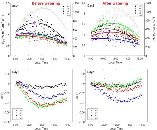
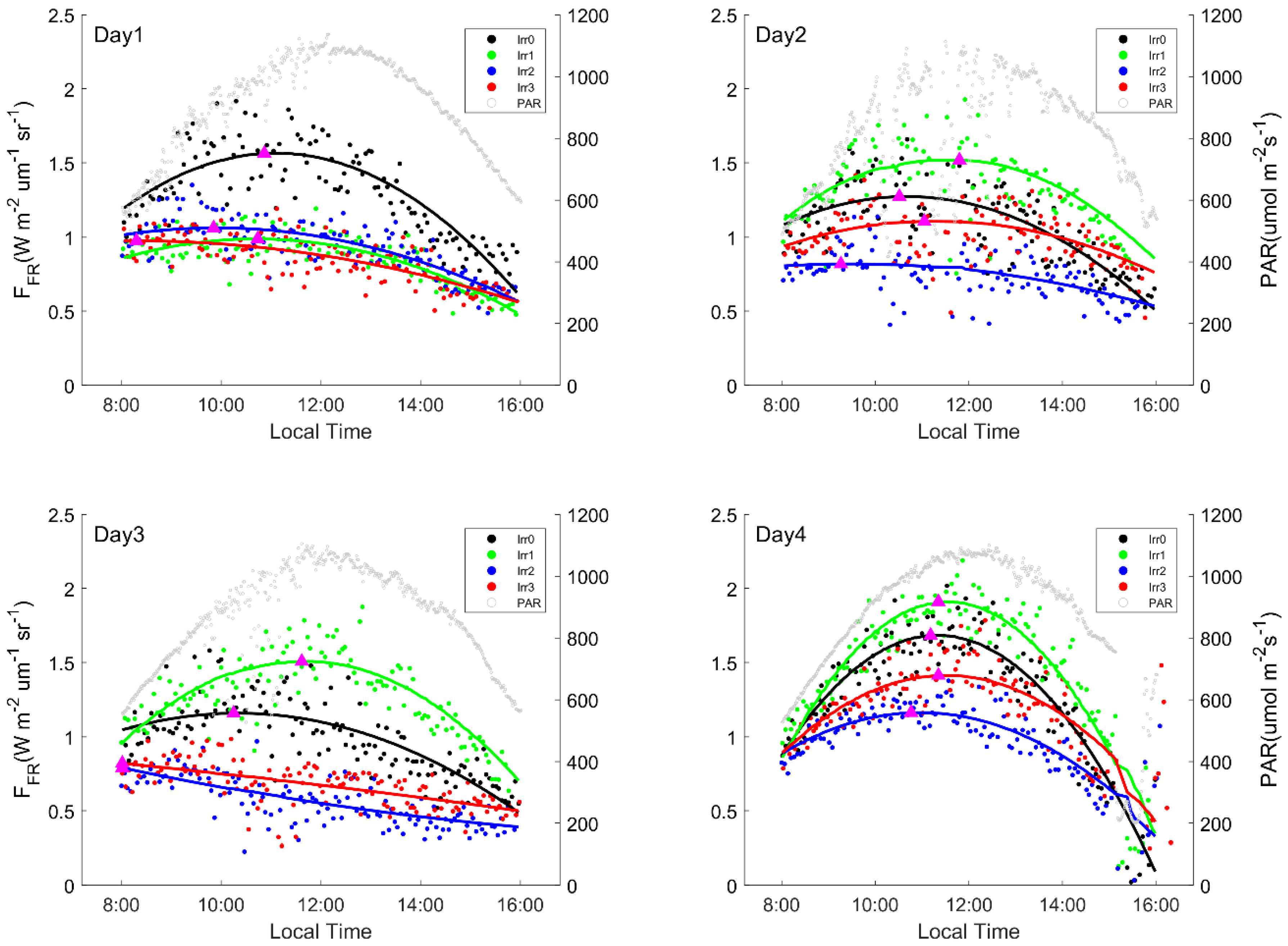
In Figure 2, the measured diurnal FFR, PAR and fitted FFR data are shown. According to the diurnal PAR of the four days, it is clear that the weather was sunny and steady for most of the observation period. When the incoming light was unstable, both FR and FFR varied with the PAR (Figure 2 and Figure 3). The FFR values are consistent with the prior irrigation amount (Irr0 > Irr2 > Irr1 = Irr3) in Figure 1 on Day1. In Figure 2 and Figure 3, quadratic polynomial was used to fit measured data and the R2 of the fittings for Figure 2 and Figure 3 were shown in Tables S1 and S2. From the fitted data, it is clear that under drought conditions, FFR decreased, and the peak times advanced. The magnitude of the advance increased with the severity of the drought. The peaks appeared as early as 8 o’clock to 9 o’clock (Figure 2 Day1). After re-watering on the evenings of 30 July and 3 August, the FFR values of those that were watered exhibited an obvious increase. When the drought eased, the size of FFR changed synchronously with PAR and reached its maximum at noon, as shown in Figure 2 Day4.
Due to the weak canopy fluorescence and narrow absorption band at the O-B band, the estimated FR data are noisier than the FFR data. Therefore, these data were smoothed using the nearest three values, and the results are shown in Figure 3. The values of FR were smaller than those of FFR. During drought, FR also decreased. However, unlike FFR, the peak of FR did not advance and still occurred at noon.
PRI can also characterize water stress, as shown in Figure S1. It is clear that PRI increased after watering. Compared with (Figure 4), there were some differences in the order of the values. For example, the PRI value of Irr1 was larger than that of Irr3 on the Day1, but they had the same irrigation amount. The main reason for this was that LAI had a non-negligible effect on the canopy PRI. To eliminate this effect, the relative change in PRI, that is, , was better for comparing the changes in PRI with different LAI values.
On a given day, started to decrease from 8:00 until approximately 13:00 and then increased at different magnitudes for different water conditions (Figure 4). For Irr0, which had a higher soil water content and LAI value, its exhibited only a slight decrease near midday, and its PRI maintained a range from approximately 0 to −0.01 all day long. For the water-stressed plots, declined steeply in the morning and started to increase gradually after 13:00, but it could not recover to its original value in the morning. By noon, the difference between the dry and non-dry values was greatest and lasted until 16:00. After watering, had a remarkable response and showed similar patterns as Irr0, as shown in Figure 4 Day2. The time when reached its minimum during a day did not change significantly with different water stress conditions.
During the experiment, the air temperature generally increased from 8:00 to 16:00. Most of the time, rose and then fell during a day, reaching a maximum at approximately 13:00. In the absence of drought stress, the change range of in a day is small, and the maximum value is no more than 3 °C (e.g., the diurnal of plot Irr0 in Figure 5 Day1). Under drought stress, increased significantly from 8:00 to 13:00. The more severe the stress was, the faster rose. The maximum value of could reach 10 °C (Figure 5). By noon, the difference between dry and non-dry was greatest and lasted until 16:00. After watering, obviously decreased, as shown in Figure 5 (Day2, Day4). can be a efffective indicator of stomatal cluosure. So there were differences between morning and after noon in stomatal closure for those plots.
3.2. Diurnal SIF/PAR and SIF Yield
As shown in Figure 2 and Figure 3, the SIF values were dominated by irradiance. By normalizing the SIF data using PAR, the effects of factors other than irradiance can be shown [26]. Under no water stress, the normalized far red SIF (FFR/PAR) values gradually decreased from 8:00 to 15:00 and then increased (Figure 6). On the afternoon of Day4, the recovery of FFR/PAR was disturbed by cloudy weather. Under drought stress, FFR/PAR decreased more rapidly before 12:00 and then remained stable until it started to recover after 15:00. Unlike FFR/PAR, the daily change trends of FR/PAR (not shown) were not obvious, which may be due to the effects of data noise or FR intrinsic characteristic.
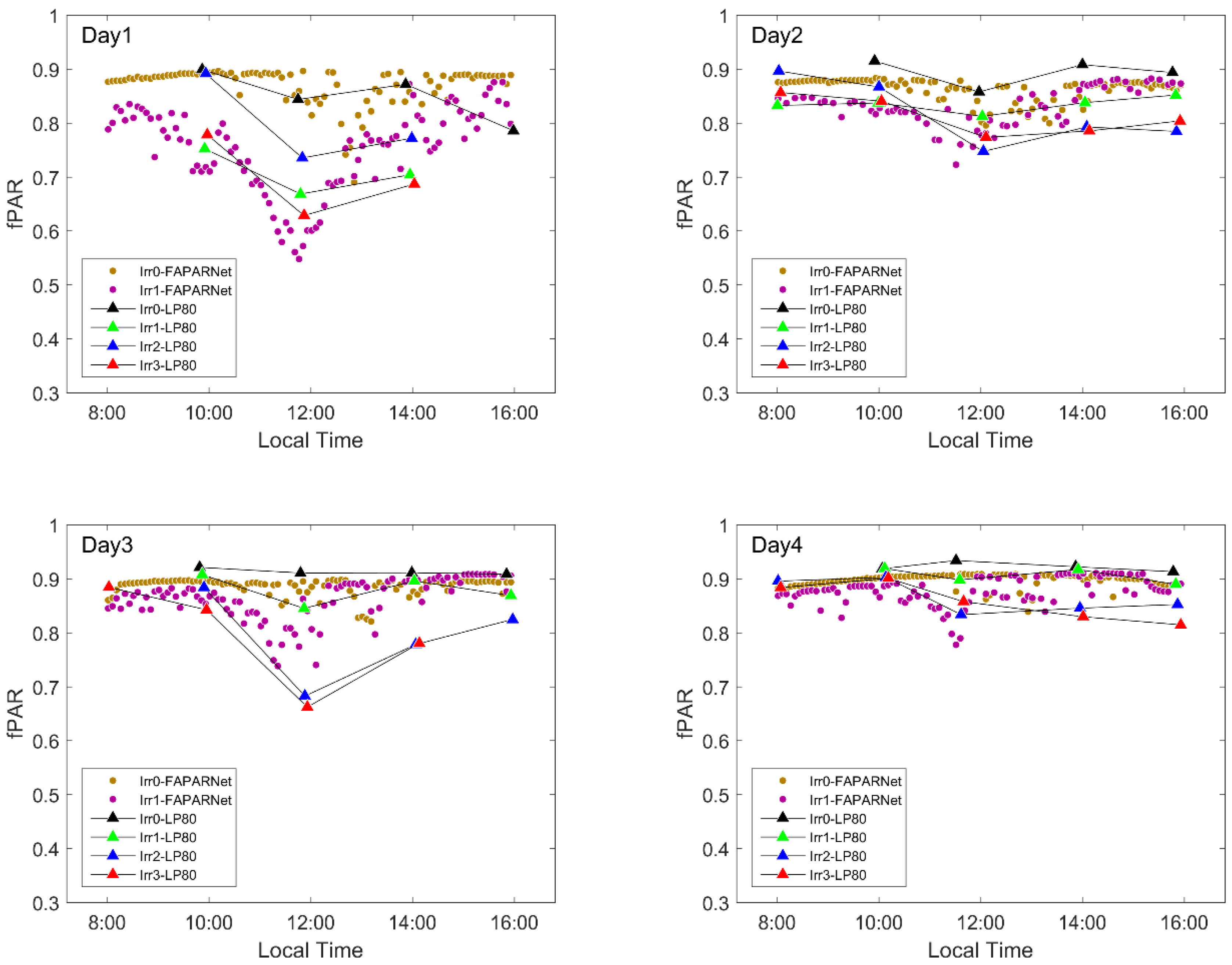
Normalized SIF can be considered to reflect the apparent fluorescence emission efficiency, which is the combination of the ability of the canopy to absorb PAR and the ability to convert the absorbed PAR into fluorescence. To distinguish the effects of these two abilities, fPAR data were measured in two ways in this study. An AccuPAR LP-80 was used to measure fPAR for all plots five times a day. A FAPARNet was used to continuously measure fPAR for plot Irr0 and Irr1 at high frequency. Although the sampling frequencies were different, the daily variation trends of the results of these two methods were consistent (Figure 7). These results show that fPAR declined at noon, when more sunlight reached the ground at noon and was absorbed and reflected by soil. These observed decreases increased under drought. During drought, the maize leaves gradually wilted in the morning as the light increased. As the leaves wilted, the effective leaf area gradually decreased. This resulted in more direct sunlight reaching the ground.
To analyze the change in the ability to convert the absorbed PAR into fluorescence, the SIF yields of plots Irr0 and Irr1 were calculated by normalizing the SIF data using APAR data, which were estimated by the high-frequency fPAR collected by the FAPARNet (Figure 8). The FFR yield and FR yield both decreased from morning until approximately 15:00, but the slopes of these decreases in yield were different. The FFR yield decreased faster than the FR yield. In Figure 8 Day1 for Irr1, obvious ‘bulges’ occur at midday. There may be two reasons why the SIF yield increased significantly at noon. The first is physiological changes. The second one is that the fPAR data measured at noon cannot reflect the true absorption of chlorophyll [27]. Further research is needed to determine the real reason.
3.3. Leaf
YII indicates the quantum yield of linear electron flux (LEF) through the PSII reaction centers, which can be used to represent the PSII operating efficiency under different environmental conditions [28]. The values of YII measured in leaves by PAM2500 are shown in Figure 9. The diurnal YII values of the Irr0 plot, which has no drought stress, decreased slightly from 8:00 to midday and then increased. Under drought stress, the YII values are smaller and decreased faster than those of the plots without stress. YII significantly increased after irrigation. It isn’t clear that the change pattern of Day3 was different other days. There are some abnormal data, which resulted from cloudy sky conditions, such as those observed at 10:00 in Figure 9 Day2 and 16:00 in Figure 9 Day4. Because the photochemical yield will increase under low-light conditions [29], YII showed a steep increase when it was cloudy.
Figure 10 shows the relationship between the leaf YII and the canopy or FFR yield at different times for four days. Due to the same diurnal trend of and PRI, was chosen to study the relationship. The two scatter plots have a good linear relationship after 8:00. In the afternoon, there were higher values of , which means that PRI can better respond to the PSII operating efficiency during this time. The relationship between YII and the FFR yield was significant but weaker () than that of PRI. Consistent with PRI, the FFR yield also had higher values from 10:00 to 14:00.
4. Discussion
Plants have a range of response mechanisms that they use to cope with the stress imposed by a water deficit. Changes in the canopy structure and physiology are the main mechanisms in this coping process; this framework is shown in Figure 11. In this study, water stress was imposed on maize, which then recovered, and both physiology and structure information were measured to determine how they changed.
On the one hand, leaf folding occurs to reduce water evapotranspiration under water stress. Leaf folding directly leads to a decrease in LAI. In this research, for instance, the LAI of Irr1 significantly increased from 2.18 to 3.13 after watering on the evening of Day1. If we assume that true LAI values do not change overnight, then it can be inferred that the LAI difference of Irr1 was caused by leaf folding. In addition, leaf folding can also cause a decrease in fPAR. From Figure 7, it is clear that fPAR underwent an obvious increase after watering on Day1 and Day3. Furthermore, changes in LAI and fPAR will have effects on the measurements reflecting physiological information, including PRI and SIF.
On the other hand, changes in inner physiology occur to ease the influence of water deficit. Blade stomata closure and Non-photochemical Quenching (NPQ) can be used as two effective methods from a physiological perspective. Moreover, changes in stomatal conductance as a result of stomatal closure will influence NPQ.
First, stomata closure occurs to prevent water vapor loss. As the main channel for the exchange of water and carbon dioxide, stomata closure will cause the leaf temperature to increase and the leaf intercellular carbon dioxide concentration to decrease. Thus, leaf or canopy temperature can be used as an alternative to stomatal conductance [30]. The values of (canopy temperature) were higher under stress than they were under stress easing during this experiment. The results indicated canopy temperature did a great job detecting the water stress and identifying the different water regimes. However, water stress does not only affect stomatal closure, but also light absorption and light energy distribution to prevent the formation of reactive oxygen species (ROS) which can damage plants [30]. And SIF or PRI is efficient in monitoring light energy distribution process, for example NPQ and PQ.
Second, Non-photochemical Quenching (NPQ) will increase to cope with stress. Since heat dissipation (NPQ), chlorophyll fluorescence and photosynthesis (or Photochemical Quenching, PQ) compete with each other for the use of absorbed light, plants can actively adjust their energy distribution to adapt to the environment [18,23,26]. NPQ is used by plants as a process to protect against excess energy. Once activated, NPQ will become the primary mechanism. Because fluorescence and photochemical yields are affected by NPQ, changes in NPQ will lead to changes in these two yields.
In this study, at the leaf scale, we estimated the PSII operating efficiency (YII) to examine photochemical variations. YII first decreases and then increases during a day, and the lowest point occurs at midday. Under water stress, YII exhibited a significant decrease. These two decreases are both affected by the increase in NPQ.
At the canopy scale, SIF and PRI were used to study changes in NPQ. PRI was directly related to the pH-dependent NPQ, which has the highest share of all types of NPQ [19]. However, canopy PRI is sensitive to the canopy structure, such as LAI. From this study, we know that PRI values showed obvious differences under the same irrigation conditions. For example, the Irr1 and Irr3 PRI were different because of their different LAI on Day1. Therefore, we used the relative diurnal PRI change to eliminate the effects of canopy structure. reflects changes in NPQ well. Under water stress, this value decreased compared to that obtained after re-watering. During a day, it first decreases at noon and then increases in the afternoon. However, it did not return to its value in the early morning, as PAR decreased under stress. The main reason for this pattern is the reduced photosynthetic capacity under water stress. As Figure 9 shows, for stressed plots, YII continued to decrease from morning to noon, and then a partial recovery in the afternoon except for Day3.
In addition, the SIF, normalized SIF by PAR and SIF yield also exhibited special diurnal variations at the -A and -B bands for different water stress conditions because of the NPQ. In the -A band, for stressed plots FFR achieved a maximum at low PAR, which is consistent with that observed in previous work [31], but FR increased with PAR until noon. At the canopy scale, the SIF intensity can be affected by both the canopy structure and NPQ. The parameters of canopy structure, including LAI and the leaf angle inclination distribution, are very important for SIF emission and transfer. First, absorbed photosynthetically active radiation plays a decisive role that is dominated by LAI and leaf angle inclination distribution. In addition, the plant effective LAI and leaf angle inclination will change under drought. Thus, the canopy SIF will change with changes in the canopy structure. In this study, FFR sharply decreased compared to that observed with no water stress as a result of LAI and leaf inclination changes. During a day, the degree of leaf folding gradually increases from morning to midday, which will lead to effective LAI gradually decrease. So the decrease of LAI can lead to reach the peak at earlier hours in water stressed plants. For FR, fluorescence can be reabsorbed within leaves and the canopy [10], which means that the greater the LAI is, the stronger the reabsorption is. Therefore, when the effective LAI decreases, the effect of reabsorption becomes weak. Canopy structure may be the main reason for the different change patterns between FFR and FR. What more, FR is only emitted from the PSII while FFR is emitted by both photosystems. This difference can also have important physiological implications which may lead to their different change patterns. At diurnal scale, Agati indicated that the ratio between FR and FFR varies in response to the action of NPQ [32]. In this study, the ratio has a special diurnal pattern, but there is no difference between different water stresses. It had an increase from morning to midday and then had a slightly decrease as shown in Figure S2. Thus, the ratio is insensitive in response to water stress at canopy scale. Second, SIF yield can be an indicator of physiological status. The FFR yield and FR yield both decrease from morning to approximately 15:30 in the afternoon, but the slope and magnitude of the decrease in yield are different for the FR yield and FFR yield. As the model results obtained by C. van der Tol demonstrated [29], the steady state yield decreases with increasing irradiance under higher light and drought conditions. In addition, drought will decrease the carboxylation ability of the plant, which can be represented by the maximum carboxylation capacity (Vcmo) in the model. In this study, the SIF yield is consistent with the simulation results obtained using different Vcmo values modeled by C. van der Tol [29]. This is one reason why FFR reaches a maximum at lower PAR for drought plots. For the different change pattern of FFR and FR, further research is needed to study the effect of canopy structure and NPQ on them.
However, the relationship between FFR yield and leaf YII or photosynthetic efficiency is complex and is not a simple linear relationship at different times, as shown in Figure 10. The diurnal FFR yield at the canopy is complicated by the mixed effect of the canopy structure and changes in the solar zenith angle. This mixed effect can have a non-negligible effect on APAR or fPAR. Therefore, in this study, SIF yielded an apparent fluorescence parameter with both physiological and canopy structure information. To eliminate the canopy structure effect, using a canopy radiation transfer model to estimate true APAR is necessary and effective.
In monitoring water stress, it is easy to distinguish whether maize suffer from water stress from SIF and PRI. However, the above results show that PRI, SIF, and SIF yield exhibit dynamic responses to environment conditions. In addition, a series of changes occur at different stages for plants, such as the canopy structure and concentrations of photosynthetic pigments, which play important roles in determining the magnitudes of SIF and PRI [12,33]. Therefore, it is difficult to predict whether plants will suffer from drought using only one or several measurements of PRI and SIF during a day if we do not have control treatment plots. A viable approach to detecting drought is using time series measurements, which can be high-frequency time series measurements during a day or multi-day time series measurements. Using high-frequency time series measurements, we can use different indicators to monitor water stress at different times, as shown in Figure 10.
5. Conclusions
The work presented in this manuscript examined the diurnal responses of SIF and PRI to different water stress conditions. Using the Automatic Observation System, the continuous diurnal dynamics of SIF and PRI were captured at the canopy level. The diurnal dynamics of these parameters before and after watering at the jointing stage were compared.
Our results demonstrate that both the canopy SIF and PRI can dynamically reflect physiological status information under changing environmental conditions on the diurnal scale. First, the diurnal variations in FR and FFR at the canopy scale have different change patterns. Although both FR and FFR decrease under a water deficit, FR always peaked at midday, and the peak of FFR arrived earlier with the increase in water stress. The leaf YII values under drought conditions were also smaller than those of the controlled plots, and all plots of diurnal leaf YII gradually decreased from 8:00 to 14:00 and then recovered. In addition, the canopy structure changes because leaf folding affects APAR and SIF emissions. Thus, the canopy SIF and SIF yield were affected by changes in the NPQ and canopy structure. Second, the water-stressed and controlled plots had different diurnal PRI variation patterns. The diurnal curves of from 8:00 to 16:00 were symmetric concave curves and showed minor changes compared to the controlled plots. Under water stress, decreased rapidly from 8:00 to 13:00, and the maximum range of this decrease was approximately 0.05. Although the values gradually increased after 13:00, their values at 16:00 were still significantly lower than those at 8:00. The decreased SIF yields, YII, PRI and higher temperature indicate that a higher NPQ occurred after noon. To eliminate the effects of canopy structure on PRI and SIF, the next step will be to quantitatively estimate dynamic variations by combining canopy radiation transfer models and physiological models.
To determine the optimal water stress detection time, it is necessary to find the most obvious responses of SIF and PRI to stress using time series measurements. The presented datasets indicate that SIF performed best in the morning from 10:00 to 14:00, and PRI exhibited a remarkable distinction after midday, as shown in Figure 10. The difference between air temperature and canopy temperature had a good performance in detecting water stress in the afternoon.
Supplementary Materials
The following are available online at https://www.mdpi.com/2072-4292/10/10/1510/s1, Figure S1: during experiment, with Day1 to Day4 representing the 4 observation dates (30 July, 31 July, 3 August, 4 August). On the evening of Day1, Irr1 and Irr3 were watered 0.3 m3 and 0.16 m3, respectively. On the evening of Day3, Irr0, Irr1, Irr2 and Irr3 were watered 0.4 m3, 0.2 m3, 0.3 m3 and 0.16 m3, respectively, Figure S2: The ratio between FR and FFR of Irr0 and Irr1 in Day1, Table S1: The R2 of fitted data about diurnal FFR in Figure 2, Table S2: The R2 of fitted data about diurnal FR in Figure 3.
Author Contributions
Z.L., S.X., L.Z., S.R. and H.Z. performed the experiments; S.X. and Z.L. analyzed the data and wrote the paper.
Funding
This research was funded by the Natural Science Foundation of China (41571409, 41541043) and Jiangxi Provincial Key Laboratory of Soil Erosion and Prevention in China (JXSB201501).
Acknowledgments
We thank Albert Porcar-Castell for comments and suggestions on this manuscript.
Conflicts of Interest
The authors declare no conflict of interest.
References
- Mohammed, G.H.; Goulas, Y.; Magnani, F.; Moreno, J.; Olejníčková, J.; Rascher, U.; Van der Tol, C.; Verhoef, W.; Ač, A.; Daumard, F.; et al. 2012 FLEX/Sentinel-3 tandem mission photosynthesis study. In Final Report. ESTEC Contract No. 4000106396/12/NL/AF; P&M Technologies: Sault Ste. Marie, ON, Canada, 2014. [Google Scholar]
- Lambers, H.; Chapin, F.S.; Pons, T.L. Photosynthesis. In Plant Physiological Ecology; Springer: New York, NY, USA, 2008; pp. 11–99. [Google Scholar]
- Chaves, M.M. Effects of water deficits on carbon assimilation. J. Exp. Bot. 1991, 42, 1–16. [Google Scholar] [CrossRef]
- Zarco-Tejada, P.J.; González-Dugo, V.; Berni, J.A.J. Fluorescence, temperature and narrow-band indices acquired from a UAV platform for water stress detection using a micro-hyperspectral imager and a thermal camera. Remote Sens. Environ. 2012, 117, 322–337. [Google Scholar] [CrossRef] [Green Version]
- Flexas, J.; Bota, J.; Cifre, J.; Escalona, J.M.; Galmés, J.; Gulías, J.; Lefi, E.K.; Martínez-Cañellas, S.F.; Moreno, M.T.; Ribas-Carbó, M.; et al. Understanding down-regulation of photosynthesis under water stress: Future prospects and searching for physiological tools for irrigation management. Ann. Appl. Biol. 2015, 144, 273–283. [Google Scholar] [CrossRef]
- Meroni, M.; Rossini, M.; Guanter, L.; Alonso, L.; Rascher, U.; Colombo, R.; Moreno, J. Remote sensing of solar-induced chlorophyll fluorescence: Review of methods and applications. Remote Sens. Environ. 2009, 113, 2037–2051. [Google Scholar] [CrossRef]
- Wieneke, S.; Ahrends, H.; Damm, A.; Pinto, F.; Stadler, A.; Rossini, M.; Rascher, U. Airborne based spectroscopy of red and far-red sun-induced chlorophyll fluorescence: Implications for improved estimates of gross primary productivity. Remote Sens. Environ. 2016, 184, 654–667. [Google Scholar] [CrossRef]
- Damm, A.; Guanter, L.; Paul-Limoges, E.; Van der Tol, C.; Hueni, A.; Buchmann, N.; Eugster, W.; Ammann, C.; Schaepman, M.E. Far-red sun-induced chlorophyll fluorescence shows ecosystem-specific relationships to gross primary production: An assessment based on observational and modeling approaches. Remote Sens. Environ. 2015, 166, 91–105. [Google Scholar] [CrossRef]
- Yu, T.; Sun, R.; Xiao, Z.; Zhang, Q.; Liu, G.; Cui, T.; Wang, J. Estimation of global vegetation productivity from global land surface satellite data. Remote Sens. 2018, 10, 327. [Google Scholar] [CrossRef]
- Porcar-Castell, A.; Tyystjärvi, E.; Atherton, J.; Van der Tol, C.; Flexas, J.; Pfündel, E.E.; Moreno, J.; Frankenberg, C.; Berry, J.A. Linking chlorophyll a fluorescence to photosynthesis for remote sensing applications: Mechanisms and challenges. J. Exp. Bot. 2014, 65, 4065–4095. [Google Scholar] [CrossRef] [PubMed]
- Gamon, J.A.; Penuelas, J.; Field, C.B. A narrow-waveband spectral index that tracks diurnal changes in photosynthetic efficiency. Remote Sens. Environ. 1992, 41, 35–44. [Google Scholar] [CrossRef]
- Magney, T.S.; Vierling, L.A.; Eitel, J.U.H.; Huggins, D.R.; Garrity, S.R. Response of high frequency photochemical reflectance index (PRI) measurements to environmental conditions in wheat. Remote Sens. Environ. 2016, 173, 84–97. [Google Scholar] [CrossRef]
- Ač, A.; Malenovsky, Z.; Olejníčková, J.; Gallé, A.; Rascher, U.; Mohammed, G. Meta-analysis assessing potential of steady-state chlorophyll fluorescence for remote sensing detection of plant water, temperature and nitrogen stress. Remote Sens. Environ. 2015, 168, 420–436. [Google Scholar] [CrossRef] [Green Version]
- Ni, Z.; Liu, Z.; Huo, H.; Li, Z.L.; Nerry, F.; Wang, Q.; Li, X. Early water stress detection using leaf-level measurements of chlorophyll fluorescence and temperature data. Remote Sens. 2015, 7, 3232–3249. [Google Scholar] [CrossRef]
- Sun, Y.; Fu, R.; Dickinson, R.; Joiner, J.; Frankenberg, C.; Gu, L.; Xia, Y.; Fernando, N. Drought onset mechanisms revealed by satellite solar-induced chlorophyll fluorescence: Insights from two contrasting extreme events. J. Geophys. Res. Biogeosci. 2015, 120, 2427–2440. [Google Scholar] [CrossRef] [Green Version]
- Rossini, M.; Panigada, C.; Cilia, C.; Meroni, M.; Busetto, L.; Cogliati, S.; Amadussi, S.; Colombo, R. Discriminating Irrigated and Rainfed Maize with Diurnal Fluorescence and Canopy Temperature Airborne Maps. ISPRS Int. J. Geo-Inf. 2015, 4, 626–646. [Google Scholar] [CrossRef] [Green Version]
- Yoshida, Y.; Joiner, J.; Tucker, C.; Berry, J.; Lee, J.-E.; Walker, G.; Reichle, R.; Koster, R.; Lyapustin, A.; Wang, Y. The 2010 Russian drought impact on satellite measurements of solar-induced chlorophyll fluorescence: Insights from modeling and comparisons with parameters derived from satellite reflectances. Remote Sens. Environ. 2015, 166, 163–177. [Google Scholar] [CrossRef]
- Lee, J.; Berry, J.A.; Van der Tol, C.; Guanter, L.; Damm, A.; Baker, I.T.; Frankenberg, C. Calculations for chlorophyll fluorescence incorporated into the community land model. In Proceedings of the 2014 AGU Fall Meeting, San Francisco, CA, USA, 15–19 December 2014. [Google Scholar]
- Porcarcastell, A.; Bäck, J.; Juurola, E.; Hari, P. Dynamics of the energy flow through photosystem II under changing light conditions: A model approach. Funct. Plant Biol. 2006, 33, 229–239. [Google Scholar] [CrossRef]
- Süß, A.; Hank, T.; Mauser, W. Deriving diurnal variations in sun-induced chlorophyll-a fluorescence in winter wheat canopies and maize leaves from ground-based hyperspectral measurements. Int. J. Remote Sens. 2016, 37, 60–77. [Google Scholar] [CrossRef]
- Zhou, X.; Liu, Z.; Xu, S.; Zhang, W.; Wu, J. An automated comparative observation system for sun-induced chlorophyll fluorescence of vegetation canopies. Sensors 2016, 16, 775. [Google Scholar] [CrossRef] [PubMed]
- Meroni, M.; Busetto, L.; Colombo, R.; Guanter, L.; Moreno, J.; Verhoef, W. Performance of spectral fitting methods for vegetation fluorescence quantification. Remote Sens. Environ. 2010, 114, 363–374. [Google Scholar] [CrossRef]
- Sabater, N.; Middleton, E.M.; Malenovsky, Z.; Alonso, L.; Verrelst, J.; Huemmrich, K.F.; Campbell, P.K.E.; Kustas, W.P.; Vicent, J.; Van Wittenberghe, S.; et al. Oxygen transmittance correction for solar-induced chlorophyll fluorescence measured on proximal sensing: Application to the NASA-GSFC fusion tower. In Proceedings of the 2017 IEEE Geoscience and Remote Sensing Symposium (IGARSS), Fort Worth, TX, USA, 23–28 July 2017; IEEE: Piscataway, NJ, USA, 2017. [Google Scholar]
- Gamon, J.A.; Berry, J.A. Facultative and constitutive pigment effects on the Photochemical Reflectance Index (PRI) in sun and shade conifer needles. Isr. J. Plant Sci. 2012, 60, 85–95. [Google Scholar] [CrossRef]
- Alonso, L.; Van Wittenberghe, S.; Amorós-López, J.; Vila-Francés, J.; Gómez-Chova, L.; Moreno, J. Diurnal cycle relationships between passive fluorescence, PRI and NPQ of vegetation in a controlled stress experiment. Remote Sens. 2017, 9, 770. [Google Scholar] [CrossRef]
- Van der Tol, C.; Rossini, M.; Cogliati, S.; Verhoef, W.; Colombo, R.; Rascher, U.; Mohammed, G. A model and measurement comparison of diurnal cycles of sun-induced chlorophyll fluorescence of crops. Remote Sens. Environ. 2016, 186, 663–677. [Google Scholar] [CrossRef]
- Du, S.; Liu, L.; Liu, X.; Hu, J. Response of canopy solar-induced chlorophyll fluorescence to the absorbed photosynthetically active radiation absorbed by chlorophyll. Remote Sens. 2017, 9, 911. [Google Scholar] [CrossRef]
- Baker, N.R. Chlorophyll fluorescence: A probe of photosynthesis in vivo. Ann. Rev. Plant Biol. 2007, 59, 89–113. [Google Scholar] [CrossRef] [PubMed]
- Van der Tol, C.; Berry, J.A.; Campbell, P.K.E.; Rascher, U. Models of fluorescence and photosynthesis for interpreting measurements of solar induced chlorophyll fluorescence. J. Geophys. Res. Biogeosci. 2014, 119, 2312–2327. [Google Scholar] [CrossRef] [PubMed]
- Urban, L.; Aarrouf, J.; Bidel, L.P. Assessing the effects of water deficit on photosynthesis using parameters derived from measurements of leaf gas exchange and of chlorophyll a fluorescence. Front. Plant Sci. 2017, 8, 2068. [Google Scholar] [CrossRef] [PubMed]
- Daumard, F.; Champagne, S.; Fournier, A.; Goulas, Y.; Ounis, A.; Hanocq, J.-F.; Moya, I. A field platform for continuous measurement of canopy fluorescence. IEEE Trans. Geosci. Remote Sens. 2010, 48, 3358–3368. [Google Scholar] [CrossRef]
- Agati, G.; Mazzinghi, P.; Fusi, F.; Ambrosini, I. The F685/F730 chlorophyll fluorescence ratio as a tool in plant physiology: Response to physiological and environmental factors. J. Plant Physiol. 1995, 145, 228–238. [Google Scholar] [CrossRef]
- Cogliati, S.; Rossini, M.; Julitta, T.; Meroni, M.; Schickling, A.; Burkat, A.; Pinto, F.; Racher, U.; Colombo, R. Continuous and long-term measurements of reflectance and sun-induced chlorophyll fluorescence by using novel automated field spectroscopy systems. Remote Sens. Environ. 2015, 164, 270–281. [Google Scholar] [CrossRef]
Figure 1.
Experimental field area and automatic observation system.

Figure 2.
Diurnal far red fluorescence (FFR) data, with Day1 to Day4 representing the 4 observation dates (30 July, 31 July, 3 August, 4 August). Scatter points represent measured data, and the solid line represents fitted data of Sun-induced Fluorescence (SIF). Magenta triangles represents peak value of fitted data. On the evening of Day1, Irr1 and Irr3 were watered 0.3 m3 and 0.16 m3, respectively. On the evening of Day3, Irr0, Irr1, Irr2, and Irr3 were watered 0.4 m3, 0.2 m3, 0.3 m3, and 0.16 m3, respectively.

Figure 3.
Diurnal red fluorescence (FR) data, with Day1 to Day4 representing 4 observation dates (30 July, 31 July, 3 August, 4 August). Scatter points represent measured data, and solid line represents fitted data of SIF. Magenta triangles represents peak value of fitted data. On the evening of Day1, Irr1 and Irr3 were watered 0.3 m3 and 0.16 m3, respectively. On the evening of Day3, Irr0, Irr1, Irr2, and Irr3 were watered 0.4 m3, 0.2 m3, 0.3 m3, and 0.16 m3, respectively.

Figure 4.
during experiment, with Day1 to Day4 representing the 4 observation dates (30 July, 31 July, 3 August, 4 August). On the evening of Day1, Irr1 and Irr3 were watered 0.3 m3 and 0.16 m3, respectively. On the evening of Day3, Irr0, Irr1, Irr2 and Irr3 were watered 0.4 m3, 0.2 m3, 0.3 m3 and 0.16 m3, respectively.

Figure 5.
Differences between diurnal variations in canopy temperature and air temperature () during the experiment, with Day1 to Day4 representing the four observation dates (30 July, 31 July, 3 August, 4 August). On the evening of Day1, Irr1 and Irr3 were watered 0.3 m3 and 0.16 m3, respectively. On the evening of Day3, Irr0, Irr1, Irr2, and Irr3 were watered 0.4 m3, 0.2 m3, 0.3 m3, and 0.16 m3, respectively.


Figure 6.
Diurnal variations in far red SIF (FFR) normalized by photosynthetic active radiation (PAR) during the experiment, with Day1 to Day4 representing the four observation dates (30 July, 31 July, 3 August, 4 August). On the evening of Day1, Irr1 and Irr3 were watered 0.3 m3 and 0.16 m3, respectively. On the evening of Day3, Irr0, Irr1, Irr2, and Irr3 were watered 0.4 m3, 0.2 m3, 0.3 m3, and 0.16 m3, respectively.

Figure 7.
Diurnal variations in absorbed PAR (fPAR) during the experiment, with Day1 to Day4 representing four observation dates (30 July, 31 July, 3 August, 4 August). The fPAR data measured by AccuPAR LP-80 are symbolized using LP80. The postfix FAPARNet represents the high-temporal-frequency fPAR data in plots Irr0 and Irr1.

Figure 8.
Diurnal variations in SIF yield (760 nm, 687 nm) for Irr0 and Irr1 plot in 30 July and 31 July. The two pictures above represent the plot Irr0. The two pictures below represent the plot Irr1. For these two plots, we use a continuous measurement device to obtain high-frequency fPAR data.
Figure 8.
Diurnal variations in SIF yield (760 nm, 687 nm) for Irr0 and Irr1 plot in 30 July and 31 July. The two pictures above represent the plot Irr0. The two pictures below represent the plot Irr1. For these two plots, we use a continuous measurement device to obtain high-frequency fPAR data.

Figure 9.
Diurnal variations in photosystem II operating efficiency (YII) during the experiment, with Day1 to Day4 representing the four observation dates (30 July, 31 July, 3 August, 4 August, respectively).
Figure 9.
Diurnal variations in photosystem II operating efficiency (YII) during the experiment, with Day1 to Day4 representing the four observation dates (30 July, 31 July, 3 August, 4 August, respectively).

Figure 10.
The relationship between FFR yield and YII. To explore the correlation between these data at different times, linear fitting was conducted every two hours.
Figure 10.
The relationship between FFR yield and YII. To explore the correlation between these data at different times, linear fitting was conducted every two hours.

Figure 11.
The framework of how plants cope with water stress. The dotted line indicates an indirect effect. Ellipses indicate measurable data.
Figure 11.
The framework of how plants cope with water stress. The dotted line indicates an indirect effect. Ellipses indicate measurable data.


Table 1.
Water regimes of 4 plots. Irrigation was conducted at night on Day1 (30 July) and Day3 (3 August). The cumulative amount prior to measuring represents the total irrigation amount at different growth stages before the field campaign.
Table 1.
Water regimes of 4 plots. Irrigation was conducted at night on Day1 (30 July) and Day3 (3 August). The cumulative amount prior to measuring represents the total irrigation amount at different growth stages before the field campaign.
| Plots | Cumulative Amount Prior to Measuring | Day1 | Day2 | Day3 | Day4 |
|---|---|---|---|---|---|
| Irr0 (m3) | 0.9 | -- | -- | 0.4 | -- |
| Irr1 (m3) | 0.48 | 0.3 | -- | 0.2 | -- |
| Irr2 (m3) | 0.8 | -- | -- | 0.3 | -- |
| Irr3 (m3) | 0.48 | 0.16 | -- | 0.16 | -- |
Table 2.
Leaf area index (LAI) values and chlorophyll contents of every plot during the experiment. Effective LAI values were estimated using the measurements of AccuPAR LP-80 at 10 a.m.
Table 2.
Leaf area index (LAI) values and chlorophyll contents of every plot during the experiment. Effective LAI values were estimated using the measurements of AccuPAR LP-80 at 10 a.m.
| Date | Day1 | Day2 | Day3 | Day4 | |
|---|---|---|---|---|---|
| Effective LAI | Irr0 | 5.74 | 5.48 | 5.94 | 5.79 |
| Irr1 | 2.18 | 3.13 | 3.39 | 3.49 | |
| Irr2 | 4.14 | 3.56 | 3.84 | 4.53 | |
| Irr3 | 2.5 | 2.9 | 3.11 | 3.3 | |
| Relative Chlorophyll content (no unit) | Irr0 | 36.18 | -- | 34.51 | -- |
| Irr1 | 38.05 | -- | 36.84 | -- | |
| Irr2 | 32.32 | -- | 34.14 | -- | |
| Irr3 | 38.79 | -- | 35.04 | -- | |
© 2018 by the authors. Licensee MDPI, Basel, Switzerland. This article is an open access article distributed under the terms and conditions of the Creative Commons Attribution (CC BY) license (http://creativecommons.org/licenses/by/4.0/).
Share and Cite
MDPI and ACS Style
Xu, S.; Liu, Z.; Zhao, L.; Zhao, H.; Ren, S. Diurnal Response of Sun-Induced Fluorescence and PRI to Water Stress in Maize Using a Near-Surface Remote Sensing Platform. Remote Sens. 2018, 10, 1510. https://doi.org/10.3390/rs10101510
AMA Style
Xu S, Liu Z, Zhao L, Zhao H, Ren S. Diurnal Response of Sun-Induced Fluorescence and PRI to Water Stress in Maize Using a Near-Surface Remote Sensing Platform. Remote Sensing. 2018; 10(10):1510. https://doi.org/10.3390/rs10101510
Chicago/Turabian StyleXu, Shan, Zhigang Liu, Liang Zhao, Huarong Zhao, and Sanxue Ren. 2018. "Diurnal Response of Sun-Induced Fluorescence and PRI to Water Stress in Maize Using a Near-Surface Remote Sensing Platform" Remote Sensing 10, no. 10: 1510. https://doi.org/10.3390/rs10101510
Note that from the first issue of 2016, this journal uses article numbers instead of page numbers. See further details here.