Assessment of Multi-Source Evapotranspiration Products over China Using Eddy Covariance Observations

Abstract

As an essential variable in linking water, carbon, and energy cycles, evapotranspiration (ET) is difficult to measure. Remote sensing, reanalysis, and land surface model-based ET products offer comprehensive alternatives at different spatio-temporal intervals, but their performance varies. In this study, we selected four popular ET global products: The Global Land Evaporation Amsterdam Model version 3.0a (GLEAM3.0a), the Modern Era Retrospective-Analysis for Research and Applications-Land (MERRA-Land) project, the Global Land Data Assimilation System version 2.0 with the Noah model (GLDAS2.0-Noah) and the EartH2Observe ensemble (EartH2Observe-En). Then, we comprehensively evaluated the performance of these products over China using a stratification method, six validation criteria, and high-quality eddy covariance (EC) measurements at 12 sites. The aim of this research was to provide important quantitative information to improve and apply the ET models and to inform choices about the appropriate ET product for specific applications. Results showed that, within one stratification, the performance of each ET product based on a certain criterion differed among classifications of this stratification. Furthermore, the optimal ET (OET) among these products was identified by comparing the magnitudes of each criterion. Results suggested that, given a criterion (a stratification classification), the OETs varied among stratification classifications (the selected six criteria). In short, no product consistently performed best, according to the selected validation criterion. Thus, multi-source ET datasets should be employed in future studies to enhance confidence in ET-related conclusions.

1. Introduction

As an essential component of water balance, evapotranspiration (ET) can directly impact both regional and global hydrological processes. Globally, ET has changed over recent decades, owing to climate and vegetation changes, human activities, and other factors [1,2,3]. Additionally, ET plays a crucial role in the land–atmosphere interface, which is closely associated with various climate variables (e.g., humidity, cloud information, temperature, and precipitation) given its link with water, energy, and carbon cycles, thus further influencing the climate system [4,5]. Accurate estimation of ET is crucial to comprehensively understand the changes in regional and global hydrological cycles (including extreme events, such as floods and droughts) and climate, and to reasonably and accurately estimate ecosystem productivity and agricultural irrigation needs [6,7,8,9]. More importantly, this information is of practical significance for food security and sustainable development of the global socio-economy [10,11].

Despite its importance, direct and continuous measurements of ET are challenging [4,12,13]. With the development of theories on boundary layer meteorology and observation technology, short-term ET measurements have become available based on porometry and lysimeters [14], energy balance and micrometeorological techniques, such as the Bowen ratio [15], eddy covariance (EC) techniques [16], and scintillometry [17]. Undoubtedly, these measurements provide necessary materials for investigating ET processes and relevant mechanisms, as well as ET-related issues at specific locations and periods; however, owing to the sparse distribution of the observation sites and the shorter time span, the conclusions based on the limited ET observations may lack universality, especially for long time periods and for a large spatial span [8,18]. To that end, numerous remote sensing [19,20,21,22,23], reanalysis [24,25,26,27], and land surface model (LSM)-based ET products [28,29,30], as well as estimates from empirical up-scaling of in situ observations [31] with different spatio-temporal resolutions and spans have recently been developed. While these datasets provide an opportunity for use in long-term and large spatial ET-related studies, validations and inter-comparisons of the data are necessary. Usually, these ET products have different levels of uncertainties, which are associated with their distinct purposes and applications [5,7,32,33,34]. It is reported that the accuracy of remote sensing-based ET varies over space and time, with uncertainties between 15% and 30% [32,33]. Thus, to reduce the impacts of ET product uncertainties on the degree of confidence for ET-related results (e.g., hydrological cycle, land-atmosphere interaction, agriculture, and ecosystem), we should assess the suitability of the ET products.

Eddy covariance (EC) ET has been used as the typical reference data for validating various ET estimates at the site and pixel level (e.g., for a remote sensing-based product) or at grid (e.g., reanalysis- and LSM-based products) scales [4,35,36]. Yet, EC measurements are commonly flawed, particularly with respect to a lack of energy balance closure at some EC sites, relatively short periods, and sparse spatial coverage [37]. Recently, many studies have quantified the performance of various ET products across the globe [5,8,34,38,39,40,41,42]. For example, Michel et al. [40] used EC ET at 24 towers across the world as benchmark data to assess four remote sensing-based ET products, and stated that all of the products performed better in wet and moderately wet climate regimes than in dry regimes. Majozi et al. [8] evaluated the accuracy and precision of four ET estimates over two eco-regions of South Africa, and indicated that none of the ET products always performed better in the two biomes. Kim et al. [38] found that the Moderate Resolution Imaging Spectroradiometer (MODIS) MOD16 ET for forested land cover of Asia was more accurate than for other biomes. Ershadi et al. [34] concluded that the ET models in Europe and North America performed differently for certain biomes, and models with relatively higher accuracy varied among biomes.

The climate in China has greatly changed in recent decades, with obvious variations in precipitation, temperature, wind speed, sunshine duration or radiation, and humidity [43,44,45,46,47,48,49,50,51]. It is worth quantifying how and by what magnitudes the ET processes responded to the climate change in order to formulate climate change countermeasures (e.g., maintaining ecosystem health, planning agricultural irrigation, and reducing natural disasters to the socio-economy). While a number of ET products provide the necessary tools to examine this issue, the potential risks of inaccurate and even incorrect conclusions are still large, owing to a lack of validations of these products. Recently, some assessments have been conducted for various ET products, as well as the robustness of different ET algorithms across China based on limited EC observations [39,52,53,54,55,56,57]. In the work of Yang et al. [42], the validation results for the GLEAM ET showed that, relative to EC ET at eight sites, this product performed well, particularly for the grassland sites. On the basis of routine measurements at one EC site in a semi-arid environment of north China, Schneider et al. [52] analyzed the capabilities of four ET algorithms in estimating ET and suggested that the Hargreaves and Makkink methods outperformed others. Yang et al. [56] evaluated the performance of three dual-source ET products in the Heihe River Basin in Northwest China, and indicated that the MOD16 and HTEM (hybrid dual-source scheme and trapezoid framework-based ET model) ET performed the worst and best, respectively.

Undoubtedly, ET processes and variations are of theoretical significance in the development of disciplines and inter-disciplines and have practical application value for social sectors, especially for China with exacerbating climate change. Therefore, evaluations of existing and newly released ET products (e.g., the EartH2Observe ensemble) from various perspectives (e.g., performance in various biomes and climate regimes and at various elevation levels) are essential for comprehensively documenting the suitability of these available products and further improving them. Such evaluations will provide more accurate ET estimates for ET-related studies, and thus, enhance the robustness of ET-related results. For this purpose, we collected EC observations from 12 sites in China, which generally cover common biomes, climate regimes and elevation levels, and four popular or new ET global products (one remote sensing-based product, one LSM ensemble, and two reanalyzes-based ET products). A stratification method using the whole of all of the EC sites, biomes, climate regimes, and elevation levels was employed to comprehensively validate these products using EC ET as a benchmark reference. Then, the corresponding optimal ET product (OET) was identified by comparing the magnitude of each validation criterion. We will discuss the potential causes for the performance outcomes, as well as various aspects of the product uncertainties.

2. Data and Methods

2.1. Global Land Evaporation Amsterdam Model ET

A remote sensing-based product, the Global Land Evaporation Amsterdam Model (GLEAM) ET was among the products selected for this study. This model comprises a set of algorithms with inputs of various satellite observations and reanalysis forcings (

Table 1. Overview of ET products, including their PET schemes, along with the number of soil layers, precipitation and radiation datasets and other forcings.

ET Products	PET Schemes	Major Forcing Datasets			References
		Precipitation	Radiation	Others
GLEAM3.0a	Priestley-Taylor	MSWEP	ERA-Interim	ESA GLOBSNOW and NSIDC SWE, CCI-LPRM VOD, CCI SM and LIS/OTD LF	Martens et al. [58]
MERRA-Land	Penman-Monteith	CPC-U	MERRA version 1.0 outputs	T, W, Q and SP	Reichle et al. [60]
GLDAS2.0-Noah	Penman-Monteith	PUMFD	PUMFD	T, W, Q and SP	Rodell et al. [28]
EartH2Observe-En	Variable	WFDEI	WFDEI	T, W, Q and SP	Schellekens et al. [30]

Note: MSWEP: Multi-Source Weighted-Ensemble Precipitation; CPC-U: Climate Prediction Center Unified; ESA: European Space Agency; NSIDC: National Snow and Ice Data Center; CCI-LPRM: Climate Change Initiative-Land Parameter Retrieval Model; LIS/OTD LF: Lightning Imaging Sensor/Optical Transient Detector lighting frequency; W: wind speed; Q: relative or specific humidity; SP: surface pressure. Among the EartH2Oberve models, the PET schemes are different, including Penman-Monteith, Bulk ETP, Hamon (tier 1), modified Penman, Priestley-Taylor and net radiation-based algorithms. A detailed description about these models can be found in Dutra et al. [61] and their respective model papers (Table S1).

), whose rationale is to maximize the recovery of information on ET contained in current satellite observations of climate and environmental elements [58]. It separately estimates three sources of ET (transpiration, soil evaporation, and interception) for bare soil, short vegetation, and vegetation with a tall canopy within each grid cell. First, potential ET (PET) was calculated based on the Priestley-Taylor formula and measurements of surface net radiation and near-surface temperature. For each fraction of bare soil, tall canopy, and short canopy, the estimated PET was then converted into actual ET by applying a multiplicative stress factor, which is a function of microwave vegetation optical depth (VOD; [59]) observations and soil moisture (SM) estimates from a multi-layer running water balance. Specifically, to minimize uncertainties from random forcing, satellite-based SM was assimilated into the soil profile. Regarding interception loss, a Gash analytical model was employed by GLEAM. In contrast, ET for water bodies and regions covered by ice and/or snow was obtained by a variant of the Priestley-Taylor equation. Three new datasets of ET with different forcings and spatio-temporal coverage were produced by GLEAM version 3.0 (v3.0). The GLEAM v3.0a (GLEAM3.0a) ET product was chosen because of the valuable potential of this data in climate change studies, given that the datasets have the longest temporal and the largest spatial spans of 1980–2014. This daily datasets have a spatial resolution of 0.25° × 0.25° and are based on satellite-observed SM, VOD, and snow-water equivalent (SWE), reanalysis air temperature (T) and radiation, and a multi-source precipitation product.

2.2. Modern Era Retrospective-Analysis for Research and Applications-Land ET

The Modern Era Retrospective-Analysis for Research and Applications (MERRA)-Land ET is a reanalysis-based product. MERRA is an addition to the suite of global, long-term reanalysis products generated by the National Aeronautics and Space Administration (NASA) Global Modeling, and Assimilation Office (GMAO) with the Goddard Earth Observing System (GEOS-5; [62]). This system combines the NASA Atmospheric General Circulation Model (AGCM) with a set of state-of-the-art physics packages and the National Centers for Environmental Prediction (NCEP) Gridpoint Statistical Interpolation (GSI) assimilation package, and incorporates information from ground and satellite-based observations of the atmosphere, including many modern satellite derivations (e.g., Atmospheric Infrared Sounder (AIRS) radiances and scatterometer-based wind retrievals). In particular, MERRA focuses on historical analyses of the hydrological cycle on a broad range of weather and climate time scales, and thus introduces the innovative GEOS-5 Catchment LSM [63], which can explicitly address the subgrid-scale SM variability and its impact on runoff and ET. Unlike common LSMs, this model is run at the basic computational unit of the topographically determined hydrological catchment or watershed. For the original MERRA, the precipitation is simulated from the system’s AGCM following the assimilation of the atmospheric observations; however, significant errors exist in the amounts and timing of the model-generated precipitation and negatively influence the land surface hydrological variables [26]. To overcome this issue, offline, land-only reanalysis data (i.e., MERRA-Land) were produced based on merging gauge-based data from the NOAA Climate Prediction Center with MERRA precipitation and revised parameters in the original canopy precipitation interception model. This supplemental land surface data of the original MERRA, as noted by Reichle et al. [60], stated that the capability of MERRA-Land in the land hydrology estimates has been significantly improved. The monthly MERRA-Land ET, with a horizontal grid of 0.67° longitude × 0.5° latitude, is used here and covers the period from 1980–2016.

2.3. Global Land Data Assimilation System ET

The Global Land Data Assimilation System (GLDAS) is based on the North American Land Data Assimilation System (NLDAS), and is a global, high-resolution, offline (uncoupled to the atmosphere) terrestrial modeling system together with data assimilation techniques for producing fields of land surface states and fluxes (e.g., ET, SM, and latent, sensible, and ground heat flux) in near-real time. Importantly, for more optimal land surface products from different LSMs (i.e., Mosaic, Noah, the Community Land Model, and the Variable Infiltration Capacity model), the satellite and ground-based observations are used as constraints in both model forcing (to avoid biases in atmospheric model-based forcing) and parameterization (to curb unrealistic model states; [28]). To date, two versions of the GLDAS product (i.e., GLDAS1.0 and GLDAS2.0) have been released. Recently, increasing evidence has reported that GLDAS1.0 products have serious discontinuity issues owing to their forcing data (e.g., with large precipitation and temperature errors in 1996 and 2000–2005, respectively) [64]. Therefore, we use the monthly ET from the GLDAS2.0 coupled with the Noah LSM (GLDAS2.0-NOAH), which has a spatial resolution of 0.25° × 0.25°. This product is simulated using the Princeton University meteorological forcing dataset (PUMFD), which has been bias corrected via observation-based products for the period 1948–2010 [65].

2.4. EartH2Observe ET

Aiming to develop a global water resources reanalysis for multi-scale water resource assessments and research projects, the EartH2Observe project uses state-of-the-art meteorological reanalysis and five global hydrological models (GHMs), a simple water balance model, and four LSMs with extended hydrological schemes. These models run offline and are driven by the same reanalysis-based forcing (i.e., WATCH (Water and Global Change FP7 project) Forcing Dataset ERA-Interim (WFDEI)) [66]. This dataset is based on the European Centre for Medium-Range Weather Forecasts (ECMWF) ERA-Interim reanalysis and has been adjusted with the Climatic Research Unit (CRU) dataset by a sequential elevation correction of surface meteorological elements plus monthly bias correction from gridded measurements. The simulations were performed from 1979–2012 in a continuous run. It should be noted that because of the different nature of the models, the spin-up procedures differed and were performed respectively to match their requirements and reach the climatic equilibrium states [30]; detailed information about these models can be found in Dutra et al. [61] and in their respective model papers. For an individual model, the daily and monthly simulations of the state of the surface water storage and fluxes are provided at a spatial resolution of 0.5° × 0.5°, as well as the 10-model arithmetic mean (i.e., ensemble). The monthly multi-model ensemble (named EartH2Observe-EN) ET is used in this study, which can mitigate the potential errors and uncertainties from a single model [67].

Notably, in order to make inter-comparison possible, all selected ET products were aggregated to the same spatial resolution (0.25° × 0.25°) with a widely used bilinear interpolation method and temporal (monthly) resolutions. More information about these products is listed in Table 1.

2.5. Eddy Covariance ET

The observed ET (generally reflected by latent heat flux) at 12 EC sites (

Table 2. Overview of EC stations selected to validate ET products.

Full (Abbreviated) Name	Lon (°N)	Lat (°E)	Altitude (m)	Time Span	IGBP Biomes	Precipitation (mm)	PET (mm)	CAI
Changbaishan (Cbs) a	128.10	42.40	738	2003–2005	MF	682.80	667.33	0.99
Qianyanzhou (Qyz) a	115.06	26.74	110.8	2003–2005	ENF	1517.2	995.29	0.65
Dinghushan (Dhs) a	112.54	23.17	300	2003–2005	EBF	1730	1064.2	0.63
Xishuangbanna (Xsbn) b	101.27	21.95	750	2003–2005	EBF	1446.9	1130.1	0.83
Yucheng (Yc) b	116.57	36.83	28	2003–2005	CRO	531.61	822.85	1.49
Haibei Alpine Tibet (Haa) a	101.18	37.37	3250	2002–2004	GRA	428.15	760.93	1.99
Haibei Shrub-land (Has) a	101.33	37.61	3160	2003–2005	WET	433.08	755.62	1.85
Neimenggu (Nmg) b	116.67	44.53	1189	2004–2005	GRA	304.82	703.01	2.39
Dangxiong (Dx) a	91.07	30.50	4333	2004–2005	GRA	405.52	871.01	2.56
Changling (Cl) a	123.51	44.59	171	2007–2010	GRA	404.66	716.59	1.76
Duolun (Dl) a	116.28	42.05	1350	2006–2008	GRA	389.51	730.72	1.91
Shouxian (Sx) c	116.79	32.44	24	2007–2010	CRO	1021.1	918.35	0.92

Note: ^a, ^b and ^c denote that this site is from FLUXNET, ChinaFlux and NCO-CMA, respectively.

and Figure 1), commonly used to monitor CO₂, water vapor, and energy exchanges between the biosphere and atmosphere, were collected to examine the performance of the four ET products. Of these sites, one, eight, and three are from National Climatological Observatory of China Meteorological Administration (NCO-CMA), FLUXNET (http://fluxnet.fluxdata.org/), and ChinaFlux (http://www.chinaflux.org/), respectively. While half-hourly observations were obtained, the time spans of the EC site observations differed, ranging from 2 (24) to 4 years (48 months). Standardized procedures [68] and the gap-filled method [69] were used for quality control of the EC measurements. To obtain consistent temporal resolutions for the four ET products, we also aggregated the EC half-hourly measurements to monthly and annual values at each site for the following analyses. These sites are distributed across different International Geosphere-Biosphere Programme (IGBP)-based biomes (i.e., mixed forest (MF), evergreen needleleaf forest (ENF), evergreen broadleaf forest (EBF), crop-land (CRO), grassland (GRA), and wetland (WET)), climate regimes (arid and wet regions), and elevation levels (>500 m, 500–1500 m, and <1500 m). Notably, the aridity index, which has been widely used to create climate divisions over the globe (e.g., Reference [70]), is employed to define climate regimes here. Arid and wet regions correspond to climatological aridity indices (CAI; climatological value of PET divided by that of precipitation) above and below 1.0, respectively. In this study, CAI is computed based on the gridded monthly PET and observational precipitation with a spatial resolution of 0.25° × 0.25°. PET is calculated from the Food and Agriculture Organization (FAO)-56 Penman-Monteith equation [71] with the gridded monthly meteorological observations (i.e., sunshine duration, wind speed at 2 m height, and maximum and minimum temperatures, and relative humidity). The gridded datasets are produced based on routine meteorological observations at 1211 weather sites of CMA using an inverse distance weighted interpolation method.

To obtain the observed ET (mm/day), the daily EC latent heat flux (LE, W/m²) from the twelve sites can be converted using the following equation [23,71,72]:

$$\mathrm{ET}=\frac{\mathrm{LE}}{\lambda }$$

(1)

where λ is the LE of vaporization with a fixed value of 2.45 MJ/kg. In fact, this parameter changes with temperature [22,73] and potentially influences the accuracy of the estimated EC ET with Equation (1). To measure the impacts of λ, comparisons of the estimated EC ET, with the constant of 2.45 MJ/kg and the variable λ (reflected by a function of temperature [73]), were conducted; detailed information is presented in Table S2. Briefly, the differences between the two estimations for each site were much smaller, implying that the impacts of the λ changes on the estimated EC ET are minimal. Thus, in this study, we do not consider the impacts of the λ changes due to temperature differences among sites. This study focuses on monthly and annual comparisons, and thus the daily EC ET estimates are integrated into monthly and annual values before conducting validations.

2.6. Validation Criteria

Several validation criteria are employed to comprehensively evaluate the performances of the four ET products. Mean Error (ME) provides a way to quantify the biases of the estimates relative to measurements, while Root-Mean-Square-Error (RMSE) can describe the accuracy of estimations. Due to spatio-temporal differences in ET magnitudes, it is difficult to directly compare ET products’ performances among regions and during study periods using ME and RMSE, and therefore their relative values (i.e., RME and RRMSE) are also given. Alongside the criteria above, correlation coefficient (R) and Taylor Score (TS, between 0 and 1.0 [74]) are computed to measure the capability of capturing spatio-temporal ET variability, and the overall performance of each product, respectively. In general, the higher the TS, the better the ET product performs [74]. These validation metrics are expressed as:

$$ME=\frac{1}{n}{{\displaystyle \sum }}_{i=1}^n\left(S_i-O_i\right)$$

(2)

$$RME=\frac{ME}{O}$$

(3)

$$RMSE=\sqrt{\frac{{{\displaystyle \sum }}_{i=1}^n{\left(S_i-O_i\right)}^2}{n}}$$

(4)

$$RRMSE=\frac{RMSE}{O}$$

(5)

$$R=\frac{{{\displaystyle \sum }}_{i=1}^n\left[\left(S_i-S\right)\left(O_i-O\right)\right]}{\sqrt{{{\displaystyle \sum }}_{i=1}^n{(S_i-S)}^2}\sqrt{{{\displaystyle \sum }}_{i=1}^{\mathrm{n}}{(O_i-O)}^2}}$$

(6)

$$TS=\frac{4·\left(1+R\right)}{{\left(\sigma +\frac{1}{\sigma }\right)}^2·\left(1+R_0\right)}$$

(7)

where n represents the sample number; S is the mean of each ET product averaged among n samples, while O is for the observed ET; i denotes the ith sample; R₀ (=1.0 here) is the maximum theoretical R; and σ indicates the standard deviation of a certain ET product normalized by the standard deviation of the observed ET.

Furthermore, the mechanisms of energy and water exchanges between land and atmosphere are complex, and are often accompanied with strong variability in both space and time. Considering the relationships of ET with physical characteristics of land surface [75,76], it is necessary to conduct comprehensive evaluations from various perspectives, e.g., biome, elevation level and climate regime, which will enhance our knowledge on model performances, explaining possible causes and finally improving models. Therefore, we will employ a stratification method using the whole of all of the EC sites, biome, elevation level, and climate regime to conduct analyses of the four ET products in the coming sections. For each stratification, it has different classifications, i.e., 14 (1 for all monthly and annual data, and 12 for monthly data of 12 months) for the whole of all of the EC sites, 6 (MF, ENF, EBF, CRO, GRA, and WET) for biome, 3 (<500 m, 500–1500 m and >1500 m) for elevation level and 2 (wet and dry corresponding to CAI <1.0 and >1.0, respectively) for climate regime. Then, the validation criteria are calculated for each stratification classification.

3. Results

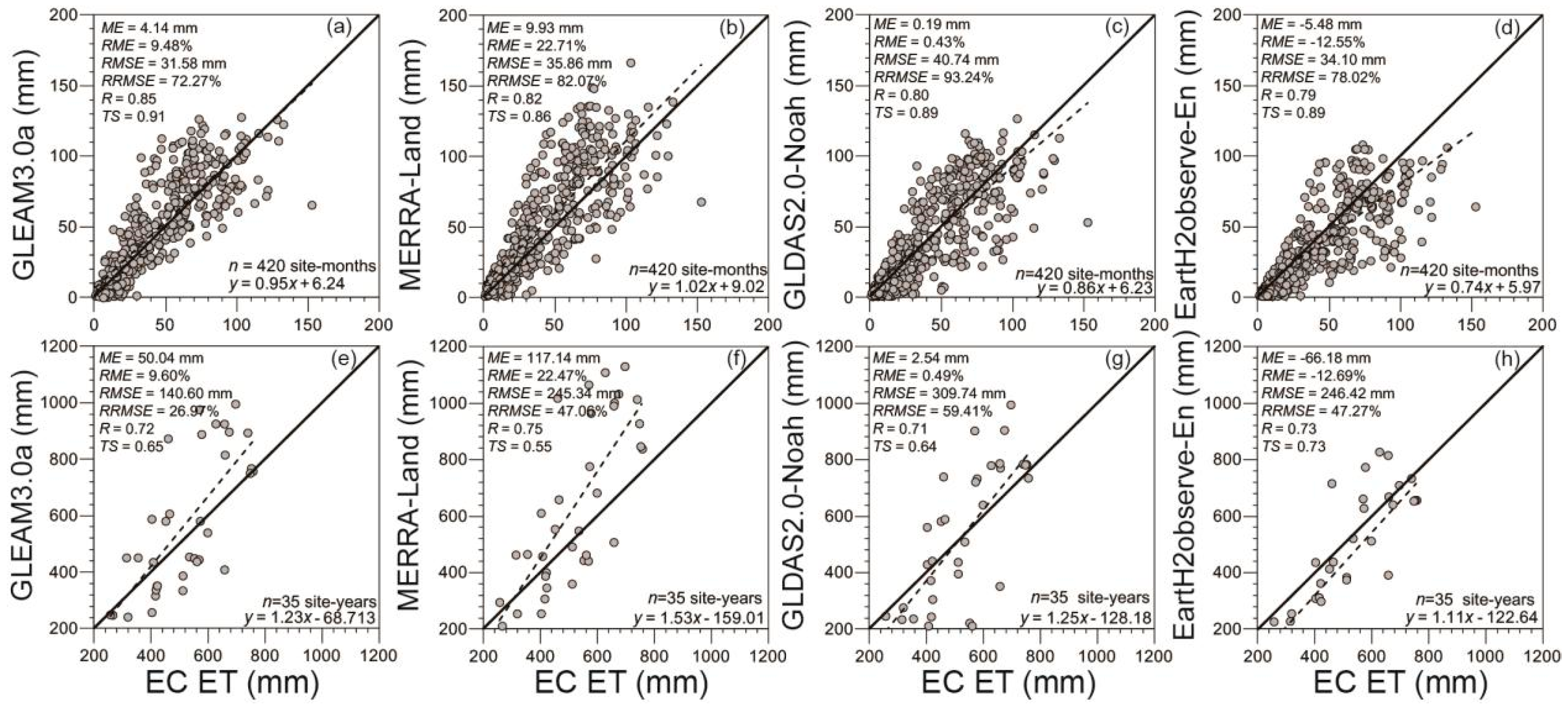
3.1. Validation by the Whole of All of the EC Sites

Figure 2a shows the intra-annual fluctuations of ET products and EC observations averaged over all of the sites. Considering the site-averaged monthly EC ET, there exists an evident seasonality, which is characterized by higher values (>40 mm) during April–September, with a peak in July of 83.69 mm. Intuitively, all four products can effectively capture the intra-annual changes, with the maximum in July ranging from 70.88 mm (EartH2Observe-En) to 97.76 mm (MERRA-Land). In Figure 3a–d, scatter-plots of monthly EC ET against the products are shown based on all of the samples (n = 420 site months) from the twelve sites. Except for EartH2Observe-En, the Rs of the other three products are all larger than 0.80, indicating that their monthly ET estimates can effectively reproduce the spatio-temporal variability of ET when taking all of the monthly data points as a whole. The fitted linear regression equations suggest that, except for MERRA-Land, which always overestimates ET, the other products underestimate ET. However, it should be noted that each product (excluding MERRA-Land) performs differently in estimating lower and higher ET values, i.e., lower ranges are overestimated, but higher ranges are underestimated. Moreover, MERRA-Land ET is overestimated for both lower and higher values, implying that there are potential systemic problems within this product. To further quantify product performance, various validation metrics were calculated against the EC data for the 420 site months; results are presented in the top left corner of each panel of Figure 3a–d. Evidently, MEs (RMEs) differ among these products, ranging between −5.48 mm (−12.55%) for EartH2Observe-En and 9.93 mm (22.71%) for MERRA-Land, which are closely related to their different performances in lower and higher ETs. For example, the negative ME of EartH2Observe-En is mainly because of its underestimates in higher ET (Figure 3d), while the highest and the moderate ME (RME) for MERRA-Land and GLEAM3.0a are closely associated with systemic biases (i.e., overestimates in both lower and higher ETs) and overestimates in lower ET, respectively (Figure 3a,b). Regarding the lowest ME (RME) of GLDAS2.0-Noah, it may be attributed to the bias offset (i.e., overestimates and underestimates in lower and higher ETs, respectively; Figure 3c). Relative to ME (RME) for each product, the RMSE (RRMSE) is much larger; this may be due to both random errors plus different signs in biases, which can introduce additional randomness by aggregating EC sites from various ecosystems. Interestingly, despite the smallest ME (RME), GLDAS2.0-Noah RMSE (RRMSE) is the largest (40.74 mm; 93.24%). Based on TS, the worst, the moderate, and the best overall performances in estimating monthly ET were found to correspond to the MERRA-Land, GLDAS2.0-Noah and EartH2Observe-En, and GLEAM3.0a products, respectively. On an annual scale (Figure 3e–h), lower (higher) values are underestimated (overestimated) in GLEAM3.0a, MERRA-Land, and GLDAS2.0-Noah, whereas EartH2Observe-En always tends to underestimate ET. The bias and error metrics indicate that the rankings of annual performances of the ET products (Figure 3e–h) are consistent with those on the monthly scale (Figure 3a–d). The lowest absolute value of ME (RME) exists in GLDAS2.0-Noah, but GLEAM3.0a has the minimum value of RMSE (RRMSE). In addition, MERRA-Land outperforms the other datasets in terms of annual R, which is in contrast to the largest R in GLEAM3.0a on the monthly scale. This may result from the aggregation of monthly ET into annual values. Regarding the overall performance on the annual scale, EartH2Observe-En and MERRA-Land, respectively, correspond to the maximum and the minimum TS values.

As noted from the scatter-plots of ET products versus EC observation (not shown) and quantitative validation indicators at each month (Figure 4), intra-annual differences in the ET estimation performances are obvious among the four products. Within one year, MEs (in Figure 4a; RMEs in Figure 4b) for MERRA-Land are always positive, corresponding to larger biases during July–October (January–March and September–November). By contrast, EartH2Observe-En shows negative MEs (RMEs) for each month, and larger biases occur during May–August (May–August and November–January). Signs of ME or RME for the other two products vary among months, e.g., a negative ME or RME of GLEAM3.0a (GLDAS2.0-Noah) in January, November, and December (March–July) suggests underestimated ET in these months, while overestimated ET is found in the remaining months. Additionally, based on the magnitudes of ME (RME), GLEAM3.0a has larger values during March–May (February–May and December), but larger values for GLDAS2.0-Noah occur in March–May and September–December (March, April and October–January). Comparing the magnitude of monthly ME (RME) for each product, the maximum bias always occurs in MERRA-Land, excluding March–June and December; however, the ET product with the minimum bias changes among months. As shown in Figure 4c, the monthly RMSE for each ET product is above 10 mm, particularly in April–October, with a value larger than 20 mm. Except for January and December (June–September), MERRA-Land (EartH2Observe-En) always corresponds to the largest (lowest) RMSE. Due to the differences in ET magnitudes among months, intra-annual variation of RRMSE for each product differs from that of RMSE, mainly characterized by larger values in January–May and October–December (Figure 4d); the largest and the lowest RRMSEs in most months occur in MERRA-Land and EartH2Observe-En, respectively. Regarding the R for each product, it sharply declines from January and reaches the minimum (<0.25) in June, but increases rapidly from August (Figure 4e). Overall, all of the products have a higher R during January–April and September–December, and particularly in February and October with the largest value (>0.80). In January–July, GLDAS2.0-Noah (excluding January and May) and EartH2Observe-En (excluding March), respectively, correspond to the maximum and minimum R. By contrast, the smallest (largest) R during August–October exists in GLDAS2.0-Noah (MERRA-Land), and R in November and December is the largest in EartH2Observe-En, but the smallest in MERRA-Land. In Figure 4f, the monthly TS is above 0.50 for all of the products, particularly for January–May and September–December, which are generally higher than 0.70. In January–May and September–December, there are larger differences in TS among the products, and the maximum (~0.90) and the minimum (<0.80) are found in EartH2Observe-En (excluding April in GLDAS2.0-Noah) and MERRA-Land (excluding January in GLDAS2.0-Noah), respectively.

3.2. Validation by Biome

The intra-annual ET variations of all biome types are illustrated in Figure 2b–g. Based on EC ET, characteristics of intra-annual fluctuations suggest apparent differences for the six biome types, i.e., two peaks for MF in June and August (Figure 2b), EBF in July and September (Figure 2d), and CRO in May and August (Figure 2e), with one for the other three biomes in July (Figure 2c,f,g). In spite of some differences in ET magnitude, intra-annual ET fluctuation can be well captured by each product for ENF (Figure 2c), CRO (Figure 2e), GRA (Figure 2f), and WET (Figure 2g); however, for MF (Figure 2b; EBF, Figure 2d), GLEAM3.0a and MERRA-Land (products excluding EartH2Observe-En) cannot reproduce the two ET peaks. With the exception of GLDAS2.0-Noah (EartH2Observe-En), which overestimates lower but underestimates higher ETs for ENF [Figure 5(b3); MF (Figure 5(a4)) and ENF (Figure 5(b4))], all of the ET products were generally overestimated for MF (Figure 5(a1–3)), ENF (Figure 5(b1–2)), and EBF (Figure 5(c1–4)). In CRO, GLEAM3.0a near-perfectly estimated ET (Figure 5(d1)), while MERRA-Land ET was generally overestimated (Figure 5(d2)); relative to the EC measurement, both estimates from the other two products were larger and smaller in lower and higher ETs, respectively (Figure 5(d3–4)). As depicted in Figure 5(e1–4) for GRA and Figure 5(f1–4) for WET, ETs were underestimated by all of the products, especially for WET ET estimates from GLDAS2.0-NOAH and EartH2Observe.

Quantitative validation results for different biome types are shown in the top left corner of each panel of Figure 5. With the exception of Earth2Observe-En with smaller negative ME (RME) in MF, the bias indicators for the other three products are close to or above 10 mm (30%; Figure 5(a1–4)). Correspondingly, Earth2Observe-En RMSE (RRMSE) is the smallest, but the remaining products present a comparable error. Based on R (TS), the ET products show no evident differences in performance, with a value of 0.97 (0.95). As for ENF (Figure 5(b1–4)) and EBF (Figure 5(c1–4)), larger differences in ME (RME) and RMSE (RRMSE) were observed among these products, respectively, corresponding to a range of 7.39–34.76 mm (14.35–65.96%) and 17.72–41.38 mm (34.40–78.52%). Moreover, the maximum for these four metrics always appeared in MERRA-Land, followed by GLEAM3.0a. Despite that, R (TS) in ENF is nearly equal and above 0.85 among these products, and this indicator in EBF is larger than 0.70, except for EartH2Observe-En (MERRA-Land). For CRO (Figure 5(d1–4)), ME (RME) for the ET estimates is different in sign and magnitude (i.e., underestimation for GLEAM3.0a and EartH2Observe-En versus overestimation for MERRA-Land and GLDAS2.0-Noah, and a larger magnitude in MERRA-Land and EartH2Observe-En versus a smaller magnitude in GLEAM3.0a and GLDAS2.0-Noah). In contrast, excluding GLEAM3.0a with a lower RMSE (RRMSE), the performances of the other three products are comparable based on these error indicators (~19 mm; ~34%). Regarding R, the largest value is in GLEAM3.0a, and the next largest is in MERRA-Land, but the other two products have the smallest R. For TS, each product corresponds to a value of approximately 0.90. In GRA (Figure 5(e1–4)) and WET (Figure 5(f1–4)), MEs (RMEs) for all of the products are below zero, accompanied by larger magnitudes for GRA and WET in GLDAS2.0-Noah and EartH2Observe-En. Consistently, GLDAS2.0-Noah and EartH2Observe-En, and GLEAM3.0a and MERRA-Land show larger and smaller errors for both GRA and WET, respectively. R for each product is above 0.83 in GRA (0.92 in WET), of which the minimum is found in GLDAS2.0-Noah. While all products perform differently with respect to the aforementioned five metrics for GRA, they have a comparable TS value of around 0.90. In WET, there is a larger TS range between 0.42 in EartH2Observe-En, and 0.96 in GLEAM3.0a.

3.3. Validation by Elevation Level

Validation results by elevation level (Figure 6) indicate that elevation has an influence on the performance of each ET product. For GLEAM3.0a and MERRA-Land, ET over sites below 1500 m is consistently overestimated (Figure 6(a1–2,b1–2)), while there are different overestimations and underestimations for lower and higher ETs at sites above 1500 m, respectively (Figure 6(c1–2)). For GLDAS2.0-Noah (Figure 6(a3,b3,c3)), overestimated ET is found in the two elevation levels below 500 m (except for some data points with higher ET) and between 500–1500 m; however, evident and systematic underestimations appear at elevations higher than 1500 m. Lower and higher ETs are, respectively, overestimated and underestimated by earth2Observe-En at a low elevation level (Figure 6(a4)), while the other two zones show underestimated ET (Figure 6(b4,c4)), especially for elevation levels above 1500 m.

At elevation levels below 500 m (Figure 6(a1–4)), the MEs (RMEs) of all of the ET datasets are positive, with a range between 0.52 mm (1.05%) in EartH2Observe-En and 13.99 mm (28.32%) in MERRA-Land. Comparing RMSEs (RRMSEs) of the four ET products, MERRA-Land corresponds to the largest value, while the other datasets have more similar values. Regarding R (TS), each product has a value above 0.80, in particular for GLEAM3.0a and GLDAS2.0-Noah (GLDAS2.0-Noah and EartH2Observe-En), which have values higher than 0.84 (0.90). Across the sites with an elevation of 500–1500 m (Figure 6(b1–4)), except for EartH2Observe-En with a slight negative ME (RME), the ET biases of the other datasets are positive and maximized in MERRA-Land. Correspondingly, the largest RMSE (RRMSE) is found in MERRA-Land, followed by the minimum value in EartH2Observe-En. Regarding R (TS), ET products with values near 0.86 (higher than 0.83) perform similarly; moreover, the maximum TS (0.93) occurs in EartH2Observe-En. Unlike the performance based on ME (RME) at the sites below 1500 m, all of the products have a negative bias for high elevation levels (Figure 6(c1–4)); in addition, both GLDAS2.0-Noah and EartH2Observe-En show larger magnitudes, corresponding to the larger RMSE (Figure 6(b3–4)). In spite of some differences in the bias and error metrics, these datasets have an approximate R of 0.87. Comparing TS values, the maximum values (~0.90) are in GLEAM3.0a and MERRA-Land, followed by the moderate (0.76) and the minimum (0.62) values in GLDAS2.0-Noah and EartH2Observe-En, respectively.

3.4. Validation by Climate Regime

The performance of each ET product varies in different climate regimes, i.e., systematic overestimations and underestimations in the wet (except for EartH2Observe-En, with overestimations and underestimations in lower and higher ETs, respectively) and the dry climate regimes, respectively (Figure 7). In the wet climate regime (Figure 7(a1–4)), the maximum ME (RME) of 25.19 mm (48.87%) occurs in MERRA-Land, while the smallest value of 3.11 mm (6.02%) exists in EartH2Observe-En. Of all four datasets, GLEAM3.0a and MERRA-Land exhibit a larger RMSE (RRMSE), while GLDAS2.0-Noah and EartH2Observe correspond to a smaller value. The R values indicate comparable performance among the ET products. Except for MERRA-Land, with the minimum TS of 0.86, the remaining products show a comparable TS of higher than 0.90. For the dry climate regime (Figure 7(b1–4)), MERRA-Land and EartH2Observe-En correspond to the largest and the smallest magnitudes of MEs (RMEs), respectively. For GLDAS2.0-Noah and EartH2Observe-En, RMSEs (RRMSEs) are larger and close to each other, however, the other two datasets have smaller and approximate errors. The performance in R (TS) obviously differs among these ET products (i.e., Rs (TS values) for GLEAM3.0a and MERRA-Land larger than 0.85 (0.90), but those for the other products are near 0.78 (smaller than 0.90)).

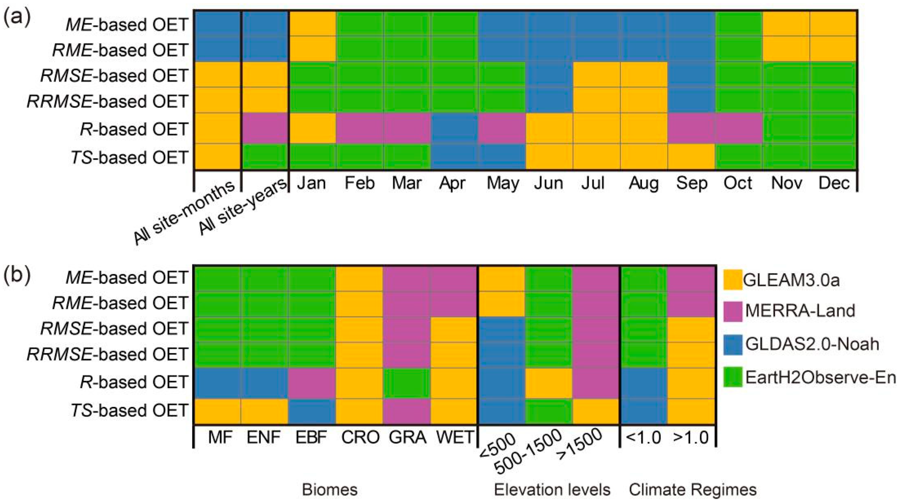
3.5. Optimal ET Products

By comparing the magnitudes of each validation criterion among the four ET products, OET was identified for all 12 EC sites, biomes, elevation levels, and climate regimes (Figure 8). Taking all of the EC sites as a whole (Figure 8a), monthly OETs were GLDAS2.0-Noah (GLEAM3.0a) in view of ME/RME (other four criteria); however, annual OETs vary among these criteria (i.e., GLDAS2.0-Noah, GLEAM3.0a, MERRA-Land, and EartH2Observe-En based on ME/RME, RMSE/RRMSE, R, and TS, respectively). For all 12 months, the ME/RME-based OETs were GLEAM3.0a during January, November, and December; EartH2Observe-En in February–April and October; and GLDAS2.0-Noah from May to September, while EartH2Observe-En as the RMSE/RRMSE-based OET occurred in most months (January–May and October–December). In addition, most months show the R-based OETs of MERRA-Land (February, March, May, September, and October) and GLEAM3.0a (January and June and August), and the TS-based OETs of EartH2Observe-En (January–March and October–December) and GLEAM3.0a (June–September). As illustrated in Figure 8b, EartH2Observe-En were the ME/RMSE- and RMSE/RRMSE-based OETs for the forest biomes (i.e., MF, ENF, and EBF), while the R-based (TS-based) OETs were found to be GLADAS2.0-Noah (GLEAM2.0a) for MF and ENF and MERRA-Land (GLADAS2.0-Noah) for EBF. CRO and WET OETs (excluding the ME/RME-based OET of MERRA-Land) were found in GLEAM3.0a, based on all the validation criteria. Except for EartH2Observe-En (the R-based OET), GRA always had the OET for MERRA-Land for each validation criterion. Figure 8b shows that, given the six criteria, the performances of GLDAS2.0-Noah, EartH2Observe-En, and MERRA-Land were identified as OETs at low, moderate, and high elevation levels, respectively. Over the wet climate regime (Figure 8b), EartH2Observe-En (GLDAS2.0-Noah) was the OET with the smallest ME/RME and RMSE/RRMSE (the highest R and TS), but the dry climate regime had the ME/RME-based OET of MERRA-Land and the RMSE/RRMSE-, R-, and TS-based OET of GLEAM3.0a.

The results noted above show that the performances of each ET product and the corresponding OET differ among classifications of each stratification and among criteria for a certain stratification classification. The differences may be caused by uncertainties of ET products due to simplifications, incomplete hypotheses of model structures and parameterizations, inaccurate models inputs, and uncertainties from the reference ET (i.e., EC ET). We will, therefore, discuss the potential causes of this in the next section.

4. Discussion

4.1. Sources of Uncertainties in ET Products

In the present study, we comprehensively compared and evaluated GLEAM3.0a, MERRA-Land, GLDAS2.0-Noah, and EartH2Observe-En ET products over China based on the EC measurements at twelve sites. From the perspective of all the EC sites, biome, elevation level, and climate regime, the performance of these products varies. Various hypotheses and simplifications of the ET processes, which control the land-atmosphere flux exchanges (e.g., water and energy), have been conducted for each model. Diversities in the complexity of both model structures and parameterizations among models are closely associated with specific applications and/or purposes. Moreover, a variety of inputs are required to run ET models; however, owing to specific requirements for each model and the availability of inputs, the number, types, and/or sources of inputs differ among models. Therefore, we would like to present possible explanations of uncertainties of the ET products from the perspectives of model structures and parameterizations and inputs [4,5,77,78,79,80].

4.1.1. Model Structures and Parameterizations

As shown in Table 1, different PET schemes for estimating ET are employed among the selected models. Thus, the behaviors of the ET products are likely to be directly related to differences in these schemes, which commonly have different levels of capability for capturing PET magnitude and variability given various structural complexities and parameterizations. Regarding the Penman-Monteith scheme, which has been widely regarded as a physically-based expression [71,81], a critical assumption and simplification is that the surface is a “big leaf”, and thus, r_v (aerodynamic resistance to water transfer from the surface to the atmosphere) can be separated into r_c (canopy resistance) and r_h (aerodynamic resistance to heat transfer from the surface to the atmosphere). Even so, to directly run this equation is difficult because of a lack of observed relevant parameters (vegetation–specific parameters, e.g., r_c [82]). Therefore, many diagnostic and physiological equations were proposed based on environmental and biological controls (e.g., vapor pressure deficit, T, solar radiation incident on canopy, and SM) and then was used to estimate these parameters among different biomes [83,84,85]. As for the Priestley-Taylor scheme, it is a simplified variant of the Penman-Monteith equation, in which PET is linearly expressed as a so-called Priestley-Taylor parameter (i.e., α) multiplied by energy available to evaporate water [32]. Generally, the α parameter is between 1.2–1.3 under water unstressed conditions, but it can vary from 1.0 to 1.5; this value is mainly dependent on the degree of coupling between ET processes and the atmosphere, which can be reflected by W, vapor pressure deficit, and SM [4,32]. Komatsu [86] stated that to obtain this parameter, detailed information on canopy and micrometeorological conditions was required, but this knowledge could not be directly supplied, particularly for a larger spatial extent. For this reason alone, α is often set as 1.26 for some widely-used models, while its values of 1.26 in both short vegetation and bare soil fractions and 0.8 for the tall fraction are given by GLEAM3.0a [21,22]. In brief, both the Penman-Monteith and Priestley-Taylor PET schemes differ in their simplifications of some critical parameters, thus resulting in uncertainties and different performances for various ET datasets.

After employing the specified PET scheme for a model, it is vital to calculate the ET fractions from soil and interception evaporation and transpiration, which are summed to estimate ET. Generally speaking, their fractions are parameterized to be jointly controlled by various environmental factors, such as soil properties, SM, vapor pressure deficit, and vegetation parameters (e.g., Leaf Area Index, LAI, and Normalized Difference Vegetation Index, NDVI), and vary greatly among models due to differences and uncertainties of model parameterizations and a lack of observation-based constraints [4]. Taking transpiration (the largest overall contributor to terrestrial ET; [87,88]) as an example, Jasechko et al. [89] pointed out that 90% of terrestrial ET was cycled via vegetation transpiration based on isotope techniques. However, conclusions from Miralles et al. [90] stated that the ratio of transpiration to terrestrial ET from the GLEAM3.0a product was 76% for the whole landmass. This implies that fractions of transpiration have larger discrepancies among models, which possibly propagate into the ET products; the same applies for the ratio of soil or interception evaporation, despite the values being generally smaller [90]. It is particularly noteworthy that even the estimated interception precipitation from the most popular applied approach of the Gash analytical model may produce substantial errors, e.g., an annual overestimation of 39.8 mm in a subtropical evergreen forest of Central-South China [91]; thus, this causes considerable uncertainties in interception evaporation. Therefore, if inaccurate and even incorrect functions for constraining each ET component are used by the models, questionable ET may be provided [4].

As an aside, errors within the estimated ET originate from the neglect of some components of ET, such as night transpiration [92,93]. Based on the assumption that plant stomata is closed at night, and thus transpiration stops, night ET can commonly be ignored for the terrestrial ecosystem; but recent observations have provided evidence that night transpiration is of significance across a wide range of biomes and climate regimes [92,93,94,95,96,97]. For example, Novick et al. [92] reviewed previous studies and pointed out that the percentage of night transpiration accounting for the daily total was basically 10–30%; however, this varied among plant functional groups (i.e., C3 and C4; [93]) and SM conditions [94]. Despite there being no agreement on the mechanisms of night transpiration, it is generally believed that the processes are closely related to W, vapor deficit, SM, and circadian regulation of stomatal conductance [93,97]. Hence, models with no or insufficient considerations of night transpiration processes may lead to systematically underestimated ET.

4.1.2. Model Inputs

If a given ET model is ideally full-biophysical and, thus, can comprehensively describe the ET processes, errors in the ET estimates and differences among the ET products are mainly dependent on various inputs, especially for precipitation and radiation [36,54,60,75,76,79]. Studies have been extensively performed to evaluate different precipitation products (e.g., gauge-based, and reanalysis and remote sensing-related datasets) over the globe [98,99,100,101,102]. For example, Nair and Indu [99] noted that the MSWEP products (input for GLEAM3.0a) in India showed large errors in higher precipitation (i.e., >75th and >95th quantiles), which was confirmed by Alijanian et al. [98] in Iran. Sun et al. [102] found that the CPC-U precipitation (input for MERRA-Land) averaged over the world was underestimated for each season and correspondingly led to the annual value being the smallest compared to other datasets. Moreover, because of relatively limited gauge observations, the CPC-U dataset has overall potential to smooth the precipitation structure and miss local heavy precipitation events [103]. Based on gauge data over the Adige Basin of Italy, the PUMFD precipitation (used by GLDAS2.0-Noah) was assessed by Duan et al. [104], and the conclusions showed that the performance of this precipitation product was the worst relative to others, with biases in the occurrence frequency of daily precipitation for some intensity ranges and higher errors in winter. By comparing different daily precipitation products over Canada, Wong et al. [105] suggested that the skills of the WFDEI (used by EartH2Observe-En) dataset differed from region to region, with underestimation in the northern and eastern parts and overestimation in the west. As shown in Table 1, net radiation used by the four ET models came from different datasets, including ERA-Interim, MERRA version 1.0, PUMFD, and WFDEI for GLEAM3.0a, MERRA-Land, GLDAS2.0-Noah, and EartH2Observe-En, respectively. With respect to the radiation datasets, assessments have been conducted across the world [4,66,79,106,107,108,109,110,111,112]. In Boilly and Wald [109], ERA-Interim radiation was overestimated overall to some degree in Europe, Africa, and the Atlantic Ocean, whereas clear and cloudy sky conditions, respectively, corresponded to overestimation and underestimation. Regarding MERRA version 1.0, it showed significantly overestimated net radiation at the twenty-three EC sites and aggregated over the whole of China; moreover, the net radiation was almost 2.8 times the Global Energy and Water Exchanges (GEWEX) value [79], which might be caused by the overestimation of the occurrence of clear sky conditions [107,109]. Tory and Wood [106] compared and evaluated gridded radiation products across northern Eurasia and found that there were smaller biases for the PUMFD dataset on an annual scale, but larger errors on a seasonal scale. For the WFDEI dataset, the downwelling shortwave radiation is higher in northern Africa but lower in northern South America, despite the effects of interannual changes in the atmospheric aerosol optical depths being considered [110]; thus, net radiation would be overestimated. Apart from precipitation and radiation, other meteorological forcings (e.g., T, W, Q, and SP) are also different for MERRA-Land, GLDAS2.0-Noah, and EartH2Observe-En (Table 1), integrated with different accuracies [6,26,66]. These studies indicated evident discrepancies among the existing meteorological datasets in both magnitude and variability on daily to annual scales (e.g., owing to the number and spatial coverage of surface stations, satellite algorithms, and data assimilation systems); meanwhile, their capabilities to capture meteorological conditions differed from region to region.

It is well known that descriptions of vegetation processes, definitions of land use/cover (LUC) and relevant vegetation character parameters (e.g., NDVI, LAI, and/or VOD) are needed; thus, their differences and uncertainties potentially propagate into the ET estimates [113]. There are a number of available LUC (e.g., Table S3) and NDVI/LAI/VOD products derived from different data sources (e.g., various satellite images), algorithms, and classification schemes [114,115]. It should be noted, however, that these datasets were produced for specific purposes and applications, including analyses of LUC and vegetation changes and their impacts on the climate, hydrology, and ecosystem, and the developments of various geo-scientific models; thus, obvious discrepancies and even errors in these products have been reported, especially at the regional scale [115,116,117,118,119,120,121,122,123,124,125]. Therefore, without considering the suitability of LUC and NDVI/LAI/VOD products, biases originating from raw data and inconsistencies among the selected products and uncertainties owing to product selection and processing can be of the same magnitude as those from the representation of the processes under investigation [113,121,126,127,128,129]. For example, Branger et al. [126] investigated the impact of different LUC datasets on the long-term water balance of the Yzeron peri-urban catchment of France and stated that most water quantities (including ET) were sensitive to LUC selections. Liu et al. [113] quantified uncertainties of simulated water fluxes using MODIS (MOD15), GLASS, and the Four-Scale Geometric Optical Model (FSGOM)-based LAI, and concluded that LAI products could lead to substantial uncertainties in the ET estimates. For these selected ET products, different LUCs and vegetation character parameters are used and cause differences in performances and uncertainties of the ET estimates.

4.2. Uncertainties of EC ET

Since the EC technique was first applied [130], it has been used extensively to directly measure terrestrial carbon, water, and energy cycles, and taken as ground truth values for evaluating various ET products [4,131]. Nevertheless, there are still uncertainties regarding EC observations. Especially problematic is energy imbalance at EC sites, mainly characterized by the energy closure ratio (i.e., the sum of observed latent and sensible heat divided by the difference of net radiation and ground heat flux), not being equal to one [132]. Based on numerous previous conclusions, energy balance non-closure can generally be attributed to the missed very low and/or high-frequency fluctuations of fluxes, measurement errors associated with sensor separation, interference from tower or instrument-mounting structures, not fully considering the storage term (e.g., canopy and photosynthesis storage), mismatch between the scales of energy balance components, large-eddy transport, or secondary circulations not captured by the EC technique [37,133]. It is reported that, in general, the sum of observed latent and sensible heat is 10–30% smaller than the difference between net radiation and ground heat flux at EC sites [32,132]; moreover, the closure error can vary seasonally and inter-annually and from biome to biome [32,133,134,135]. Scholars have often suggested that underestimation of latent heat has largely contributed to this energy non-closure of the EC technique [136,137,138]. For instance, Finkelstein and Sims [136] indicated that the normalized errors for sensible and latent heat were 10% and 25–30%, respectively.

In addition, the spatial context of the EC measurement is limited and defined within the footprint of a turbulent flux measurement [131,139]. For a deployed turbulent flux sensor, its detected signals reflect influences of the underlying surface on the turbulent exchange. Over a homogeneous surface with enough spatial extent (i.e., at least ~1 km; [111]), the measured fluxes from all parts of the surface are, by definition, equal. However, the surface is typically inhomogeneous; the EC measurement is dependent on which part of the surface exerts the strongest impact on the sensor and consequently on the location and size of its footprint [139]. To reduce the influence from the inhomogeneous surface and, thus, enhance the spatial representation, many footprint models have been developed and used to identify and parameterize the footprint of each EC site [139,140,141]. Despite that, the measured signals in most cases involve influences from the untargeted surfaces within the footprint, indicating that the observations at the EC site cannot perfectly reflect energy and gas fluxes from the targeted surface. Notably, the spatial extent of the footprint is not unchangeable, but can vary with W and its direction, stability, and measurement heights [4,142,143]; therefore, the fixed parameterization of the footprint can also introduce uncertainties into the EC observations. Besides the energy imbalance and limited spatial representativeness, errors of EC ET can result from missing data post-processing, which are attributed to instrument failure, poor maintenance, instances of bad weather, and data rejection [131].

4.3. Other Factors Influencing Validation Results

In addition to uncertainties from the ET models and the EC observations, impacts from other factors (e.g., spatial scale problems among ET estimates and necessary inputs for running models, and data aggregation) on the validation results should be considered. In this study, the selected four ET products have different spatial resolutions and corresponding spatial extents much larger than the footprint of the EC site. Given the larger grid, greater potential exists for spatial heterogeneity in surface characteristics (e.g., LUC, vegetation parameters, and elevation) and meteorological inputs for estimating ET. The estimated ET value by the models actually reflects the combination of influences from different landscapes rather than any single landscape. By contrast, the EC measurement corresponds to a relatively homogenous footprint (even though it is not perfectly uniform) and represents the ET from a given landscape to a great extent. As a result, not considering impacts from the spatial scale mismatch, conducting a direct comparison between the ET products and the EC measurements is likely to influence the validation results [23,76,144]. To qualitatively compare the impacts of different LUCs, we have collected most (i.e., GLEAM3.0a, MERRA-Land, GLDAS2.0-Noah, and seven models within EartH2Observe-En) of the LUC maps used by these ET products, including MODIS (i.e., MOD12Q1, MCD12Q1, and MOD44B), and the Global Land Cover Characterization (GLCC) Version 2 and GlobCover 2009 v2.3 products, which are produced at different spatial resolutions and classification systems (i.e., IGBP, Simple Biosphere 2 Model, and GlobCover legends). Corresponding LUC types at 12 EC sites are identified (Table S3). As depicted in Figure 8b, GLEAM3.0a ET outperforms other products in each validation criterion. This result may be related to the reasonable treatment on vegetation types at Yc and Sx sites in GLEAM3.0a [i.e., dominant type of low vegetation (e.g., grassland) versus IGBP CRO]. The EC sites with MF, ENF, or EBF correspond to the dominant types of tall vegetation (except for Qyz) in GLEAM3.0a (Table S3). However, based on RME and RRMSE (which can partly remove regional differences), the performance of GLEAM3.0a ET is better than MERRA-Land, with smaller differences among the forest sites. This may be associated with the GLEAM3.0a ET algorithms for tall vegetation. As another example, WET at the Has site is simply specified as low vegetation, agriculture, or C3 grassland, and GRA by the ET products (Table S3). As a result, the ETs are underestimated at this site due to large discrepancies of ET mechanisms between WET and other vegetation types (i.e., generally there are no water limits for evaporation and transpiration in WET). Because of the lack of detailed descriptions of the digital elevation model (DEM) datasets used by some ET models, we would like to discuss the impacts of mismatch in elevation levels from several popular DEM datasets (Table S4) on validation results. Obviously, there is perfect agreement on elevation levels based on grid mean elevations over all the EC sites. However, we found that within the 0.25° × 0.25° grid at the Qyz and Dhs sites, there exists larger spatial variability in elevations for each DEM dataset compared to the corresponding grid mean values (the ratio between mean and spatial variability is less than 2.5); this suggests that the representativeness of the topography at these two sites is lower, and consequently influences the evaluation results at low elevation levels. Generally, we found that elevations from EC metadata have limited impacts on the results at moderate and high elevation levels; however, future studies should examine to what magnitude the higher spatial variability of the elevation at the Qyz and Dhs sites impacts validations at low elevation levels.

To make a comparison and evaluation possible, all of the ET products were aggregated to the same spatial (0.25° × 0.25°) and temporal (monthly) resolutions, and the EC measurements were integrated into monthly values. The aggregations of the ET products and EC ET can impact the comparisons and often reduce the confidence in any subsequent model performance ranking [75,76,145]. Among the ET models, we can find different spatial resolutions for the driving factors, which are dependent on the specified requirements of the ET model. Several studies have examined the impacts of spatial resolutions of inputs on the estimated ET [32,146,147]. McCabe and Wood [147] calculated the ET based on the Surface Energy Balance method and necessary inputs derived from three satellite platforms with different spatial resolutions, and compared the results with the flux tower ET on the Walnut Creek watershed in Iowa. They found that despite the comparable accuracy of the regional mean MODIS-based ET relative to the other two higher resolution estimates, the MODIS-based retrievals could not effectively reproduce the flux tower ET, mainly because the MODIS inputs were unable to discriminate the influence of land surface heterogeneity at field scales. Thus, the influences of the different spatial scales of the inputs for driving models would be reflected in the ET products.

5. Conclusions

In this study, we conduct point-scale evaluations of four ET global products [one remote sensing-based product (GLEAM3.0a), two reanalysis-based product (MERRA-Land and GLDAS2.0-Noah), and one LSM ensemble dataset (EartH2Observe-En)] at 12 EC sites across China, focusing on the bias, error, and overall performance of the datasets, as well as their capabilities in capturing the spatio-temporal variability of ET. The major results are summarized below:

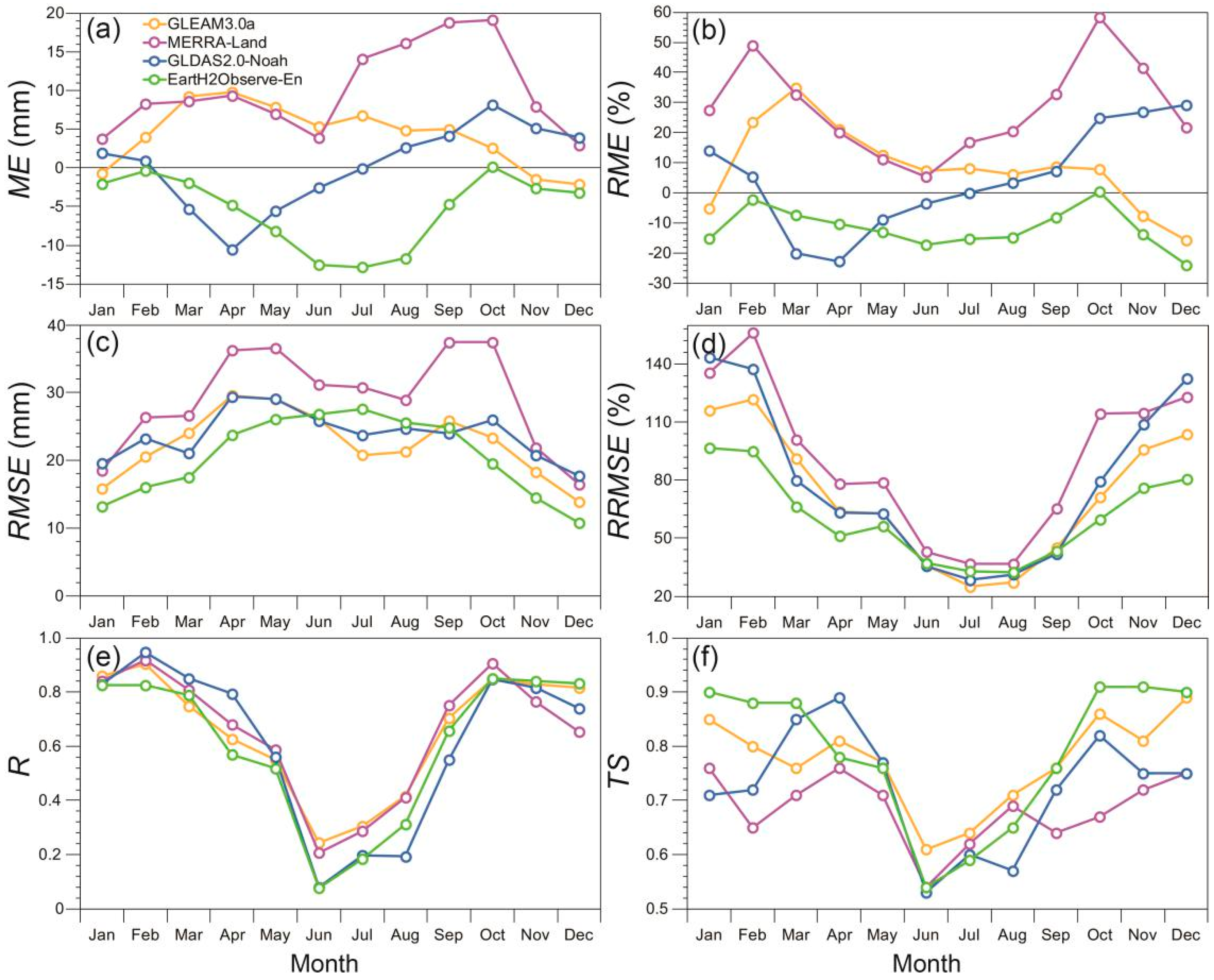
• Validation using all of 12 EC sites: Generally, these products reproduce intra-annual ET fluctuations but perform differently in view of each validation criterion. GLDAS2.0-Noah (GLEAM3.0a) shows minimum monthly biases (annual errors). The highest monthly and annual Rs (TS values) occur in GLEAM3.0a and MERRA-Land (GLEAM3.0a and EartH2Observe-En), respectively. The metrics vary among all 12 months.
• Validation by biome: ETs in MF, ENF, and EBF are generally overestimated, but underestimated in GRA and WET. In CRO, MERRA-Land, and GLDAS2.0a-Noah (remaining two products) overestimate (underestimate) ET. Except for GLEAM3.0a and MERRA-Land in ENF and EBF, and GLDAS2.0-Noah and EartH2Observe-En in WET, a comparable error exists among the six biomes. Relative to EBF, the products in the remaining biomes (excluding GLDAS2.0-Noah and EartH2Observe-En in WET) show higher Rs and TS values.
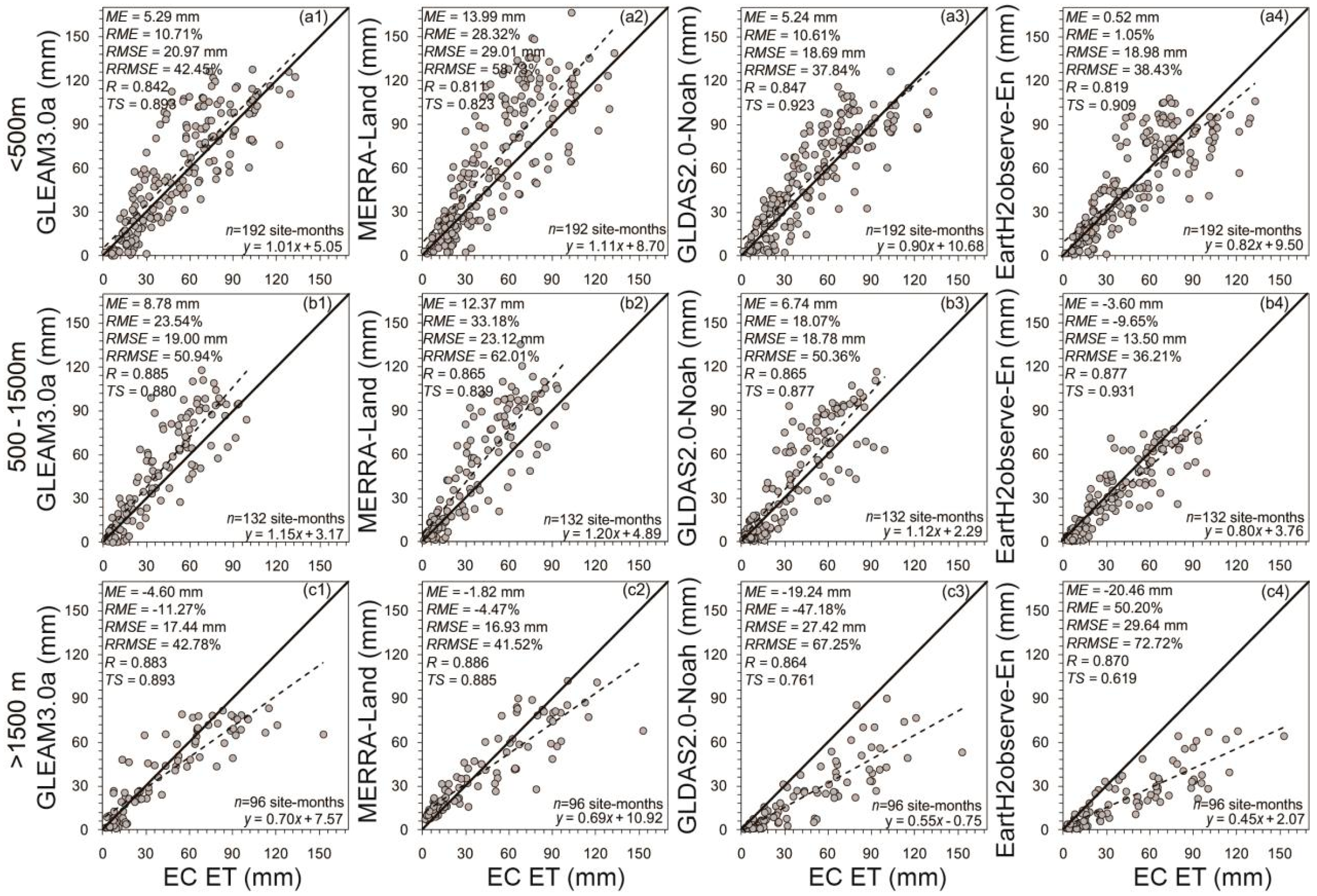
• Validation by elevation level: All products underestimated and overestimated ET, respectively, for high and medium/low elevations (excluding EartH2Observe-En for moderate elevations). Each product showed comparable error, except for the RMES values of MERRA-Land for low and moderate elevations and errors of GLDAS2.0-Noah and EartH2Observe-En for high elevations. Compared to low elevation levels, Rs for medium and high elevation levels were slightly larger. Larger TS values were found in all elevation levels, except for GLDAS2.0-Noah and EartH2Observe-En for high elevation levels.
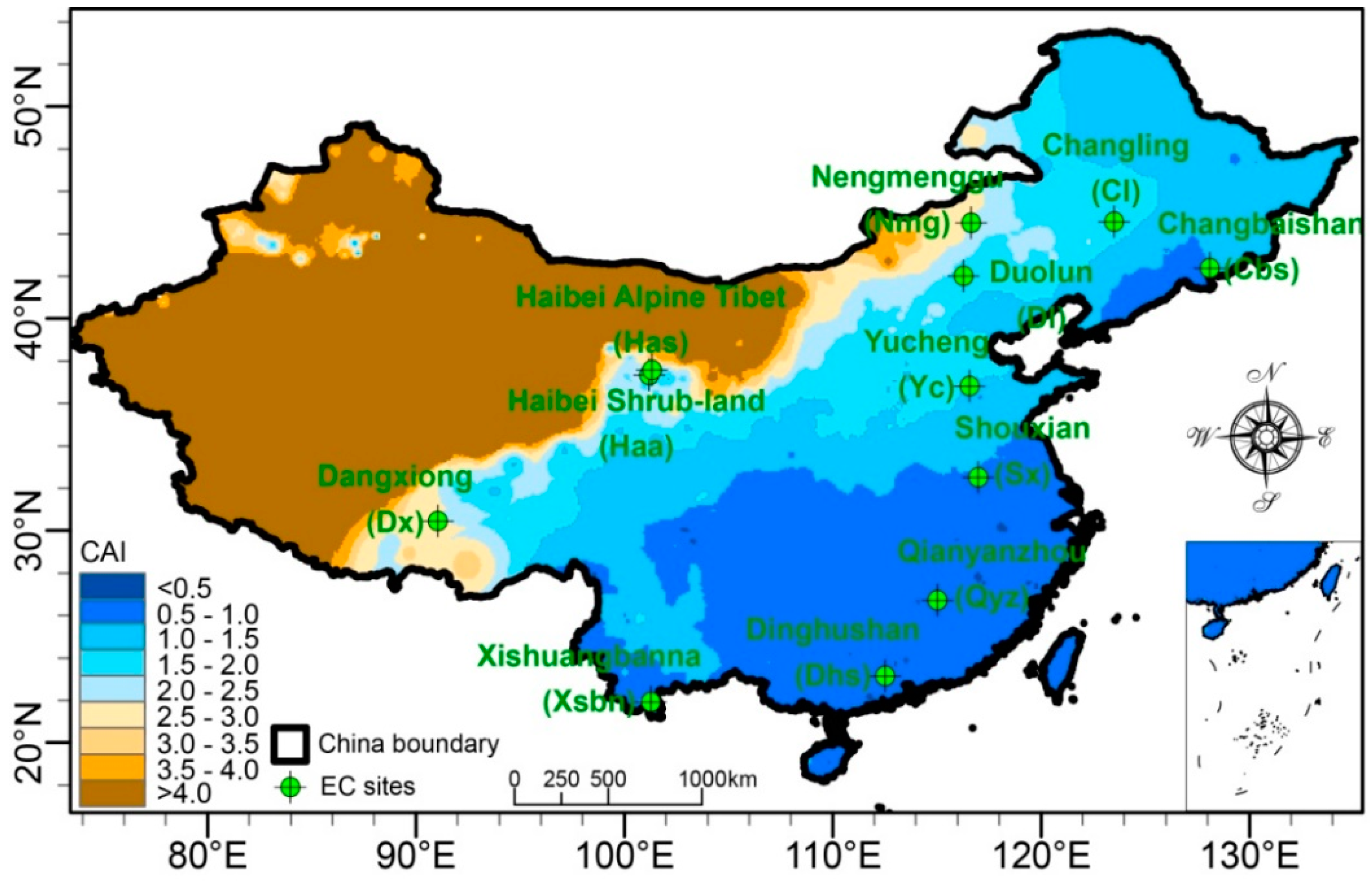
• Validation by climate regime: ETs in wet (dry) regions were always overestimated (underestimated). In wet regions, GLEAM3.0a and MERRA-Land (remaining two products) show larger (smaller) errors, in contrast to dry regions. Excluding GLDAS2.0-Noah and EartH2Observe-En in dry regions (MERRA-Land and EartH2Observe-En in wet and dry regions, respectively), Rs (TS values) are larger for each climate regime.
• OETs: Overall, the OETs varied among stratification classifications (the selected six criteria). In other words, no product always performed best in terms of the validation criteria.

References

1. Wild, M.; Grieser, J.; Schär, C. Combined surface solar brightening and increasing greenhouse effect support recent intensification of the global land-based hydrological cycle. Geophys. Res. Lett. 2008, 35, L17706. [Google Scholar] [CrossRef]
2. Sun, S.L.; Chen, H.S.; Ju, W.M.; Yu, M.; Hua, W.J.; Yin, Y. On the attribution of the changing hydrological cycle in Poyang Lake Basin, China. J. Hydrol. 2014, 514, 214–225. [Google Scholar] [CrossRef]
3. Miralles, D.G.; van den Berg, M.J.; Gash, J.H.; Parinussa, R.M.; De Jeu, R.A.M.; Beck, H.E.; Holmes, T.R.H.; Jiménez, C.; Verhoest, N.E.C.; Dorigo, W.A.; et al. El Niño-La Niña cycle and recent trends in continental evaporation. Nat. Clim. Chang. 2014, 4, 122–126. [Google Scholar] [CrossRef]
4. Wang, K.C.; Dickinson, R.E. A review of global terrestrial evapotranspiration: Observation, modeling, climatology, and climatic variability. Rev. Geophys. 2012, 50, RG2005. [Google Scholar] [CrossRef]
5. Sörensson, A.A.; Ruscica, R.C. Intercomparison and uncertainty assessment of nine evapotranspiration estimates over South America. Water Resour. Res. 2018, 54, 2891–2908. [Google Scholar] [CrossRef]
6. Sheffield, J.; Wood, E.F.; Roderick, M.L. Little change in global drought over the past 60 years. Nature 2012, 491, 435–438. [Google Scholar] [CrossRef] [PubMed]
7. Mueller, B.; Hirschi, M.; Jimenez, C.; Ciais, P.; Dirmeyer, P.A.; Dolman, A.J.; Fisher, J.B.; Jung, M.; Ludwig, F.; Maignan, F.; et al. Benchmark products for land evapotranspiration: LandFlux-EVAL multi-data set synthesis. Hydrol. Earth Syst. Sci. 2013, 17, 3707–3720. [Google Scholar] [CrossRef]
8. Majozi, N.P.; Mannaerts, C.M.; Ramoelo, A.; Mathieu, R.; Mudau, A.E.; Verhoef, W. An intercomparison of satellite-based daily evapotranspiration estimates under different eco-climatic regions in South Africa. Remote Sens. 2017, 9, 307. [Google Scholar] [CrossRef]
9. Sun, S.L.; Chen, H.S.; Ju, W.M.; Wang, G.J.; Sun, G.; Huang, J.; Ma, H.D.; Hua, W.J.; Yan, G.X. On the coupling between precipitation and potential evapotranspiration: Contributions to decadal drought anomalies in the Southwest China. Clim. Dyn. 2017, 48, 3779–3797. [Google Scholar] [CrossRef]
10. Kousari, M.R.; Ahani, H. An investigation on reference crop evapotranspiration trend from 1975 to 2005 in Iran. Int. J. Climatol. 2012, 32, 2387–2402. [Google Scholar] [CrossRef]
11. Andam-Akorful, S.A.; Ferreira, V.G.; Awange, J.L.; Forootan, E.; He, X.F. Multi-model and multi-sensor estimations of evapotranspiration over the Volta Basin, West Africa. Int. J. Climatol. 2015, 35, 3132–3145. [Google Scholar] [CrossRef]
12. Zhang, K.; Kimball, J.S.; Running, S.W. A review of remote sensing based actual evapotranspiration estimation. Wiley Interdiscip. Rev. Water 2016, 3, 834–853. [Google Scholar] [CrossRef]
13. Jian, D.; Li, X.; Sun, H.; Tao, H.; Jiang, T.; Su, B.; Hartmann, H. Estimation of actual evapotranspiration by the complementary theory-based advection-aridity model in the Tarim River Basin, China. J. Hydrometeorol. 2018, 19, 289–303. [Google Scholar] [CrossRef]
14. Allen, R.G.; Howell, T.A.; Pruitt, W.O.; Walter, I.A.; Jensen, M.E. (Eds.) Lysimeters for Evapotranspiration and Environmental Measurements; ASCE Publication: Reston, VA, USA, 1991; p. 444. [Google Scholar]
15. Bowen, I.S. The ratio of heat loss by conduction and by evaporation from any water surface. Phys. Rev. 1926, 27, 779–787. [Google Scholar] [CrossRef]
16. Monteith, J.L.; Unsworth, M.H. Principles of Environmental Physics; Edword Arnold: London, UK, 1990. [Google Scholar]
17. Everson, C.S.; Clulow, A.; Mengitsu, M. Feasibility Study on the Determination of Riparian Evaporation in Non-Perennial Systems; WRC Report No. TT 424/09; Water Research Commission: Pretoria, South Africa, 2009. [Google Scholar]
18. Xu, C.-Y.; Singh, V.P. Evaluation of three complementary relationship evapotranspiration models by water balance approach to estimate actual regional evapotranspiration in different climatic regions. J. Hydrol. 2005, 308, 105–121. [Google Scholar] [CrossRef]
19. Su, Z. The surface energy balance system SEBS for estimation of turbulent heat fluxes. Hydrol. Earth Syst. Sci. 2002, 6, 85–99. [Google Scholar] [CrossRef]
20. Fisher, J.B.; Tu, K.P.; Baldocchi, D.D. Global estimates of the land-atmosphere water flux based on monthly AVHRR and ISLSCP-II data, validated at 16 FLUXNET sites. Remote Sens. Environ. 2008, 112, 901–919. [Google Scholar] [CrossRef]
21. Miralles, D.G.; de Jeu, R.A.M.; Gash, J.H.; Holmes, T.R.H.; Dolman, A.J. Magnitude and variability of land evaporation and its components at the global scale. Hydrol. Earth Syst. Sci. 2011, 15, 967–981. [Google Scholar] [CrossRef] [Green Version]
22. Miralles, D.G.; Holmes, T.R.H.; de Jeu, R.A.M.; Gash, J.H.; Meesters, A.G.C.A.; Dolman, A.J. Global land-surface evaporation estimated from satellite-based observations. Hydrol. Earth Syst. Sci. 2011, 15, 453–469. [Google Scholar] [CrossRef] [Green Version]
23. Mu, Q.; Zhao, M.; Running, S.W. Improvements to a MODIS Global Terrestrial Evapotranspiration Algorithm. Remote Sens. Environ. 2011, 115, 1781–1800. [Google Scholar] [CrossRef]
24. Onogi, K.; Tsutsui, J.; Koide, H.; Sakamoto, M.; Kobayashi, S.; Hatsushika, H.; Matsumoto, T.; Yamazaki, N.; Kamahori, H.; Takahashi, K.; et al. The JRA-25 Reanalysis. J. Meteorol. Soc. Jpn. 2007, 85, 369–432. [Google Scholar] [CrossRef] [Green Version]
25. Dee, D.P.; Uppala, S.M.; Simmons, A.J.; Berrisford, P.; Poli, P.; Kobayashi, S.; Andrae, U.; Balmaseda, M.A.; Balsamo, G.; Bauer, P.; et al. The ERA-Interim reanalysis: Configuration and performance of the data assimilation system. Q. J. R. Meteorol. Soc. 2011, 137, 553–597. [Google Scholar] [CrossRef]
26. Reichle, R.H.; Draper, C.S.; Liu, Q.; Girotto, M.; Mahanama, S.P.P.; Koster, R.D.; de Lannoy, G.J.M. Assessment of MERRA-2 land surface hydrology estimates. J. Clim. 2017, 30, 2937–2960. [Google Scholar] [CrossRef]
27. Bosilovich, M.G.; Robertson, F.R.; Takacs, L.; Molod, A.; Mocko, D. Atmospheric water balance and variability in the MERRA-2 reanalysis. J. Clim. 2017, 30, 1177–1196. [Google Scholar] [CrossRef]
28. Rodell, M.; Houser, P.R.; Jambor, U.; Gottschalck, J.; Mitchell, K.; Meng, C.-J.; Arsenault, K.; Cosgrove, B.; Radakovich, J.; Bosilovich, M.; et al. The global land data assimilation system. Bull. Am. Meteorol. Soc. 2004, 85, 381–394. [Google Scholar] [CrossRef]
29. Haddeland, I.; Clark, D.B.; Franssen, W.; Ludwig, F.; Voß, F.; Arnell, N.W.; Bertrand, N.; Best, M.; Folwell, S.; Gerten, D.; et al. Multimodel estimate of the global terrestrial water balance: Setup and first results. J. Hydrometeorol. 2011, 12, 869–884. [Google Scholar] [CrossRef]
30. Schellekens, J.; Dutra, E.; Martínez-de la Torre, A.; Balsamo, G.; van Dijk, A.; Sperna Weiland, F.; Minvielle, M.; Calvet, J.-C.; Decharme, B.; Eisner, S.; et al. A global water resources ensemble of hydrological models: The eartH2Observe Tier-1 dataset. Earth Syst. Sci. Data 2017, 9, 389–413. [Google Scholar] [CrossRef]
31. Jung, M.; Reichstein, M.; Bondeau, A. Towards global empirical upscaling of FLUXNET eddy covariance observations: Validation of a model tree ensemble approach using a biosphere model. Biogeosciences 2009, 6, 2001–2013. [Google Scholar]
32. Glenn, E.P.; Huete, A.R.; Nagler, P.L.; Hirschboeck, K.K.; Brown, P. Integrating remote sensing and ground methods to estimate evapotranspiration. Crit. Rev. Plant Sci. 2007, 26, 139–168. [Google Scholar] [CrossRef]
33. Kalma, J.D.; McVicar, T.R.; McCabe, M.F. Estimating land surface evaporation: A Review of methods using remotely sensed surface temperature data. Surv. Geophys. 2008, 29, 421–469. [Google Scholar] [CrossRef]
34. Ershadi, A.; McCabe, M.; Evans, J.; Chaney, N.; Wood, E. Multi-site evaluation of terrestrial evaporation models using FLUXNET data. Agric. For. Meteorol. 2014, 187, 46–61. [Google Scholar] [CrossRef]
35. Allen, R.G.; Pereira, L.S.; Howell, T.A.; Jensen, M.E. Evapotranspiration information reporting: I. Factors governing measurement accuracy. Agric. Water Manag. 2011, 98, 899–920. [Google Scholar] [CrossRef]
36. Fisher, J.B.; Melton, F.; Middleton, E.; Hain, C.; Anderson, M.; Allen, R.; McCabe, M.; Hook, S.; Baldocchi, D.; Townsend, P.A.; et al. The Future of Evapotranspiration: Global requirements for ecosystem functioning, carbon and climate feedbacks, agricultural management, and water resources. Water Resour. Res. 2017, 53, 2618–2626. [Google Scholar] [CrossRef]
37. Foken, T. The energy balance closure problem: An overview. Ecol. Appl. 2008, 18, 1351–1367. [Google Scholar] [CrossRef] [PubMed]
38. Kim, H.W.; Hwang, K.; Mu, Q.; Lee, S.O.; Choi, M. Validation of MODIS 16 global terrestrial evapotranspiration products in various climates and land cover types in Asia. KSCE J. Civ. Eng. 2012, 16, 229–238. [Google Scholar] [CrossRef]
39. Zhang, F.; Zhou, G.; Wang, Y.; Yang, F.; Nilsson, C. Evapotranspiration and crop coefficient for a temperate desert steppe ecosystem using eddy covariance in Inner Mongolia, China. Hydrol. Process. 2012, 26, 379–386. [Google Scholar] [CrossRef]
40. Michel, D.; Jiménez, C.; Miralles, D.G.; Jung, M.; Hirschi, M.; Ershadi, A.; Martens, B.; McCabe, M.F.; Fisher, J.B.; Mu, Q.; et al. The WACMOS-ET project-Part 1: Tower-scale evaluation of four remote-sensing-based evapotranspiration algorithms. Hydrol. Earth Syst. Sci. 2016, 20, 803–822. [Google Scholar] [CrossRef] [Green Version]
41. Numata, I.; Khand, K.; Kjaersgaard, J.; Cochrance, M.; Silva, S. Evaluation of Landsat-based METRIC modeling to provide high-spatial resolution evapotranspiration estimates for Amazonian forests. Remote Sens. 2017, 9, 46. [Google Scholar] [CrossRef]
42. Yang, X.; Yong, B.; Ren, L.; Zhang, Y.; Long, D. Multi-scale validation of GLEAM evapotranspiration products over China via ChinaFLUX ET measurements. Int. J. Remote Sens. 2017, 38, 5688–5709. [Google Scholar] [CrossRef]
43. Fu, G.; Yu, J.; Zhang, Y.; Hu, S.; Ouyang, R.; Liu, W. Temporal variation of wind speed in China for 1961–2007. Theor. Appl. Climatol. 2010, 104, 313–324. [Google Scholar] [CrossRef] [Green Version]
44. Xie, B.; Zhang, Q.; Ying, Y. Trends in precipitable water and relative humidity in China: 1979–2005. J. Clim. 2011, 50, 1985–1994. [Google Scholar] [CrossRef]
45. Huang, J.; Sun, S.; Xue, Y.; Li, J.; Zhang, J. Spatial and temporal variability of precipitation and dryness/wetness during 1961–2008 in Sichuan Province, West China. Water Resour. Manag. 2014, 28, 1655–1670. [Google Scholar] [CrossRef]
46. Huang, J.; Sun, S.; Xue, Y.; Zhang, J. Changing characteristics of precipitation during 1960–2012 in Inner Mongolia, northern China. Meteorol. Atmos. Phys. 2015, 127, 257–271. [Google Scholar] [CrossRef]
47. Huang, J.; Sun, S.; Zhang, J. Detection of trends in precipitation during 1960–2008 in Jiangxi province, southeast China. Theor. Appl. Climatol. 2013, 114, 237–251. [Google Scholar] [CrossRef]
48. Liao, W.; Wang, X.; Fan, Q.; Zhou, S.; Chang, M.; Wang, Z.; Wang, Y.; Tu, Q. Long-term atmospheric visibility, sunshine duration and precipitation trends in South China. Atmos. Environ. 2015, 107, 204–216. [Google Scholar] [CrossRef]
49. Wang, K.C.; Ma, Q.; Li, Z.; Wang, J. Decadal variability of surface incident solar radiation over China: Observations, satellite retrievals, and reanalyses. J. Geophys. Res. 2015, 120, 6500–6514. [Google Scholar] [CrossRef] [Green Version]
50. Cao, L.; Yan, Z.; Zhao, P.; Zhu, Y.; Yu, Y.; Tang, G.; Jones, P. Climatic warming in China during 1901–2015 based on an extended dataset of instrumental temperature records. Environ. Res. Lett. 2017, 12, 064005. [Google Scholar] [CrossRef]
51. Feng, F.; Wang, K. Merging satellite retrievals and reanalyses to produce global long-term and consistent surface incident solar radiation datasets. Remote Sens. 2018, 10, 115. [Google Scholar] [CrossRef]
52. Schneider, K.; Ketzer, B.; Breuer, L.; Vaché, K.B.; Bernhofer, C.; Frede, H.G. Evaluation of evapotranspiration methods for model validation in a semi-arid watershed in northern China. Adv. Geosci. 2007, 11, 37–42. [Google Scholar] [CrossRef]
53. Xiao, J.; Sun, G.; Chen, J.; Chen, H.; Chen, S.; Dong, G.; Gao, S.; Guo, H.; Guo, J.; Han, S.; et al. Carbon fluxes, evapotranspiration, and water use efficiency of terrestrial ecosystems in China. Agric. For. Meteorol. 2013, 182–183, 76–90. [Google Scholar] [CrossRef]
54. Chen, Y.; Xia, J.; Liang, S.; Feng, J.; Fisher, J.B.; Li, X.; Li, X.; Liu, S.; Ma, Z.; Miyata, A.; et al. Comparison of satellite-based evapotranspiration models over terrestrial ecosystems in China. Remote Sens. Environ. 2014, 140, 279–293. [Google Scholar] [CrossRef]
55. Tang, R.; Shao, K.; Li, Z.L.; Wu, H.; Tang, B.-H.; Zhou, G.; Zhang, L. Multiscale validation of the 8-day MOD16 evapotranspiration product using flux data collected in China. IEEE J. Sel. Top. Appl. Earth Obs. Remote Sens. 2015, 8, 1478–1486. [Google Scholar] [CrossRef]
56. Yang, Y.; Long, D.; Guan, H.; Liang, W.; Simmons, C.; Batelaan, O. Comparison of three dual-source remote sensing evapotranspiration models during the MUSOEXE-12 campaign: Revisit of model physics. Water Resour. Res. 2015, 51, 3145–3165. [Google Scholar] [CrossRef] [Green Version]
57. Zhou, Y.; Li, X.; Yang, K.; Zhou, J. Assessing the impacts of an ecological water diversion project on water consumption through high-resolution estimations of actual evapotranspiration in the downstream regions of the Heihe River Basin, China. Agric. For. Meteorol. 2018, 249, 210–227. [Google Scholar] [CrossRef]
58. Martens, B.; Miralles, D.G.; Lievens, H.; van der Schalie, R.; de Jeu, R.A.M.; Fernández-Prieto, D.; Beck, H.E.; Dorigo, W.A.; Verhoest, N.E.C. GLEAM v3: Satellite-based land evaporation and root-zone soil moisture. Geosci. Model Dev. 2017, 10, 1903–1925. [Google Scholar] [CrossRef]
59. Liu, Y.Y.; de Jeu, R.A.M.; McCabe, M.F.; Evans, J.P.; van Dijk, A.I.J.M. Global long-term passive microwave satellite based retrievals of vegetation optical depth. Geophys. Res. Lett. 2011, 38, L18402. [Google Scholar] [CrossRef]
60. Reichle, R.H.; Koster, R.D.; de Lannoy, G.J.M.; Forman, B.A.; Liu, Q.; Mahanama, S.P.P.; Touré, A. Assessment and enhancement of MERRA land surface hydrology estimates. J. Clim. 2011, 24, 6322–6338. [Google Scholar] [CrossRef]
61. Dutra, E.; Balsamo, G.; Calvet, J.-C.; Minvielle, M.; Eisner, S.; Fink, G.; Pessenteiner, S.; Orth, R.; Burke, S.; van Dijk, A.I.J.M.; et al. Report on the current state-of-the-art Water Resources Reanalysis. Available online: http://earth2observe.eu/files/Public Deliverables/D5.1_Report on the WRR1 tier1.pdf (accessed on 31 March 2015).
62. Rienecker, M.M.; Suarez, M.J.; Gelaro, R.; Todling, R.; Bacmeister, J.; Liu, E.; Bosilovich, M.G.; Schubert, S.D.; Takacs, L.; Kim, G.-K.; et al. MERRA: NASA’s Modern-Era Retrospective Analysis for research and applications. J. Clim. 2011, 24, 3624–3648. [Google Scholar] [CrossRef]
63. Koster, R.D.; Suarez, M.J.; Ducharne, A.; Stieglitz, M.; Kumar, P. A catchment-based approach to modeling land surface processes in a general circulation model: 1. Model structure. J Geophys. Res. 2000, 105, 24809–24822. [Google Scholar] [CrossRef] [Green Version]
64. Wang, W.; Cui, W.; Wang, X.; Chen, X. Evaluation of GLDAS-1 and GLDAS-2 forcing data and Noah model simulations over China at the monthly scale. J. Hydrometeorol. 2016, 17, 2815–2833. [Google Scholar] [CrossRef]
65. Sheffield, J.; Goteti, G.; Wood, E.F. Development of a 50-year high-resolution global dataset of meteorological forcings for land surface modeling. J. Clim. 2006, 19, 3088–3111. [Google Scholar] [CrossRef]
66. Weedon, G.P.; Balsamo, G.; Bellouin, N.; Gomes, S.; Best, M.J.; Viterbo, P. The WFDEI meteorological forcing data set: WATCH Forcing Data methodology applied to ERA-Interim reanalysis data. Water Resour. Res. 2015, 50, 7505–7514. [Google Scholar] [CrossRef]
67. Gosling, S.N.; Bretherton, D.; Haines, K.; Arnell, N.W. Global hydrology modelling and uncertainty: Running multiple ensembles with a campus grid. Philos. Trans. R. Soc. A 2010, 368, 4005–4021. [Google Scholar] [CrossRef] [PubMed]
68. Vuichard, N.; Papale, D. Filling the gaps in meteorological continuous data measured at FLUXNET sites with ERA-Interim reanalysis. Earth Syst. Sci. Data 2015, 7, 157–171. [Google Scholar] [CrossRef] [Green Version]
69. Reichstein, M.; Falge, E.; Baldocchi, D.; Papale, D.; Aubinet, M.; Berbigier, P.; Bernhofer, C.; Buchmann, N.; Gilmanov, T.; Granier, A.; et al. On the separation of net ecosystem exchange into assimilation and ecosystem respiration: Review and improved algorithm. Glob. Chang. Biol. 2005, 11, 1424–1439. [Google Scholar] [CrossRef]
70. Huang, J.; Ji, M.; Xie, Y.; Wang, S.; He, Y.; Ran, J. Global semi-arid climate change over last 60 years. Clim. Dyn. 2016, 46, 1131–1150. [Google Scholar] [CrossRef]
71. Allen, R.G.; Pereira, L.S.; Raes, D.; Smith, M. Crop Evapotranspiration: Guidelines for Computing Crop Requirements, Irrigation and Drainage Paper 56; FAO: Roma, Italia, 1998. [Google Scholar]
72. Senay, G. Modeling landscape evapotranspiration by integrating land surface phenology and a water balance algorithm. Algorithms 2008, 1, 52–68. [Google Scholar] [CrossRef]
73. Henderson-Sellers, B. A new formula for latent heat of vaporization of water as a function of temperature. Q. J. R. Meteorol. Soc. 1984, 110, 1186–1190. [Google Scholar] [CrossRef]
74. Taylor, K. Summarizing multiple aspects of model performance in a single diagram. J. Geophys. Res. 2001, 106, 7183–7192. [Google Scholar] [CrossRef] [Green Version]
75. Jiménez, C.; Prigent, C.; Mueller, B.; Seneviratne, S.I.; McCabe, M.F.; Wood, E.F.; Rossow, W.B.; Balsamo, G.; Betts, A.K.; Dirmeyer, P.A.; et al. Global intercomparison of 12 land surface heat flux estimates. J. Geophys. Res. 2011, 116, 3–25. [Google Scholar] [CrossRef]
76. McCabe, M.F.; Ershadi, A.; Jimenez, C.; Miralles, D.G.; Michel, D.; Wood, E.F. The GEWEX LandFlux project: Evaluation of model evaporation using tower-based and globally-gridded forcing data. Geosci. Model Dev. 2016, 9, 283–305. [Google Scholar] [CrossRef] [Green Version]
77. Xue, B.-L.; Wang, L.; Li, X.; Yang, K.; Chen, D.; Sun, L. Evaluation of evapotranspiration estimates for two river basins on the Tibetan Plateau by a water balance method. J. Hydrol. 2013, 492, 290–297. [Google Scholar] [CrossRef]
78. Long, D.; Longuevergne, L.; Scanlon, B.R. Uncertainty in evapotranspiration from land surface modeling, remote sensing, and GRACE satellites. Water Resour. Res. 2014, 50, 1131–1151. [Google Scholar] [CrossRef] [Green Version]
79. Badgley, G.; Fisher, J.B.; Jiménez, C.; Tu, K.P.; Vinukollu, R. On uncertainty in global terrestrial evapotranspiration estimates from choice of input forcing datasets. J. Hydrometeorol. 2015, 16, 1449–1455. [Google Scholar] [CrossRef]
80. Purdy, A.J.; Fisher, J.B.; Goulden, M.L.; Famiglietti, J.S. Ground heat flux: An analytical review of 6 models evaluated at 88 sites and globally. J. Geophys. Res. 2016, 121, 3045–3059. [Google Scholar] [CrossRef]
81. Deardorff, J.W. Efficient prediction of ground surface temperature and moisture, with inclusion of a layer of vegetation. J. Geophys. Res. 1978, 83, 1889–1903. [Google Scholar] [CrossRef]
82. Beven, K. Sensitivity analysis of the Penman-Monteith actual evapotranspiration estimates. J. Hydrol. 1979, 44, 169–190. [Google Scholar] [CrossRef]
83. Ball, J.T.; Woodrow, I.E.; Berry, J.A. A model predicting stomatal conductance and its contribution to control of photosynthesis under different environmental conditions. In Progress in Photosynthesis Research; Biggins, J., Ed.; Martinus Nijhof: Zoetermeer, The Netherlands, 1987; pp. 221–234. [Google Scholar]
84. Stewart, J.B. Modelling surface conductance of pine forest. Agric. For. Meteorol. 1988, 43, 19–35. [Google Scholar] [CrossRef]
85. Alves, I.; Pereira, L.S. Modelling surface resistance from climatic variables. Agric. Water Manag. 2000, 42, 371–385. [Google Scholar] [CrossRef]
86. Komatsu, H. Forest categorization according to dry-canopy evaporation rates in the growing season: Comparison of the Priestley-Taylor coefficient values from various observation sites. Hydrol. Process. 2005, 19, 3873–3896. [Google Scholar] [CrossRef]
87. Dirmeyer, P.A.; Gao, X.; Zhao, M.; Guo, Z.; Oki, T.; Hanasaki, N. GSWP-2: Multimodel analysis and implications for our perception of the land surface. Bull. Am. Meteorol. Soc. 2006, 87, 1381–1397. [Google Scholar] [CrossRef]
88. Lawrence, D.M.; Thornton, P.E.; Oleson, K.W.; Bonan, G.B. The partitioning of evapotranspiration into transpiration, soil evaporation, and canopy evaporation in a GCM: Impacts on land-atmosphere interaction. J. Hydrometeorol. 2007, 8, 862–880. [Google Scholar] [CrossRef]
89. Jasechko, S.; Sharp, Z.D.; Gibson, J.J.; Birks, S.J.; Yi, Y.; Fawcett, P.J. Terrestrial water fluxes dominated by transpiration. Nature 2013, 496, 347–350. [Google Scholar] [CrossRef] [PubMed]
90. Miralles, D.G.; Jiménez, C.; Jung, M.; Michel, D.; Ershadi, A.; McCabe, M.F.; Hirschi, M.; Martens, B.; Dolman, A.J.; Fisher, J.B.; et al. The WACMOS-ET project. Part 2: Evaluation of global terrestrial evaporation data sets. Hydrol. Earth Syst. Sci. 2016, 20, 823–842. [Google Scholar] [CrossRef] [Green Version]
91. Zhang, G.; Zeng, G.M.; Jiang, Y.M.; Huang, G.H.; Li, J.B.; Yao, J.M.; Tan, W.; Xiang, R.; Zhang, X.L. Modelling and measurement of two-layer-canopy interception losses in a subtropical evergreen forest of central-south China. Hydrol. Earth Syst. Sci. 2006, 10, 65–77. [Google Scholar] [CrossRef] [Green Version]
92. Novick, K.A.; Oren, R.; Stoy, P.C.; Siqueira, M.B.S.; Katul, G.G. Nocturnal evapotranspiration in eddy-covariance records from three co-located ecosystems in the Southeastern U.S.: Implications for annual fluxes. Agric. For. Meteorol. 2009, 149, 1491–1504. [Google Scholar] [CrossRef]
93. O’Keefe, K.; Nippert, J.B. Drivers of nocturnal water flux in a tallgrass prairie. Funct. Ecol. 2018. [Google Scholar] [CrossRef]
94. Snyder, K.A.; Richards, J.H.; Donovan, L.A. Night-time conductance in C3 and C4 species: Do plants lose water at night? J. Exp. Bot. 2003, 54, 861–865. [Google Scholar] [CrossRef] [PubMed]
95. Fisher, J.B.; Baldocchi, D.D.; Misson, L.; Dawson, T.E.; Goldstein, A.H. What the towers don’t see at night: Nocturnal sap flow in trees and shrubs at two AmeriFlux sites in California. Tree Physiol. 2007, 27, 597–610. [Google Scholar] [CrossRef] [PubMed]
96. Zippel, M.; Tissue, D.; Macinnis-Ng, C.; Eamus, D. Rates of nocturnal transpiration in two evergreen temperate woodland species with differing water-use strategies. Tree Physiol. 2010, 30, 988–1000. [Google Scholar] [CrossRef] [PubMed] [Green Version]
97. De Dios, V.R.; Roy, J.; Ferrio, J.P.; Alday, J.G.; Landais, D.; Milcu, A.; Gessler, A. Processes driving nocturnal transpiration and implications for estimating land evapotranspiration. Sci. Rep. 2015, 5, 10975. [Google Scholar] [CrossRef] [PubMed] [Green Version]
98. Alijanian, M.; Rakhshandehroo, G.R.; Mishra, A.K.; Dehghani, M. Evaluation of satellite rainfall climatology using CMORPH, PERSIANN-CDR, PERSIANN, TRMM, MSWEP over Iran. Int. J. Climatol. 2017, 37, 4896–4914. [Google Scholar] [CrossRef]
99. Nair, A.; Indu, J. Performance Assessment of multi-source weighted-ensemble precipitation (MSWEP) product over India. Climate 2017, 5, 2. [Google Scholar] [CrossRef]
100. Beck, H.E.; van Dijk, A.I.J.M.; Levizzani, V.; Schellekens, J.; Miralles, D.G.; Martens, B.; de Roo, A. MSWEP: 3-hourly 0.25 degrees global gridded precipitation (1979–2015) by merging gauge, satellite, and reanalysis data. Hydrol. Earth Syst. Sci. 2017, 21, 589–615. [Google Scholar] [CrossRef]
101. Beck, H.E.; Vergopolan, N.; Pan, M.; Levizzani, V.; van Dijk, A.I.J.M.; Weedon, G.P.; Brocca, L.; Pappenberger, F.; Huffman, G.J.; Wood, E.F. Global-scale evaluation of 22 precipitation datasets using gauge observations and hydrological modeling. Hydrol. Earth Syst. Sci. 2017, 21, 6201–6217. [Google Scholar] [CrossRef] [Green Version]
102. Sun, Q.; Miao, C.; Duan, Q.; Ashouri, H.; Sorooshian, S.; Hsu, K.-L. A review of global precipitation datasets: Data sources, estimation, and intercomparisons. Rev. Geophys. 2018, 56, 79–107. [Google Scholar] [CrossRef]
103. Shen, Y.; Xiong, A. Validation and comparison of a new gauge-based precipitation analysis over mainland China. Int. J. Climatol. 2016, 36, 252–265. [Google Scholar] [CrossRef]
104. Duan, Z.; Liu, J.; Tuo, Y.; Chiogna, G.; Disse, M. Evaluation of eight high spatial resolution gridded precipitation products in Adige Basin (Italy) at multiple temporal and spatial scales. Sci. Total Environ. 2016, 573, 1536–1553. [Google Scholar] [CrossRef] [PubMed]
105. Wong, J.S.; Razavi, S.; Bonsal, B.R.; Wheater, H.S.; Asong, Z.E. Inter-comparison of daily precipitation products for large-scale hydro-climatic applications over Canada. Hydrol. Earth Syst. Sci. 2017, 21, 2163–2185. [Google Scholar] [CrossRef]
106. Tory, T.J.; Wood, E.F. Comparison and evaluation of gridded radiation products across northern Eurasia. Environ. Res. Lett. 2009, 4, 045008. [Google Scholar] [CrossRef] [Green Version]
107. Bosilovich, M.G.; Robertson, F.R.; Chen, J. Global energy and water budgets in MERRA. J. Clim. 2011, 24, 5721–5739. [Google Scholar] [CrossRef]
108. Zhao, L.; Lee, X.; Liu, S. Correcting surface solar radiation of two data assimilation systems against FLUXNET observations in North America. J. Geophys. Res. 2013, 118, 9552–9564. [Google Scholar] [CrossRef] [Green Version]
109. Boilley, A.; Wald, L. Comparison between meteorological re-analyses from ERA-Interim and MERRA and measurements of daily solar irradiation at surface. Renew. Energy 2015, 75, 135–143. [Google Scholar] [CrossRef] [Green Version]
110. Schmied, H.M.; Müller, R.; Sanchez-Lorenzo, A.; Ahrens, B.; Wild, M. Evaluation of radiation components in a global freshwater model with station-based observations. Water 2016, 8, 450. [Google Scholar] [CrossRef]
111. Draper, C.S.; Reichle, R.H.; Koster, R.D. Assessment of MERRA-2 Land Surface Energy Flux Estimates. J. Clim. 2018, 31, 671–691. [Google Scholar] [CrossRef]
112. Jia, A.; Liang, S.; Jiang, B.; Zhang, X.; Wang, G. Comprehensive assessment of global surface net radiation products and uncertainty analysis. J. Geophys. Res. 2018, 123, 1970–1989. [Google Scholar] [CrossRef]
113. Liu, Y.; Xiao, J.; Ju, W.; Zhu, G.; Wu, X.; Fan, W.; Li, D.; Zhou, Y. Satellite-derived LAI products exhibit large discrepancies and can lead to substantial uncertainty in simulated carbon and water fluxes. Remote Sens. Environ. 2018, 206, 174–188. [Google Scholar] [CrossRef]
114. McCallum, I.; Obersteiner, M.; Nilsson, S.; Shvidenko, A. A spatial comparison of four satellite derived 1 km global land cover datasets. Int. J. Appl. Earth Obs. Geoinf. 2006, 8, 246–255. [Google Scholar] [CrossRef]
115. Kaptué, T.A.T.; Roujean, J.-L.; de Jong, S.M. Comparison and relative quality assessment of the GLC2000, GLOBCOVER, MODIS and ECOCLIMAP land cover data sets at the African continental scale. Int. J. Appl. Earth Obs. Geoinf. 2011, 13, 207–219. [Google Scholar] [CrossRef]
116. Liu, R.; Liang, S.; Liu, J.; Zhuang, D. Continuous tree distribution in China: A comparison of two estimates from Moderate-Resolution Imaging Spectroradiometer and Landsat data. J. Geophys. Res. 2006, 111, D08101. [Google Scholar] [CrossRef]
117. Fritz, S.; See, L. Identifying and quantifying uncertainty and spatial disagreement in the comparison of Global Land Cover for different applications. Glob. Chang. Biol. 2008, 14, 1057–1075. [Google Scholar] [CrossRef]
118. Herold, M.; Mayaux, P.; Woodcock, C.E.; Schmullius, C. Some challenges in global land cover mapping: An assessment of agreement and accuracy in existing 1 km datasets. Remote Sens. Environ. 2008, 112, 2538–2556. [Google Scholar] [CrossRef]
119. Fensholt, R.; Rasmussen, K.; Nielsen, T.T.; Mbow, C. Evaluation of earth observation based long term vegetation trends: Intercomparing NDVI time series trend analysis consistency of Sahel from AVHRR GIMMS, Terra MODIS and SPOT VGT data. Remote Sens. Environ. 2009, 113, 1886–1898. [Google Scholar] [CrossRef]
120. Beck, H.E.; McVicar, T.R.; van Dijk, A.I.J.M.; Schellekens, J.; de Jeu, R.A.M.; Bruijnzeel, L.A. Global evaluation of four AVHRR-NDVI data sets: Intercomparison and assessment against Landsat imagery. Remote Sens. Environ. 2011, 115, 2547–2563. [Google Scholar] [CrossRef]
121. Verburg, P.H.; Neumann, K.; Nol, L. Challenges in using land use and land cover data for global change studies. Glob. Chang. Biol. 2011, 17, 974–989. [Google Scholar] [CrossRef] [Green Version]
122. Camacho, F.; Cernicharo, J.; Lacaze, R.; Baret, F.; Weiss, M. GEOV1: LAI, FAPAR essential climate variables and FCOVER global time series capitalizing over existing products. Part 2: Validation and intercomparison with reference products. Remote Sens. Environ. 2013, 137, 310–329. [Google Scholar] [CrossRef]
123. Xiao, Z.; Liang, S.; Jiang, B. Evaluation of four long time-series global leaf area index products. Agric. For. Meteorol. 2017, 246, 218–230. [Google Scholar] [CrossRef]
124. Yang, Y.; Xiao, P.; Feng, X.; Li, H. Accuracy assessment of seven global land cover datasets over China. ISPRS J. Photogramm. Remote Sens. 2017, 125, 156–173. [Google Scholar] [CrossRef]
125. Li, X.; Lu, H.; Yu, L.; Yang, K. Comparison of the spatial characteristics of four remotely sensed leaf area index products over China: Direct validation and relative uncertainties. Remote Sens. 2018, 10, 148. [Google Scholar] [CrossRef]
126. Branger, F.; Kermadi, S.; Jacqueminet, C.; Michel, K.; Labbs, M.; Krause, M.; Kralisch, S.; Braud, I. Assessment of the influence of land use data on the water balance components of a peri-urban catchment using a distributed modelling approach. J. Hydrol. 2013, 505, 312–325. [Google Scholar] [CrossRef] [Green Version]
127. Polhamus, A.; Fisher, J.B.; Tu, K.P. What controls the error structure in evapotranspiration models? Agric. For. Meteorol. 2013, 169, 12–24. [Google Scholar] [CrossRef]
128. Ghilain, N.; Gellensmeulenberghs, F. Assessing the impact of land cover map resolution and geolocation accuracy on evapotranspiration simulations by a land surface model. Remote Sens. Lett. 2014, 5, 491–499. [Google Scholar] [CrossRef]
129. Madhusoodhanan, C.G.; Sreeja, K.G.; Eldho, T.I. Assessment of uncertainties in global land cover products for hydro-climate modeling in India. Water Resour. Res. 2017, 53, 1713–1734. [Google Scholar] [CrossRef]
130. Högström, U.; Bergström, H. Organized turbulence structures in the near-neutral atmospheric surface layer. J. Atmos. Sci. 1996, 53, 2452–2464. [Google Scholar] [CrossRef]
131. Baldocchi, D.; Falge, E.; Gu, L.; Olson, R.; Hollinger, D.; Running, S.; Anthoni, P.; Bernhofer, C.; Davis, K.; Evans, R.; et al. FLUXNET: A new tool to study the temporal and spatial variability of ecosystem scale carbon dioxide, water vapor, and energy flux densities. Bull. Am. Meteorol. Soc. 2001, 82, 2415–2434. [Google Scholar] [CrossRef]
132. Wilson, K.; Goldstein, A.; Falge, E.; Aubinet, M.; Baldocchi, D.; Berbigier, P.; Bernhofer, C.; Ceulemans, R.; Dolman, H.; Field, C.; et al. Energy balance closure at FLUXNET sites. Agric. For. Meteorol. 2002, 113, 223–243. [Google Scholar] [CrossRef] [Green Version]
133. Xu, Z.; Ma, Y.; Liu, S.; Shi, W.; Wang, J. Assessment of the energy balance closure under advective conditions and its impact using remote sensing data. J. Appl. Meteorol. Climatol. 2017, 56, 127–140. [Google Scholar] [CrossRef]
134. Moderow, U.; Aubinet, M.; Feigenwinter, C.; Kolle, O.; Lindroth, A.; Molder, M.; Montagnani, L.; Rebmann, C.; Bernhofer, C. Available energy and energy balance closure at four coniferous forest sites across Europe. Theor. Appl. Climatol. 2009, 98, 397–412. [Google Scholar] [CrossRef] [Green Version]
135. Sánchez, J.M.; Caselles, V.; Rubio, E.M. Analysis of the energy balance closure over a FLUXNET boreal forest in Finland. Hydrol. Earth Syst. Sci. 2010, 14, 1487–1497. [Google Scholar] [CrossRef] [Green Version]
136. Finkelstein, P.L.; Sims, P.F. Sampling error in eddy correlation flux measurements. J. Geophys. Res. Atmos. 2001, 106, 3503–3509. [Google Scholar] [CrossRef] [Green Version]
137. Castellvi, F.; Martinez-Cob, A.; Perez-Coveta, O. Estimating sensible and latent heat fluxes over rice using surface renewal. Agric. For. Meteorol. 2006, 139, 164–169. [Google Scholar] [CrossRef] [Green Version]
138. Castellvi, F.; Snyder, R.L.; Baldocchi, D.D. Surface energy-balance closure over rangeland grass using the eddy covariance method and surface renewal analysis. Agric. For. Meteorol. 2008, 148, 1147–1160. [Google Scholar] [CrossRef]
139. Schmid, H.P. Footprint modeling for vegetation atmosphere exchange studies: A review and perspective. Agric. For. Meteorol. 2002, 113, 159–183. [Google Scholar] [CrossRef]
140. Kormann, R.; Meixner, F.X. An Analytical footprint model for non-neutral stratification. Bound. Layer Meteorol. 2001, 99, 207–224. [Google Scholar] [CrossRef]
141. Kljun, N.; Calanca, P.; Rotach, M.W.; Schmid, H.P. The simple two-dimensional parameterisation for Flux Footprint Predictions FFP. Geosci. Model Dev. 2015, 8, 3695–3713. [Google Scholar] [CrossRef]
142. Kanemasu, E.T.; Verma, S.B.; Smith, E.A.; Fritschen, L.J.; Wesely, M.; Field, R.T.; Kustas, W.P.; Weaver, H.; Stewart, J.B.; Gurney, R.; et al. Surface flux measurements in FIFE: An overview. J. Geophys. Res. 1992, 97, 18547–18555. [Google Scholar] [CrossRef]
143. Castelli, M.; Anderson, M.C.; Yang, Y.; Wohlfahrt, G.; Bertoldi, G.; Niedrist, G.; Hammerle, A.; Zhao, P.; Zebisch, M.; et al. Two-source energy balance modeling of evapotranspiration in Alpine grasslands. Remote Sens. Environ. 2018, 209, 327–342. [Google Scholar] [CrossRef]
144. Ramoelo, A.; Majozi, N.; Mathieu, R.; Jovanovic, N.; Nickless, A.; Dzikiti, S. Validation of global evapotranspiration product (MOD16) using flux tower data in the African savanna, South Africa. Remote Sens. 2014, 6, 942–945. [Google Scholar] [CrossRef]
145. Ershadi, A.; Mccabe, M.F.; Evans, J.P.; Walker, J.P. Effects of spatial aggregation on the multi-scale estimation of evapotranspiration. Remote Sens. Environ. 2013, 131, 51–62. [Google Scholar] [CrossRef]
146. Hall, F.; Huemmrich, K.; Goetz, S.; Sellers, P.; Nickeson, J. Satellite remote sensing of surface energy balance: Success, failures and unresolved issues in FIFE. J. Geophys. Res. 1992, 97, 19061–19090. [Google Scholar] [CrossRef]
147. McCabe, M.F.; Wood, E.F. Scale influences on the remote estimation of evapotranspiration using multiple satellite sensors. Remote Sens. Environ. 2006, 105, 271–285. [Google Scholar] [CrossRef]
Figure 1. Locations of the twelve EC sites across China with the climatological aridity index (CAI).
Remotesensing 10 01692 g001
Figure 2. Intra-annual fluctuations of ET averaged across all of the sites, and MF, ENF, EBF, CRO, GRA, and WET sites.
Remotesensing 10 01692 g002
Figure 3. Scatter-plots of monthly and annual ET products against EC ET aggregated for all of the selected EC sites, accompanied by various validation criteria in the upper left corner of each panel.
Remotesensing 10 01692 g003
Figure 4. Validation criteria of ET products against EC ET for each month at all of the twelve sites. (af) is for Mean Error (ME), Relative Mean Error (RME), Root-Mean-Square-Error (RMSE), Relative Root-Mean-Square-Error (RRMSE), Correlation coefficient (R), and Taylor Score (TS), respectively.
Remotesensing 10 01692 g004
Figure 5. Scatter-plots of monthly ET products against EC ET aggregated for different biomes, accompanied by various validation criteria in the upper left corner of each panel.
Remotesensing 10 01692 g005
Figure 6. Scatter-plots of monthly ET products against EC ET aggregated for different elevation levels, accompanied by various validation criteria in the top left corner of each panel.
Remotesensing 10 01692 g006
Figure 7. Scatter-plots of monthly ET products against EC ET aggregated for wet (climatological aridity index (CAI) < 1.0) and dry (CAI > 1.0) climate regimes.
Remotesensing 10 01692 g007
Figure 8. Validation criteria-based optimal ET products (OETs) for stratifications of (a) all of the 12 EC sites, and (b) biomes, elevation levels and climate regimes. Among the four ET datasets for one classification of each stratification, the OET of a given validation criteria can be specified as one product with the smallest (ME, RME, RMSE, and RRMSE) or the largest magnitude (R and TS) of this criteria.
Remotesensing 10 01692 g008