Inertia-Constrained Pixel-by-Pixel Nonnegative Matrix Factorisation: A Hyperspectral Unmixing Method Dealing with Intra-Class Variability

Abstract

Blind source separation is a common processing tool to analyse the constitution of pixels of hyperspectral images. Such methods usually suppose that pure pixel spectra (endmembers) are the same in all the image for each class of materials. In the framework of remote sensing, such an assumption is no longer valid in the presence of intra-class variability due to illumination conditions, weathering, slight variations of the pure materials, etc. In this paper, we first describe the results of investigations highlighting intra-class variability measured in real images. Considering these results, a new formulation of the linear mixing model is presented leading to two new methods. Unconstrained pixel-by-pixel NMF (UP-NMF) is a new blind source separation method based on the assumption of a linear mixing model, which can deal with intra-class variability. To overcome the limitations of UP-NMF, an extended method is also proposed, named Inertia-constrained Pixel-by-pixel NMF (IP-NMF). For each sensed spectrum, these extended versions of NMF extract a corresponding set of source spectra. A constraint is set to limit the spreading of each source’s estimates in IP-NMF. The proposed methods are first tested on a semi-synthetic data set built with spectra extracted from a real hyperspectral image and then numerically mixed. We thus demonstrate the interest of our methods for realistic source variabilities. Finally, IP-NMF is tested on a real data set and it is shown to yield better performance than state of the art methods.

1. Introduction

Hyperspectral imaging is a common tool in the framework of remote sensing. Images provided by these sensors are spectrally highly resolved. However, they lead to a decrease of the spatial resolution. Thus, each signal recorded by a pixel is the result of a combination of spectra of several pure materials composing the area delimited by the pixel projected onto the ground. Retrieving these pure spectra, usually called endmembers, and each material proportion, called abundances, brings, in each considered pixel, interesting sub-pixel information. This source separation problem is called unmixing in remote sensing. How pure reflectance spectra are combined depends on the scene. The most common mixing model is the linear one [1]. The weight of each pure material spectrum in each sensed signal is then proportional to the area covered by that pure material. This model is adapted to flat macroscopic observed scenes [2] under a homogeneous irradiance. In the case of a three-dimensional scene, nonlinear models are often more adapted. For instance, a linear-quadratic mixing model was developed in [3] for urban areas. For microscopic effects, intimate mixture models are used [4]. Once the nature of the mixing model is known, source separation, also named unmixing in this study, can be performed. A large number of such methods, requiring more or less prior knowledge, have been developed. Extensive reviews of unmixing methods can be found in [5,6]. However, these methods hardly handle source variations. Source variations mean that the reflectance spectrum of a source belonging to a given class can vary from an observation (i.e., image pixel) to another. For instance, the spectra of two similar roof materials in two different locations may differ. In remote sensing, this phenomenon is called intra-class variability. Various approaches [7] have been developed to deal with this problem. Some of them are based on a supervised approach and make use of a library [8]. Others described the intra-class variability as a statistical distribution and proposed Bayesian methods, with various types of prior knowledge and models, to find the characteristics of this distribution and the associated abundances [9,10]. However, they frequently need particular knowledge. In a recent review of the unmixing methods dealing with intra-class variability [7], only two methods do not use prior knowledge or predefined source libraries. These two methods create a library from observed data and perform a sparse regression with this source library [11]. In addition, in [12], Somers et al. proposed an unmixing method based on a library extraction. This type of approach is interesting since a library allows one to describe source variability. Indeed, if the library is large enough, it can contain several spectra of the same materials, but the performance of these methods depends on the relevance of the spectral library extracted from the data, even if constraints are introduced to maximize the orthogonality between the sub-classes of the dictionary.

Another important aspect of unmixing methods which has been studied in the literature, but mainly for configurations without variability, is unsupervised and semi-supervised unmixing, which can be seen as an application of the generic blind and semi-blind source separation problem to the field of remote sensing. Ideally, source separation methods would be stated to be blind if they would require no prior knowledge about the considered source signals and mixing model. However, actual so-called “blind source separation” (BSS) methods require partial prior knowledge (so that they are sometimes rather called “semi-blind source separation methods”), otherwise they would yield unacceptable “undeterminacies” (i.e., residual alterations) in the estimation of the source signals and/or mixing parameters. For instance, although Independent Component Analysis (ICA) methods are considered as one of the main classes of BSS methods, they require the source signals to be mutually statistically independent, which is a quite restrictive condition, that is not met in some application fields, including for the reflectance spectra and abundances faced in remote sensing: see e.g., [13]. Moreover, even this source independence constraint is not sufficient for ensuring that ICA methods apply to general types of mixing models [14]. In the field of remote sensing, and more generally for hyperspectral and multispectral data processing, other types of blind/semi-blind methods have therefore been proposed, especially using modified dependence properties, non-negativity and/or sparsity features [15,16,17,18,19,20,21,22,23]. In particular, Drumetz et al. [21] addresses the intra-class variability problem, but only in a restricted framework: using an extended linear mixing model, it represents variability only by applying, in each pixel, a wavelength-independent scale factor to each estimated pure spectrum which defines one class of endmembers. It claims that this restricted model is sufficient for the considered two pixels of an image (see Section II.B of [21]). However, this approach does not account for intra-class variability due to chemical composition of materials: see [24]. This limitation is also shown in Section 2 below, where our detailed experimental analysis proves that the above restricted mixing model based on scale factors is not sufficient for addressing the complex intra-class variability faced in airborne hyperspectral data acquired over urban areas, which are considered in our investigation.

In this paper, we present original unmixing methods which aim at combining the above two attractive features: (i) they are (semi-)blind in the sense that they aim at estimating both the considered source signals (reflectance spectra) and mixing model parameters while only requiring limited prior knowledge; and (ii) they handle intra-class variability, moreover for very general variability patterns. More precisely, the proposed methods use some prior knowledge in terms of usual nonnegativity and sum-to-one constraints detailed further in this paper, and also the sense that, in part of our tests, their variables (used for estimating spectra or mixing parameters) are not initialized with completely random values: instead, a classical unmixing method, such as N-FINDR (see Section 6.1) or VCA (Vertex component analysis) (see Section 7.2) is first used to provide a coarse initialization for our methods. In addition, the proposed methods handle variability by extracting a separate set of pure material spectra from each observed pixel spectrum. For the sake of clarity, the proposed approach is described by first introducing a basic form of our methods and then deriving a more complex extension, which is to be preferred in practical applications. Our first method is based on unconstrained optimization and is an extension of the Nonnegative Matrix Factorisation (NMF) method proposed by Lee and Seung in [25]. The general NMF framework is attractive because it can be extended in different ways, depending on the considered context. For instance, it can deal with nonlinearity by introducing quadratic terms [26], or with sparsity and spatial constraints [15]. In this paper, NMF is first extended so as to extract pixel-dependent endmembers. The first proposed method is therefore called UP-NMF, for “Unconstrained Pixel-by-pixel Nonnegative Matrix Factorisation”. We then further extend this approach by introducing an inertia constraint to control the impact of intra-class variability of the endmembers on the unmixing process. Our resulting second method is therefore called IP-NMF, for “Inertia-Constrained Pixel-by-Pixel Nonnegative Matrix Factorisation”. Section 2 evaluates the intra-class variability problems on a real image. Section 3 describes the general mixing model formulation resulting from the analysis provided in the previous section. Section 4 and Section 5 describe our extended UP-NMF and IP-NMF methods, Section 6 their performance on a realistic data set and Section 7 the performance of IP-NMF on a real image.

2. Intra-Class Variability

2.1. Problem Statement

The popular unmixing model described by Keshava and Mustard in [1] assumes that a scene can be fully reconstructed by using one spectrum per pure material present in the image, called an endmember. The notion of material is hard to define when the information of interest to be extracted from the scene has a macroscopic scale. Remote sensing frequently aims at studying landscapes. In this case, what is called an endmember, or a source, is a class of materials rather than a chemical material. For instance, endmembers may be: grass, roads, tiles, trees... Now, the grass is not the same from an area to another (various species, hydric stress...), tiles vary from one roof to another (various weatherings, mineral slight composition variations...), and so on [27,28]. Thus, at a macroscopic scale, an endmember is not the spectrum of a pure material, but the spectrum which better characterises a class of materials. Spectra depicted in Figure 1 corroborate this conclusion.

Using this new definition of an endmember, intra-class variability is the spectral variability between reflected spectra present in the image and the endmenber associated with them. Currently, intra-class variability is modelled in different ways. In [29,30], this variability is described by a scale factor. With this model, the set ${\mathcal{E}}_m$ of spectra, present in the image, belonging to the mth source, is written as follows: ${\mathcal{E}}_m=\{\mathbf{s}\backslash \mathbf{s}=\gamma {\mathbf{r}}_{\mathbf{m}},\gamma \in {\mathbb{R}}^{\ast +}\}$ where ${\mathbf{r}}_{\mathbf{m}}\in {\mathbb{R}}^{L\times 1}$ is the mth endmember, L the number of spectral bands. This model assumes that intra-class variability is only due to illumination variations, for instance because of landscape slopes variation in non flat areas. However, this model does not take into account other types of variability described above: materials can be weathered, there may be composition variations, etc. Variability can also be modelled as a statistical distribution when Bayesian approaches are used to perform the unmixing [9]. These models are highly parametric and require some strong assumptions. Other models describe variability as a bundle [31]. In the latter two cases, the variability is not described by a factor and the models lead to a more complex representation of the variability.

An experimental characterisation of intra-class variability is needed to develop a mixing model and the associated unmixing method. In [32], a brief characterisation of this variability is made. However, that investigation is limited to two classes of well-defined materials and aims at showing the benefits of spectra standardisation regarding the shadow processing. We hereafter report on a new experimental characterisation performed for an urban scene, which is the target of our investigation.

2.2. Data Description

Our spectral variability study is performed on an urban image. The studied area is located in the city of Toulouse, France. Toulouse city is composed of a large number of characteristic urban areas. Its downtown is typical from old cities in the South of France: tile roofs, low rise homes or big architectural monuments (cathedral, town hall...), very dense urbanisation, small streets or large avenues, green spaces (public gardens, squares...). The suburbs are either residential (one-storey private houses or residential buildings) or industrial (large industrial buildings). In this study, we focus on images of the city center.

The airborne campaign was carried out in October 2013 [33]. The hyperspectral instrument is composed of two cameras: the first one covering the Visible Near Infra-Red (VNIR) domain (414 nm to 992 nm) with a $0.8$ m ground sampling distance (GSD) and the second one in the Short Wave Infra-Red (SWIR) range (980 nm to 2498 nm), with $1.8$ m GSD. To work on similar GSD, the VNIR image is degraded to $1.8$ m GSD and then registered with the SWIR image. It provides 405 bands over the range [414, 2498] nm with a $1.8$ m spatial resolution. An atmospheric compensation is applied to the data using the COCHISE tool [34]. After applying COCHISE, spectra are reflectance ones. After removing the atmospheric absorption bands (water vapor, CO2,...), the studied image contains 214 spectral bands. Figure 1 shows some of these spectra.

Spectra were extracted from a portion of the entire image. It was chosen by considering the presence of large homogeneous areas, i.e., areas entirely covered by a supposedly “pure” material. Figure 2 shows the selected sub-image. The roof of the cathedral, at the center of the image, is particularly interesting since it is covered by various tiles with various slopes. In this sub-image, various areas with similar materials were selected, considered as a class and then the corresponding spectra were manually collected by only keeping those which meet the following criteria:

• pure material spectra,
• various illumination conditions,
• representative of the spectral variability of the materials due to composition, weathering (tiles of various roofs, asphalt extracted from different places...).

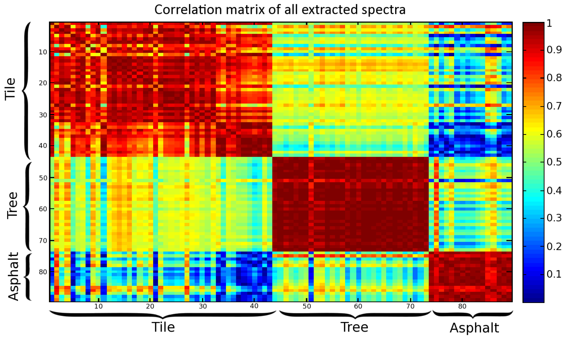
Three main classes of materials are considered: tiles, vegetation and asphalt. For these three classes, a large number of pure spectra can be extracted. It allowed relevant statistical studies.

2.3. Data Analysis

To characterise the intra-class variability, two types of parameters were derived from the extracted spectra: the correlation between spectra and the values of their first two Principal Components. Let $\mathbf{Y}={[{\mathbf{y}}_{\mathbf{1}},\dots ,{\mathbf{y}}_{\mathbf{N}}]}^T$ denote the matrix composed of a set of extracted spectral reflectances, with ${\mathbf{y}}_{\mathbf{n}}\in {\mathbb{R}}^{L\times 1}$ a spectrum, N the number of pixels and L the number of wavelengths. The coefficients of the correlation matrix, $COR{R}_{i,j}$, can be written as follows:

$$COR{R}_{i,j}=\frac{Cov({\mathbf{y}}_{\mathbf{i}},{\mathbf{y}}_{\mathbf{j}})}{{\sigma }_{y_i}{\sigma }_{y_j}}$$

(1)

with $Cov(·,·)$ the covariance between two vectors and ${\sigma }_y$ the standard deviation of the vector $\mathbf{y}$.

Figure 3 contains four correlation matrices. For each of the tree and asphalt correlation matrices (Figure 3c,d), a single area of the sub-image corresponding to a single class was selected. The correlation was computed between all extracted spectra of this area. The tile correlation matrix (Figure 3a) was obtained in the same way, with tiles extracted from the same roof. The extended tile correlation matrix (Figure 3b) was computed between spectra extracted from various areas of the image, including the spectra used in the tile correlation matrix.

The correlation between the spectra extracted from a same roof fluctuates a lot, between $75\%$ and $95\%$, which shows the large variability of the class. The low correlation between some spectra (below $75\%$) is probably due to the non purity of some extracted spectra, resulting from various elements that can be fixed on roofs (gutter, aerial...). These extreme values were removed for the following studies. Analyses of the asphalt correlation matrix are similar to those for the tile correlation matrix. The correlation between neighbouring asphalt spectra can be lower than $80\%$. The variability between spectra is due to different road surfacing. Results for the tree correlation matrices differ from the above results. The correlation between these spectra is higher than $90\%$ (which correspond to a low variability) except for the correlation of several spectra with the 8th spectrum (probably a non pure spectrum). It can be due to the fact that, in this area of Toulouse, most of the trees in streets belong to the same species, namely plane trees. The extended tile correlation matrix, in Figure 3b, was obtained by computing pure spectra of a same material class extracted from various locations of the image. It appears that the correlation between spectra extracted from a same roof is higher, from $75\%$ to $95\%$, than the one between spectra of various roofs, from $65\%$ to $95\%$. The largest observed intra-class variability, in Figure 3 and Figure 4, makes sense as the tiles of Toulouse roofs are not the same (various mineral compositions...). It means that intra-class variability increases when the number of buildings, or independent areas, increases. This result can be extended to other classes of materials like asphalt.

Figure 4 contains the correlation matrix of all extracted spectra, which illustrates both inter and intra-class variabilities. Figure 4 shows the variability at the sub-image scale, since spectra from the same material were extracted from various locations of the sub-image, as for the extended tile correlation matrix in Figure 3. Firstly it appears, as depicted in Figure 3, that the intra-class variability can be low (correlation higher than $80\%$ for the asphalt class). However, it is higher than in Figure 3 for some classes, especially when the class includes spectra extracted from various areas of the images, like tiles. The intra-class variability of a class depends on the observed scene. The tree class frequently has a high intra-class variability. It is not the case here (correlation around $90\%$) since the considered areas contain similar tree species. The second important point is the high correlation between spectra of different classes. This variability is called inter-class variability. This phenomenon has to be considered. Indeed, if some classes have too close spectra, they would be hardly distinguishable especially when those classes have a high intra-class variability. For instance, the correlation between some tile and vegetation spectra is higher than $60\%$, whereas some tile spectra are only $70\%$ correlated. This could lead to confusion between classes. Indeed, if a class is defined by a bundle as in [31], the parameters have to be very carefully chosen to avoid spectra misclassification.

The above correlation coefficients do not show the variability of average level from one spectrum to another, which is highly related to illumination variation. To visualize it, a projection of the extracted spectra onto the first Principal Component Analysis (PCA) axes was performed. Figure 5 illustrates the obtained results. In Figure 5a, spectra of three classes are projected onto the first two principal axes. For the tile class, spectra are extracted from various roof slopes (i.e., various illumination conditions). The tree class is composed of spectra extracted from a same area; however, the illumination of the canopy varies from a tree to another. This class also depicts the effects of illumination on the intra-class variability. The scale factor variability which cannot be seen in Figure 3 and Figure 4 appears clearly in Figure 5. Indeed, the set of spectra ${\mathcal{E}}_m=\{\mathbf{s}\backslash \mathbf{s}=\gamma {\mathbf{r}}_{\mathbf{m}},\gamma \in {\mathbb{R}}^{\ast +}\}$ previously mentioned in Section 2.1 is represented in a PCA projection as a line passing through the origin. In Figure 5b, this scale factor is visible for the sunny tile class. Spectra belonging to each class are more or less located along the same direction. However, they do not exactly form a line. The variations on the axis passing through the origin correspond to the scale factor whereas the variations around this axis are linked to other phenomena. The location of blue and red dots in Figure 5 illustrates this. Indeed, the darkest spectra (red dots) are the closest to the origin and the blue ones are situated further on the axis depending on their illumination. Asphalt projections corroborate this analysis. These spectra are dark ones and are located close to the origin and close to the spectra of dark trees and tiles.

Taking these observations into account, it appears that the intra-class variability has to be considered to perform an accurate unmixing. These investigations also show that the modelling of the intra-class variability by a scale factor is not sufficient. Thus, in the following sections, a new mixing model dealing with intra-class variability is developed as well as unmixing methods adapted to this model.

3. Unmixing Problem Statement

In the standard linear mixing model (LMM), each sensed spectrum ${\mathbf{x}}_{\mathbf{p}}\in {\mathbb{R}}^{L\times 1}$ can be written as follows:

$${\mathbf{x}}_{\mathbf{p}}=\sum _{m=1}^M{c}_{pm}{\mathbf{r}}_{\mathbf{m}}\forall p\in \{1,\dots ,P\},$$

(2)

where p is the pixel index, P the number of pixels, m the index of one of the M endmembers, ${\mathbf{r}}_{\mathbf{m}}\in {\mathbb{R}}^{L\times 1}$ is the mth source spectrum and $c_{pm}$ is the associated mixing coefficient. The above model does not take into account intra-class variability. We introduce a new extended mixing model, which reads:

$${\mathbf{x}}_{\mathbf{p}}=\sum _{m=1}^M{c}_{pm}{\mathbf{r}}_{\mathbf{m}}(p)\forall p\in \{1,\dots ,P\},$$

(3)

where ${\mathbf{r}}_{\mathbf{m}}(p)$ is the spectrum associated with the mth source and pixel p. Extracting these sources from such observations is an ill-posed problem. In Equations (2) and (3), we add the classical sum-to-one constraint (besides the nonnegativity constraint). This condition leads to:

$$\sum _{m=1}^M{c}_{pm}=1\forall p\in \{1,\dots ,P\}.$$

(4)

Let $\mathbf{X}={[{\mathbf{x}}_{\mathbf{1}},\dots ,{\mathbf{x}}_{\mathbf{P}}]}^T$ denote the sensed spectrum matrix, $\mathbf{R}={[{\mathbf{r}}_{\mathbf{1}},\dots ,{\mathbf{r}}_{\mathbf{M}}]}^T$ the endmember matrix if there is no intra-class variability (same sources for all pixels) and $\mathbf{C}={[{\mathbf{c}}_{\mathbf{1}},\dots ,{\mathbf{c}}_{\mathbf{P}}]}^T$ the mixing coefficient matrix. For all pixels p, ${\mathbf{c}}_{\mathbf{p}}={[c_{p1},\dots ,c_{pM}]}^T$ is an M-element vector containing the set of mixing coefficients associated with the pth observed spectrum. The number of sources, M, is assumed to be known in the rest of the paper. The LMM can be written as follows:

$$\mathbf{X}=\mathbf{CR}.$$

(5)

To obtain a similar expression from model (3), we introduce $\mathbf{R}(p)={[{\mathbf{r}}_{\mathbf{1}}(p),\dots ,{\mathbf{r}}_{\mathbf{M}}(p)]}^T$, the set of M sources associated with the observed spectrum ${\mathbf{x}}_p$, $\tilde{\mathbf{R}}=\left[\begin{array}{c}\mathbf{R}(1)\\ \dots \\ \mathbf{R}(P)\end{array}\right]\in {\mathbb{R}}^{PM\times L}$, the matrix containing all the sources and $\tilde{\mathbf{C}}\in {\mathbb{R}}^{P\times PM}$ a block-diagonal matrix denoting the new mixing coefficient matrix:

$$\tilde{\mathbf{C}}=\left[\begin{array}{cccc}{\mathbf{c}}_{\mathbf{1}}^T& 0\dots 0& \dots & 0\dots 0\\ 0\dots 0& {\mathbf{c}}_{\mathbf{2}}^T& \dots & 0\dots 0\\ & & \ddots & \\ 0\dots 0& 0\dots 0& \dots & {\mathbf{c}}_{\mathbf{P}}^T\end{array}\right].$$

(6)

Thus, Equation (3) yields the matrix expression:

$$\mathbf{X}=\tilde{\mathbf{C}}\tilde{\mathbf{R}}.$$

(7)

We aim at retrieving matrices $\tilde{\mathbf{C}}$ and $\tilde{\mathbf{R}}$ under the nonnegativity and sum-to-one constraints.

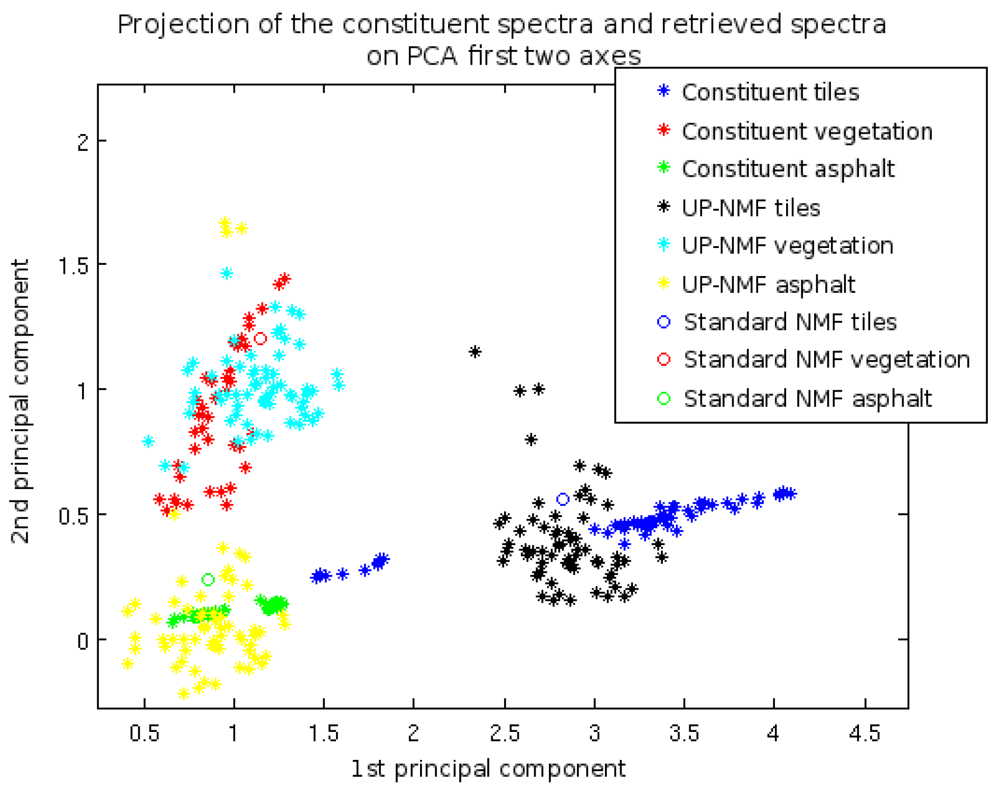
4. Unconstrained Pixel-By-Pixel Nonnegative Matrix Factorisation (UP-NMF)

Nonnegative Matrix Factorisation (NMF) has been adapted to solve remote sensing unmixing problems corresponding to the LMM [35,36]. NMF then aims at decomposing the observation matrix $\mathbf{X}$ as a product of two nonnegative matrices, namely the coefficient matrix, $\mathbf{C}$ and the reflectance matrix, $\mathbf{R}$. The necessary assumption of this method is the nonnegativity of the two searched matrices. The sum-to-one constraint can be added to NMF. To perform NMF, a cost function, hereafter called $J_{nmf}$, is minimised. However, the obtained minima may be local ones. This problem can be overcome with a good initialisation. This will be discussed in a later part (Section 6).

Now considering the extended mixing model (7), we introduce two evolutions of NMF for estimating $\tilde{\mathbf{C}}$ and $\tilde{\mathbf{R}}$. These two methods are respectively defined in this section and in Section 5.

4.1. Cost Function

Standard NMF aims at minimising the reconstruction error (RE) to extract a set of endmembers from a set of observed spectra. The standard cost function can be written as:

$$J_{nmf}=\frac{1}{2}{∥\begin{array}{c}\mathbf{X}-\mathbf{C}\mathbf{R}\end{array}∥}_F^2,$$

(8)

where ${∥\begin{array}{c}.\end{array}∥}_F$ is the Frobenius norm. In Equation (8), $\mathbf{C}$ and $\mathbf{R}$ represent the adaptive variables which respectively aim at estimating the actual coefficients and source spectra involved in the mixing model (5). By using $\tilde{\mathbf{C}}$ and $\tilde{\mathbf{R}}$ instead of $\mathbf{C}$ and $\mathbf{R},$ we extract one set of sources from each sensed spectrum. To this end, the unconstrained pixel-by-pixel NMF (UP-NMF) method is an evolution of standard NMF which minimises the new cost function defined as:

$$J_{upnmf}=\frac{1}{2}{∥\begin{array}{c}\mathbf{X}-\tilde{\mathbf{C}}\tilde{\mathbf{R}}\end{array}∥}_F^2.$$

(9)

As in (8), $\tilde{\mathbf{C}}$ and $\tilde{\mathbf{R}}$ are adaptive variables which aim at estimating the actual coefficients and source spectra in the mixing model (7).

4.2. Gradient Calculation

To minimise $J_{upnmf}$, we developed an extended version of Lin’s standard NMF algorithm [37]. Lin’s method is based on projected gradient. Thus, we have to determine the derivatives of $J_{upnmf}$ with respect to $\tilde{\mathbf{R}}$ and $\tilde{\mathbf{C}}$. These derivatives are easily calculated with the matrix formulas in [38]. To this end, we first rewrite the considered cost function as:

$$J_{upnmf}=\frac{1}{2}Tr((\mathbf{X}-\tilde{\mathbf{C}}\tilde{\mathbf{R}}){(\mathbf{X}-\tilde{\mathbf{C}}\tilde{\mathbf{R}})}^T)$$

(10)

and we then derive:

$$\begin{array}{cc}\hfill \frac{\partial J_{upnmf}}{\partial \tilde{\mathbf{R}}}& =-{\tilde{\mathbf{C}}}^T(\mathbf{X}-\tilde{\mathbf{C}}\tilde{\mathbf{R}}),\hfill \end{array}$$

(11)

$$\begin{array}{cc}\hfill \frac{\partial J_{upnmf}}{\partial \tilde{\mathbf{C}}}& =-(\mathbf{X}-\tilde{\mathbf{C}}\tilde{\mathbf{R}}){\tilde{\mathbf{R}}}^T.\hfill \end{array}$$

(12)

4.3. Update Algorithm

The above calculations allow us to formulate the UP-NMF update algorithm. We choose to use a gradient descent algorithm. The update rules for $\tilde{\mathbf{R}}$ and $\tilde{\mathbf{C}}$ may therefore be expressed as follows:

$$\begin{array}{cc}\hfill {\tilde{\mathbf{R}}}^{(i+1)}& ⟵{\tilde{\mathbf{R}}}^{(i)}-{\alpha }_{\tilde{\mathbf{R}}}\frac{\partial J_{upnmf}^{(i)}}{\partial \tilde{\mathbf{R}}},\hfill \end{array}$$

(13)

$$\begin{array}{cc}\hfill {\tilde{\mathbf{C}}}^{(i+1)}& ⟵{\tilde{\mathbf{C}}}^{(i)}-{\alpha }_{\tilde{\mathbf{C}}}\frac{\partial J_{upnmf}^{(i)}}{\partial \tilde{\mathbf{C}}},\hfill \end{array}$$

(14)

followed by projection onto ${\mathbb{R}}^{+\ast }$ and sum-to-one normalisation. ${\alpha }_{\tilde{\mathbf{R}}}$ and ${\alpha }_{\tilde{\mathbf{C}}}$ are positive adaptation steps.

Using (11) and (12), we obtain the update rules for our UP-NMF method. However, only all ${\mathbf{c}}_{\mathbf{p}}^T$ in (6) should thus be updated, whereas the other terms of $\tilde{\mathbf{C}}$ are kept to zero. The pseudo-code of the complete UP-NMF update thus obtained is provided in Appendix A.

Due to the high underdeterminacy of this optimisation problem, the behavior of UP-NMF is not accurate enough. Estimated spectra ${\mathbf{r}}_{\mathbf{m}}(p)$ from a same class m may evolve so differently that they tend to define several classes of materials. This observation is all the more important that the inter-class variability is small, as it was explained in Section 2.3. To limit this spreading of estimated spectra from a same class, constraints are required in the cost function. Such a constraint is proposed hereafter, in Section 5. It is based on the observations made in Section 2.3 and aims at penalising the spreading of estimated sources from the same class.

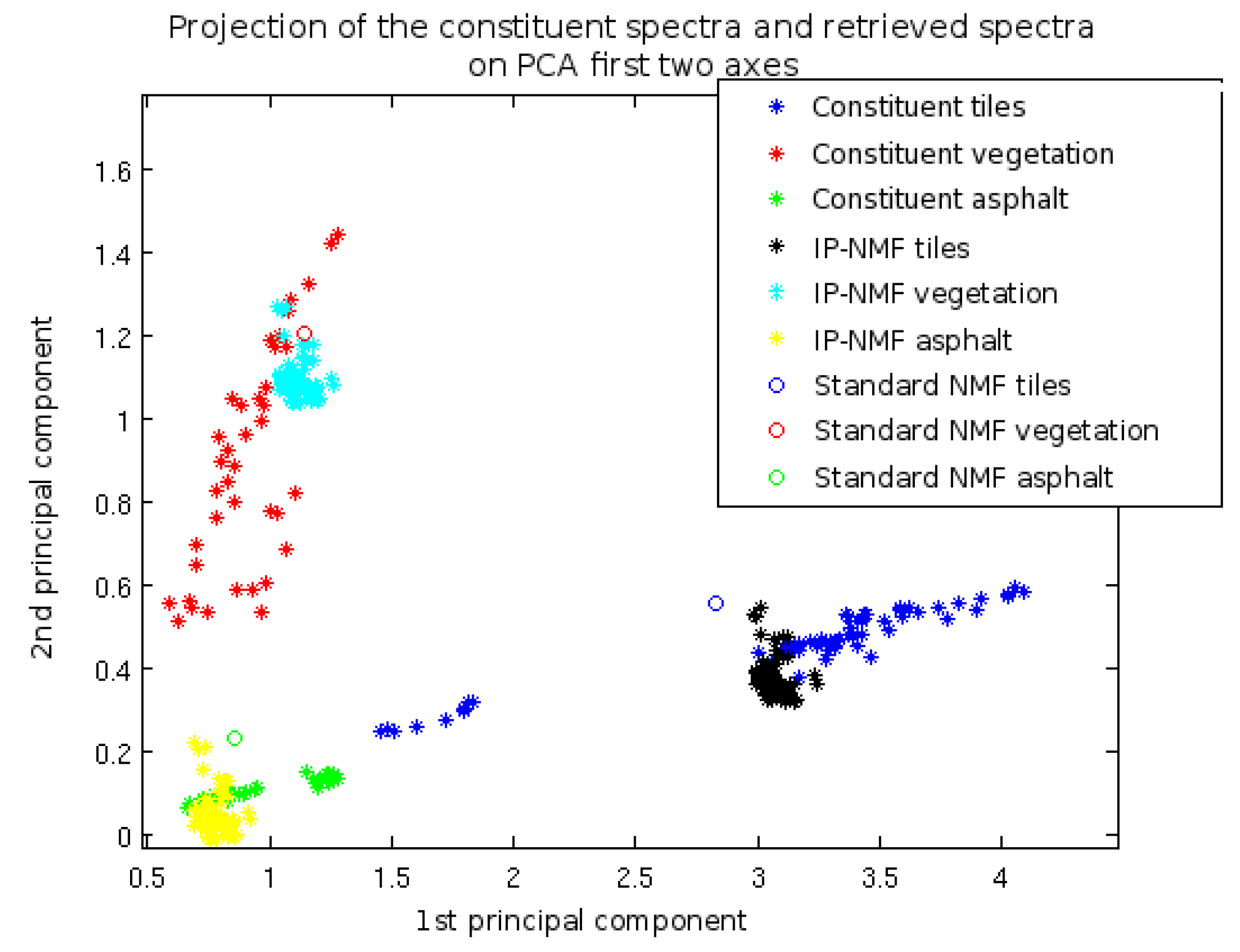
5. Inertia-Constrained Pixel-By-Pixel Nonnegative Matrix Factorisation (IP-NMF)

5.1. Cost Function

Our second method is based on limiting class inertia to reduce the risk for an estimated pure spectrum to go out of its own class. This limitation is introduced in the optimisation problem by adding a penalty term in the cost function. The function to be minimised thus becomes:

$$J_{ipnmf}=\frac{1}{2}{∥\begin{array}{c}\mathbf{X}-\tilde{\mathbf{C}}\tilde{\mathbf{R}}\end{array}∥}_F^2+\mu \sum _{m=1}^{M}Tr(Cov({\tilde{\mathbf{R}}}_{{\mathcal{C}}_{\mathbf{m}}})),$$

(15)

where ${\tilde{\mathbf{R}}}_{{\mathcal{C}}_{\mathbf{m}}}\in {\mathbb{R}}^{P\times L}$ is the matrix containing estimates of all the endmembers of the mth class (i.e., spectra of the mth material), $Tr(Cov({\tilde{\mathbf{R}}}_{{\mathcal{C}}_{\mathbf{m}}}))$ is the inertia of the mth class and $\mu$ is the constraint parameter. We compute ${\sum }_{m=1}^{M}Tr(Cov({\tilde{\mathbf{R}}}_{{\mathcal{C}}_{\mathbf{m}}}))$ rather than $Tr(Cov(\tilde{\mathbf{R}}))$ because the latter expression tends to aggregate all classes. The trace of the covariance matrix measures the spreading of the spectra constituting the matrix, whatever the gravity center is. By using this penalty term, estimated spectra moving too far away from others during their adaptation by our unmixing method penalise the whole class. The proposed penalty term therefore enforces the homogeneity of estimated spectra from the same class. Thus, it can be expected that the spectra estimated by our method, which were derived from the same “seed”, still define the same class.

5.2. Gradient Calculation

To minimise $J_{ipnmf}$, we develop an extended version of Lin’s standard NMF algorithm [37], as for UP-NMF. Thus, here again, we have to determine the derivatives of the cost function with respect to $\tilde{\mathbf{R}}$ and $\tilde{\mathbf{C}}$. The corresponding calculations are provided in Appendix B.

5.3. Update Algorithm

The calculations provided above allow us to formulate the associated update algorithm. The general gradient descent formulation was already given in (13) and (14). Using it, we here obtain the update rules for our IP-NMF method. As for UP-NMF, only the ${\mathbf{c}}_{\mathbf{p}}^T$ in (6) should thus be updated, whereas the other terms of $\tilde{\mathbf{C}}$ are kept to zero. Thus, the complete IP-NMF update can be written as follows:

Algorithm 1: 1 Update of matrix $\tilde{\mathbf{R}}$

As all iterative algorithms, IP-NMF as UP-NMF have to be initialised. The choices we made are described in Section 6.1.

6. Test Results for Semi-Synthetic Data Set

6.1. Test Description

Tests of the UP-NMF and IP-NMF methods are firstly performed with semi-synthetic data. The sources are real spectra extracted from the hyperspectral sub-image described in Section 2.2. They are shown in Figure 1. They describe realistic source variations. Mixing coefficients are randomly chosen while respecting the sum-to-one constraint. The mixing model is defined by Equation (3).

Tests are performed by varying the initial matrices ${\tilde{\mathbf{R}}}^{(0)}$ and ${\tilde{\mathbf{C}}}^{(0)}$ and the constraint parameter $\mu$. Three matrices ${\tilde{\mathbf{R}}}^{(0)}$ are tested: (i) M mixed signals randomly selected from the observations; (ii) the M purest signals extracted with a classical remote sensing blind source separation method (N-FINDR [39]); (iii) for each class m, the average of all P source signals in this class. Two methods are successively used for initialising the mixing coefficient matrix ${\tilde{\mathbf{C}}}^{(0)}$: (a) giving the same constant value, $\frac{1}{M}$, to all coefficients; (b) extracting coefficients associated with initial spectra, by means of a Fully Constrained Least Square (FCLS) regression [40,41,42]. The constraint parameter $\mu$ varies from 0 to 100, to assess the impact of $\mu$ on the algorithm performance.

Among the above listed initialisations, only the results for one couple are discussed in the first part of Section 6.3, namely ${\tilde{\mathbf{R}}}^{(0)}$ and ${\tilde{\mathbf{C}}}^{(0)}$ respectively initialised by (ii) and (a). Indeed, (i) is a more uncertain initialisation than (ii), whereas (iii) is the best expected initialisation of ${\tilde{\mathbf{R}}}^{(0)}$, but it requires knowledge about the data, which is not available for real data sets. Method (a) was chosen to initialise ${\tilde{\mathbf{C}}}^{(0)}$ to reduce the risk of being in a local minimum (this conclusion results from a study of UP-NMF and IP-NMF initialised with (b)).

6.2. Evaluation Criteria

Chosen criteria assess the benefits of our unmixing methods. A major feature to be evaluated is the fit between estimated pure material reflectance spectra and pure spectra really present in each pixel. To this end, we computed, in each pixel p, the spectral angles between these two sets of M spectra [27]. The resulting criterion is defined as:

$$SAM(p)=\frac{1}{M}\sum _{m=1}^M({cos}^{-1}\left(\frac{\langle {\mathbf{r}}_{\mathbf{m}}(p),{\widehat{\mathbf{r}}}_{\mathbf{m}}(p)\rangle }{\parallel {\mathbf{r}}_{\mathbf{m}}{(p)\parallel }_2·{\parallel {\widehat{\mathbf{r}}}_{\mathbf{m}}(p)\parallel }_2}\right)),$$

(16)

where $\langle ·,·\rangle$ stands for the scalar product, ${\mathbf{r}}_{\mathbf{m}}(p)$ is the spectrum of the mth source really present in the pth pixel and ${\widehat{\mathbf{r}}}_{\mathbf{m}}(p)$ is the estimated one (to determine which estimated spectrum corresponds to which actual spectrum ${\mathbf{r}}_{\mathbf{m}}(p)$, one may compute, for each considered estimated spectrum, the SAMs of that considered estimated spectrum successively with each of the actual spectra ${\mathbf{r}}_{\mathbf{m}}(p)$ and keep the spectrum ${\mathbf{r}}_{\mathbf{m}}(p)$ which yields the lowest SAM, since it corresponds to the best fit). The spectral angle error $SAM(p)$ is then averaged over all pixels to obtain the mean spectral error, denoted as $SAM$. If the shapes of two spectra ${\mathbf{r}}_{\mathbf{m}}(p)$ and ${\widehat{\mathbf{r}}}_{\mathbf{m}}(p)$ are very similar, the corresponding value $SAM(p)$ is close to 0.

Two other criteria were also computed. The first one is the reconstruction error, $RE$, which evaluates the performance of our method in terms of the global reconstruction of the image. In the same way as for the spectral error, the reconstruction error is computed at pixel level as

$$RE(p)=\frac{1}{L}·{\parallel {\mathbf{x}}_{\mathbf{p}}-{\widehat{\mathbf{c}}}_{\mathbf{p}}^T\widehat{\mathbf{R}}(p)\parallel }_F$$

(17)

and then averaged over all the image, thus yielding the $RE$ parameter. The second considered criterion is the mean square error computed over all mixing coefficients and denoted as $CE$, for “coefficient error”. As for $RE$ and $SAM$, it can be computed at pixel level as

$$CE(p)=\frac{1}{M}·{\parallel {\mathbf{c}}_{\mathbf{p}}-{\widehat{\mathbf{c}}}_{\mathbf{p}}\parallel }_F$$

(18)

and then averaged over all the image, thus yielding the $CE$ parameter. Computing these errors is possible for semi-synthetic data for which the sources and mixing parameters are known.

6.3. Results

Figure 6 illustrates the sources used in the mixing (blue, red and green stars) compared with UP-NMF results (black, cyan and yellow stars) and standard NMF results (blue, red and green circles). Figure 7 and Figure 8 illustrate the same comparisons for IP-NMF with $\mu$ equal to 30 and 100, respectively. For these three figures, ${\tilde{\mathbf{R}}}^{(0)}$ is built with N-FINDR results and ${\tilde{\mathbf{C}}}^{(0)}$ with constant coefficients $\frac{1}{M}$.

For each class, the scatter plots of the actual and extracted spectra should be superimposed up to scale factors. Indeed, scale factors can be contained in the estimated spectra and respectively the inverse in the associated estimated abundances:

$${\mathbf{x}}_{\mathbf{p}}=\sum _{m=1}^M\frac{1}{k_m(p)}{c}_{pm}\times k_m(p){\mathbf{r}}_{\mathbf{m}}(p)\forall p\in \{1,\dots ,P\}.$$

(19)

Hence, dots can move onto the axes passing through the origin. Thus, the dot position onto its class main axis depends on its estimated scale factor.

As mentioned in Section 4, the main risk is spectra spreading. The magnitude of the spreading of a class can be measured by the variance of the projection of this class plot onto the line which contains the center of gravity of that class plot and which is orthogonal to the line which contains that center of gravity and the origin. This spreading clearly appears in Figure 6, where the above-defined variances of the retrieved spectra are high as compared with the variances of the spectra actually used to create the processed mixed spectra. This reinforces our idea to limit the class inertia. Results in

Table 1. Global comparison of unmixing methods.

	N-FINDR + FCLS	Standard NMF	UP-NMF	IP-NMF ($\mathbf{\mu }=30$)	IP-NMF ($\mathbf{\mu }=100$)
$RE$	$17.5$	$0.6$	<0.1	$2.9$	$4.4$
$SAM$ (deg)	$7.7$	$7.7$	$9.4$	$5.5$	$6.1$
$CE$ (%)	$4.0$	$4.7$	$3.8$	$3.8$	$3.8$
Time (s)	$0.03$	$0.02$	$5.87$	$5.90$	$6.48$

confirm this observation. In this table, results of UP-NMF and IP-NMF (with $\mu$ fixed to 30 and 100) were compared to standard NMF and a classical unmixing method (N-FINDR [43] + FCLS [40]). The average $SAM$ of the UP-NMF method is the highest, whereas its $RE$ is the lowest. The lowest value of $RE$ is due to the fact that the cost function of UP-NMF (or IP-NMF with $\mu =0$) is the $RE$, with the largest degree of freedom to minimize it. However, this freedom is to the detriment of physical significance of the retrieved spectra, as even the data noise can be fitted to minimize $RE$, leading to an “overfitting” of the data. This is the reason why $SAM$ is higher. This is illustrated in Figure 6. For instance, endmembers of the tiles retrieved by UP-NMF spread far from the solution. Similar observations can be made for asphalt and vegetation. This result is also illustrated in Figure 9 for low values of $\mu$. As $\mu$ increases, the weight of $RE$ in the cost function decreases, which leads to an increase in the final $RE$, but for moderate values of $\mu$, as the constraint on intra-class variability grows up, it limits the spectral variability of the endmembers and thus avoids the risks of retrieving irrelevant spectra. The tightening of the pixel clouds close to the true spectra is visible in Figure 7. For intermediate values of $\mu$, that is in the domain ranging from 30 to 80, the performance, in terms of spectral angle, is good and quite stable (see Figure 9 and Table 1), but, logically, $RE$ increases. For high values of $\mu$ (higher than 80), both $CE$ and $SAM$ increase because the cost function is driven by the inertia constraint, while the reconstruction of data with appropriate endmembers plays a too minor role. Thus, the final endmembers will stay close to the initial spectra, with a decrease of cloud spreading (see Figure 8). The $CE$ criterion is less discriminant to evaluate the tested methods, but the worst score is obtained for standard $MNF$. Among the three criteria, the $SAM$ and the $CE$ are the most relevant for classification and identification methods based on spectral signature, and for mapping purposes. As a consequence, the method giving the best performance is IP-NMF with $\mu$ around 30 ($SAM=5.5^{\circ }$ and $CE=3.8\%$). The computational times of UP-NMF and IP-NMF are significantly higher than those of these two standard methods. However, the structure of the proposed algorithm makes it quite easily parallelisable. The time variations between the three cases are caused by the fluctuations of the number of iterations.

The second point consists of analysing the impact of initialisation. We applied IP-NMF with the initialisation scenarios described in Section 6.1. It appears that a poor initialisation (scenario (i)) leads to poor results for both the standard NMF, UP-NMF and IP-NMF. However, compared with standard NMF, IP-NMF improves the average spectral angle error in every initialisation case. We also noted that, if both the spectra and the abundance coefficients are initialised too close to a local minimum (scenario (iii) and (b)), the results of our methods are close to this initialisation.

7. Test Results for Real Images

7.1. Data Set

In this study, we focus on an image of the city center. A sub-image was extracted from the larger image shown in Figure 2 and described in Section 2.2. It contains an avenue, vegetation (trees and grass), tile roofs and shadows of these materials. Figure 10 shows this sub-image.

7.2. Test Description

Several methods were tested on this data set:

• Two classical geometric methods: VCA [30] and N-FINDR [39] extract endmembers (one per class of materials). The abundances are then retrieved by a usual Fully Constrained Least Square (FCLS) algorithm [41,42].
• A standard NMF method [37] is applied to retrieve at the same time both the source spectra (one per class) and their associated abundance coefficients.
• IP-NMF is applied to obtain one set of endmembers per pixel and the associated coefficients.

IP-NMF requires the number of classes, M. To find it, a well-known method, HySime, developed by Bioucas-Dias et al. in [44], was tested to identify the number of endmembers in the considered hyperspectral image. The results of HySime lead to 46 endmembers. This over-determination of the endmember extraction is due to the intra-class variability. Indeed, HySime does not take this phenomenon into account (at least, not enough). The aim of IP-NMF is to work with a limited and realistic number of classes. Thus, HySime cannot be used here to initialise M. It will be manually initialised. In these tests, IP-NMF is applied with various parameter initialisations. Figure 11 shows that the observed scene mainly consists of three classes: asphalt (red and yellow classes in Figure 11), vegetation (cyan, magenta and dark green in Figure 11) and tiles (green class in Figure 11). Some particular elements could be problematic (the car (blue class in Figure 11), the track (purple class in Figure 11), and the roof elements (mixed in the tile pixels)...). Thus, the number of endmembers, M, is successively fixed to 3, 5 and 7. In order to create a fully automated algorithm, the initialisation of spectra is firstly obtained with the VCA method. As a comparison, a second initialisation with manually selected spectra is also performed. Thanks to this manual selection of pure spectra, we obtain one of the best possible initialisations. The coefficients are initialised with the constant value $\frac{1}{M}$ since this initialisation was the one yielding the best results for the semi-synthetic data tests (cf. Section 6.3). Considering Figure 9, the $SAM$ only moderately varies when $\mu$ ranges between 20 and 80. Thus, a constant $\mu$ was fixed for all the following tests, equal to 30, as for the semi-synthetic data tests.

Evaluation criteria cannot be the same here as those used for the semi-synthetic data tests. Indeed, due to the lack of ground truth, we cannot compute the $SAM$ and $CE$ errors. Therefore, only the Reconstruction error, $RE$, and a usual analysis of the results in various ways (PCA projection, abundance maps...) can be considered. It was decided not to exploit the $RE$ because of the reasons developed in Section 6.3.

7.3. Results

IP-NMF was applied with the two initialisations described in the previous subsection. Results are provided in Figure 12, Figure 13 and Figure 14. Each of these figures shows the abundance maps of VCA + FCLS unmixing (1st line), NMF (2nd line), IP-NMF initialised with VCA (3rd line) and IP-NMF manually initialised (4th line) applied with M equal to 3, 5 and 7 respectively in Figure 12, Figure 13 and Figure 14. The results obtained with N-FINDR are not shown because they are very close to those obtained with VCA.

7.3.1. Results of Classical Unmixing Methods (One Set of Endmembers per Image)

As described previously, two methods were applied to the image, namely VCA + FCLS and a standard NMF. Abundance maps are shown in the 1st and 2nd lines of Figure 12, Figure 13 and Figure 14. It appears that VCA + FCLS and NMF maps are relatively similar. This is due to the initialisation, since NMF was initialised with spectra obtained with VCA. Several observations are made hereafter from these maps.

Firstly, the asphalt class (road) is never accurately extracted: in the three figures, the extracted asphalt class is a mixture of the shadow endmember and another one. For instance, in Figure 12, it is a mixture of the shadow endmember and the tile endmember. Then, increasing the number of endmembers reduces the unmixing quality because these unmixing methods then sometimes focus on specific spectra (vertices of the simplex), instead of extracting all major classes. It is the case in Figure 13 and Figure 14 where a car spectrum is extracted (2nd column and 1st column respectively in Figure 13 and Figure 14). Conversely, due to intra-class variability, several extracted endmembers can in fact belong to the same class: this e.g., occurs for the tiles in Figure 14 (5th and 6th columns).

For this image, it seems that Figure 12 yields the best results. Indeed, it provides all classes except the road. However, the vegetation thus extracted (3rd column) is not uniform.

7.3.2. Results of the IP-NMF Method Initialised with VCA

To analyse the results of the “automated” IP-NMF method, the 3rd line of Figure 12, Figure 13 and Figure 14 is studied. First of all, it has to be noted that, even if abundance maps are presented in the same way for VCA, NMF and IP-NMF, they represent different phenomena. Indeed, for VCA and NMF, each map is associated with a single endmember, whereas for IP-NMF a map is associated with a class. This means that each abundance of IP-NMF abundance maps is associated with a spectrum different from its neighbours. The understanding of the results is highly linked to this preliminary remark.

Our first observation concerning Figure 12 is the homogeneity of areas: contrary to the VCA and NMF results, there is no cyan background in the maps, which would correspond to a material weakly present in a large number of pixels. This is the result of the introduction of degrees of freedom for modelling intra-class variability in our adaptive variables corresponding to $\tilde{\mathbf{C}}$ and $\tilde{\mathbf{R}}$. The three classes obtained with IP-NMF are: shadowed asphalt (1st column), sunny asphalt + tiles (2nd column), vegetation (3rd column). The 2nd class contains spectra of asphalt and tiles. This result is the consequence of two things: the low inter-class variability (cf. Section 2.3) and the initialisation. Indeed, due to the low inter-class variability, constituent spectra are spectrally close even if they do not belong to the same class. Thus, it is possible that, in the same class, estimated spectra evolve in different ways and form two clusters, i.e., two sub-classes inside one class. This is what happens in this test. This is possible since the distance between the two centers of gravity of the sub-classes is similar to the intra-class variability of some classes. Initialisation is also accountable for this phenomenon, since all the spectra of a class evolved from a same “seed spectrum”. Thus, if the initialisation spectrum (or “seed spectrum”) is close to the two classes, this phenomenon more easily appears.

Since this phenomenon is due to the combination of two classes which are spectrally too close, what happens when the number of classes is increased? This is depicted in Figure 13 and Figure 14. It can be observed that the results are not as expected. Indeed, new classes appear—for instance, the car (Figure 13, 2nd column and Figure 14, 1st column), but the quality of the unmixing decreases. For instance, the road is now considered as a mixture of two spectra. This decrease of the quality is due to the initialisation, as will be shown in Section 7.3.3. Indeed, the VCA spectra are used to initialise IP-NMF and the poor quality of spectra extracted by VCA influences the results of IP-NMF, in which spectra cannot move enough to compensate for the initialisation error. However, IP-NMF gives better results than VCA or NMF. Indeed, some classes are detected only by IP-NMF. In addition, sometimes spectra in a pixel are misclassified by IP-NMF (i.e., they do not belong to the same physical class as other spectra of this class), but anyway they accurately fit the actual pure spectra present in this pixel.

7.3.3. Results of the IP-NMF Method with Manual Initialisation

The 4th line of Figure 12, Figure 13 and Figure 14 shows the impact of the initialisation on IP-NMF results. IP-NMF was initialised respectively by 3, 5 and 7 spectra manually selected in the image. This allows one to choose the initial classes and ensures that initialisation spectra are pure ones. In Figure 12, selected spectra were a tile spectrum, an asphalt spectrum and a tree spectrum. Abundance maps show that the tiles are very well extracted (column 1 of Figure 12 compared to the sub-image of Figure 10). Asphalt is quite well extracted (column 2 of Figure 12), but the road is not as homogeneous as the road extracted by automated IP-NMF (row 3, column 2 of Figure 12). The 3rd extracted class (column 3 of Figure 12) contains vegetation and shadowed asphalt. As in the previous case (automated IP-NMF), abundance maps show a combination of two subclasses in a class. With this manual initialisation, an improvement of the result is expected when the number of classes is increased because the quality of automated IP-NMF results falls due to the poor initialisation given by VCA. In Figure 14, seven classes of spectra were extracted: tile, asphalt, shadowed asphalt, tree, grass, shadowed tree, and path (resp. columns 1 to 7 of Figure 14). Compared to the automated IP-NMF results, the extraction of some classes is better performed here. Tiles are well retrieved despite their high variability, as the asphalt. However, the vegetation extraction is better with the automated IP-NMF: the grass (5th column) and tree (4th column) classes compete, which leads to poor tree extraction here. In addition, the shadowed trees and shadowed tiles are extracted in the same class (7th column) due to their spectral proximity.

Thus, it seems that a manual initialisation of the spectra with spectra belonging to expected classes improves the extraction of classes with high intra-class variability (tiles). However, when intra-class variability is smaller, this initialisation can lead to lower performance than the automated one. For instance, shadowed trees have a small inertia compared with the tiles, so the shadowed tree class can grow and other shadowed spectra are absorbed. However, these spectra are still spectrally different, even if they belong to the same class.

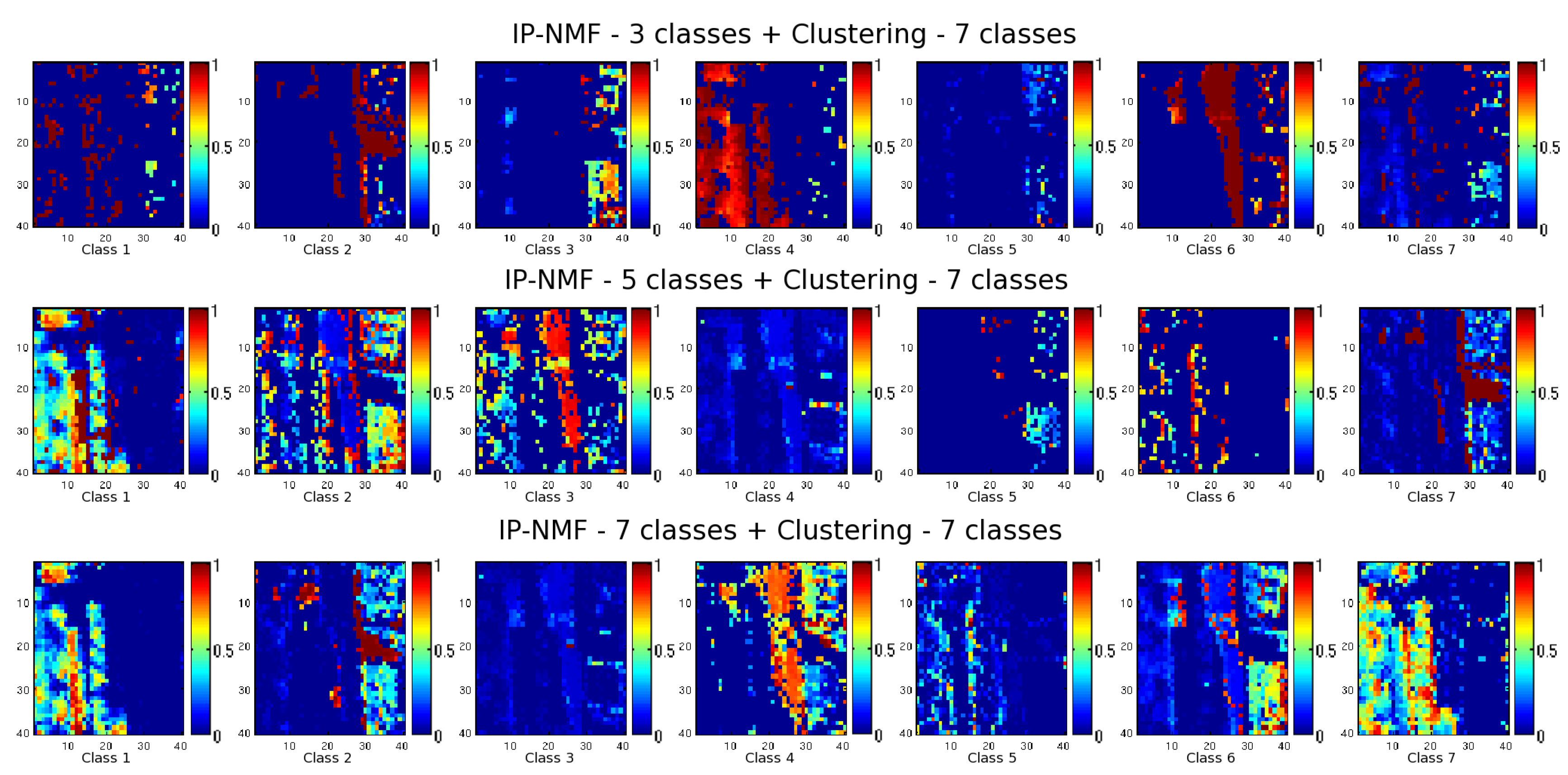
7.3.4. Result of Automated IP-NMF with a Post-Processing

Even with a good initialisation, some problems persist. We propose to solve them by keeping the above automated IP-NMF method, followed by a post-processing stage. We exploit the fact that each pixel is described by a unique set of endmembers. After applying IP-NMF, we gathered all these spectra and then clustered them with the k-means method [45] using spectral angle as the similarity measure. For each pixel, we thus restructure the estimated spectra, and therefore the associated abundances, with respect to the considered set of classes derived by the k-means method. For each of these classes, we then derive the associated abundance map. These abundance maps are shown in Figure 15.

This post processing appears to be all the more efficient as the number of endmembers searched by IP-NMF is small. Indeed, modifications of the maps between Figure 14, 3rd line and Figure 15, 3rd line (with classes extracted in arbitrary orders) are small compared to the differences between Figure 12, 3rd line and Figure 15, 1st line. This post-processing allows us splitting the classes composed of two subclasses. For instance, in the $M=3$ case, tile class and asphalt class are well separated. This post processing therefore allows one to further exploit the large amount of information extracted by IP-NMF, by improving the classification of the extracted pure spectra. Other post-processing methods can be imagined for other applications which would exploit the high number of spectra extracted with IP-NMF.

8. Conclusions

In this paper, intra-class variability was first studied in order to characterise its magnitude. This analysis led us to develop a new mixing model taking this phenomenon into account. Two blind unmixing methods were then introduced to deal with intra-class variability. Tests on semi-synthetic data showed that UP-NMF has lower performance than IP-NMF. IP-NMF performance was also assessed with a real image. To process hyperspectral images, IP-NMF has the advantage of being automated; only the number of classes needs to be fixed. When initialisation of this method is provided by a usual unmixing method, IP-NMF always yields better performance than the latter method in our tests. Indeed, IP-NMF brings its flexibility to find endmembers around the single spectrum per class used to initialise it. The sensitivity of IP-NMF to the initial number of classes is lower than that of the considered classical unmixing methods. In addition, IP-NMF is able to find classes which were not detected by the above classical methods. This makes IP-NMF more robust to processing real images. In addition, to increase the accuracy of the results and to exploit the large number of endmembers provided by IP-NMF, a post-processing stage can be added. Moreover, if users of this method agree to act on the algorithm, a manual initialisation could also be used instead of the above automated initialisation. This kind of initialisation allows the users to choose their classes of interest.

Our method is an extension of NMF. We chose to use a gradient descent to obtain our estimated spectra and abundances. Variants of this method may be developed by using other optimisation algorithms. The cost function optimised in this version penalises the spread of classes. Other versions could be imagined which would penalise the cost function with other terms (distance to the initial spectrum, introduction of spatial constraints...). We plan to develop such versions and to compare them with the UP-NMF and IP-NMF methods.

References

1. Keshava, N.; Mustard, J. Spectral unmixing. IEEE Signal Process. Mag. 2002, 19, 44–57. [Google Scholar] [CrossRef]
2. Singer, R.B.; McCord, T.B. Mars—Large scale mixing of bright and dark surface materials and implications for analysis of spectral reflectance. In Proceedings of the Lunar and Planetary Science Conference, Houston, TX, USA, 19–23 March 1979; Volume 10, pp. 1835–1848. [Google Scholar]
3. Meganem, I.; Deliot, P.; Briottet, X.; Deville, Y.; Hosseini, S. Linear Quadratic Mixing Model for Reflectances in Urban Environments. IEEE Trans. Geosci. Remote Sens. 2014, 52, 544–558. [Google Scholar] [CrossRef]
4. Mustard, J.F.; Pieters, C.M. Quantitative abundance estimates from bidirectional reflectance measurements. J. Geophys. Res. 1987, 92, E617–E626. [Google Scholar] [CrossRef] [Green Version]
5. Bioucas-Dias, J.; Plaza, A.; Dobigeon, N.; Parente, M.; Du, Q.; Gader, P.; Chanussot, J. Hyperspectral Unmixing Overview: Geometrical, Statistical, and Sparse Regression-Based Approaches. IEEE J. Sel. Top. Appl. Earth Obs. Remote Sens. 2012, 5, 354–379. [Google Scholar] [CrossRef] [Green Version]
6. Heylen, R.; Parente, M.; Gader, P. A Review of Nonlinear Hyperspectral Unmixing Methods. IEEE J. Sel. Top. Appl. Earth Obs. Remote Sens. 2014, 7, 1844–1868. [Google Scholar] [CrossRef]
7. Zare, A.; Ho, K. Endmember Variability in Hyperspectral Analysis: Addressing Spectral Variability During Spectral Unmixing. IEEE Signal Process. Mag. 2014, 31, 95–104. [Google Scholar] [CrossRef]
8. Roberts, D.A. Hierarchical Multiple Endmember Spectral Mixture Analysis (MESMA) of hyperspectral imagery for urban environments. Remote Sens. Environ. 2009, 113, 1712–1723. [Google Scholar] [CrossRef]
9. Eches, O.; Dobigeon, N.; Mailhes, C.; Tourneret, J.Y. Bayesian Estimation of Linear Mixtures Using the Normal Compositional Model. IEEE Trans. Image Process. 2010, 19, 1403–1413. [Google Scholar] [CrossRef] [PubMed] [Green Version]
10. Dobigeon, N.; Moussaoui, S.; Coulon, M.; Tourneret, J.Y.; Hero, A. Joint Bayesian Endmember Extraction and Linear Unmixing for Hyperspectral Imagery. IEEE Trans. Signal Process. 2009, 57, 4355–4368. [Google Scholar] [CrossRef] [Green Version]
11. Castrodad, A.; Xing, Z.; Greer, J.; Bosch, E.; Carin, L.; Sapiro, G. Learning Discriminative Sparse Representations for Modeling, Source Separation, and Mapping of Hyperspectral Imagery. IEEE Trans. Geosci. Remote Sens. 2011, 49, 4263–4281. [Google Scholar] [CrossRef]
12. Somers, B.; Zortea, M.; Plaza, A.; Asner, G. Automated Extraction of Image-Based Endmember Bundles for Improved Spectral Unmixing. IEEE J. Sel. Top. Appl. Earth Obs. Remote Sens. 2012, 5, 396–408. [Google Scholar] [CrossRef] [Green Version]
13. Nascimento, J.M.P.; Bioucas Dias, J.M. Does Independent Component Analysis play a role in unmixing hyperspectral data? IEEE Trans. Geosci. Remote Sens. 2005, 43, 175–187. [Google Scholar] [CrossRef]
14. Taleb, A. A generic framework for blind source separation in structured nonlinear models. IEEE Trans. Signal Process. 2002, 50, 1819–1830. [Google Scholar] [CrossRef]
15. Sigurdsson, J.; Ulfarsson, M.O.; Sveinsson, J.R. Blind hyperspectral unmixing using total variation and lq sparse regularization. IEEE Trans. Geosci. Remote Sens. 2016, 54, 6371–6384. [Google Scholar] [CrossRef]
16. Addabbo, P.; di Bisceglie, M.; Galdi, C. The unmixing of atmospheric trace gases from hyperspectral satellite data. IEEE Trans. Geosci. Remote Sens. 2012, 50, 320–329. [Google Scholar] [CrossRef]
17. Addabbo, P.; di Bisceglie, M.; Galdi, C.; Ullo, S.L. The hyperspectral unmixing of trace-gases from ESA SCIAMACHY reflectance data. IEEE Geosci. Remote Sens. Lett. 2015, 12, 2130–2134. [Google Scholar] [CrossRef]
18. Tits, L.; Somers, B.; Saeys, W.; Coppin, P. Site-specific plant condition monitoring through hyperspectral alternating least squares unmixing. IEEE J. Sel. Top. Earth Obs. Remote Sens. 2014, 7, 3606–3618. [Google Scholar] [CrossRef]
19. Ceamanos, X.; Douté, S.; Luo, B.; Schmidt, F.; Jouannic, G.; Chanussot, J. Intercomparison and validation of techniques for spectral unmixing of hyperspectral images: a planetary case study. IEEE Trans. Geosci. Remote Sens. 2011, 49, 4341–4358. [Google Scholar] [CrossRef]
20. Huck, A.; Guillaume, M.; Blanc-Talon, J. Minimum dispersion constrained nonnegative matrix factorization to unmix hyperspectral data. IEEE Trans. Geosci. Remote Sens. 2010, 48, 2590–2602. [Google Scholar] [CrossRef]
21. Drumetz, L.; Veganzones, M.-A.; Henrot, S.; Phlypo, R.; Chanussot, J.; Jutten, C. Blind hyperspectral unmixing using an extended linear mixing model to address spectral variability. IEEE Trans. Image Process. 2016, 25, 3890–3905. [Google Scholar] [CrossRef] [PubMed]
22. Yang, Z.; Zhou, G.; Xie, S.; Ding, S.; Yang, J.-M.; Zhang, J. Blind spectral unmixing based on sparse nonnegative matrix factorization. IEEE Trans. Image Process. 2011, 20, 1112–1125. [Google Scholar] [CrossRef] [PubMed]
23. Gutierrez-Navarro, O.; Campos-Delgado, D.U.; Arce-Santana, E.R.; Mendez, M.O.; Jo, J.A. Blind end-member and abundance extraction for multispectral fluorescence lifetime imaging microscopy data. IEEE J. Biomed. Health Inf. 2014, 18, 606–617. [Google Scholar] [CrossRef] [PubMed]
24. Clark, R.N.; King, T.V.V.; Klejwa, M.; Swayze, G.A.; Vergo, N. High Spectral Resolution Reflectance Spectroscopy of Minerals. J. Geophys. Res. 1990, 95, 12653–12680. [Google Scholar] [CrossRef]
25. Lee, D.D.; Seung, H.S. Learning the parts of objects by non-negative matrix factorization. Nature 1999, 401, 788–791. [Google Scholar] [CrossRef] [PubMed]
26. Meganem, I.; Deville, Y.; Hosseini, S.; Déliot, P.; Briottet, X. Linear-quadratic blind source separation using NMF to unmix urban hyperspectral images. IEEE Trans. Signal Process. 2014, 62, 1822–1833. [Google Scholar] [CrossRef]
27. Dennison, P.E.; Halligan, K.Q.; Roberts, D.A. A comparison of error metrics and constraints for multiple endmember spectral mixture analysis and spectral angle mapper. Remote Sens. Environ. 2004, 93, 359–367. [Google Scholar] [CrossRef]
28. Lacherade, S.; Miesch, C.; Briottet, X.; Men, H.L. Spectral variability and bidirectional reflectance behaviour of urban materials at a 20 cm spatial resolution in the visible and near-infrared wavelengths. A case study over Toulouse (France). Int. J. Remote Sens. 2005, 26, 3859–3866. [Google Scholar] [CrossRef]
29. Veganzones, M.; Drumetz, L.; Tochon, G.; Dalla Mura, M.; Plaza, A.; Bioucas-Dias, J.; Chanussot, J. A new extended linear mixing model to address spectral variability. In Proceedings of the 2014 6th Workshop on Hyperspectral Image and Signal Processing (WHISPERS), Lausanne, Switzerland, 25–27 June 2014. [Google Scholar]
30. Nascimento, J.; Bioucas Dias, J. Vertex component analysis: a fast algorithm to unmix hyperspectral data. IEEE Trans. Geosci. Remote Sens. 2005, 43, 898–910. [Google Scholar] [CrossRef] [Green Version]
31. Bateson, C.; Asner, G.; Wessman, C. Endmember bundles: a new approach to incorporating endmember variability into spectral mixture analysis. IEEE Trans. Geosci. Remote Sens. 2000, 38, 1083–1094. [Google Scholar] [CrossRef]
32. García-Haro, F.J.; Sommer, S.; Kemper, T. A new tool for variable multiple endmember spectral mixture analysis (VMESMA). Int. J. Remote Sens. 2005, 26, 2135–2162. [Google Scholar] [CrossRef] [Green Version]
33. Adeline, K.; Briottet, X.; Paparoditis, N.; Gastellu-Etchegorry, J.P. Material reflectance retrieval in urban tree shadows with physics-based empirical atmospheric correction. In Proceedings of the Urban Remote Sensing Event (JURSE), Munich, Germany, 10–13 April 2013; pp. 279–283. [Google Scholar]
34. Miesch, C.; Poutier, L.; Achard, V.; Briottet, X.; Lenot, X.; Boucher, Y. Direct and inverse radiative transfer solutions for visible and near-infrared hyperspectral imagery. IEEE Trans. Geosci. Remote Sens. 2005, 43, 1552–1562. [Google Scholar] [CrossRef]
35. Qian, Y.; Jia, S.; Zhou, J.; Robles-Kelly, A. Hyperspectral Unmixing via Sparsity-Constrained Nonnegative Matrix Factorization. IEEE Trans. Geosci. Remote Sens. 2011, 49, 4282–4297. [Google Scholar] [CrossRef]
36. Hoyer, P.O.; Dayan, P. Non-negative matrix factorization with sparseness constraints. J. Mach. Learn. Res. 2004, 5, 1457–1469. [Google Scholar]
37. Lin, C.J. Projected Gradient Methods for Nonnegative Matrix Factorization. Neural Comput. 2007, 19, 2756–2779. [Google Scholar] [CrossRef] [PubMed] [Green Version]
38. Petersen, K.B.; Pedersen, M.S. The Matrix Cookbook; Technical Report; Version 20121115; Technical University of Denmark: Copenhagen, Denmark, 2012. [Google Scholar]
39. Winter, M.E. N-FINDR: An algorithm for fast autonomous spectral end-member determination in hyperspectral data. In Proceedings of the SPIE’s International Symposium on Optical Science, Engineering, and Instrumentation, Denver, CO, USA, 18–23 July 1999; Volume 3753, pp. 266–275. [Google Scholar]
40. Heinz, D.; Chang, C.I. Fully constrained least squares linear spectral mixture analysis method for material quantification in hyperspectral imagery. IEEE Trans. Geosci. Remote Sens. 2001, 39, 529–545. [Google Scholar] [CrossRef]
41. Zhang, L.; Du, B.; Zhong, Y. Hybrid Detectors Based on Selective Endmembers. IEEE Trans. Geosci. Remote Sens. 2010, 48, 2633–2646. [Google Scholar] [CrossRef]
42. Broadwater, J.; Chellappa, R. Hybrid Detectors for Subpixel Targets. IEEE Trans. Pattern Anal. Mach. Intell. 2007, 29, 1891–1903. [Google Scholar] [CrossRef] [PubMed]
43. Grupo De Inteligencia Computacional, Universidad Del PaíS Vasco/Euskal Herriko Unibertsitatea (UPV/EHU). Endmember Induction Algorithms (EIAs) Toolbox. Available online: http://www.ehu.eus/ccwintco/index.php/Endmember_Induction_Algorithms (accessed on 24 October 2018).
44. Bioucas-Dias, J.; Nascimento, J. Hyperspectral Subspace Identification. IEEE Trans. Geosci. Remote Sens. 2008, 46, 2435–2445. [Google Scholar] [CrossRef] [Green Version]
45. MacQueen, J. Some Methods for Classification and Analysis of Multivariate Observations; The Regents of the University of California: Oakland, CA, USA, 1967. [Google Scholar]
Figure 1. Spectra of three different classes of materials: vegetation (red), tile (blue), asphalt (green).
Remotesensing 10 01706 g001
Figure 2. Sub-image selected for the intra-class variability study.
Remotesensing 10 01706 g002
Figure 3. Pixel-to-pixel correlation matrices of the four classes or subclasses, showing the intra-class variability: (a) tiles: 32 spectra from the same roof; (b) tiles: 44 spectra from several roofs; (c) plane trees: 30 spectra; (d) avenue asphalt: 16 spectra.
Remotesensing 10 01706 g003
Figure 4. Correlation matrix of all extracted spectra.
Remotesensing 10 01706 g004
Figure 5. Projection on the first PCA axes of three extracted spectra classes: tile (blue and red dots), tree (green dots), asphalt (black dots). (a) projection onto the the first and second axes; (b) projection onto the first and third axes.
Remotesensing 10 01706 g005
Figure 6. Projection onto the first two PCA axes of constituent spectra (blue, red, green stars), UP-NMF spectra (black, cyan, yellow stars) and standard NMF spectra (blue, red, green circles).
Remotesensing 10 01706 g006
Figure 7. Projection onto the first two PCA axes of constituent spectra (blue, red, green stars), IP-NMF spectra (black, cyan, yellow stars) with μ = 30 and standard NMF spectra (blue, red, green circles).
Remotesensing 10 01706 g007
Figure 8. Projection onto the first two PCA axes of constituent spectra (blue, red, green stars), IP-NMF spectra (black, cyan, yellow stars) with μ = 100 and standard NMF spectra (blue, red, green circles).
Remotesensing 10 01706 g008
Figure 9. Evolution of the RE (blue curve) and the SAM (green curve) as a function of μ parameter.
Remotesensing 10 01706 g009
Figure 10. Extracted sub-image.
Remotesensing 10 01706 g010
Figure 11. A zoom of the studied scene (right-hand side) in real colors (647 nm 542 nm 454 nm) and a manual partial classification of this scene (left-hand side). The manual partial classification allows a better understanding of the selected area.
Remotesensing 10 01706 g011
Figure 12. Abundance maps obtained for M = 3 with four methods: VCA + FCLS (1st line), standard NMF (2nd line), IP-NMF initialised with VCA (3rd line) and IP-NMF initialised with manually selected spectra (4th line).
Remotesensing 10 01706 g012
Figure 13. Abundance maps obtained for M = 5 with four methods: VCA + FCLS (1st line), standard NMF (2nd line), IP-NMF initialised with VCA (3rd line) and IP-NMF initialised with manually selected spectra (4th line).
Remotesensing 10 01706 g013
Figure 14. Abundance maps obtained for M = 7 with four methods: VCA + FCLS (1st line), standard NMF (2nd line), IP-NMF initialised with VCA (3rd line) and IP-NMF initialised with manually selected spectra (4th line).
Remotesensing 10 01706 g014
Figure 15. Abundance maps obtained with automated IP-NMF applied with M = 3 (1st line), M = 5 (2nd line) and M = 7 (3rd line) and followed by a clustering with seven classes.
Remotesensing 10 01706 g015