Real-Time Prediction of Crop Yields From MODIS Relative Vegetation Health: A Continent-Wide Analysis of Africa

Abstract

Developing countries often have poor monitoring and reporting of weather and crop health, leading to slow responses to droughts and food shortages. Here, I develop satellite analysis methods and software tools to predict crop yields two to four months before the harvest. This method measures relative vegetation health based on pixel-level monthly anomalies of NDVI, EVI and NDWI indices. Because no crop mask, tuning, or subnational ground truth data are required, this method can be applied to any location, crop, or climate, making it ideal for African countries with small fields and poor ground observations. Testing began in Illinois where there is reliable county-level crop data. Correlations were computed between corn, soybean, and sorghum yields and monthly vegetation health anomalies for every county and year. A multivariate regression using every index and month (up to 1600 values) produced a correlation of 0.86 with corn, 0.74 for soybeans, and 0.65 for sorghum, all with p-values less than ${10}^{-6}$. The high correlations in Illinois show that this model has good forecasting skill for crop yields. Next, the method was applied to every country in Africa for each country’s main crops. Crop production was then predicted for the 2018 harvest and compared to actual production values. Twenty percent of the predictions had less than 2% error, and 40% had less than 5% error. This method is unique because of its simplicity and versatility: it shows that a single user on a laptop computer can produce reasonable real-time estimates of crop yields across an entire continent.

1. Introduction

In the United States and Europe, there is exceptional monitoring and reporting of weather and crop health. With thousands of weather stations and regional crop yield data [1,2], crop yields may be predicted based on historical records [3]. However, not all parts of the world have open, reliable data [4]. The availability of weather and crop data depends on the government’s ability to collect it, financial resources, and willingness of authorities to share it. Lack of data is a particularly important problem in developing countries where crop yields are less stable and droughts can lead to famines, death, government instability, and war.

Recent years have shown an advancement in strategies to obtain better data coverage in developing countries. For example, the World Bank implements national household panel surveys throughout Africa that include agricultural and household information [5]. These detailed surveys offer researchers insights into African agriculture. However, these methods require expensive ground-based operations and remain difficult to scale across a large area. Other difficulties with these surveys include substantial self-reported yield error [6], an extremely low temporal resolution, presence only in select African countries, and a time lag of 1–2 years between collection and public dissemination of the data. Agriculture is one of the backbones of African economies and provides food, income, power, stability, and resilience to rural livelihoods [7]. Agricultural development is widely known to be crucial for poverty reduction and improved health; thus, there remains a major need to monitor crop health in the developing world [8,9].

Crop yields in developing countries do not benefit from the same level of agricultural technology as richer countries. Therefore, these countries have much lower yields. For example, corn yields in the US have doubled since 1970 from 5 to 10 t/ha (metric tonnes/hectare) due to improvements in agricultural technology such as irrigation, pesticides, herbicides, fertilizers, and plant breeding. Worldwide, yields of staple grains have doubled in the same time period due to these same factors [10]. In developing countries, crop yields are both much lower and much more variable than in the US and Europe, both geographically and in time [11]. For example, Ethiopia’s corn yield has increased from 0.9 to 3.5 t/ha since 1960, which is still one-third the corn yield of the US. Farmers in poor countries lack the financial resources and education to use the advanced technology available to the American and European farm industries. Therefore, crop yields in African countries are much more susceptible to the dangers of heat waves and droughts.

Remote sensing has become an asset for detecting environmental changes that impact crop health since initial studies in the 1980s and 1990s [12,13,14,15]. Today, satellite imagery costs less and is more easily accessible, making remote monitoring more broadly available to scientists and the general public. The majority of previous research on crop monitoring is in developed countries where there are many yield and production data at high resolution. Such data significantly improve agricultural research, but are only affordable by wealthier nations. Developed countries typically have large fields and few individual crops, mainly corn, soybeans, wheat, and barley (Figure 1). Because planting is so uniform, research can be specific to certain crops: many research studies use detailed ground-truth crop masks or extensive plant growth data to tune remote sensing methods to best fit those crops and climates [16,17]. Because of these factors, it is also easier to identify crop types remotely and create crop masks in developed countries. For example, Vuolo et al. [18] identified crops from 10 m Sentinel-2 imagery in a case study in Austria.

Crop prediction is significantly more challenging in many African countries due to minimal reporting of crop health and yields; farms consist of very small plots of varied crops interspersed with buildings (Figure 1); and the continent contains a vast number of different climates, growing seasons, and crops. Many small-holder farmers integrate inter-cropping methods, further complicating remote crop identification [19]. Recent GPS studies over four African countries suggest that 25% of the farms in Africa are less than 0.2 hectares and over half are less than 0.5 hectares [20]. This compares to an average farm size of 180 hectares in the US [21]. Researchers developing crop masks find that at the Landsat resolution of 30 m, many African fields are covered by just a few pixels [22].

Accurate crop masks are difficult to construct over Africa, as large numbers of different land cover/land use datasets have been published and are not easily consolidated. Some of the major land use products include: The Globcover map [23]; The MODIS-JRC crop mask (EU Joint Research Centre, Monitoring Agricultural ResourceS (MARS) [24]); The USGS Cropland Use Intensity datasets; USGS land use/land cover (LULC) maps; and the Africover maps from the UN Food and Agriculture Organization (FAO). Vancutsem et al. [25] illustrated the difficulty of synthesizing a reliable and harmonized crop mask that entirely covers the African continent, as each map differs in data source, resolution, methodology, geographical extent, and time interval. Intercropping prevalence, small field sizes with irregular boundaries, heterogeneous landscapes, and frequent changes in land use further heighten the difficulty of creating realistic land cover maps across Africa [26].

To more accurately predict yields at a higher spatial resolution, such as the household or community level, researchers shift to very high resolution imagery [22]. However, high resolution imagery has many downsides, mainly the sheer amount of data and computation required. A continent-wide analysis with high resolution imagery would require massive amounts of computational power, which is expensive and time-consuming. Additionally, very high resolution imagery, such as Planet or Quickbird, is too costly to be obtained over large areas. Many high resolution satellites, such as Sentinel-2 (10–20 m resolution), have only been launched in the last few years. Thus, insufficient temporal duration of satellite observations reduces the accuracy of empirical data-based models. Due to large amount of data, it would be difficult to scale a crop health monitoring system using high-resolution imagery across a continent.

There are multiple alternatives to high resolution imagery, such as analyzing state or national yield composites, as done in this study, or “unmixing” coarse resolution imagery to detect field-level changes. Data from lower resolution satellites are free and provide a substantial historical record, and can achieve high correlations with aggregate state or national crop yields [27,28]. Aggregate crop yields will also be more accurate than municipality-level statistics, since they have less variation geographically and in time. In other studies, coarse resolution imagery has been unmixed to detect sub-pixel changes [29,30]. Researchers have used this process to detect specific crops over a region or to analyze small-holder farms smaller than a pixel. Despite many challenges, there has been relative success with this method in many studies [31], as described in a review by Atzberger in 2013 [26]. The imagery may be unmixed with machine learning algorithms such as random forests, or with more complicated methods such as neural nets.

Many studies have developed methods to monitor droughts in Africa [32,33,34,35] or forecast crop yields for early warning [36]. For example, Mann and Warner [11] used kebele (district) level economic and crop statistics collected by the Ethiopian government to estimate wheat output per hectare. These data would be useful for high-resolution crop predictions, but are not generally available from the Ethiopian government. The lack of collection and free distribution of crop yields and other ground measurements severely hinders accurate predictions of crop health in developing countries.

A couple groups currently publish real-time forecasts of crop health. For example, the Group on Earth Observations Global Agricultural Monitoring Initiative (GEOGLAM) [37] and USDA Famine Early Warning System Network (FEWS NET) [38,39,40] generate advance notice of impending food crises. These systems are comprised of large teams that incorporate data from remote sensing, on-the-ground monitoring, field reports, and agroclimate indicators such as rain, snow, and surface temperatures. These large models require an extensive budget. In contrast to this study, their predictions are simplified into qualitative categories instead of numerical values. In addition to GEOGLAM and FEWS NET, other groups that publish early warning include: The FAO Global Information and Early Warning System (GIEWS) [41]; the JRC’s MARS, which is divided into agricultural production estimates of EU countries (Agri4Cast [42]) and food security assessments in food insecure countries (FoodSec [43]); and the Crop Watch Program at the Institute of Remote Sensing Applications (IRSA) of the Chinese Academy of Sciences (CAS) [44].

This study differs from previous work in the US and Africa because of its simplicity: it shows that a single user with a personal computer can produce reasonable forecasts of crop yields for the whole continent. I compute an overall measure of relative vegetation health compared to the mean on a per-pixel basis over select subregions in every African country, thus evaluating whether dense farming areas can be used as representative samples of larger regions to increase computational efficiency. Unlike many previous studies, it may be applied anywhere in the world—it does not depend on special tuning for the particular crop, region, or climate of interest. Relatively low-resolution pixels of the Moderate Resolution Imaging Spectroradiometer (MODIS) decrease the amount of data that must be processed, making this system cheaper and more efficient. Crop masks are not used in this model to increase simplicity, versatility, and eliminate the complication of small field sizes, intercropping, and imperfect crop masks. The method was created for developing countries where detailed monitoring on the ground simply does not exist, and was successfully validated against extensive crop data in Illinois.

The goal of this study was to see how well crop yields may be predicted using extremely straightforward methods based on simple averages and differences of common indices over dense farming regions and the resulting correlations. The index developed here is similar to Vegetation Condition Index (VCI), which has been widely used in previous studies for drought monitoring [45,46]. More complex models with crop masks and detailed tuning require a substantial staff and several years to develop and validate. This method, developed and tested by the author over the course of a couple months on a laptop computer, can produce reasonable forecasts of crop yields for the whole continent.

This paper is organized as follows. Methods are presented in Section 2 and results in Section 3. First, the results from the analysis in Illinois are explained, followed by the analysis in Africa, and ending with the 2018 harvest predictions and their associated errors. The conclusions (Section 4) discuss the quality and limitations of this method compared to previous crop prediction systems.

2. Methods

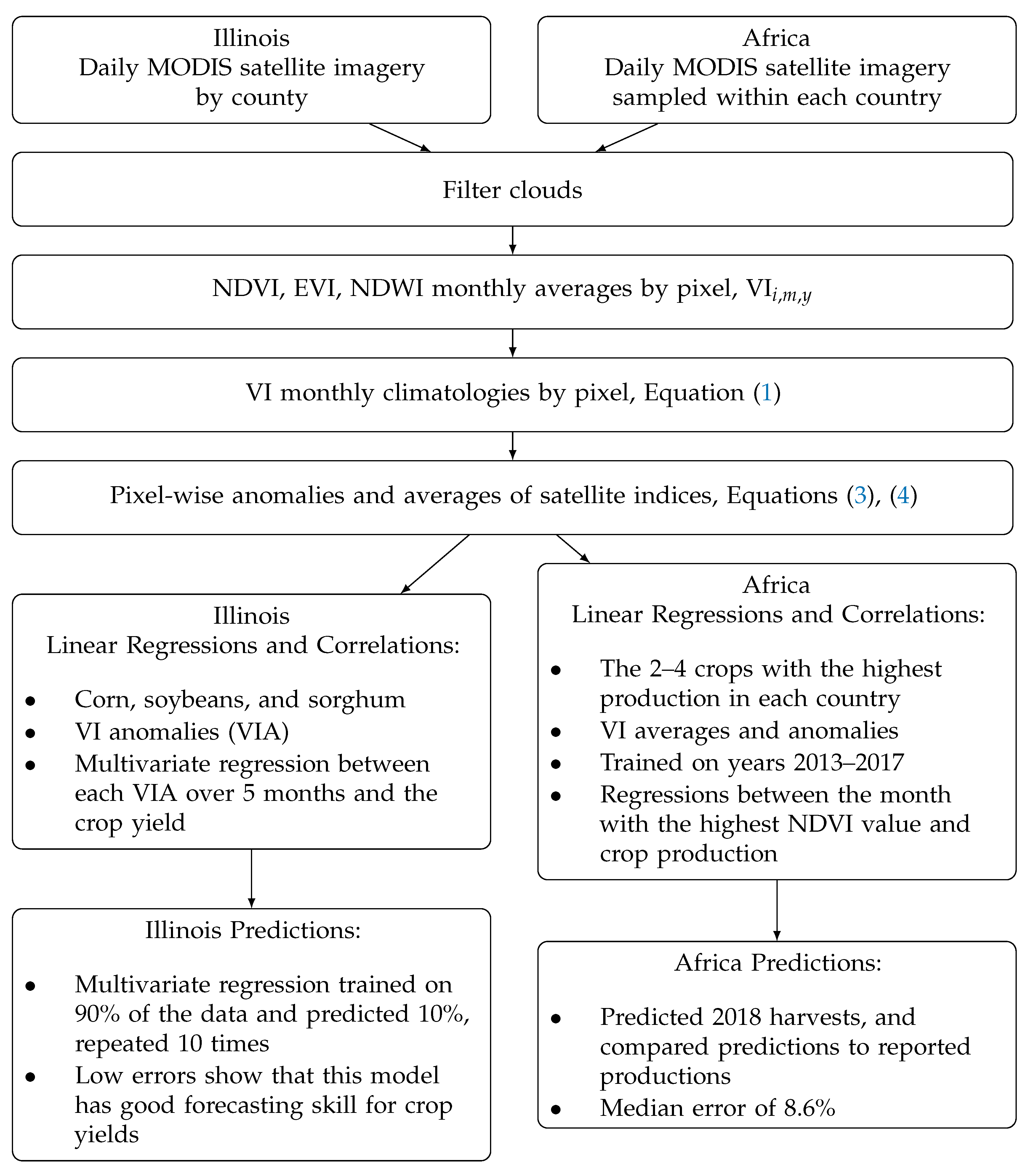
The primary goal of this research is to create a predictive measure of crop yields computed from satellite data. Python code was written to obtain satellite images, mask out clouds, calculate vegetation and water indices (VI), compute monthly VI anomalies since 2000, and correlate the anomalies with crop yield anomalies for every county in Illinois, which served as a proof of concept due to large amounts of ground truth data in the US. The same method was then applied to every country in Africa to create an early indicator of crop yields. The overall workflow is diagrammed in Figure 2 and is described in detail in this section.

Moderate Resolution Imaging Spectroradiometer (MODIS) imagery was obtained from the Descartes Labs Satellite Platform (Figure 3a,b). MODIS, hosted on the satellites Aqua and Terra, has a revisit time of one day, giving almost continuous imagery across the entire earth since 2000. I interacted with the Descartes Labs Satellite Platform through a python console on a laptop computer. Data from MODIS have a nominal resolution of 250 m at the nadir of each swath. In the Descartes Platform, MOD09 Aqua and Terra surface reflectance data points with associated coordinates are interpolated onto a grid in the form of an image [47]. The python code then sends a request to the platform to retrieve a band over a certain area and satellite pass (e.g., green band over an Illinois county for 1 January 2017). The MODIS data were obtained in early 2018. The rest of the analysis was done in the code, which is posted on Github [48].

Clouds, snow and poor atmospheric conditions in images can disrupt data and distort values. To account for cloud contamination, the standard MODIS cloud mask was retrieved from the Descartes Platform. Pixels with clouds or snow were not included in monthly averages, and images with over 80% clouds were removed altogether (Figure 3c).

To measure the health of crops throughout the growing season, three VIs were computed: Normalized Difference Vegetation Index (NDVI), Enhanced Vegetation Index (EVI), and Normalized Difference Water Index (NDWI) [49] (

Table 1. Definitions of vegetation indices to measure crop health. NIR is near infrared; G is the gain factor; L is the canopy background adjustment that addresses non-linear, differential NIR and red radiant transfer through a canopy; and $C_1$ and $C2$ are the coefficients of the aerosol resistance term, which uses the blue band to correct for aerosol influences in the red band.

Index	Description	Formula
NDVI	Normalized Difference Vegetation Index	$\mathrm{NDVI}={\displaystyle \frac{\mathrm{NIR}-\mathrm{Red}}{\mathrm{NIR}+\mathrm{Red}}}$
EVI	Enhanced Vegetation Index	$\mathrm{EVI}=G\ast {\displaystyle \frac{\mathrm{NIR}-\mathrm{Red}}{\mathrm{NIR}+C_1\ast \mathrm{Red}-C2\ast \mathrm{Blue}+L}}$
NDWI	Normalized Difference Water Index	$\mathrm{NDWI}={\displaystyle \frac{\mathrm{Green}-\mathrm{NIR}}{\mathrm{Green}+\mathrm{NIR}}}$

). All three indices have served as crop monitoring tools in previous studies, and have been shown to resemble actual crop conditions [37,50,51]. The indices range from −1 to 1. Areas containing dense vegetation show high NDVI and EVI values (between 0.4 and 0.8), desert sands will register at about zero, and snow and clouds are negative. All of these VIs are sensitive to the same biophysical variables (LAI, leaf angle, soil brightness, chlorophyll content, etc.). Although the indices are similar, it is valuable to examine all three, as they may perform differently under various environmental conditions [52,53,54].

For every pixel in Illinois, the VI monthly averages and climatologies were computed. The process begins with daily cloud-masked MODIS swaths (Figure 3). The monthly average of a vegetative index (NDVI, EVI, and NDWI) is written as ${\mathrm{VI}}_{i,m,y}$, where the subscripts are pixel, month, and year indices. Monthly averaging was chosen for simplicity. VI metrics are defined as follows.

$$\begin{array}{cc}\hfill \text{VI climatology per pixel}:\hspace{1em}{\overline{\mathrm{VI}}}_{i,m}^y& =\frac{1}{N_y}\sum _{y=1}^{N_y}{\mathrm{VI}}_{i,m,y}\hfill \end{array}$$

(1)

$$\begin{array}{cc}\hfill \text{VI anomaly per pixel}:\hspace{1em}{\mathrm{VIA}}_{i,m,y}& ={\mathrm{VI}}_{i,m,y}-{\overline{\mathrm{VI}}}_{i,m}^y\hfill \end{array}$$

(2)

$$\begin{array}{cc}\hfill \text{VI anomaly}:\hspace{1em}{\overline{\mathrm{VIA}}}_{m,y}^i& =\frac{1}{N_i}\sum _{i=1}^{N_i}{\mathrm{VIA}}_{i,m,y}\hfill \end{array}$$

(3)

$$\begin{array}{cc}\hfill \text{VI average}:\hspace{1em}{\overline{\mathrm{VI}}}_{m,y}^i& =\frac{1}{N_i}\sum _{i=1}^{N_i}{\mathrm{VI}}_{i,m,y}\hfill \end{array}$$

(4)

where ${\overline{(·)}}^y$ indicates an average over years, ${\overline{(·)}}^i$ is a spatial average over pixels, and VIA is the vegetative index anomaly. For Illinois, the climatology is defined as the average VI over 2000–2016 for each month and pixel (Equation (1)). Next, the monthly climatology is subtracted from the monthly average for every pixel, resulting in the monthly anomaly (Equation (2)). The pixels in each county are averaged together to find the county-wide monthly anomaly (Equation (3)) and county-wide monthly average (Equation (4)). Figure 4 shows examples of the NDVI monthly average and climatology for Pike County, Illinois. The difference between a dry year and a wet year can be clearly seen in comparison to the climatology.

Illinois was chosen as a test site because the land is mostly agricultural and can provide a clear signal of crop health. Illinois also has very little irrigation: most counties irrigate less than 1% of their fields [55]. Similarly, 90% of staple food production in sub-Saharan Africa comes from rain-fed farming systems [56].

Annual crop yield data was downloaded for every county in Illinois for 2000–2016 for three crops, corn, soybeans, and sorghum, from USDA county estimate reports available online through Quickstats [1]. These crops were chosen because they are three of the largest food crops in Illinois with 4.5 million, 4.3 million, and 7.3 thousands hectares planted, respectively [57,58,59]. Because each county has different growing conditions (soil quality, hills, proximity to large water bodies, etc.), the mean was subtracted out of each county’s crop yield to find the yield anomaly,

$$\begin{array}{c}\hfill \mathrm{Yield} {\mathrm{Anom}}_{i,y}={\mathrm{Yield}}_{i,y}-{\overline{\mathrm{Yield}}}_i^y\end{array}$$

(5)

so that comparisons could be made across all counties. Correlations were found between each county’s yield anomaly and the three VIs for five months, May–September. To find the highest possible correlation amongst these variables and months, a multivariate regression was fit to each month and index for a total of 15 variables (5 months × 3 VIs).

To test the predictive ability of the model, the data were split into a training group of 90% and a testing group of the remaining 10%. The multivariate regression was then fit to the training data and asked to predict the testing set. To ensure randomness, this process was repeated ten times for each crop, and the analysis is the composite of these ten prediction sets.

After testing in Illinois was complete, the method was applied to three countries in Africa: Ethiopia, Tunisia, and Morocco. These countries were used as initial case studies because they have a recent history of relative agricultural and political stability and offer a range of climates and crops. In each country, the two to four highest-producing crops were analyzed. African crop yields were downloaded from Index Mundi, a comprehensive data portal with country-level statistics compiled from multiple sources, but the production data were originally collected by the USDA Foreign Agricultural Service (FAS) [60].

In each country, a box was analyzed over a dense farming region, which served as a representative sample of the entire country. The VI anomalies and averages from these regions were then correlated to national crop production data [60]. Subsections in each country were positioned over areas with the highest local production, which was obtained from the Spatial Production Allocation Model (MAPSPAM) [61]. Sample areas were selected rather than the entire country to limit the amount of data required. A continent-wide analysis would require significant data transfer and computational power, which is expensive and time consuming. Even with subnational sample areas, the MODIS imagery over Africa totaled to 10 terabytes of data. Imagery is only analyzed over dense farming regions to increase simplicity and decrease the amount of data. The full coordinates of every box can be found at [62].

The daily MODIS imagery over the selected boxes in each country was processed in a similar way to Illinois. First, the bands were retrieved from the Descartes Platform. NDVI, EVI, and NDWI were computed, and cloudy pixels were masked out. The climatology for each pixel was subtracted to obtain monthly anomalies as well as averages of all three indices, resulting six variables for correlation analysis: NDVI average, NDVI anomaly, EVI average, EVI anomaly, NDWI average, and NDWI anomaly (Equations (1)–(4)). Next, correlations were computed between the six indices of the month at the height of the growing season and the crop production. The height of the growing season is defined as the month in the growing season that the NDVI average peaks.

After initial successes in Ethiopia, Tunisia, and Morocco, the method was expanded to every African country with the exceptions of Western Sahara, Equatorial Guinea, and Gabon due to lack of crops or constant cloud cover. Satellite data were restricted in this study to 2013–2018 based on the limited download and compute time that is available to a typical home user on a modern-day laptop. The satellite imagery processed in Africa totaled 10 terabytes even with only five years of data. Future production was then predicted for every African country with a harvest between December 2017 (e.g., Ethiopia) and June 2018 (e.g., Namibia). Harvest dates were obtained from the FAO’s GIEWS [63]. Later, once actual production values were published, the error of the predictions in every country and crop was computed. The error is defined as

$${\mathrm{Error}}_j=100\ast ∥\frac{{\mathrm{P}}_j-{\mathrm{A}}_j}{{\mathrm{A}}_j}∥$$

(6)

where P is the predicted yield, A is the reported yield, and j is an index over each county or region.

3. Results

The method was first validated in Illinois and then applied in Africa.

3.1. Illinois

Correlations were computed in Illinois between the anomalies of NDVI, EVI, and NDWI, and three crops: corn, soybeans, and sorghum; all were found to have high correlations. The method was first tested with state-wide averages to show that results are significant when analyzing a large area. The correlations between state-wide corn yield and NDVI, EVI, and NDWI anomalies are extremely statistically significant at $0.90$, $0.85$, and $-0.92$ respectively (Figure 5). It was found that NDVI and EVI both have positive relationships to crop yields, while NDWI is inversely related. This is because the NDWI formulation includes a negative NIR, while NDVI and EVI have positive NIR values.

The central United States was hit by a drought in 2012. During that year, Illinois had lower than average crop yields and a negative NDVI anomaly. Crop yields and NDVI anomalies were significantly higher in 2014, a wet year. These two years are used as examples to show corn yield and satellite anomalies at the county level (Figure 6).

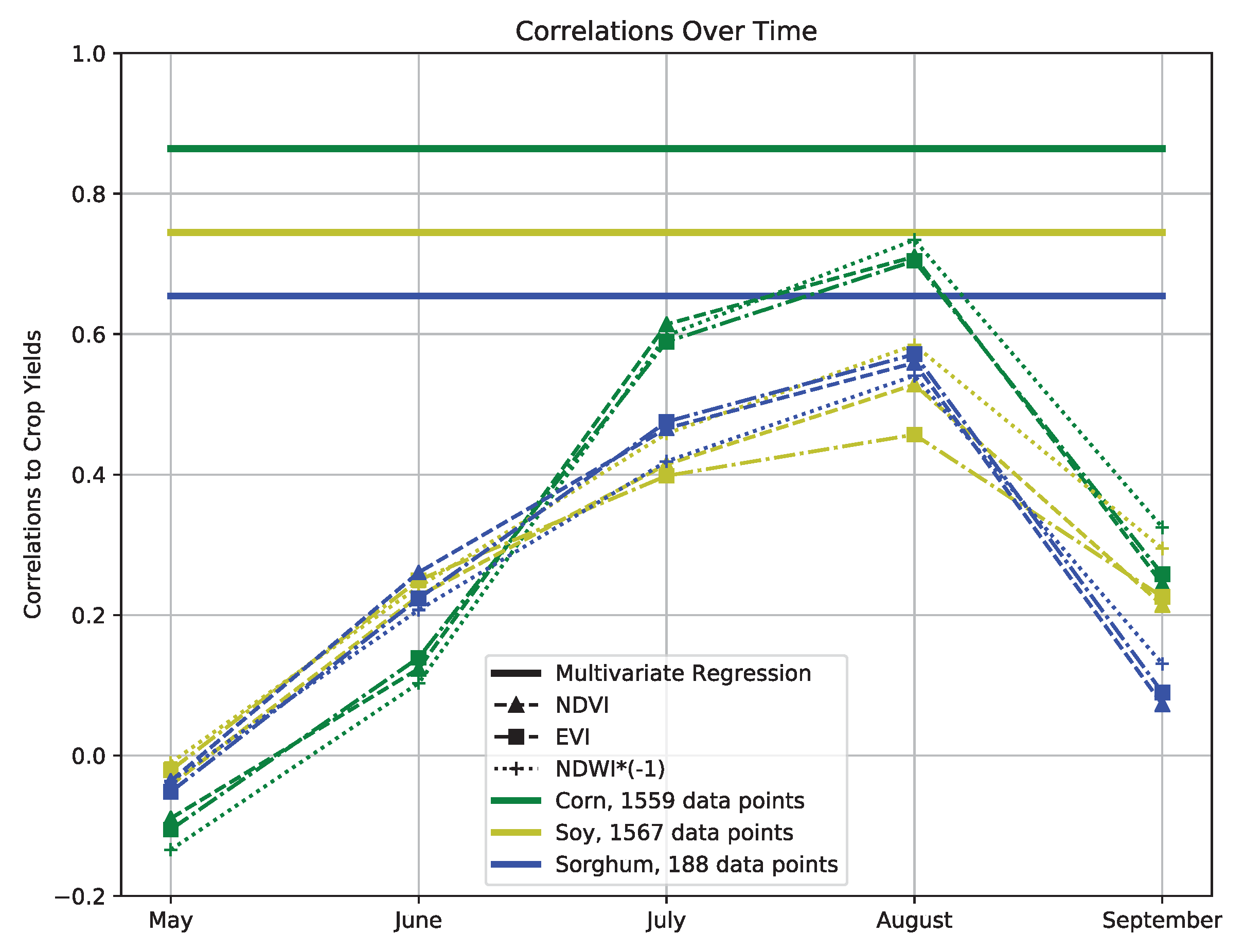
Next, the relationships were examined at a higher resolution. The corn, soybean, and sorghum county yield data were plotted against VI anomalies for every month (May–September), county, and year (2000–2017), for a total of about 1600 data points. August was found to have the highest correlation to all three crops, while July was just slightly lower (Figure 7). Since crops are harvested in October [64], there is a two to three month lead time on yield estimates. Corn had the strongest relation to the VIs with correlations of $0.7$, $0.71$, and $-0.73$ for EVI, NDVI, and NDWI, respectively. Soybeans and sorghum had similar correlations to indices, both ranging from $0.53$ to $0.58$. To see all of the correlations in more detail, refer to Figure 8. All of July’s and August’s correlations had a p-value less than ${10}^{-6}$ [65], meaning there is less than one in a million chance of them occurring through a random process.

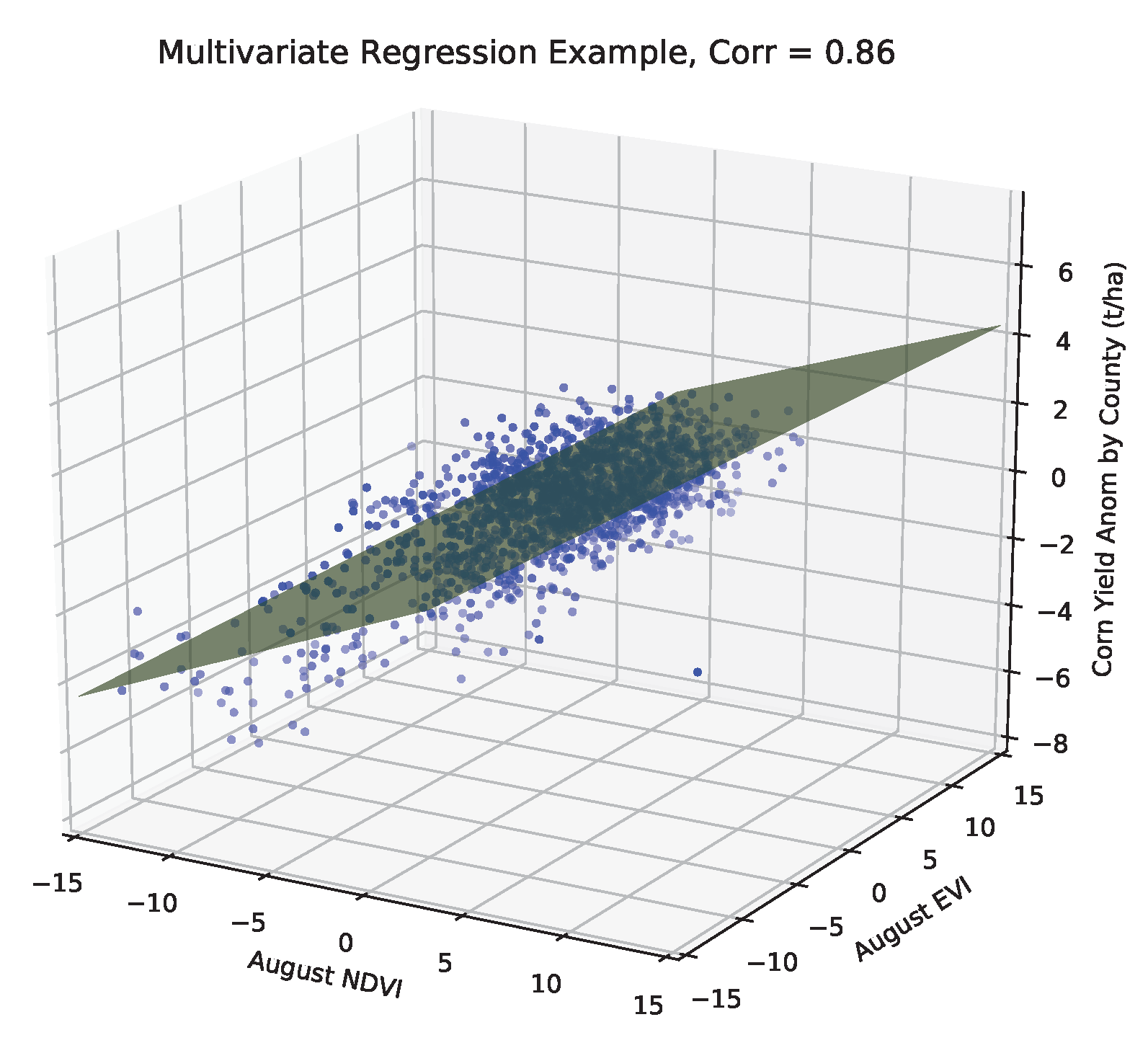
Correlations for each crop have been computed with three indices (NDVI, EVI, and NDWI) and five months, for a total of fifteen independent variables. To create a single predictive measure of crop yields, a multivariate regression was fit to every index and every month using a Python machine learning library. Figure 9 shows an example of the multivariate regression for two of the variables and corn yield. The multivariate regression improved the individual correlations for all three crops to 0.86, 0.74, and 0.65, respectively (solid horizontal lines in Figure 7).

To test the predictive power of the model, the multivariate regression was trained on a random 90% of the data and then predicted the remaining 10%. This process was repeated ten times. The median errors of the predicted yields are 0.56 t/ha (5.7%), 0.18 t/ha (5.8%), and 0.38 t/ha (22%) for corn, soybeans, and sorghum, respectively (Figure 10). The model could predict the yield with reasonable error based on only the VI anomalies of the entire county, demonstrating how this simple method is a good indicator of crop yields.

The error for sorghum is likely higher because it covers a small portion of the state, and no crop mask was used to distinguish the pixels. Corn, soybeans, and sorghum are planted on 4.5 million, 4.3 million, and 7.3 thousands hectares in Illinois, respectively [57,58,59]. While corn and soybeans each cover about a third of the total land in Illinois, sorghum only covers 0.05%. Sorghum fields are therefore a minority of the satellite imagery processed over Illinois. Sorghum in Illinois serves as a proof of concept that a crop can be moderately well predicted even if it only covers a small portion of land.

3.2. Africa

The high correlations in Illinois show that this model has good forecasting skill for crop yields. Next, this method was applied to three countries in Africa: Ethiopia, Morocco, and Tunisia. For each country, a box within a major crop-growing region was analyzed (Figure 11 and Figure 12a). Since the empirical model proposed here uses imagery over the subregion to predict production of the entire country, it implicitly assumes that the vegetation conditions inside the box correspond with those outside the box. This assumption appears to hold true, as correlations over Africa are reasonably high.

Crop estimation in developing countries is vastly different than Illinois and the developed world. The greatest distinctions include the heterogeneity of the landscape, lack of agricultural technology, the spatial size of crop reports, and the accuracy of reported values. In Illinois, the ground is covered with large fields that grow a small number of crops: mostly corn and soybeans. In Africa, the landscape is highly diverse, with small family-owned farms intermixed with villages, lakes, mountains, and forests (Figure 1). These farms, usually much smaller than a hectare, lack much of agricultural technology found in the US, such as pesticides, herbicides, and fertilizers. This makes crops yields much more variable in Africa, both seasonally and spatially. Crop production statistics in Africa are typically only published as a national total. Very rarely are yield or production values reported at the municipality or even state levels. For this reason, crop production was predicted for each country rather than at finer spatial scales, as in the US.

In most regions in Africa, there are wet and dry seasons. For example, the wet season in Ethiopia spans from June to September, and crops are harvested in December. This is known as the Meher growing season. Ethiopia’s core agriculture and food economy is comprised of five major cereals: corn, teff, wheat, sorghum, and barley. These cereals accounted for about three-quarters of total area cultivated and 29 percent of the agricultural GDP during 2005–2006 [66].

The wet and dry seasons are evident in the monthly NDVI values for all three countries (Figure 13). During the wet season, the crops green and the NDVI values spike. During the harvest, the VIs drop. The crops with the highest production in each country were evaluated for this study.

Table A1. The correlations, predictions, and errors for select African countries for every crop and satellite index. All the countries that had harvests between December 2017 and June 2018 are displayed. Forty percent of the predictions had an error of less than 5% from the actual production. The fourth column is correlation between the index and reported crop production from 2013 to 2017.

Country	Crop	Index	Correlation	2018 Predicted (GT)	2018 Actual (GT)	% Error
Botswana	Corn	NDVI Avg	0.984	4	10	61.7
Botswana	Corn	EVI Avg	0.989	3	10	69.1
Botswana	Corn	NDWI Avg	−0.879	0	10	104.9
Botswana	Corn	NDVI Anom	0.893	0	10	100.0
Botswana	Corn	EVI Anom	0.783	0	10	100.0
Botswana	Corn	NDWI Anom	−0.661	0	10	100.0
Botswana	Sorghum	NDVI Avg	0.813	5	8	33.7
Botswana	Sorghum	EVI Avg	0.896	4	8	48.2
Botswana	Sorghum	NDWI Avg	−0.664	3	8	59.0
Botswana	Sorghum	NDVI Anom	0.712	0	8	100.0
Botswana	Sorghum	EVI Anom	0.691	0	8	100.0
Botswana	Sorghum	NDWI Anom	−0.446	0	8	100.0
Burundi	Coffee	NDVI Avg	0.398	172	200	14.1
Burundi	Coffee	EVI Avg	−0.512	226	200	12.8
Burundi	Coffee	NDWI Avg	0.775	202	200	1.2
Burundi	Coffee	NDVI Anom	−0.819	267	200	33.5
Burundi	Coffee	EVI Anom	0.080	202	200	1.0
Burundi	Coffee	NDWI Anom	0.919	210	200	4.8
Burundi	Corn	NDVI Avg	−0.780	170	150	13.2
Burundi	Corn	EVI Avg	0.116	144	150	3.9
Burundi	Corn	NDWI Avg	0.083	146	150	2.7
Burundi	Corn	NDVI Anom	−0.460	159	150	6.2
Burundi	Corn	EVI Anom	0.673	139	150	7.0
Burundi	Corn	NDWI Anom	0.404	147	150	2.1
Burundi	Sorghum	NDVI Avg	−0.594	36	35	3.8
Burundi	Sorghum	EVI Avg	−0.069	30	35	14.3
Burundi	Sorghum	NDWI Avg	−0.033	30	35	15.4
Burundi	Sorghum	NDVI Anom	−0.508	35	35	0.2
Burundi	Sorghum	EVI Anom	0.703	27	35	22.6
Burundi	Sorghum	NDWI Anom	0.296	30	35	14.7
Chad	Corn	NDVI Avg	0.533	457	450	1.5
Chad	Corn	EVI Avg	0.779	437	450	2.8
Chad	Corn	NDWI Avg	−0.037	398	450	11.6
Chad	Corn	NDVI Anom	0.738	284	450	37.0
Chad	Corn	EVI Anom	0.780	275	450	38.8
Chad	Corn	NDWI Anom	−0.713	254	450	43.6
Chad	Millet	NDVI Avg	0.416	705	700	0.8
Chad	Millet	EVI Avg	0.315	680	700	2.9
Chad	Millet	NDWI Avg	−0.297	690	700	1.4
Chad	Millet	NDVI Anom	−0.307	703	700	0.5
Chad	Millet	EVI Anom	−0.241	696	700	0.6
Chad	Millet	NDWI Anom	0.261	708	700	1.1
Chad	Rice	NDVI Avg	0.087	161	154	4.8
Chad	Rice	EVI Avg	−0.251	155	154	0.7
Chad	Rice	NDWI Avg	−0.414	170	154	10.2
Chad	Rice	NDVI Anom	−0.919	195	154	26.5
Chad	Rice	EVI Anom	−0.882	194	154	26.0
Chad	Rice	NDWI Anom	0.800	200	154	29.9
Chad	Sorghum	NDVI Avg	0.562	1433	950	50.8
Chad	Sorghum	EVI Avg	0.735	1340	950	41.0
Chad	Sorghum	NDWI Avg	−0.314	1307	950	37.5
Chad	Sorghum	NDVI Anom	0.842	714	950	24.9
Chad	Sorghum	EVI Anom	0.854	699	950	26.5
Chad	Sorghum	NDWI Anom	−0.959	480	950	49.5
Djibouti	Cereals	NDVI Avg	−0.206	19,185	19,079	0.6
Djibouti	Cereals	EVI Avg	−0.622	18,929	19,079	0.8
Djibouti	Cereals	NDWI Avg	−0.568	19,036	19,079	0.2
Djibouti	Cereals	NDVI Anom	−0.647	18,972	19,079	0.6
Djibouti	Cereals	EVI Anom	−0.668	18,926	19,079	0.8
Djibouti	Cereals	NDWI Anom	0.624	19,056	19,079	0.1
DR Congo	Coffee	NDVI Avg	−0.454	235	220	6.7
DR Congo	Coffee	EVI Avg	−0.453	228	220	3.8
DR Congo	Coffee	NDWI Avg	0.447	232	220	5.5
DR Congo	Coffee	NDVI Anom	−0.188	230	220	4.7
DR Congo	Coffee	EVI Anom	−0.478	201	220	8.4
DR Congo	Coffee	NDWI Anom	0.330	231	220	5.2
DR Congo	Corn	NDVI Avg	0.654	1175	1200	2.1
DR Congo	Corn	EVI Avg	0.652	1190	1200	0.9
DR Congo	Corn	NDWI Avg	−0.522	1183	1200	1.4
DR Congo	Corn	NDVI Anom	0.325	1184	1200	1.3
DR Congo	Corn	EVI Anom	0.348	1221	1200	1.8
DR Congo	Corn	NDWI Anom	−0.434	1183	1200	1.4
Eritrea	Barley	NDVI Avg	−0.191	63	65	3.6
Eritrea	Barley	EVI Avg	−0.252	64	65	2.0
Eritrea	Barley	NDWI Avg	0.142	62	65	4.1
Eritrea	Barley	NDVI Anom	−0.197	63	65	3.6
Eritrea	Barley	EVI Anom	−0.255	64	65	2.1
Eritrea	Barley	NDWI Anom	0.149	62	65	4.1
Eritrea	Millet	NDVI Avg	0.191	25	25	1.3
Eritrea	Millet	EVI Avg	0.252	25	25	0.7
Eritrea	Millet	NDWI Avg	−0.142	25	25	1.4
Eritrea	Millet	NDVI Anom	0.197	25	25	1.3
Eritrea	Millet	EVI Anom	0.255	25	25	0.7
Eritrea	Millet	NDWI Anom	−0.149	25	25	1.4
Ethiopia	Corn	NDVI Avg	0.979	7055	7100	0.6
Ethiopia	Corn	EVI Avg	0.972	7157	7100	0.8
Ethiopia	Corn	NDWI Avg	−0.983	7045	7100	0.8
Ethiopia	Corn	NDVI Anom	0.812	6294	7100	11.4
Ethiopia	Corn	EVI Anom	0.263	6805	7100	4.2
Ethiopia	Corn	NDWI Anom	−0.845	6160	7100	13.2
Ethiopia	Sorghum	NDVI Avg	0.987	4174	4100	1.8
Ethiopia	Sorghum	EVI Avg	0.980	4257	4100	3.8
Ethiopia	Sorghum	NDWI Avg	−0.974	4161	4100	1.5
Ethiopia	Sorghum	NDVI Anom	0.883	3524	4100	14.1
Ethiopia	Sorghum	EVI Anom	0.402	4005	4100	2.3
Ethiopia	Sorghum	NDWI Anom	−0.909	3411	4100	16.8
Guinea-Bissau	Rice	NDVI Avg	0.897	100	99	1.2
Guinea-Bissau	Rice	EVI Avg	0.578	147	99	48.9
Guinea-Bissau	Rice	NDWI Avg	−0.919	91	99	7.9
Guinea-Bissau	Rice	NDVI Anom	0.950	88	99	11.0
Guinea-Bissau	Rice	EVI Anom	−0.446	103	99	3.9
Guinea-Bissau	Rice	NDWI Anom	−0.943	85	99	13.8
Guinea-Bissau	Sorghum	NDVI Avg	0.987	16	20	18.9
Guinea-Bissau	Sorghum	EVI Avg	0.521	22	20	12.3
Guinea-Bissau	Sorghum	NDWI Avg	−0.992	15	20	25.9
Guinea-Bissau	Sorghum	NDVI Anom	0.973	14	20	27.6
Guinea-Bissau	Sorghum	EVI Anom	−0.710	17	20	17.0
Guinea-Bissau	Sorghum	NDWI Anom	−0.989	14	20	30.0
Lesotho	Corn	NDVI Avg	0.611	125	100	24.7
Lesotho	Corn	EVI Avg	0.636	121	100	20.7
Lesotho	Corn	NDWI Avg	−0.652	106	100	5.9
Lesotho	Corn	NDVI Anom	0.535	101	100	1.1
Lesotho	Corn	EVI Anom	0.534	99	100	1.2
Lesotho	Corn	NDWI Anom	−0.660	72	100	28.0
Lesotho	Wheat	NDVI Avg	0.713	12	12	0.3
Lesotho	Wheat	EVI Avg	0.829	12	12	1.0
Lesotho	Wheat	NDWI Avg	−0.619	10	12	13.2
Lesotho	Wheat	NDVI Anom	0.667	10	12	14.8
Lesotho	Wheat	EVI Anom	0.733	10	12	16.1
Lesotho	Wheat	NDWI Anom	−0.646	8	12	30.8
Libya	Barley	NDVI Avg	0.454	100	100	0.0
Libya	Barley	EVI Avg	0.736	100	100	0.1
Libya	Barley	NDWI Avg	−0.538	100	100	0.3
Libya	Barley	NDVI Anom	0.624	100	100	0.1
Libya	Barley	EVI Anom	0.741	100	100	0.1
Libya	Barley	NDWI Anom	−0.618	100	100	0.4
Libya	Olive Oil	NDVI Avg	−0.860	17	18	5.7
Libya	Olive Oil	EVI Avg	−0.850	17	18	4.7
Libya	Olive Oil	NDWI Avg	0.799	17	18	3.7
Libya	Olive Oil	NDVI Anom	−0.791	17	18	4.9
Libya	Olive Oil	EVI Anom	−0.859	17	18	4.8
Libya	Olive Oil	NDWI Anom	0.776	17	18	3.4
Madagascar	Coffee	NDVI Avg	0.244	392	300	30.9
Madagascar	Coffee	EVI Avg	0.241	403	300	34.5
Madagascar	Coffee	NDWI Avg	−0.467	412	300	37.6
Madagascar	Coffee	NDVI Anom	−0.160	465	300	55.1
Madagascar	Coffee	EVI Anom	0.046	416	300	38.9
Madagascar	Coffee	NDWI Anom	−0.216	406	300	35.5
Madagascar	Corn	NDVI Avg	−0.180	347	300	15.8
Madagascar	Corn	EVI Avg	0.175	339	300	13.0
Madagascar	Corn	NDWI Avg	0.036	342	300	14.2
Madagascar	Corn	NDVI Anom	−0.678	378	300	26.2
Madagascar	Corn	EVI Anom	0.004	342	300	14.1
Madagascar	Corn	NDWI Anom	0.393	349	300	16.5
Madagascar	Rice	NDVI Avg	0.622	2234	2304	3.0
Madagascar	Rice	EVI Avg	0.730	2257	2304	2.0
Madagascar	Rice	NDWI Avg	−0.652	2322	2304	0.8
Madagascar	Rice	NDVI Anom	0.030	2335	2304	1.4
Madagascar	Rice	EVI Anom	0.579	2206	2304	4.2
Madagascar	Rice	NDWI Anom	−0.176	2325	2304	0.9
Madagascar	Sugar	NDVI Avg	0.647	90	90	0.5
Madagascar	Sugar	EVI Avg	0.447	93	90	3.8
Madagascar	Sugar	NDWI Avg	−0.836	94	90	5.1
Madagascar	Sugar	NDVI Anom	0.262	91	90	1.9
Madagascar	Sugar	EVI Anom	0.265	93	90	3.3
Madagascar	Sugar	NDWI Anom	−0.587	92	90	3.1
Malawi	Corn	NDVI Avg	−0.206	3309	3000	10.3
Malawi	Corn	EVI Avg	0.848	2362	3000	21.3
Malawi	Corn	NDWI Avg	0.496	3275	3000	9.2
Malawi	Corn	NDVI Anom	−0.206	3309	3000	10.3
Malawi	Corn	EVI Anom	0.848	2363	3000	21.2
Malawi	Corn	NDWI Anom	0.496	3275	3000	9.2
Malawi	Cotton	NDVI Avg	0.060	121	90	34.6
Malawi	Cotton	EVI Avg	0.474	81	90	9.5
Malawi	Cotton	NDWI Avg	0.107	122	90	35.6
Malawi	Cotton	NDVI Anom	0.061	121	90	34.6
Malawi	Cotton	EVI Anom	0.474	81	90	9.5
Malawi	Cotton	NDWI Anom	0.107	122	90	35.6
Malawi	Peanut Oilseed	NDVI Avg	0.395	292	325	10.1
Malawi	Peanut Oilseed	EVI Avg	−0.028	299	325	7.8
Malawi	Peanut Oilseed	NDWI Avg	−0.375	297	325	8.5
Malawi	Peanut Oilseed	NDVI Anom	0.395	292	325	10.1
Malawi	Peanut Oilseed	EVI Anom	−0.028	299	325	7.8
Malawi	Peanut Oilseed	NDWI Anom	−0.375	297	325	8.5
Morocco	Barley	NDVI Avg	0.524	2014	2500	19.5
Morocco	Barley	EVI Avg	0.473	2496	2500	0.1
Morocco	Barley	NDWI Avg	−0.494	2051	2500	18.0
Morocco	Barley	NDVI Anom	0.504	1851	2500	26.0
Morocco	Barley	EVI Anom	0.534	2430	2500	2.8
Morocco	Barley	NDWI Anom	−0.471	1894	2500	24.2
Morocco	Wheat	NDVI Avg	0.669	5666	8200	30.9
Morocco	Wheat	EVI Avg	0.623	6879	8200	16.1
Morocco	Wheat	NDWI Avg	−0.642	5757	8200	29.8
Morocco	Wheat	NDVI Anom	0.641	5270	8200	35.7
Morocco	Wheat	EVI Anom	0.667	6666	8200	18.7
Morocco	Wheat	NDWI Anom	−0.606	5371	8200	34.5
Namibia	Corn	NDVI Avg	0.643	50	58	14.4
Namibia	Corn	EVI Avg	0.642	48	58	18.0
Namibia	Corn	NDWI Avg	−0.581	48	58	18.0
Namibia	Corn	NDVI Anom	0.808	54	58	6.6
Namibia	Corn	EVI Anom	0.811	56	58	3.9
Namibia	Corn	NDWI Anom	−0.727	48	58	16.8
Nigeria	Corn	NDVI Avg	−0.890	9628	11,000	12.5
Nigeria	Corn	EVI Avg	0.276	11,440	11,000	4.0
Nigeria	Corn	NDWI Avg	0.983	9498	11,000	13.7
Nigeria	Corn	NDVI Anom	0.160	10,178	11,000	7.5
Nigeria	Corn	EVI Anom	0.147	10,355	11,000	5.9
Nigeria	Corn	NDWI Anom	0.217	10,363	11,000	5.8
Nigeria	Rice	NDVI Avg	0.939	3932	3780	4.0
Nigeria	Rice	EVI Avg	−0.226	3704	3780	2.0
Nigeria	Rice	NDWI Avg	−0.961	3941	3780	4.3
Nigeria	Rice	NDVI Anom	−0.343	3885	3780	2.8
Nigeria	Rice	EVI Anom	−0.365	3835	3780	1.5
Nigeria	Rice	NDWI Anom	−0.175	3824	3780	1.2
Nigeria	Sorghum	NDVI Avg	−0.930	5708	6800	16.1
Nigeria	Sorghum	EVI Avg	0.397	7866	6800	15.7
Nigeria	Sorghum	NDWI Avg	0.950	5647	6800	17.0
Nigeria	Sorghum	NDVI Anom	0.095	6339	6800	6.8
Nigeria	Sorghum	EVI Anom	0.132	6425	6800	5.5
Nigeria	Sorghum	NDWI Anom	0.341	6411	6800	5.7
Rwanda	Coffee	NDVI Avg	−0.539	254	250	1.5
Rwanda	Coffee	EVI Avg	0.743	253	250	1.3
Rwanda	Coffee	NDWI Avg	−0.762	311	250	24.3
Rwanda	Coffee	NDVI Anom	0.991	223	250	10.9
Rwanda	Coffee	EVI Anom	0.744	253	250	1.3
Rwanda	Coffee	NDWI Anom	0.063	254	250	1.7
Rwanda	Corn	NDVI Avg	−0.440	576	400	43.9
Rwanda	Corn	EVI Avg	0.425	556	400	39.1
Rwanda	Corn	NDWI Avg	−0.411	574	400	43.5
Rwanda	Corn	NDVI Anom	−0.473	556	400	39.0
Rwanda	Corn	EVI Anom	0.424	556	400	39.1
Rwanda	Corn	NDWI Anom	0.951	551	400	37.8
Rwanda	Sorghum	NDVI Avg	−0.226	146	145	1.0
Rwanda	Sorghum	EVI Avg	−0.541	144	145	0.6
Rwanda	Sorghum	NDWI Avg	0.521	142	145	2.4
Rwanda	Sorghum	NDVI Anom	0.318	143	145	1.2
Rwanda	Sorghum	EVI Anom	−0.541	144	145	0.6
Rwanda	Sorghum	NDWI Anom	−0.981	145	145	0.2
Somalia	Corn	NDVI Avg	0.910	104	100	3.6
Somalia	Corn	EVI Avg	0.243	105	100	4.6
Somalia	Corn	NDWI Avg	−0.365	121	100	21.0
Somalia	Corn	NDVI Anom	0.385	103	100	3.5
Somalia	Corn	EVI Anom	0.243	105	100	4.6
Somalia	Corn	NDWI Anom	−0.420	103	100	3.3
Somalia	Sorghum	NDVI Avg	0.432	116	130	10.7
Somalia	Sorghum	EVI Avg	0.196	122	130	6.0
Somalia	Sorghum	NDWI Avg	−0.128	148	130	14.2
Somalia	Sorghum	NDVI Anom	−0.474	190	130	45.9
Somalia	Sorghum	EVI Anom	0.195	122	130	6.0
Somalia	Sorghum	NDWI Anom	−0.115	123	130	5.2
South Africa	Corn	NDVI Avg	−0.592	7392	13,500	45.2
South Africa	Corn	EVI Avg	−0.673	5684	13,500	57.9
South Africa	Corn	NDWI Avg	0.651	7471	13,500	44.7
South Africa	Corn	NDVI Anom	−0.848	2343	13,500	82.6
South Africa	Corn	EVI Anom	−0.859	1967	13,500	85.4
South Africa	Corn	NDWI Anom	0.902	3006	13,500	77.7
South Africa	Sugar	NDVI Avg	0.366	2283	2200	3.8
South Africa	Sugar	EVI Avg	0.467	2439	2200	10.9
South Africa	Sugar	NDWI Avg	−0.430	2297	2200	4.4
South Africa	Sugar	NDVI Anom	0.343	2384	2200	8.4
South Africa	Sugar	EVI Anom	0.292	2333	2200	6.1
South Africa	Sugar	NDWI Anom	−0.396	2391	2200	8.7
South Africa	Wheat	NDVI Avg	−0.746	1383	1800	23.1
South Africa	Wheat	EVI Avg	−0.778	1310	1800	27.2
South Africa	Wheat	NDWI Avg	0.775	1405	1800	21.9
South Africa	Wheat	NDVI Anom	−0.984	1114	1800	38.1
South Africa	Wheat	EVI Anom	−0.998	1091	1800	39.4
South Africa	Wheat	NDWI Anom	0.995	1179	1800	34.5
Sudan	Cotton	NDVI Avg	−0.849	178	500	64.5
Sudan	Cotton	EVI Avg	−0.776	162	500	67.5
Sudan	Cotton	NDWI Avg	0.971	193	500	61.3
Sudan	Cotton	NDVI Anom	−0.748	172	500	65.7
Sudan	Cotton	EVI Anom	−0.754	161	500	67.8
Sudan	Cotton	NDWI Anom	0.804	175	500	65.0
Sudan	Millet	NDVI Avg	−0.565	1018	1000	1.8
Sudan	Millet	EVI Avg	−0.515	835	1000	16.5
Sudan	Millet	NDWI Avg	0.478	1150	1000	15.0
Sudan	Millet	NDVI Anom	−0.548	941	1000	5.9
Sudan	Millet	EVI Anom	−0.510	820	1000	18.0
Sudan	Millet	NDWI Anom	0.455	989	1000	1.1
Sudan	Sorghum	NDVI Avg	−0.875	4945	4000	23.6
Sudan	Sorghum	EVI Avg	−0.837	3802	4000	4.9
Sudan	Sorghum	NDWI Avg	0.798	5811	4000	45.3
Sudan	Sorghum	NDVI Anom	−0.851	4482	4000	12.1
Sudan	Sorghum	EVI Anom	−0.830	3704	4000	7.4
Sudan	Sorghum	NDWI Anom	0.804	4773	4000	19.3
Sudan	Sugar	NDVI Avg	0.340	682	700	2.6
Sudan	Sugar	EVI Avg	0.457	690	700	1.5
Sudan	Sugar	NDWI Avg	−0.025	682	700	2.6
Sudan	Sugar	NDVI Anom	0.484	685	700	2.2
Sudan	Sugar	EVI Anom	0.486	691	700	1.3
Sudan	Sugar	NDWI Anom	−0.425	682	700	2.5
Sudan	Wheat	NDVI Avg	0.239	455	400	13.7
Sudan	Wheat	EVI Avg	0.341	464	400	16.1
Sudan	Wheat	NDWI Avg	−0.083	454	400	13.4
Sudan	Wheat	NDVI Anom	0.330	458	400	14.6
Sudan	Wheat	EVI Anom	0.359	466	400	16.5
Sudan	Wheat	NDWI Anom	−0.364	456	400	14.0
Swaziland	Corn	NDVI Avg	0.917	89	70	27.0
Swaziland	Corn	EVI Avg	0.811	85	70	22.1
Swaziland	Corn	NDWI Avg	−0.950	95	70	36.1
Swaziland	Corn	NDVI Anom	0.826	83	70	18.9
Swaziland	Corn	EVI Anom	0.720	85	70	21.1
Swaziland	Corn	NDWI Anom	−0.853	88	70	25.1
Swaziland	Sugar	NDVI Avg	−0.383	659	690	4.5
Swaziland	Sugar	EVI Avg	−0.214	663	690	4.0
Swaziland	Sugar	NDWI Avg	0.569	650	690	5.8
Swaziland	Sugar	NDVI Anom	−0.278	663	690	3.9
Swaziland	Sugar	EVI Anom	−0.175	663	690	3.9
Swaziland	Sugar	NDWI Anom	0.449	658	690	4.6
Zimbabwe	Corn	NDVI Avg	0.725	931	1700	45.3
Zimbabwe	Corn	EVI Avg	−0.618	1347	1700	20.8
Zimbabwe	Corn	NDWI Avg	−0.816	1022	1700	39.9
Zimbabwe	Corn	NDVI Anom	0.729	934	1700	45.1
Zimbabwe	Corn	EVI Anom	0.212	1268	1700	25.4
Zimbabwe	Corn	NDWI Anom	−0.759	956	1700	43.8
Zimbabwe	Cotton	NDVI Avg	0.897	142	230	38.4
Zimbabwe	Cotton	EVI Avg	−0.029	176	230	23.7
Zimbabwe	Cotton	NDWI Avg	−0.873	158	230	31.2
Zimbabwe	Cotton	NDVI Anom	0.898	142	230	38.1
Zimbabwe	Cotton	EVI Anom	0.346	199	230	13.4
Zimbabwe	Cotton	NDWI Anom	−0.872	148	230	35.8
Zimbabwe	Sugar	NDVI Avg	0.496	448	460	2.6
Zimbabwe	Sugar	EVI Avg	0.236	451	460	1.9
Zimbabwe	Sugar	NDWI Avg	−0.466	452	460	1.8
Zimbabwe	Sugar	NDVI Anom	0.493	448	460	2.5
Zimbabwe	Sugar	EVI Anom	−0.055	453	460	1.5
Zimbabwe	Sugar	NDWI Anom	−0.517	449	460	2.4

in the Appendix A shows the crops examined in each country and the correlation with each satellite index. It was found that Ethiopia and Morocco have the best correlation to the maximum NDVI value of the growing season, while Tunisia has the highest correlations to NDWI.

There was a major drought in Ethiopia in 2015, while 2013 was a very wet year. The vegetation differences can be seen on the pixel level (Figure 12). The anomalies are especially evident in the Rift Valley where farming is most dense.

Ethiopia’s maximum NDVI values, which usually occur in August, are extremely well correlated with grain production at 0.98 and 0.99 for corn and sorghum, respectively (Figure 13a and Figure 14a). That is a near-perfect correlation between the crop production harvested in December and satellite imagery four months earlier. Tunisia and Morocco have correlations of 0.97 and 0.67 to wheat production (Figure 14b,c), showing high predictive skill of satellite indices in all three countries.

3.3. Africa: Prediction of Future Crop Production

After the initial success in Ethiopia, Tunisia, and Morocco, the method was expanded to every African country. First, a box in an agricultural region was selected in each country and a total of 10 terabytes of daily satellite imagery was processed according to the method above. Correlations and linear regressions were computed in every country for their 2–4 highest producing crops. Difficulties in finding accurate correlations include:

• false reporting of production in some countries due to lack of resources, poor oversight, or corruption (e.g., DR Congo, Eritrea, Libya). In severe cases, one could simply use the NDVI anomaly as a proxy for production rather than computing a correlation with reported crop yields, which is commonly done by organizations such as JRC MARS [41];
• multiple growing seasons in specific central countries (Rwanda, Somalia);
• poor quality of earth observation data (e.g., clouds) every day for months at a time in central African countries (Gabon, Cameroon) [31]; and
• time delays and misclassification of harvests during October–December, where production is incorrectly reported in the following calendar year (Nigeria, Sudan).

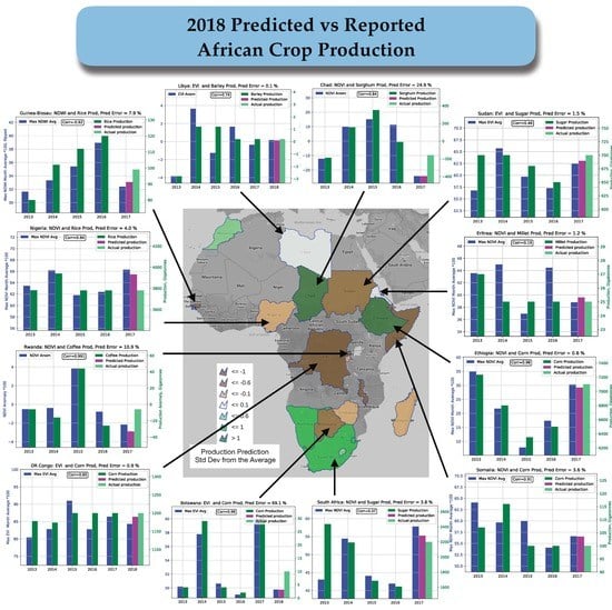
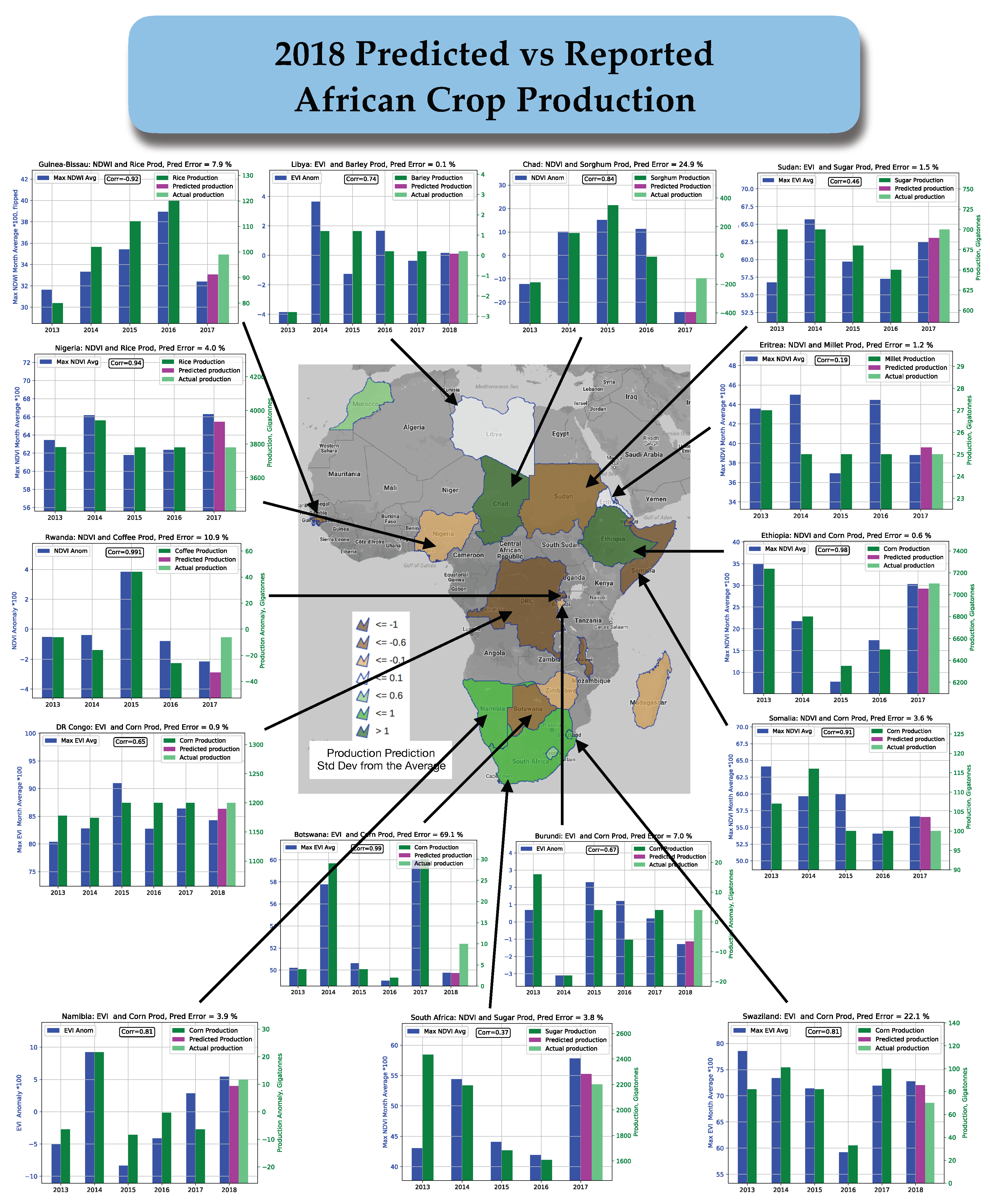
In each African country, correlations were computed between every crop and six indices (NDVI, EVI, NDWI, monthly averages and anomalies). A full listing of all correlations can be found in Table A1 in the Appendix A. Next, the historical regressions were used to predict crop production for 2018 harvests. Every country that reported productions for their 2018 harvest before the publication of this article was examined. This includes harvests ranging from December 2017 (e.g., Ethiopia) through June 2018 (e.g., Namibia), and included a total of 21 countries, about half of Africa. In April 2018, VI anomalies and crop predictions were posted on a publicly viewable interactive map [67], and the actual production values were added as they became available in mid to late 2018 (Figure 15).

In Ethiopia, the model predicted the 2018 harvests to yield 7055 giga-tonnes (GT) of corn and 4174 GT of sorghum. The actual production was 7100 GT and 4100 GT, respectively, for an error of 0.6% and 1.8%. These minimal errors show how this simple model can predict yields very accurately, even with only a few years of historical relationships.

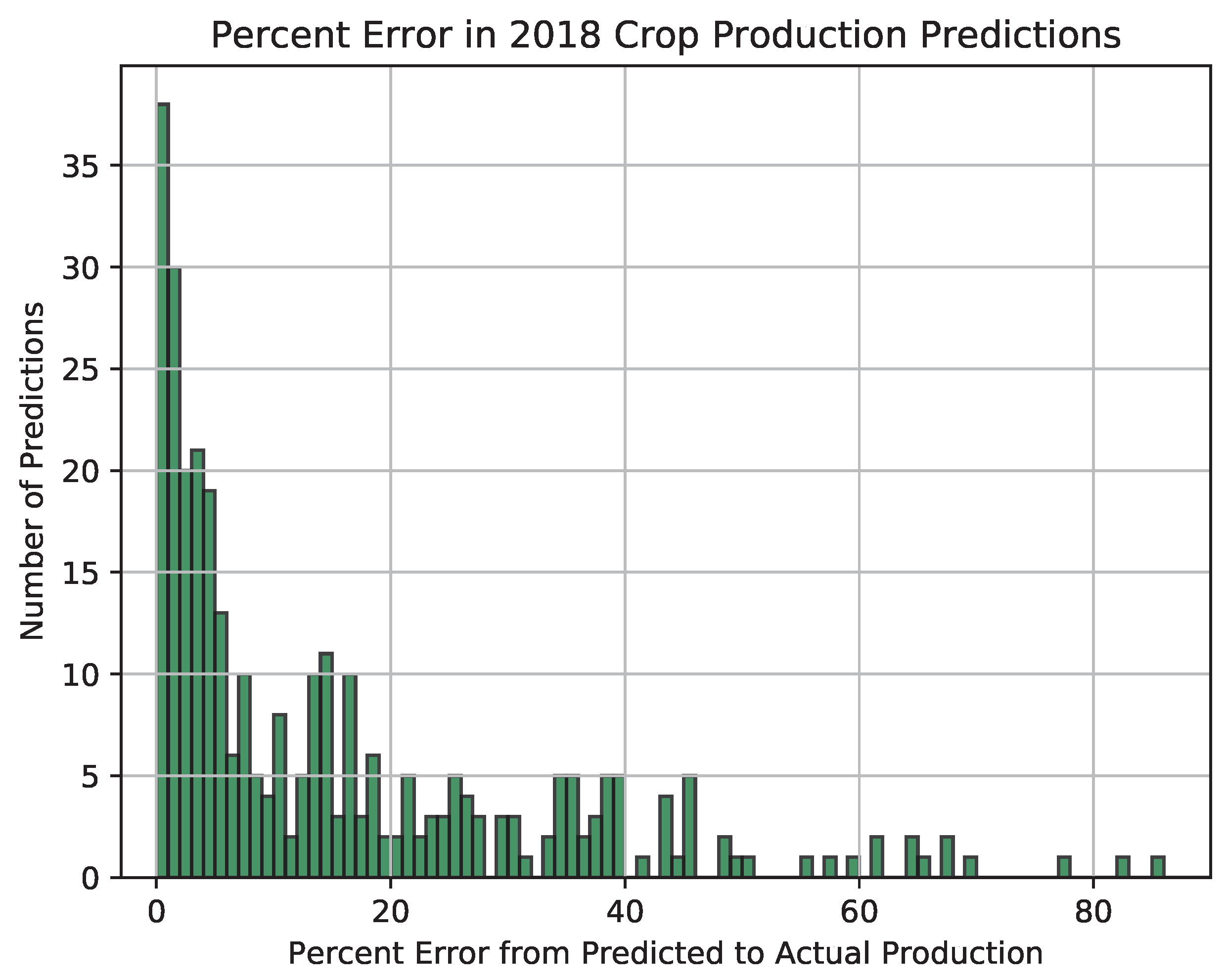
Small errors in predictions were common across Africa. The histogram in Figure 16 displays the percent error for every country, crop, and index. The median error was 8.6%. Twenty-one percent of the predictions had a relative error below 2%, and 40% had errors below 5%.

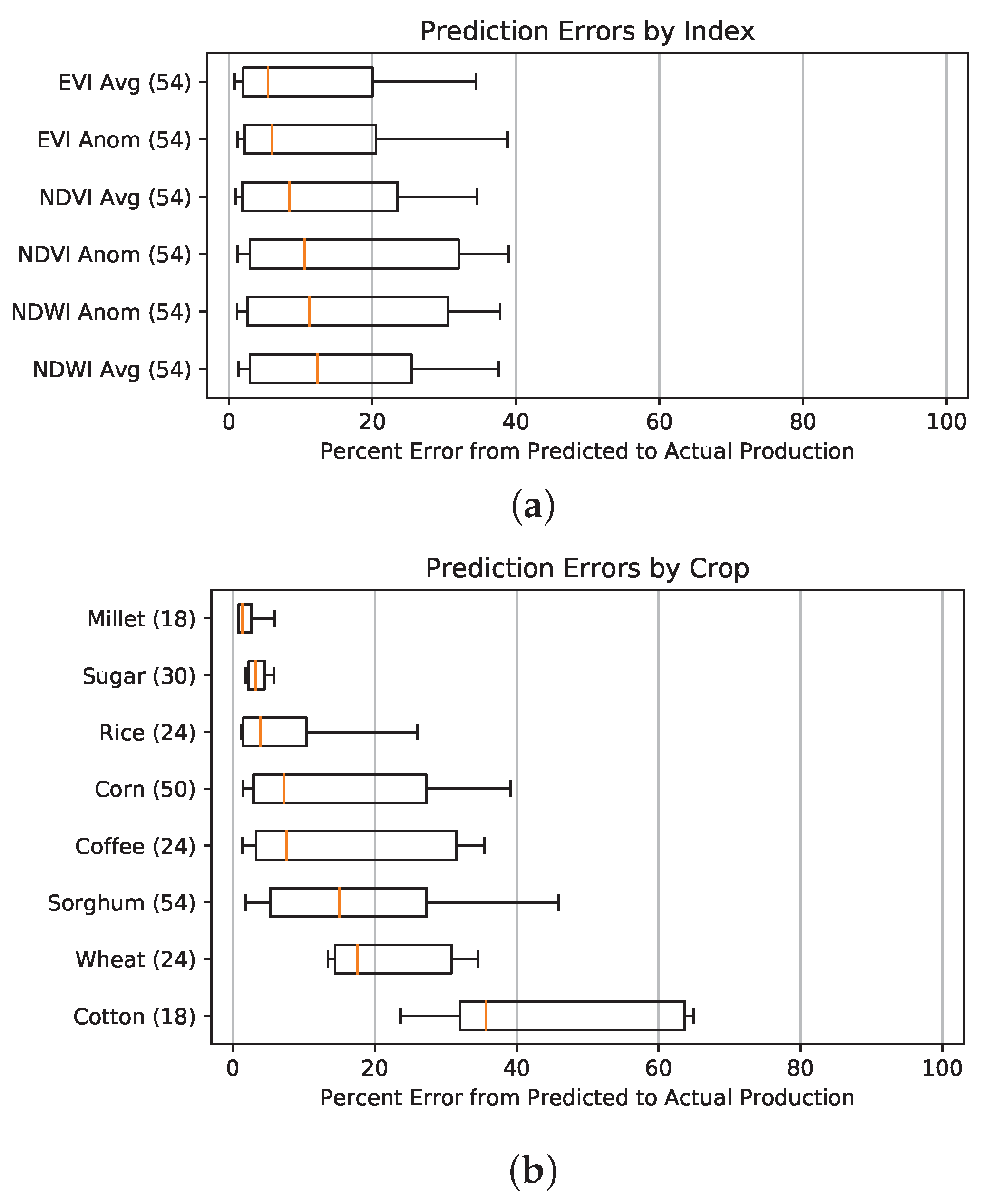
To further examine why some predictions are better than others, the errors were plotted by five groupings: vegetative index, crop, country, latitude, and production anomaly (Figure 17). These categories highlight the factors that contribute to higher errors. For example, cotton, wheat, and sorghum are much harder to predict than millet, sugar, and rice, and extreme years had more error than normal years.

One of the countries with a very high error was Botswana. Botswana’s production of corn and sorghum is very low at only an average of 14 GT, as opposed to Ethiopia’s 4000 GT. In addition, they had a very bad drought year in 2018. With the combination of low production values and a severe drought, the linear regression predicted a negative production. This example displays a drawback of a linear model: In real life, the relationship flattens as yields approach zero, as production cannot actually be negative. However, negative predictions, although not accurate, would still signal alarm in an operational forecast system. In retrospect, flagging Botswana as high risk would have been justified this past year, as they did end up with very low crop production.

4. Conclusions

In this research, I developed a method to predict crop yields 2–4 months before the harvest, based on daily MODIS satellite imagery. The model was first validated in Illinois where there is county-level crop yield data by computing the linear fit between yields and VIs. When a split-sample validation was applied to a multivariate regression with all months of the growing season and all three VIs, the model could predict the crop yields within 5.7%, 5.8%, and 22% for corn, soybeans, and sorghum, respectively. Next, the method was applied to three countries in Africa (Ethiopia, Tunisia, and Morocco), all with different climates and crops. High correlations were found between maximum satellite indices and crop production in all three countries, where sorghum in Ethiopia was the highest at 0.99. After this success, satellite imagery was analyzed in every African country, and productions for the 2018 harvests were predicted 2–4 months before the harvest. Once 2018 harvests were published, the prediction accuracy was tested against the reported values. Forty percent of the predictions were found to have less than a 5% error.

The main objective of this study was to show how a very simple method can serve as an early warning system to predict crop yields in every African country. This method relies solely on NDVI, EVI, and NDWI anomalies calculated over specific subsections of the countries, without the use of crop masks, subnational yield statistics, or special tuning for location or climate. Even with these many simplifications, the model was still able to produce predictions with reasonable error over Illinois and throughout Africa.

The range of prediction errors may be analyzed to better understand the strengths and weaknesses of this model. EVI was able to predict yields most accurately, with NDVI and NDWI following closely (Figure 17a). The averages and anomalies performed similarly. The differences between the indices are within a couple percent, indicating that NDVI, EVI, and NDWI all serve as indirect measures of crop health.

The prediction accuracy for different crops varies substantially. Some crops are harder to predict, as each crop correlates to the VIs with different strengths. Some crops may also be affected by extreme weather late in the season, which this model does not include since it predicts yields from the height during the growing season. Millet, sugar, and rice had the lowest errors, while cotton, wheat, and sorghum were much harder to predict.

Latitude had little influence on prediction errors, indicating that this model can perform in a wide variety of climates (Figure 17d). The southern-most countries performed slightly worse, but these values are likely skewed by Botswana and South Africa, whose large errors are discussed in the previous section and below.

An important part of early warning systems is being able to accurately predict both average and extremely high and low yields. In Figure 17e, it can be seen that extremely good or bad harvests often have greater errors than average harvests. The linear regressions were only trained on five years of data, and were unlikely to experience extreme yields in this short amount of time, meaning the model lacks training data on the tails. To improve the accuracy of the extremes, the model could be trained on more years. However, it is encouraging that the errors are only 15% beyond ±1 std dev, considering the short training period.

A limitation of this model is that it relies on published yield data, so it will not predict as reliably in countries that lack reporting accuracy. In these places, the NDVI anomaly could be used as a proxy for relative crop yields compared to a mean. The model also only predicts yields at the national level and has no subnational component. However, it has the ability to predict yields sub-nationally in the future when sub-national crop data are supplied.

In this study, country-wide crop production was correlated to VI anomalies over dense farming regions to test if small areas could serve as representative samples of the entire country. In most countries, the subregions only covered between 1% and 15% of the total land, depending on the size of the country and box. Despite these small areas, the model produced surprisingly high correlations between the VIs and crop production. South Africa is an exception, with low correlations and high errors in the predictions. South Africa has farms across the country, so the selected box was not able to represent the entire area. In many other African countries, one region is a primary producer and can be used to predict country-wide production.

The model developed here may be compared to the existing early-warning systems of GEOGLAM and FEWS NET. Both are run under large budgets by an extensive team of people with partnerships around the globe. Their systems include local surveyors, remotely sensed data, agroclimate indicators, field reports, and communications with national and regional experts. In contrast, this method can be run by a single user on a modern laptop computer. It was developed over the course of a couple months, and is practically free. This model is also able to predict a numerical value of crop production, while GEOGLAM and FEWS NET present their results as a qualitative measure: conditions are compacted into five categories of crop conditions or food insecurity phases.

The power of the method developed here is that it can be applied to any crop, location, or climate to produce reasonable real-time forecasts of crop yields. It is unique because of its versatility and easy to apply due to its simplicity.

References

- Hamer, H.; Picanso, R.; Prusacki, J.J.; Rater, B.; Johnson, J.; Barnes, K.; Parsons, J.; Young, D.L. USDA/NASS QuickStats US Crop Data. 2017. Available online: https://quickstats.nass.usda.gov (accessed on 30 October 2018).
- Menne, M.J.; Durre, I.; Vose, R.S.; Gleason, B.E.; Houston, T.G. An Overview of the Global Historical Climatology Network-Daily Database. J. Atmos. Ocean. Technol. 2012, 29, 897–910. [Google Scholar] [CrossRef]
- Petersen, L.K. America’s Farming Future: The Impact of Climate Change on Crop Yields. AMS 2018. [Google Scholar] [CrossRef]
- McKinnon, K. GHCN-D: Global Historical Climatology Network Daily Temperatures NCAR—Climate Data Guide. 2016. Available online: https://climatedataguide.ucar.edu/climate-data/ghcn-d-global-historical-climatology-network-daily-temperatures (accessed on 30 October 2018).
- Carletto, G.; Beegle, K.; Himelein, K.; Kilic, T.; Murray, S.; Oseni, M.; Scott, K.; Steele, D. Improving the Availability, Quality and Policy-Relevance of Agricultural Data: The Living Standards Measurement Study Integrated Surveys on Agriculture. In Proceedings of the Third Wye City Group Global Conference on Agricultural and Rural Household Statistic, Washington, DC, USA, 8–9 April 2008; p. 26. [Google Scholar]
- Carletto, C.; Jolliffe, D.; Banerjee, R. From Tragedy to Renaissance: Improving Agricultural Data for Better Policies. J. Dev. Stud. 2015, 51, 133–148. [Google Scholar] [CrossRef]
- Challinor, A.; Wheeler, T.; Garforth, C.; Craufurd, P.; Kassam, A. Assessing the vulnerability of food crop systems in Africa to climate change. Clim. Chang. 2007, 83, 381–399. [Google Scholar] [CrossRef] [Green Version]
- Conceicao, P.; Levine, S.; Lipton, M.; Warren-Rodriguez, A. Toward a food secure future: Ensuring food security for sustainable human development in Sub-Saharan Africa. Food Policy 2016, 60, 1–9. [Google Scholar] [CrossRef]
- The World Bank. World Development Report 2008: Agriculture for Development; The World Bank: Washington, DC, USA, 2008. [Google Scholar]
- Hawkesford, M.J.; Araus, J.L.; Park, R.; Calderini, D.; Miralles, D.; Shen, T.; Zhang, J.; Parry, M.A.J. Prospects of doubling global wheat yields. Food Energy Secur. 2013, 2, 34–48. [Google Scholar] [CrossRef] [Green Version]
- Mann, M.L.; Warner, J.M. Ethiopian wheat yield and yield gap estimation: A spatially explicit small area integrated data approach. Field Crops Res. 2017, 201, 60–74. [Google Scholar] [CrossRef] [PubMed]
- Maas, S.J. Using Satellite Data to Improve Model Estimates of Crop Yield. Agron. J. 1988, 80, 655–662. [Google Scholar] [CrossRef]
- Hellden, U.; Eklundh, L. National Drought Impact Monitoring—A NOAA NDVI and Precipitation Data Study of Ethiopia; Technical Report; Lund University Press: Lund, Sweden, 1988. [Google Scholar]
- Gao, B.C. NDWI—A normalized difference water index for remote sensing of vegetation liquid water from space. Remote Sens. Environ. 1996, 58, 257–266. [Google Scholar] [CrossRef]
- Lobell, D.B. The use of satellite data for crop yield gap analysis. Field Crops Res. 2013, 143, 56–64. [Google Scholar] [CrossRef]
- Johnson, D.M. A comprehensive assessment of the correlations between field crop yields and commonly used MODIS products. Int. J. Appl. Earth Obs. Geoinf. 2016, 52, 65–81. [Google Scholar] [CrossRef] [Green Version]
- Gao, F.; Anderson, M.C.; Zhang, X.; Yang, Z.; Alfieri, J.G.; Kustas, W.P.; Mueller, R.; Johnson, D.M.; Prueger, J.H. Toward mapping crop progress at field scales through fusion of Landsat and MODIS imagery. Remote Sens. Environ. 2017, 188, 9–25. [Google Scholar] [CrossRef]
- Vuolo, F.; Neuwirth, M.; Immitzer, M.; Atzberger, C.; Ng, W.T. How much does multi-temporal Sentinel-2 data improve crop type classification? Int. J. Appl. Earth Obs. Geoinf. 2018, 72, 122–130. [Google Scholar] [CrossRef]
- Jin, Z.; Azzari, G.; Burke, M.; Aston, S.; Lobell, D.B. Mapping Smallholder Yield Heterogeneity at Multiple Scales in Eastern Africa. Remote Sens. 2017, 9, 931. [Google Scholar] [CrossRef]
- Carletto, C.; Gourlay, S.; Winters, P. From Guesstimates to GPStimates: Land Area Measurement and Implications for Agricultural Analysis. J. Afr. Econ. 2015, 24, 593–628. [Google Scholar] [CrossRef] [Green Version]
- United States Department of Agriculture, National Agricultural Statistics Service. Farms and Land in Farms: 2017 Summary. 2018. Available online: http://usda.mannlib.cornell.edu/usda/current/FarmLandIn/FarmLandIn-02-16-2018.pdf (accessed on 30 October 2018).
- Burke, M.; Lobell, D.B. Satellite-based assessment of yield variation and its determinants in smallholder African systems. Proc. Nat. Acad. Sci. USA 2017, 114, 2189–2194. [Google Scholar] [CrossRef] [PubMed] [Green Version]
- Fritz, S.; You, L.; Bun, A.; See, L.; McCallum, I.; Schill, C.; Perger, C.; Liu, J.; Hansen, M.; Obersteiner, M. Cropland for sub-Saharan Africa: A synergistic approach using five land cover data sets. Geophys. Res. Lett. 2011, 38. [Google Scholar] [CrossRef] [Green Version]
- Vancutsem, C.; Pekel, J.; Kayitakire, F. Dynamic mapping of cropland areas in Sub-Saharan Africa using MODIS time series. In Proceedings of the 2011 6th International Workshop on the Analysis of Multi-Temporal Remote Sensing Images (Multi-Temp), Trento, Italy, 12–14 July 2011; pp. 25–28. [Google Scholar]
- Vancutsem, C.; Marinho, E.; Kayitakire, F.; See, L.; Fritz, S.; Vancutsem, C.; Marinho, E.; Kayitakire, F.; See, L.; Fritz, S. Harmonizing and Combining Existing Land Cover/Land Use Datasets for Cropland Area Monitoring at the African Continental Scale. Remote Sens. 2012, 5, 19–41. [Google Scholar] [CrossRef] [Green Version]
- Atzberger, C. Advances in Remote Sensing of Agriculture: Context Description, Existing Operational Monitoring Systems and Major Information Needs. Remote Sens. 2013, 5, 949–981. [Google Scholar] [CrossRef] [Green Version]
- Zhang, X.; Zhang, Q. Monitoring interannual variation in global crop yield using long-term AVHRR and MODIS observations. ISPRS J. Photogram. Remote Sens. 2016, 114, 191–205. [Google Scholar] [CrossRef]
- Tadesse, T.; Senay, G.B.; Berhan, G.; Regassa, T.; Beyene, S. Evaluating a satellite-based seasonal evapotranspiration product and identifying its relationship with other satellite-derived products and crop yield: A case study for Ethiopia. Int. J. Appl. Earth Obs. Geoinf. 2015, 40, 39–54. [Google Scholar] [CrossRef]
- Atzberger, C.; Formaggio, A.R.; Shimabukuro, Y.E.; Udelhoven, T.; Mattiuzzi, M.; Sanchez, G.A.; Arai, E. Obtaining crop-specific time profiles of NDVI: The use of unmixing approaches for serving the continuity between SPOT-VGT and PROBA-V time series. Int. J. Remote Sens. 2014, 35, 2615–2638. [Google Scholar] [CrossRef]
- Immitzer, M.; Böck, S.; Einzmann, K.; Vuolo, F.; Pinnel, N.; Wallner, A.; Atzberger, C. Fractional cover mapping of spruce and pine at 1ha resolution combining very high and medium spatial resolution satellite imagery. Remote Sens. Environ. 2018, 204, 690–703. [Google Scholar] [CrossRef]
- Atzberger, C.; Rembold, F. Mapping the Spatial Distribution of Winter Crops at Sub-Pixel Level Using AVHRR NDVI Time Series and Neural Nets. Remote Sens. 2013, 5, 1335–1354. [Google Scholar] [CrossRef] [Green Version]
- Gissila, T.; Black, E.; Grimes, D.I.F.; Slingo, J.M. Seasonal forecasting of the Ethiopian summer rains. Int. J. Climatol. 2004, 24, 1345–1358. [Google Scholar] [CrossRef] [Green Version]
- Tadesse, T.; Demisse, G.B.; Zaitchik, B.; Dinku, T. Satellite-based hybrid drought monitoring tool for prediction of vegetation condition in Eastern Africa: A case study for Ethiopia. Water Resour. Res. 2014, 50, 2176–2190. [Google Scholar] [CrossRef] [Green Version]
- Klisch, A.; Atzberger, C. Operational Drought Monitoring in Kenya Using MODIS NDVI Time Series. Remote Sens. 2016, 8, 267. [Google Scholar] [CrossRef]
- Enenkel, M.; Steiner, C.; Mistelbauer, T.; Dorigo, W.; Wagner, W.; See, L.; Atzberger, C.; Schneider, S.; Rogenhofer, E. A Combined Satellite-Derived Drought Indicator to Support Humanitarian Aid Organizations. Remote Sens. 2016, 8, 340. [Google Scholar] [CrossRef] [Green Version]
- Rembold, F.; Atzberger, C.; Savin, I.; Rojas, O. Using Low Resolution Satellite Imagery for Yield Prediction and Yield Anomaly Detection. Remote Sens. 2013, 5, 1704–1733. [Google Scholar] [CrossRef] [Green Version]
- Becker-Reshef, I.; Justice, C.; Sullivan, M.; Vermote, E.; Tucker, C.; Anyamba, A.; Small, J.; Pak, E.; Masuoka, E.; Schmaltz, J.; et al. Monitoring Global Croplands with Coarse Resolution Earth Observations: The Global Agriculture Monitoring (GLAM) Project. Remote Sens. 2010, 2, 1589–1609. [Google Scholar] [CrossRef] [Green Version]
- Senay, G.; Velpuri, N.; Bohms, S.; Budde, M.; Young, C.; Rowland, J.; Verdin, J. Chapter 9—Drought Monitoring and Assessment: Remote Sensing and Modeling Approaches for the Famine Early Warning Systems Network. In Hydro-Meteorological Hazards, Risks and Disasters; Shroder, J.F., Paron, P., Baldassarre, G.D., Eds.; Elsevier: Boston, MA, USA, 2015; pp. 233–262. [Google Scholar]
- Funk, C.; Verdin, J.P. Real-Time Decision Support Systems: The Famine Early Warning System Network. In Satellite Rainfall Applications for Surface Hydrology; Springer: Dordrecht, The Netherlands, 2010; pp. 295–320. [Google Scholar]
- Molly, E.; Brown, E.B.B. Evaluating the use of remote sensing data in the U.S. Agency for International Development Famine Early Warning Systems Network. J. Appl. Remote Sens. 2012, 6. [Google Scholar] [CrossRef]
- GIEWS—Global Information and Early Warning System Food and Agriculture Organization of the United Nations. Available online: http://www.fao.org/giews (accessed on 30 October 2018).
- Baruth, B.; Royer, A.; Klisch, A.; Genovese, G. The Use of Remote Sensing Within the Mars Crop Yield Monitoring System of the European Commission. In Proceedings of the 21st Congress of the International Society for Photogrammetry and Remote Sensing—ISPRS, Beijing, China, 3–11 July 2008; Volume 27, pp. 935–940. [Google Scholar]
- Monitoring Agricultural ResourceS (MARS). Available online: https://www.eea.europa.eu/data-and-maps/data/external/monitoring-agricultural-resources-mars (accessed on 30 October 2018).
- Wu, B.; Meng, J.; Li, Q.; Yan, N.; Du, X.; Zhang, M. Remote sensing-based global crop monitoring: Experiences with China’s CropWatch system. Int. J. Digit. Earth 2014, 7, 113–137. [Google Scholar] [CrossRef]
- Domenikiotis, C.; Spiliotopoulos, M.; Tsiros, E.; Dalezios, N.R. Early cotton yield assessment by the use of the NOAA/AVHRR derived Vegetation Condition Index (VCI) in Greece. Int. J. Remote Sens. 2004, 25, 2807–2819. [Google Scholar] [CrossRef]
- Patel, N.R.; Anapashsha, R.; Kumar, S.; Saha, S.K.; Dadhwal, V.K. Assessing potential of MODIS derived temperature/vegetation condition index (TVDI) to infer soil moisture status. Int. J. Remote Sens. 2009, 30, 23–39. [Google Scholar] [CrossRef]
- Labs, D. Descartes Labs: Platform. 2018. Available online: https://www.descarteslabs.com/platform.html (accessed on 30 October 2018).
- Petersen, L.K. MODIS Crop Prediction Code Repository. 2018. Original-Date: 2017-08-01T21:19:50Z. Available online: https://github.com/lillianpetersen/CropPredictionFromSatellite2018 (accessed on 30 October 2018).
- McFeeters, S.K. The use of the Normalized Difference Water Index (NDWI) in the delineation of open water features. Int. J. Remote Sens. 1996, 17, 1425–1432. [Google Scholar] [CrossRef]
- Huete, A.; Didan, K.; Miura, T.; Rodriguez, E.P.; Gao, X.; Ferreira, L.G. Overview of the radiometric and biophysical performance of the MODIS vegetation indices. Remote Sens. Environ. 2002, 83, 195–213. [Google Scholar] [CrossRef]
- Chen, P.Y.; Fedosejevs, G.; Tiscareno-LoPez, M.; Arnold, J.G. Assessment of MODIS-EVI, MODIS-NDVI and VEGETATION-NDVI Composite Data Using Agricultural Measurements: An Example at Corn Fields in Western Mexico. Environ. Monit. Assess. 2006, 119, 69–82. [Google Scholar] [CrossRef] [PubMed]
- Bolton, D.K.; Friedl, M.A. Forecasting crop yield using remotely sensed vegetation indices and crop phenology metrics. Agric. For. Meteorol. 2013, 173, 74–84. [Google Scholar] [CrossRef]
- Matsushita, B.; Yang, W.; Chen, J.; Onda, Y.; Qiu, G.; Matsushita, B.; Yang, W.; Chen, J.; Onda, Y.; Qiu, G. Sensitivity of the Enhanced Vegetation Index (EVI) and Normalized Difference Vegetation Index (NDVI) to Topographic Effects: A Case Study in High-density Cypress Forest. Sensors 2007, 7, 2636–2651. [Google Scholar] [CrossRef] [PubMed] [Green Version]
- Xiao, X.; Zhang, Q.; Hollinger, D.; Aber, J.; Moore, B. Modeling Gross Primary Production of an Evergreen Needleleaf Forest Using Modis and Climate Data. Ecol. Appl. 2005, 15, 954–969. [Google Scholar] [CrossRef]
- United States Department of Agriculture, National Agricultural Statistics Service. Farms and Farmland: Numbers, Acreage, Ownership, and Use; United States Department of Agriculture, National Agricultural Statistics Service: Washington, DC, USA, 2014.
- Cooper, P.J.M.; Dimes, J.; Rao, K.P.C.; Shapiro, B.; Shiferaw, B.; Twomlow, S. Coping better with current climatic variability in the rain-fed farming systems of sub-Saharan Africa: An essential first step in adapting to future climate change? Agric. Ecosyst. Environ. 2008, 126, 24–35. [Google Scholar] [CrossRef] [Green Version]
- United States Department of Agriculture, National Agricultural Statistics Service. Illinois Corn County Estimates: Corn Area Planted And Harvested, Yield, and Production by County—Illinois; Department of Agriculture, National Agricultural Statistics Service: Washington, DC, USA, 2017.
- United States Department of Agriculture, National Agricultural Statistics Service. Illinois Corn County Estimates: Soybean Area Planted And Harvested, Yield, and Production by County—Illinois; Department of Agriculture, National Agricultural Statistics Service: Washington, DC, USA, 2017.
- United States Department of Agriculture, National Agricultural Statistics Service. Illinois Corn County Estimates: Sorghum Area Planted and Harvested, Yield, and Production by County—Illinois; Department of Agriculture, National Agricultural Statistics Service: Washington, DC, USA, 2016.
- Mundi, I. Agricultural Production Statistics by Country. 2018. Available online: https://www.indexmundi.com/agriculture (accessed on 30 October 2018).
- You, L.; Wood, S.; Wood-Sichra, U.; Wu, W. Generating global crop distribution maps: From census to grid. Agric. Syst. 2014, 127, 53–60. [Google Scholar] [CrossRef] [Green Version]
- Petersen, L.K. Dense Farming Regions in Each African Country. 2018. Available online: https://gist.github.com/lillianpetersen/6b2227bad0c44d0a9565c717e6f178d3 (accessed on 30 October 2018).
- FAO GIEWS Country Briefs-Home. Available online: http://www.fao.org/giews/countrybrief/ (accessed on 30 October 2018).
- United States Department of Agriculture. Field Crops Usual Planting and Harvesting Dates; Technical Report; United States Department of Agriculture: Washington, DC, USA, 2010.
- GraphPadSoftware. p-Value Calculator. 2018. Available online: https://www.graphpad.com/quickcalcs/pvalue1.cfm (accessed on 30 October 2018).
- Taffesse, A.S. Crop production in Ethiopia. In Food and Agriculture in Ethiopia Progress and Policy Challenges; University of Pennsylvania Press: Philadelphia, PA, USA, 2012; pp. 53–83. [Google Scholar]
- Petersen, L.K. Predicting Food Shortages in Africa from Satellite Imagery. 2018. Available online: https://lillianpetersen.github.io/africa_satellite (accessed on 30 October 2018).
Figure 1.
Farm fields by satellite in Ethiopia and Illinois at the same resolution. In Africa, small farm fields (smaller than a MODIS pixel) and poor ground truth data increase the difficulty of analyzing and predicting crop yields. Images are from Google Maps.
Figure 2.
Workflow diagram.
Figure 3.
Snapshots of two MODIS satellite passes over Pike county, Illinois (a,b); and the cloud mask for the second image (c). Axes labels show MODIS pixels. Daily MODIS imagery was retrieved for every county in Illinois for 2000–2017 from the Descartes Labs Satellite Platform [47].
Figure 4.
August average NDVI for a drought year (a); August average NDVI for a wet year (b); and the NDVI August climatology (c).
Figure 5.
Illinois mean corn yield since 2000 (green) correlated with the anomalies of July and August: NDVI ((a), blue); EVI ((b), blue) and NDWI ((c), blue). Soybeans and sorghum performed similarly. Reported yields are from the USDA [1], and anomalies are computed from daily MODIS imagery using Equations (1)–(4).
Figure 6.
Corn yield (Column 1), NDVI anomaly (Column 2), EVI anomaly (Column 3), and NDWI anomaly (Column 4) by county in Illinois: for the drought year 2012 (a); and for the wet year 2014 (b). During the drought year, there are low yields, low NDVI and EVI anomalies, and high NDWI anomalies, while the wet year is opposite. Soybeans and sorghum performed similarly.
Figure 7.
Correlations for each month between Illinois corn (green), soybean (yellow), and sorghum (blue) yields and the anomalies of NDVI (dashed), EVI (dot-dashed), and NDWI (dotted). Each point represents the correlation for that month between the respective data, and the multivariate regression correlations are represented by the solid horizontal lines. Every regression with corn included 1559 data points, soybeans had 1567 points, and sorghum had 188 points. July and August have the highest predictive skill for all three crops. These crops are harvested in October, meaning there is a two to three month lead time on yield estimates.
Figure 8.
The correlations between the August anomalies of NDVI (left), EVI (middle), and NDWI (right) with corn (top), soybeans (middle), and sorghum (bottom). Each point represents a single county and year. Corn and soybeans have the best correlations, and sorghum is slightly worse, likely because it is grown much less in Illinois than the other crops. All correlations are extremely significant with p-values less than . August was the month with the highest correlations to yields.
Figure 9.
An example of the multivariate regression comprised of all three satellite indices and five months (15 variables total), but here the corn yield is only plotted against August NDVI and NDWI for visualization purposes. The multivariate regression improved the individual correlations for corn to 0.86.
Figure 10.
Accuracy of the multivariate regression predictions of yields in Illinois for corn (a), soybeans (b), and sorghum (b). Each point shows the predicted yield versus the reported yield for a single county and year. The model was trained with a randomly selected 90% of the data and then predicted the other 10%. This process was then repeated ten times to ensure randomness. The median error (Equation (6)) was lowest for corn with 5.7%, soybeans was similar at 5.8%, and sorghum had the worst error with 21.9%.
Figure 11.
A representative area was chosen in the densest agricultural region of each country to reduce download and computation time, making it feasible to predict crop production for the entire continent of Africa on a home laptop computer. The coordinates of each box can be viewed at [62].
Figure 12.
The box examined in Ethiopia (a) and its September NDVI anomalies during a wet year (b) and a dry year (c). The NDVI anomalies are particularly evident in the Rift Valley, where farming is the most dense.
Figure 13.
NDVI monthly average for: Ethiopia (a); Tunisia (b); and Morocco (c). The annual rainy season produces high NDVI values and corresponds to the crop-growing months. To show an example of correlations, Ethiopia includes the corn production as green bars, which has a very high correlation to maximum NDVI at 0.98. Production data were retrieved for every country from Index Mundi [60].
Figure 14.
Vegetation index at the height of the growing season (green) with crop production (blue) for Ethiopia (a), Tunisia (b), and Morocco (c). Ethiopia and Tunisia have significant correlations at 0.99 and 0.97. Morocco has a correlation of 0.67 and a p-value of 0.1. Ethiopia shows an example of the 2018 crop predictions (pink), which was predicted based on the historical regression and was later compared to reported crop production (light green). The error in Ethiopia is very low at 1.8%.
Figure 15.
The map in the center displays the predicted crop production in standard deviations from the average. Only countries with harvests between December 2017 and June 2018 are displayed. Surrounding the map are bar charts of satellite indices (blue), historical crop production (dark green), predicted 2018 crop production (pink), and actual 2018 production (light green). To view the accuracy of predictions for all crops and countries, see Table A1.
Figure 16.
Histogram of the 2018 prediction errors for each crop and country, as shown in Table A1. Forty percent of the predictions are under 5% error, and over half are below 9%.
Figure 17.
The errors of the 2018 predictions examined in five categories: vegetation index (a); crop (b); country (c); latitude (d); and production anomaly (e). Each orange line represents the median error, the boxes represent the ends of the second and third quartiles, and the whiskers show the middle of the first and fourth quartiles. On the vertical axes, the number of samples of each category are in parentheses. A full listing of predictions and errors are in Table A1.