ISAR Autofocus Imaging Algorithm for Maneuvering Targets Based on Phase Retrieval and Gabor Wavelet Transform


1
School of Information Science and Engineering, Yanshan University, Qinhuangdao 066000, China
2
School of Mathematical & Statistical Sciences, The University of Texas Rio Grande Valley, Edinburg, TX 78539, USA
*
Author to whom correspondence should be addressed.
Remote Sens. 2018, 10(11), 1810; https://doi.org/10.3390/rs10111810
Submission received: 29 September 2018
/
Revised: 6 November 2018
/
Accepted: 13 November 2018
/
Published: 15 November 2018
(This article belongs to the Special Issue Radar Imaging Theory, Techniques, and Applications)
Abstract
:The imaging issue of a rotating maneuvering target with a large angle and a high translational speed has been a challenging problem in the area of inverse synthetic aperture radar (ISAR) autofocus imaging, in particular when the target has both radial and angular accelerations. In this paper, on the basis of the phase retrieval algorithm and the Gabor wavelet transform (GWT), we propose a new method for phase error correction. The approach first performs the range compression on ISAR raw data to obtain range profiles, and then carries out the GWT transform as the time-frequency analysis tool for the rotational motion compensation (RMC) requirement. The time-varying terms, caused by rotational motion in the Doppler frequency shift, are able to be eliminated at the selected time frame. Furthermore, the processed backscattered signal is transformed to the one in the frequency domain while applying the phase retrieval to run the translational motion compensation (TMC). Phase retrieval plays an important role in range tracking, because the ISAR echo module is not affected by both radial velocity and the acceleration of the target. Finally, after the removal of both the rotational and translational motion errors, the time-invariant Doppler shift is generated, and radar returned signals from the same scatterer are always kept in the same range cell. Therefore, the unwanted motion effects can be removed by applying this approach to have an autofocused ISAR image of the maneuvering target. Furthermore, the method does not need to estimate any motion parameters of the maneuvering target, which has proven to be very effective for an ideal range–Doppler processing. Experimental and simulation results verify the feasibility of this approach.
1. Introduction
Inverse synthetic aperture radar (ISAR) imaging has been attracting a lot of attention from many radar researchers in recent years [1,2,3]. ISAR imaging technology provides a new way of thinking in automatic aircraft models classification, which is the classification of small boats in littoral environments via polarimetric ISAR and automatic target recognition (ATR) for multiple targets flying in formation [4,5,6]. Different from other imaging systems of the target [7], the main idea of ISAR imaging is to exploit Doppler information of echoes caused by the rotation of targets. In addition, the uncertainty of the maneuvering target increases the difficulty of ISAR imaging, particularly for the aerial targets. These may include the translational motion (mainly reflected in velocity and acceleration), as well as rotational motion, such as yaw (i.e., the rotational motion described in the text), pitch, and roll. When the maneuvering target has the complex motion described above, traditional imaging algorithms are no longer applicable [8]. In order to obtain a focused and clear image, motion compensation procedures have to be employed in ISAR systems.
There are many popular algorithms dedicated to translational motion compensations (TMC), such as the phase gradient autofocusing technique, entropy minimization method, and cross-correlation method [9,10,11]. The above methods are popular among various ISAR TMC techniques. However, these works are mostly based on motion parameter estimation, and the accuracy of them is low. Phase retrieval is a method that has been developed for optical imaging in recent years [12], and it is gradually being applied in more fields. Due to its simple structure, strong anti-interference ability, and high precision, it has attracted much attention [13]. The phase retrieval algorithm calculates the phase distribution of the light field through measuring the intensity distribution of the optical field [14,15]. A researcher [16] introduced the theory of phase retrieval into the ISAR images reconstruction, especially for removing the non-uniform translational motion. Hongyin Shi et al. suggested that the ISAR echo module of the maneuvering target is not affected by its radial motion, that is, phase retrieval can be applied to compensate for the maneuvering target’s translational motion and from the ISAR image [17]. Moreover, the algorithm uses the Fourier magnitudes of signals as an input [18], and it does not need to estimate the target’s motion parameters. However, it should be pointed out that the phase retrieval method has some difficulties of removing the rotational motion effects from the ISAR image. Autofocused images can be obtained only under the condition that the rotation of the target is small for the coherent integration time of the radar; once the rotation angle becomes larger, the phase retrieval algorithm cannot solve the unfavorable effect caused by the rotational motion.
Time-frequency analysis is an effective method in signal analysis. Applying the time-frequency transform to the signal yields the instantaneous time-frequency characteristics of the signal [19,20]. The time-frequency analysis is illustrated by Wang et al. for ISAR motion compensation [21,22], and the adaptive spectrogram proposed by Berizzi et al [23] is employed to select and extract the phase of multiple prominent point scatterers on the target. In some works [24,25], the authors have carefully chosen a short coherent processing interval using the time-frequency analysis. Although this technique can achieve good imaging results, it has a low utilization rate of radar signals, resulting in the decreasing of the cross-range resolution. According to Thomas et al. [26], in order to obtain the sufficient image resolution, the Gabor basis function introduces three signal parameters that allow the components of a target signature to be mapped into a three-dimensional domain (time, range, and frequency). As one of the tools for the time-frequency analysis in ISAR imaging, Gabor wavelet transform (GWT) can obtain higher quality images than those using long integration intervals [27]. Park and Myung [28] have also employed Gabor representation for the improvement of the image smeared by a target with complicated motion. Specifically, Gabor wavelet transform is a kind of window Fourier transform or short-time Fourier transform that can be utilized to replace the traditional Fourier transform to retrieve the Doppler or cross-range information. Therefore, GWT is a very effective method for removing the rotational motion effects from the ISAR image. Based on joint time-frequency transform processing, GWT extracts an ISAR two-dimensional (2-D) range–Doppler image at each frame to eliminate Doppler smearing, and a 2-D range–Doppler image becomes a three-dimensional (3-D) time-range-Doppler cubic image [29]. However, since the shape of the time-frequency window remains unchanged while only the position changes, the intrinsic link between the frequency and the window width is cut off. For non-stationary signals such as radar echoes, GWT has difficulties with providing a narrow time window to handle the high frequencies of the signal to improve the resolution, resulting in hardly obtaining satisfactory results. Therefore, GWT cannot effectively overcome the range drift and range walk induced by the translational motion, making the imaging performance of high-speed targets worse.
After having an in-depth analysis based on the above procedure, in this paper, we propose a new method to overcome the imaging issues of the rotating maneuvering target with a large angle and at high speed. In our method, the GWT is used for rotational motion compensation (RMC) through taking range compression to the backscattered signal. Then, the phase retrieval is used for TMC to accomplish the range alignment and phase correction. At this stage, all of the scatters of the target remain in their range cells, while the time-invariant Doppler shifts of all of the scatters have been produced. For the imaging purpose, selecting a specific moment in the GWT obtains a completely autofocused ISAR image.
The content of this paper is arranged as follows. In Section 2, an analytic model of the echo signal for a maneuvering target is provided. Section 3 briefly introduces RMC based on GWT. In Section 4, we discuss the TMC through the phase retrieval in detail. Experimental results and simulation analysis are presented in Section 5, and conclusions are given in Section 6.
2. The Analytic Model of Echo Signal for a Maneuvering Target
To present a geometric graph of a maneuvering target, let us build the radar coordinate and target coordinate systems as shown in Figure 1, which are rigidly fixed in the body. Meanwhile, another reference coordinate system is introduced to describe the rotation of the maneuvering target. The coordinate system is parallel to the rectangular system , and its origin is usually located at the target center in the target body’s initial state. The target has a translational motion of and a rotational motion of . Moreover, the target contains Q scatters, where is the th point scatterer. The returned baseband signal at from the target can be expressed as:
where is the speed of light, stands for the frequency of the radar waveform, refers to the reflectivity density function with respect to , and is an abbreviation of the distance from the radar to the scatterer . From Figure 1, can approximately be estimated by:
By Taylor expansion, we have:
where is the azimuth angle of the target, assuming that it is equal to zero, and represents the range from the radar to the geometric center of the target. Similarly, is the target’s initial rotation angle, and we can set to facilitate the signal analysis. and are the target’s radial velocity and acceleration, respectively. and denote the target’s angular velocity and angular acceleration, respectively. Thus, the distance from to radar becomes:
If the coherence processing interval is relatively small, we have:
We ignore the terms greater than second-order in the above equation, substituting Equations (3), (6), and (7) for the distance Equation in (5), so it can be rewritten as:
Therefore, the radar backscattered signal from all of the scatterers can then be represented as:
The Doppler shift induced by the target translation and rotation can be obtained by the time derivative of Equation (8):
For ease of analysis, we substitute into Equation (9), and then an approximation of it will yield:
Since the target moves and rotates with non-uniform speeds, the quadratic terms of the Doppler shift are time varying. In order to obtain a complete and focus (range–Doppler) RD image, all of the phase errors should be corrected, and the time-invariant Doppler shifts must be produced. Hence, the next motion compensation will be performed.
3. RMC Based on GWT
It is assumed that the radar transmits continuous bursts of stepped frequency waveform, each containing narrow-band pulses. Within each burst, the center frequency of each successive pulse increases with a constant frequency step .
where is the stepped frequency value for the th transmitted pulse, .
After measuring the baseband echo signals with a pulse repetition rate at time instants , the unprocessed spatial frequency signal of the target can be represented by the complex data that are organized into a 2-D array where represents the time interval between pulses, .
The origin of the target can be regarded as the geometric phase center, because the phase term has no effect on the target imaging. The range compression performs an point inverse Fourier transform () for each of the received frequency signatures as shown:
where represents the operation with respect to . is the range profiles of the radar scattering signal, and each range profile contains range cells. The range profile consists of multiple “peaks” in different range cells, corresponding to the energy distribution of the received signal. Before Gabor wavelet transform is performed on , the definition of the GWT’s mother wavelet function is given first [26]:
The first and second term represent a Gaussian blur function where the shifting factor is the center of the Gaussian window in each frame of the image, and ( is the selected time frame and is pulse repetition frequency). denotes the standard deviation, and it defines the integration time of the ISAR frames. The third is a harmonic function where the Gaussian window modulation parameter is set to be equal to or less than the PRF, and expands around a preselected frequency band. In addition, the number of oscillations within the Gaussian envelope can be adjusted by setting the modulation parameter , which makes GWT more suitable for time-varying signals.
In each of the following sets of simulation experiments, the parameters are set as optimal. Thus, we will get the best time-frequency resolution, because has the smallest time-frequency product. Moreover, the mother wavelet guarantees that each image obtained will have a minimum range walk and range offset distortion due to the target motion. However, in fact, the number of migrations though resolution cells induced by the rotation of the maneuvering target is less than that caused by the translation. Severe migration through range cells (MTRC) will appear in high-speed maneuvering target imaging results, which is not effectively eliminated by GWT.
Using the GWT, the radar data is expressed as follows:
The modulation parameter is continuously adjusted to perform phase compensation on . After this operation, Equation (15) becomes:
here, . represents the Doppler shift after rotational motion compensation, including only the remaining translational component along the range direction, as a function of time , which is discussed in the next section.
As mentioned above, GWT is a short-time Fourier transform, so now, we need to perform GWT on Equation (16):
where , denotes the GWT operation with respect to , and is the convolution operator over . It’s important to note that the Fourier transform () of the Gaussian function is still the Gaussian function. By performing the GWT at each of ’s range cells and along pulses, an time-varying Doppler spectrum is obtained. Next, it is known that there is a total of range cells, so an time-range–Doppler cube can be formed.
At a particular time instant, , one range–Doppler image frame can be extracted from the cubic image. In fact, each image frame represents a complete RD image extracted at a selected time instant, and we can obtain a sequence of 2-D range–Doppler images by time-sampling the image . The process of GWT is shown in Figure 2.
At this stage, GWT decomposes the phase function of the target echo into instantaneous time segments such that time snapshots of the time-varying ISAR image can be constructed. More importantly, GWT removes the rotational motion error for overcoming smearing in the cross-range direction. Of course, when the target’s radial velocity is small, range alignment can be accomplished by applying the GWT. As shown in Figure 2, when the target’s radial velocity is large, GWT does not have a good performance in eliminating the scatters’ range walk.
4. TMC Based on Phase Retrieval
4.1. Phase Retrieval Principle
In the field of optical imaging, the optical detection device can only detect the signal strength or the Fourier modulus, and then, the phase retrieval algorithm is implemented. For a one-dimensional frequency domain signal with phase and amplitude :
where is a spatial coordinate and is a frequency coordinate. In an optical device, only the signal amplitude can be detected and then used to recover the phase , which is the mechanism of phase retrieval. Next, the distribution function can be obtained by performing the inverse Fourier transform on the known signal .
In practical applications, due to the lack of prior information of the phase retrieval, the correctness of the recovery result cannot be ensured when the phase retrieval of the signal is performed; that is, the result is not unique. Performing the phase retrieval with only a known value of the signal’s Fourier amplitude will inevitably create an ambiguity in the phase. To solve this problem, in the phase retrieval iteration, we use the error phase of the blurred image obtained by the traditional ISAR imaging algorithm as a priori phase information in order to ensure the uniqueness of the recovery result. The following describes the classic phase retrieval algorithm, namely the oversampling smoothness (OSS) phase retrieval [15], and a priori information is added to it.
To find the phase information of the recovered signal in the solution space, the OSS algorithm iterates back and forth between the Fourier and the image domain after the support domain constraints of the traditional hybrid input–output (HIO) algorithm [30]. The process of the OSS algorithm from the th to the th iteration at each run is listed below.
- Fourier transform is performed to the input signal to acquire .
- Preserve the phase information of and substitute it for the known Fourier amplitude . A new complex-valued function is then formed, where is the magnitude of the maneuvering target echo signal in the ISAR system.
- Apply an inverse Fourier transform to and produce a new image .
- According to the HIO equation [30], is adjusted and modified, and a new is generated.Here, the value of parameter is between 0.5 and 1, and denotes a finite support.
- Calculate the image of the th iteration.where is the Fourier transform of . Moreover, is the normalized Gaussian function in the Fourier domain, and it is defined as:
The frequency domain filter is only applied outside the support domain, so that it is not affected within the support domain. By changing the parameter , the width of the frequency domain filter is calibrated to reduce the impact of high-frequency information outside the support domain.
4.2. Phase Retrieval Application
As shown in Figure 2, taking the 2-D of in Equation (17) under the condition that the sampling time is fixed at (as discussed in the previous section, the value of depends on ), we get:
After the rotational motion compensation in Section 3, we represent as:
and are the radial velocity and acceleration of the target after GWT, respectively. Substituting Equation (23) for Equation (22), we have:
By applying the OSS phase retrieval algorithm, the module of the maneuvering target becomes:
From Equation (25), the ISAR echo module is not affected by the radial velocity and radial acceleration; that is, OSS phase retrieval perfectly performs the TMC procedure. After the calculation of the echo signal modulus, the first and third term in the absolute value can be ignored for the imaging process, because they are time-invariant ( and are preset constants), so the module in Equation (25) is approximate to the ideal module of the target autofocus imaging, and has little effect on the resultant motion-compensated image. In this way, all of the scatterers are always kept in their own range cell after range tracking, and complete phase compensation can be obtained. Meanwhile, the Doppler shift remains constant when all of the motion effects are successfully eliminated.
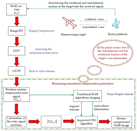
The block diagram of the proposed method is shown in Figure 3.
5. Simulation Analysis
We conduct three sets of experimental simulations to confirm the effectiveness of the proposed method. The simulation parameters of step frequency continuous wave (SFCW) radar are given in Table 1. Figure 4a,b show a hypothetical fighter target composed of perfect point scatterers and the amplitude of its raw data, respectively.
5.1. Imaging Results with Different Translational Motion Parameters
As can be seen from Figure 5, the RD algorithm causes the serious distortion of the imaging results, which is only used as a basic comparison algorithm here. Figure 5b shows that a good autofocus image can be obtained by using the GWT when the radial velocity of the target is small. As the radial velocity increases and the target has a larger acceleration, a serious range walk of the scatters occurs, negatively affecting the range resolution in Figure 6b and Figure 7b. As is obvious from Figure 7b, the uncompensated ISAR image is highly blurred due to the translational motion of the target, which proves that GWT cannot remove the severe translational motion effects from the ISAR image. Figure 5c, Figure 6c, and Figure 7c show the resultant motion-compensated ISAR image after applying the proposed method, and the image of the fighter is almost perfectly focused.
5.2. Imaging Results with Different Rotational Motion Parameters
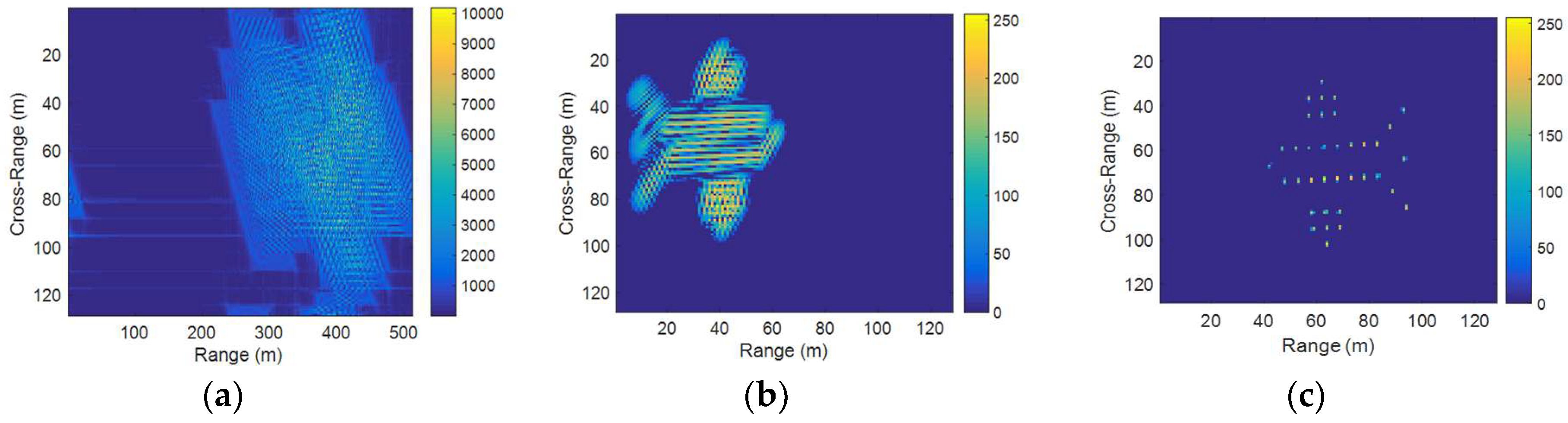
From the simulation results in Figure 8d, Figure 9c, and Figure 10c, we can see that the ISAR images of a non-uniform maneuvering target with a large angle and high speed can still be reconstructed by using the proposed method. This also indirectly verifies that GWT performs a good motion compensation for the maneuvering target that has an angular acceleration and large angular velocity, which is also a situation where the OSS phase retrieval is not suitable for application. Affected by the rotation component, the imaging result corresponding to OSS phase retrieval show that the parts of the point scatterers in Figure 8b are lost. Therefore, we no longer show the resultant images of phase retrieval under the condition that the target rotates at a larger angular velocity. The resultant raw range–Doppler ISAR image of the fighter by employing the GWT is depicted in Figure 8c, Figure 9b, and Figure 10b. As can be clearly seen from these figures, the effect of the target’s translational motion is severe in the resultant ISAR image, such that the image is blurred in the range and Doppler domains. Combining GWT with phase retrieval and after performing RMC and TMC, the resulting ISAR images after phase error correction become focused and clear.
5.3. The Spectrogram Comparison of Time Pulses in Each Part of the Proposed Method
To verify the feasibility of the proposed method, a further check is performed by observing the spectrogram of the received time pulses of the three different motion compensation stages with respect to Figure 7.
From these spectrograms, we can clearly observe the progressive shift in the frequency (or phase) of the received time pulses. The severe frequency shifts occur in Figure 11a, which appears as a nonlinearity of the frequency shift as a whole due to both the translational and the rotational motion of the target. As can be seen from Figure 11b, it clearly demonstrates that the frequency shifts of the time pulses are mitigated, in which the frequency shifts caused by the rotational motion have been removed by GWT, but there are still frequency shifts induced by the target translational velocity and acceleration. When all of the phase errors due to the translational and the rotational motion of the target are eliminated, all of the frequency (or the phase) values between the time pulses are well aligned, as shown in Figure 11c.
5.4. Imaging Results of Boeing 727 with Complex Motion
We also test the proposed method on the real data of a Boeing 727 airplane provided by the United States (U.S.) Naval Research Laboratory [21]. The parameters of the dataset are as follows: the carrier frequency is 9 GHz, the bandwidth is 150 MHz, and the pulse repetition frequency (PRF) is 25 KHz. The radar transmits 256 continuous bursts of stepped frequency waveform, each containing 128 pulses. Figure 12a,b show the ISAR image of Boeing 727 data with no motion and the amplitude spectrum of the data, respectively.
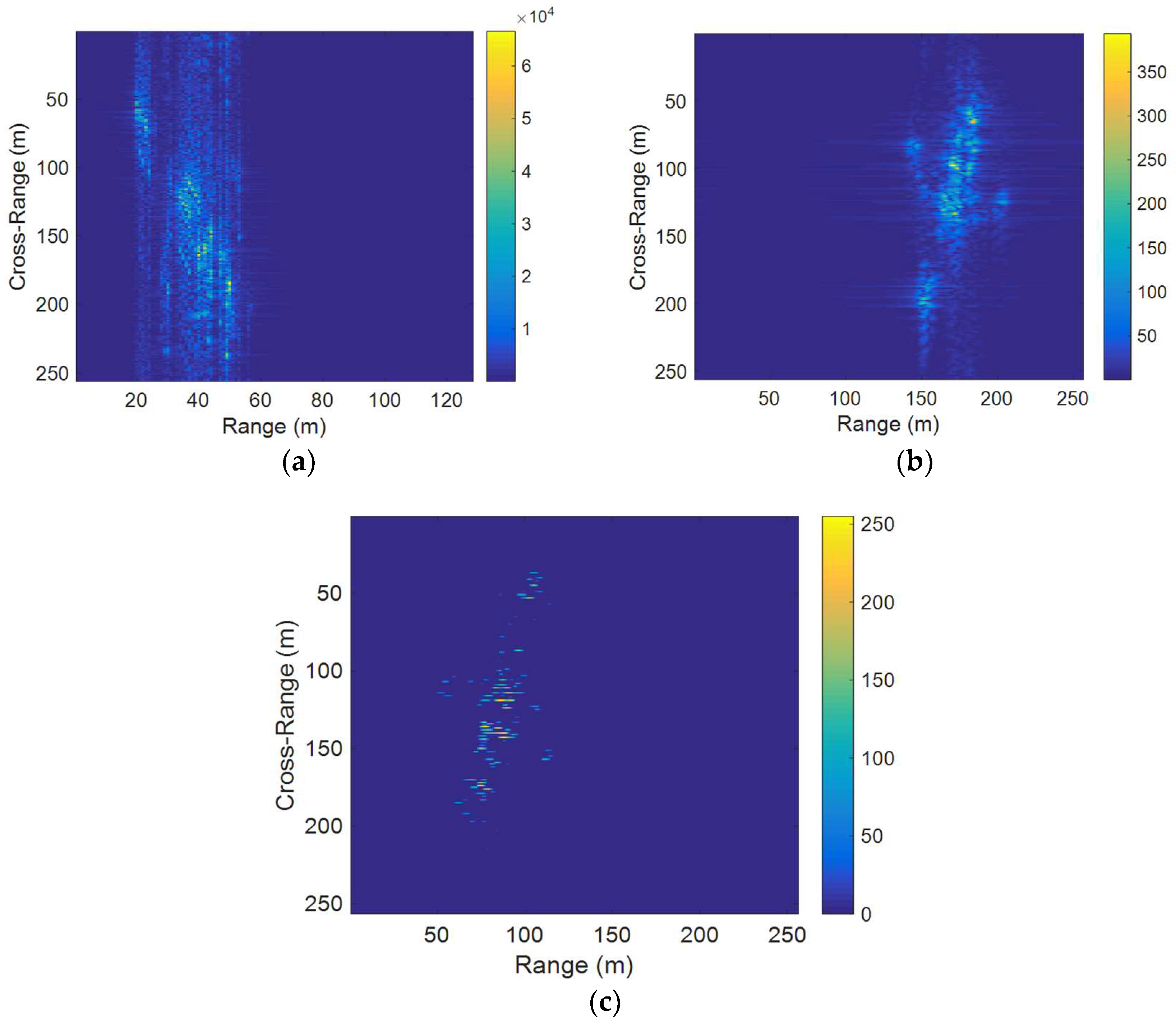
Similarly, because of the rotational motion and translational motion of the target, the ISAR image obtained through the range–Doppler algorithm is severely blurred, as shown in Figure 13a. To overcome the blurring, the Gabor wavelet transform is carried out first, and its imaging result is compared with that of the RD algorithm. As shown in Figure 13b, it clearly demonstrates that blurring is eliminated significantly in the image where only the translational motion-based defocusing is noted; that is, the errors associated with the target’s rotational motion are compensated by applying GWT. However, the residual translational component makes the defects obvious, so it must be removed through phase retrieval. The resultant image is given in Figure 13c, where all of the phase errors due to the translational and the rotational motion of the target were eliminated. The resultant motion-free ISAR image is very well focused, and the proposed method outperforms the RD and GWT algorithms in terms of the image quality.
6. Conclusions
A novel ISAR imaging method for maneuvering targets based on phase retrieval and Gabor wavelet transform has been proposed in this paper. RMC carried out by GWT is first applied to obtain an initial phase compensation. Furthermore, phase retrieval effectively overcomes the range walk issue of the scatters induced by the remaining translational component by aligning the range bins; that is, the scatterers remain in their range cells after applying the compensating procedure. After the RMC and TMC procedures, the time-invariant Doppler shifts can be obtained, and a clear and focused ISAR range–Doppler image can be formed. The process flow of the method is relatively simple, and there is no need to estimate the relevant motion parameters of the maneuvering target. Moreover, the results of this study confirm the feasibility of the method theory in this paper, and provide a new way of thinking for the maneuvering targets’ ISAR imaging problem.
Author Contributions
All the authors made significant contributions to this work. H.S. and T.Y. proposed the novel ISAR Imaging method; T.Y. performed the experiments and wrote the paper; Z.Q. revised the manuscript.
Funding
Shi’s work was supported by the National Natural Science Foundation of China (No. 61571388) and Natural Science Foundation of Hebei Province (No. F2016203251). Qiao’s work was partially supported by the President’s Endowed Professorship program of the University of Texas system. The APC was funded by the National Natural Science Foundation of China (No. 61571388).
Acknowledgments
The authors are very grateful to the Editor and reviewers for their constructive comments that have an important role in further improving this work.
Conflicts of Interest
The authors declare no conflict of interest.
References
- Wang, Y.; Kang, J.; Jiang, Y. ISAR Imaging of Maneuvering Target Based on the Local Polynomial Wigner Distribution and Integrated High-Order Ambiguity Function for Cubic Phase Signal Model. IEEE J. Sel. Top. Appl. Earth Observ. Remote Sens. 2017, 7, 2971–2991. [Google Scholar] [CrossRef]
- Zheng, J.; Su, T.; Liao, G.; Liu, H.; Liu, Z.; Liu, Q. ISAR Imaging for Fluctuating Ships Based on a Fast Bilinear Parameter Estimation Algorithm. IEEE J. Sel. Top. Appl. Earth Observ. Remote Sens. 2017, 8, 3954–3966. [Google Scholar] [CrossRef]
- An, P.; Ng, B.; Tran, H.T. Kurtosis-based estimation of cross-range scaling factor for high-resolution inverse synthetic aperture radar imaging. J. Appl. Remote Sens. 2016, 10, 030502. [Google Scholar] [CrossRef]
- Zeljković, V.; Li, Q.; Vincelette, R.; Tameze, C.; Liu, F. Automatic algorithm for inverse synthetic aperture radar images recognition and classification. IET Radar Sonar Navig. 2010, 4, 96–109. [Google Scholar] [CrossRef]
- Sadjadi, F.A. New experiments in inverse synthetic aperture radar image exploitation for maritime surveillance. Autom. Target Recognit. XXIV 2014, 9090, 909009. [Google Scholar] [CrossRef]
- Park, S.H. Automatic recognition of ISAR images of multiple targets and ATR results. Prog. Electromagn. Res. B 2014, 61, 43–54. [Google Scholar] [CrossRef]
- Zhou, Z.H.; Zhou, B.; Yeh, C.M. Methods for the rotation of ISAR images. Synthetic Aperture Radar. In Proceedings of the 2009 2nd Asian-Pacific Conference on Synthetic Aperture Radar, Xi’an, China, 26–30 October 2009; pp. 347–349. [Google Scholar] [CrossRef]
- Chen, C.C.; Andrews, H.C. Target-Motion Induced Radar Imaging. IEEE Trans. Aerosp. Electron. Syst. 1980, AES-16, 2–14. [Google Scholar] [CrossRef]
- Li, X.; Liu, G.; Ni, J. Autofocusing of ISAR images based on entropy minimization. IEEE Trans. Aerosp. Electron. Syst. 2002, 35, 1240–1252. [Google Scholar] [CrossRef]
- Wahl, D.E.; Eichel, P.H.; Ghiglia, D.C.; Jakowatz, C.V. Phase Gradient Autofocus—A Robust Tool for High Resolution SAR Phase Correction. IEEE Trans. Aerosp. Electron. Syst. 1994, 30, 827–835. [Google Scholar] [CrossRef]
- Xue, J.; Huang, L. An improved cross-correlation approach to parameter estimation based on fractional Fourier transform for ISAR motion compensation. In Proceedings of the 2015 IEEE International Conference on Acoustics, Speech and Signal Processing (ICASSP), Brisbane, Australia, 19–24 April 2015; pp. 1538–1542. [Google Scholar] [CrossRef]
- Pfeiffer, F.; Weitkamp, T.; Bunk, O.; David, C. Phase retrieval and differential phase-contrast imaging with low-brilliance X-ray sources. Nat. Phys. 2006, 2, 258–261. [Google Scholar] [CrossRef] [Green Version]
- Fogel, F.; Waldspurger, I.; D’Aspremont, A. Phase retrieval for imaging problems. Math. Program. Comput. 2016, 8, 311–335. [Google Scholar] [CrossRef] [Green Version]
- Luke, D.R.; Bauschke, H.H.; Combettes, P.L. Phase retrieval, error reduction algorithm, and Fienup variants: A view from convex optimization. J. Opt. Soc. Am. A Opt. Image Sci. Vis. 2002, 19, 1334–1345. [Google Scholar] [CrossRef]
- Rodriguez, J.A.; Xu, R.; Chen, C.C.; Zou, Y.; Miao, J. Oversampling smoothness: An effective algorithm for phase retrieval of noisy diffraction intensities. J. Appl. Crystallogr. 2013, 46, 312. [Google Scholar] [CrossRef] [PubMed]
- Shi, H.; Xia, S. ISAR imaging based on oversampling smoothness of prior knowledge. In Proceedings of the 2016 IEEE 13th International Conference on Signal Processing (ICSP), Chengdu, China, 6–10 November 2016; pp. 1597–1600. [Google Scholar] [CrossRef]
- Shi, H.; Xia, S.; Tian, Y. ISAR imaging based on improved phase retrieval algorithm. J. Syst. Eng. Electron. 2018, 29, 278–285. [Google Scholar] [CrossRef]
- Netrapalli, P.; Jain, P.; Sanghavi, S. Phase retrieval using alternating minimization. IEEE Trans. Signal Process. 2015, 63, 4814–4826. [Google Scholar] [CrossRef]
- Chen, V.C.; Qian, S. Joint time-frequency transform for radar range-Doppler imaging. IEEE Trans. Aerosp. Electron. Syst. 1998, 34, 486–499. [Google Scholar] [CrossRef]
- Mallat, S.G.; Zhang, Z. Matching pursuits with time-frequency dictionaries. IEEE Trans. Signal Process. 1993, 41, 3397–3415. [Google Scholar] [CrossRef] [Green Version]
- Wang, Y.; Ling, H.; Chen, C.C. ISAR motion compensation via adaptive joint time-frequency technique. IEEE Trans. Aerosp. Electron. Syst. 1998, 34, 670–677. [Google Scholar] [CrossRef]
- Wang, Z.; Yang, W.; Chen, Z.; Zhao, Z.; Hu, H.; Qi, C. A Novel Adaptive Joint Time Frequency Algorithm by the Neural Network for the ISAR Rotational Compensation. Remote Sens. 2018, 10, 334. [Google Scholar] [CrossRef]
- Berizzi, F.; Corsini, G. Autofocusing of Inverse Synthetic Aperture Radar Images Using Contrast Optimization. IEEE Trans. Aerosp. Electron. Syst. 1996, 32, 1185–1191. [Google Scholar] [CrossRef]
- Hu, C.; Ferrofamil, L.; Kuang, G. Ship discrimination using polarimetric SAR data and coherent time-frequency analysis. Remote Sens. 2013, 5, 6899–6920. [Google Scholar] [CrossRef] [Green Version]
- Qian, S.; Chen, D. Decomposition of the Wigner-Ville distribution and time-frequency distribution series. IEEE Trans. Signal Process 1994, 42, 2836–2842. [Google Scholar] [CrossRef]
- Thomas, G.; Flores, B.C.; Martinez, A. ISAR imaging of moving targets via the Gabor wavelet transform. Proc. SPIE–Int. Soc. Opt. Eng. 1997, 3161. [Google Scholar] [CrossRef]
- Wang, F.; Sheng, W.X.; Ma, X.F.; Wang, H. ISAR Image Recognition with Fusion of Gabor Magnitude and Phase Feature. J. Electron. Inf. Technol. 2013, 35, 1813–1819. [Google Scholar] [CrossRef]
- Park, J.H.; Myung, N.H. Enhanced and Efficient ISAR Image Focusing Using the Discrete Gabor Representation in an Oversampling Scheme. Prog. Electomang. Res. 2013, 138, 227–244. [Google Scholar] [CrossRef]
- Chen, V.C.; Martorella, M. Inverse Synthetic Aperture Radar Imaging: Principles, Algorithms and Applications; SciTech Publishing: Edison, NJ, USA, 2014; pp. 70–71. [Google Scholar]
- Fienup, J.R. Phase retrieval algorithms: A comparison. Appl. Opt. 1982, 21, 2758–2769. [Google Scholar] [CrossRef] [PubMed]
Figure 1.
Geometry for a maneuvering target with respect to radar.
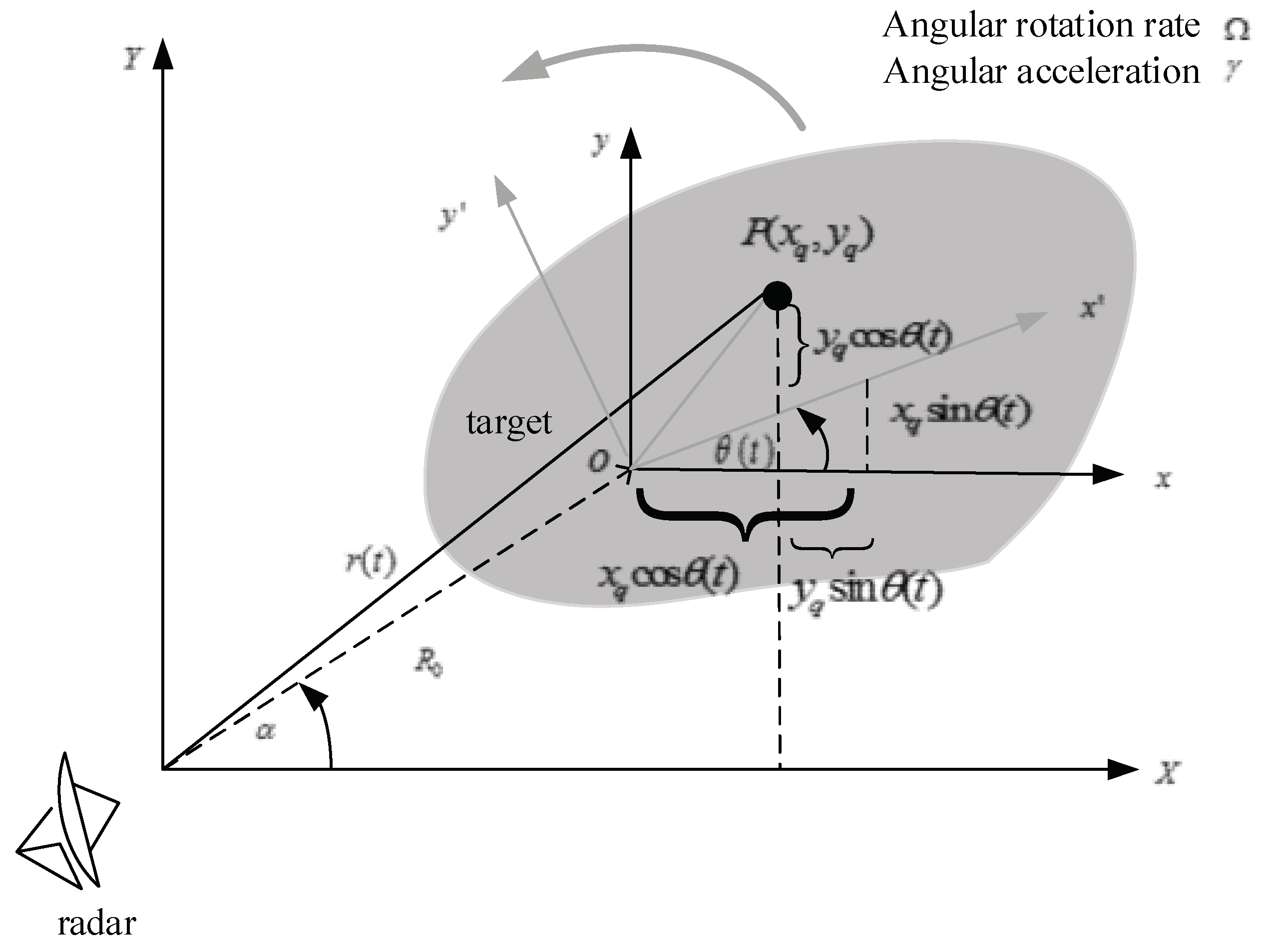
Figure 2.
Overall procedures of the Gabor wavelet transform (GWT)-based inverse synthetic aperture radar (ISAR) imaging.
Figure 2.
Overall procedures of the Gabor wavelet transform (GWT)-based inverse synthetic aperture radar (ISAR) imaging.

Figure 3.
Block diagram of the proposed method.

Figure 4.
(a) A fighter target composed of perfect point scatterers; (b) The amplitude of the raw data.
Figure 4.
(a) A fighter target composed of perfect point scatterers; (b) The amplitude of the raw data.
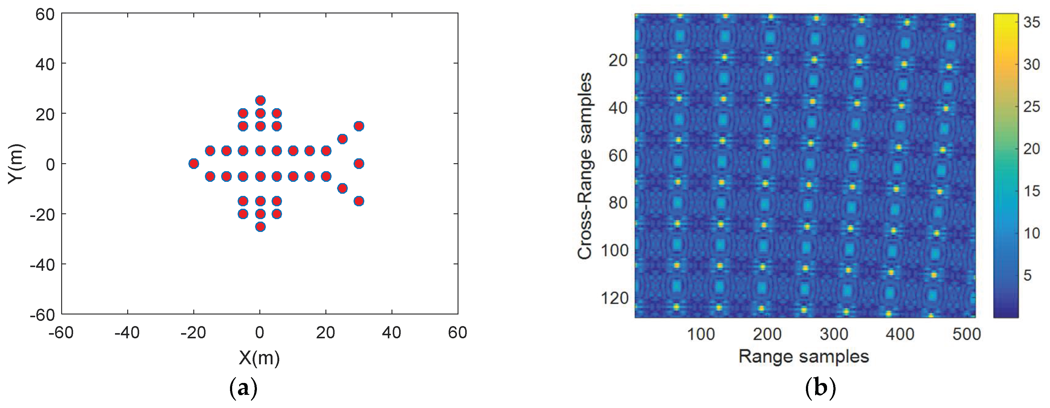
Figure 5.
Target’s simulation motion parameters are . (a) Range–Doppler (RD) algorithm; (b) GWT; (c) the proposed method.
Figure 5.
Target’s simulation motion parameters are . (a) Range–Doppler (RD) algorithm; (b) GWT; (c) the proposed method.

Figure 6.
Target’s simulation motion parameters are . (a) RD algorithm; (b) GWT; (c) the proposed method.
Figure 6.
Target’s simulation motion parameters are . (a) RD algorithm; (b) GWT; (c) the proposed method.
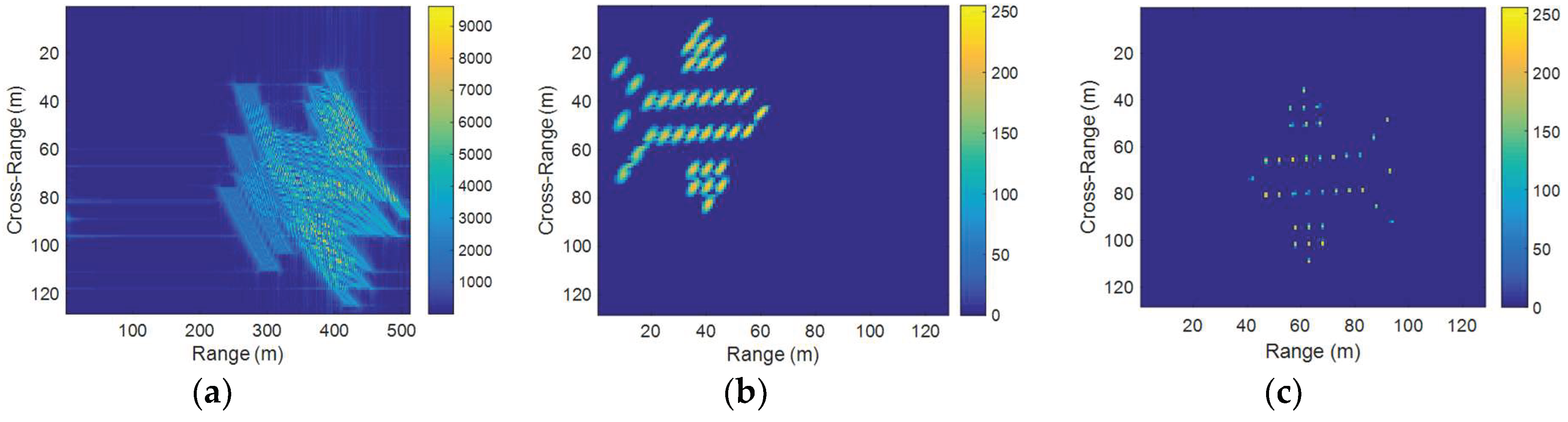
Figure 7.
Target’s simulation motion parameters are . (a) RD algorithm; (b) GWT; (c) the proposed method.
Figure 7.
Target’s simulation motion parameters are . (a) RD algorithm; (b) GWT; (c) the proposed method.

Figure 8.
Target’s simulation motion parameters are . (a) RD algorithm; (b) oversampling smoothness (OSS) phase retrieval; (c) GWT; (d) the proposed method.
Figure 8.
Target’s simulation motion parameters are . (a) RD algorithm; (b) oversampling smoothness (OSS) phase retrieval; (c) GWT; (d) the proposed method.
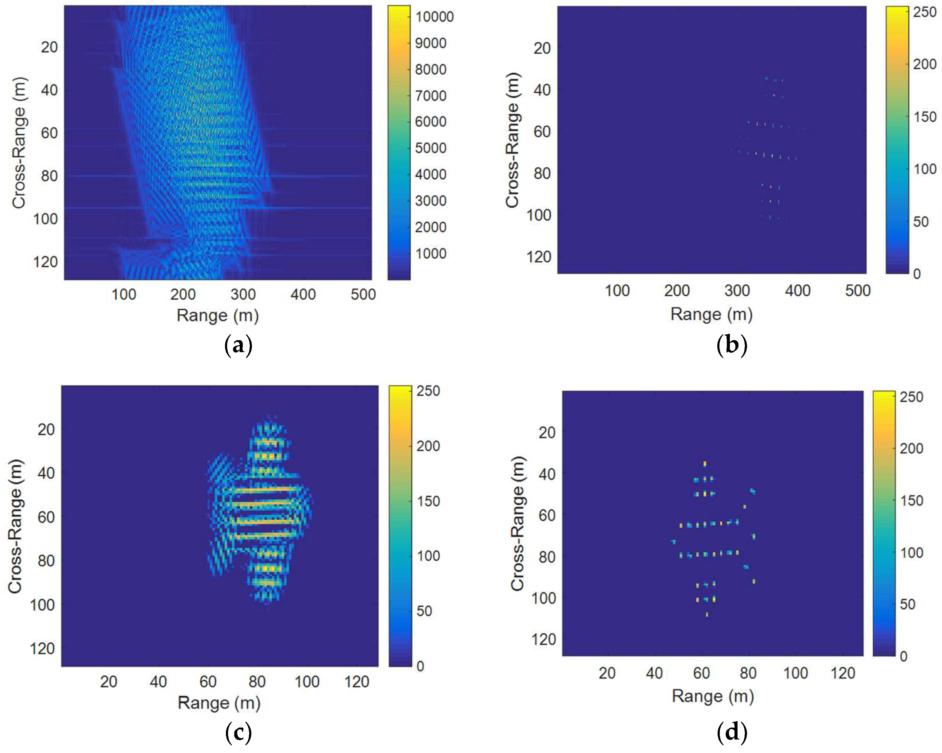
Figure 9.
Target’s simulation motion parameters are . (a) RD algorithm; (b) GWT; (c) the proposed method.
Figure 9.
Target’s simulation motion parameters are . (a) RD algorithm; (b) GWT; (c) the proposed method.

Figure 10.
Target’s simulation motion parameters are . (a) RD algorithm; (b) GWT; (c) the proposed method.
Figure 10.
Target’s simulation motion parameters are . (a) RD algorithm; (b) GWT; (c) the proposed method.

Figure 11.
Spectrograms of time pulses with the different part of the proposed method. (a) no compensation (RD); (b) after rotational motion compensation (GWT); (c) after translational and rotational motion compensation (the proposed method).
Figure 11.
Spectrograms of time pulses with the different part of the proposed method. (a) no compensation (RD); (b) after rotational motion compensation (GWT); (c) after translational and rotational motion compensation (the proposed method).
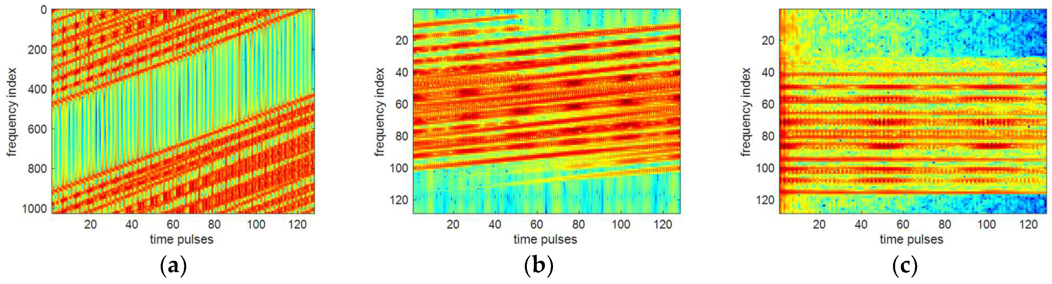
Figure 12.
Data of Boeing 727. (a) ISAR image with no motion; (b) The amplitude of the data.

Figure 13.
Imaging results of real data with complex motion. (a) RD algorithm; (b) GWT; (c) the proposed method.
Figure 13.
Imaging results of real data with complex motion. (a) RD algorithm; (b) GWT; (c) the proposed method.

Table 1.
The radar parameters for step frequency continuous wave (SFCW) illumination.
| Parameter Name | Symbol | Value |
|---|---|---|
| The initial range of the target | R0 | 10 km |
| Carrier frequency | fc | 3 GHz |
| Frequency bandwidth | B | 217 MHz |
| Pulse repetition frequency | PRF | 40 KHz |
| Number of pulses | N | 128 |
| Number of bursts | M | 512 |
© 2018 by the authors. Licensee MDPI, Basel, Switzerland. This article is an open access article distributed under the terms and conditions of the Creative Commons Attribution (CC BY) license (http://creativecommons.org/licenses/by/4.0/).
Share and Cite
MDPI and ACS Style
Shi, H.; Yang, T.; Qiao, Z. ISAR Autofocus Imaging Algorithm for Maneuvering Targets Based on Phase Retrieval and Gabor Wavelet Transform. Remote Sens. 2018, 10, 1810. https://doi.org/10.3390/rs10111810
AMA Style
Shi H, Yang T, Qiao Z. ISAR Autofocus Imaging Algorithm for Maneuvering Targets Based on Phase Retrieval and Gabor Wavelet Transform. Remote Sensing. 2018; 10(11):1810. https://doi.org/10.3390/rs10111810
Chicago/Turabian StyleShi, Hongyin, Ting Yang, and Zhijun Qiao. 2018. "ISAR Autofocus Imaging Algorithm for Maneuvering Targets Based on Phase Retrieval and Gabor Wavelet Transform" Remote Sensing 10, no. 11: 1810. https://doi.org/10.3390/rs10111810
Note that from the first issue of 2016, this journal uses article numbers instead of page numbers. See further details here.