Mass Balance of Novaya Zemlya Archipelago, Russian High Arctic, Using Time-Variable Gravity from GRACE and Altimetry Data from ICESat and CryoSat-2


Abstract

1. Introduction
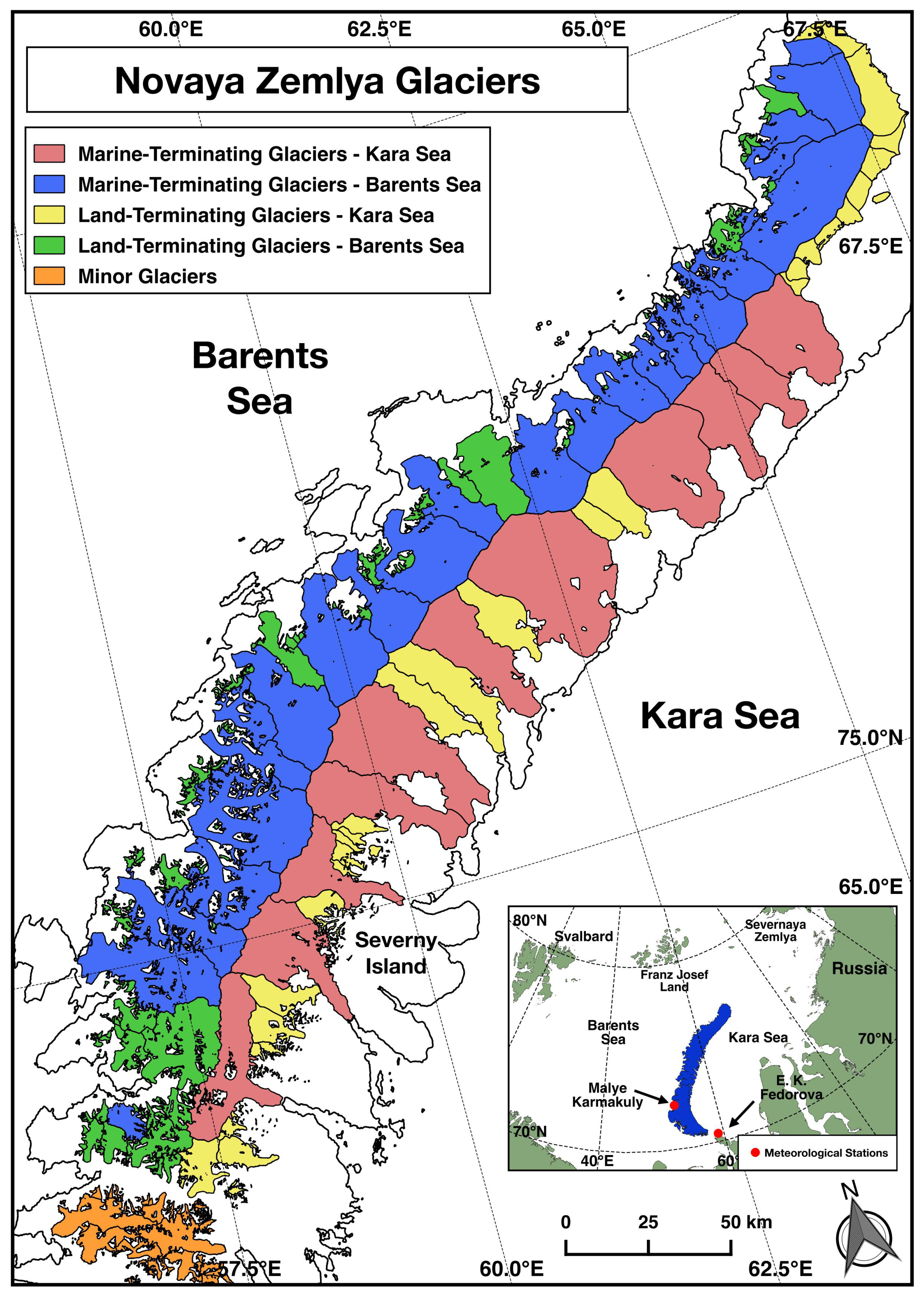
2. Study Region
Prior Studies
3. Data and Methods
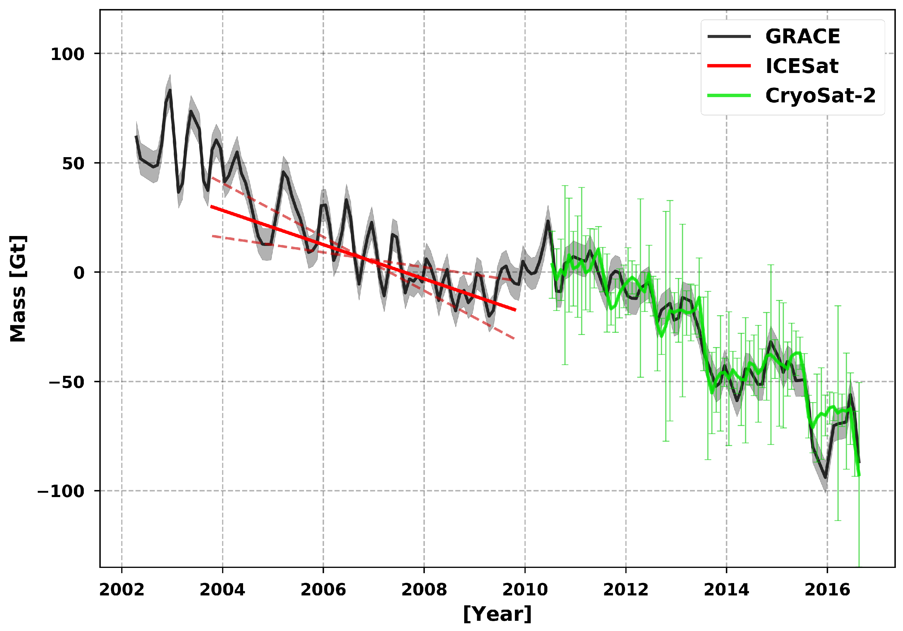
3.1. Time-Variable Gravity
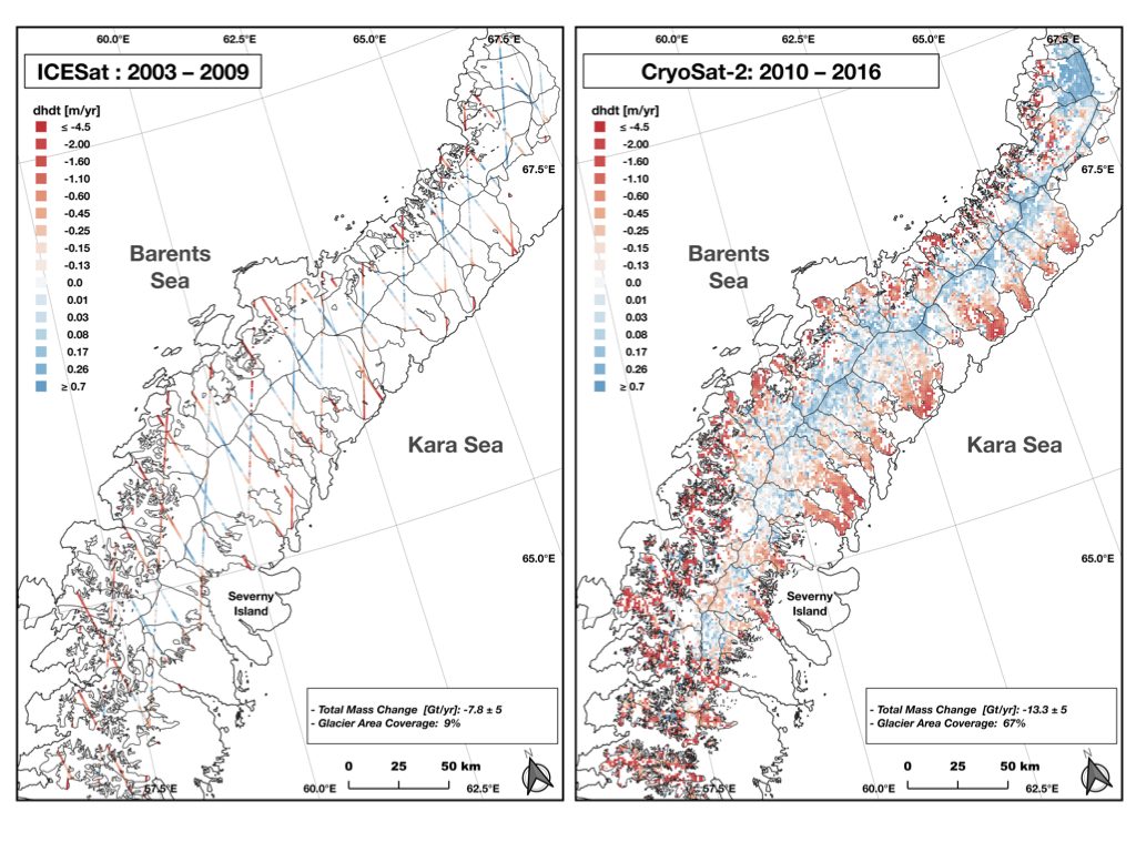
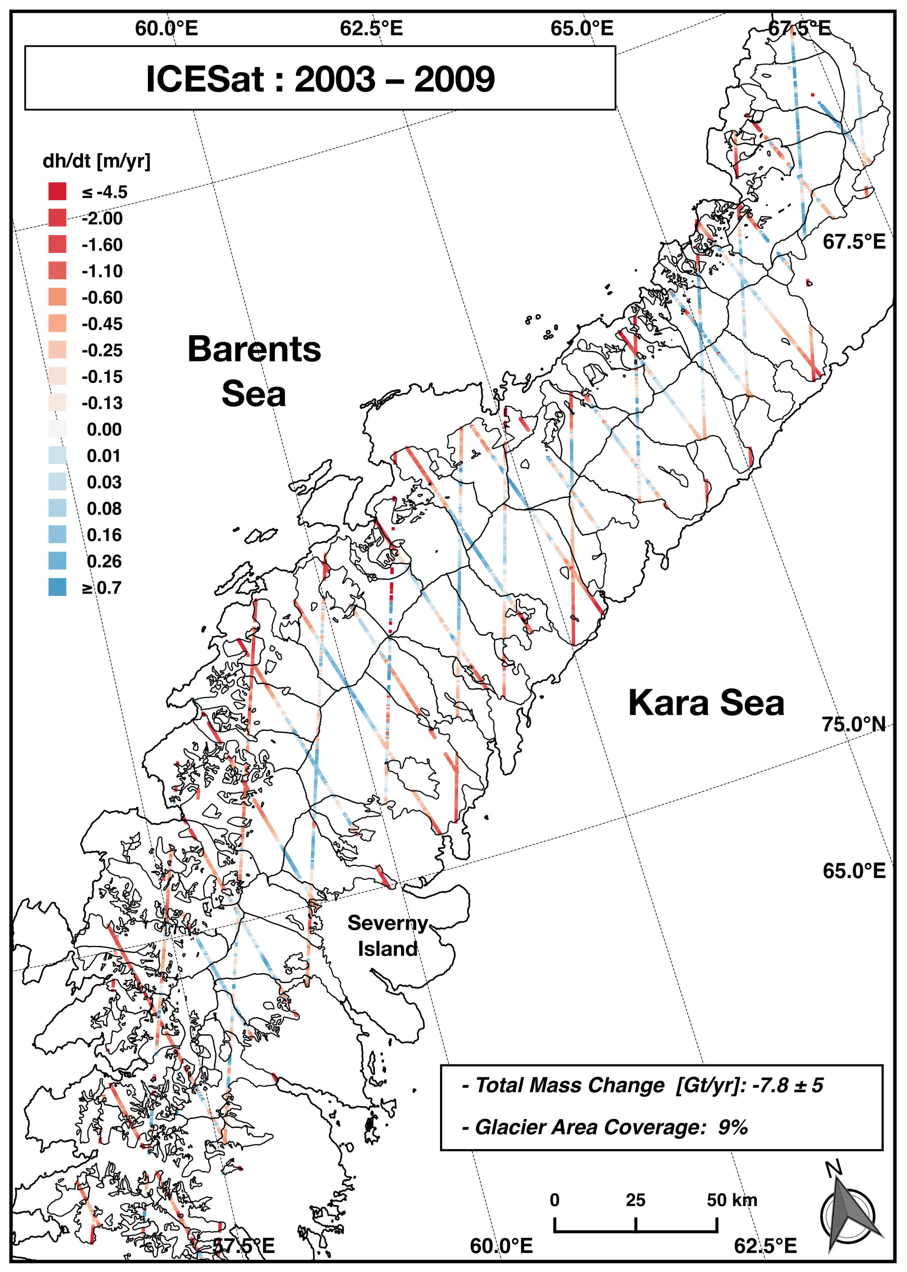
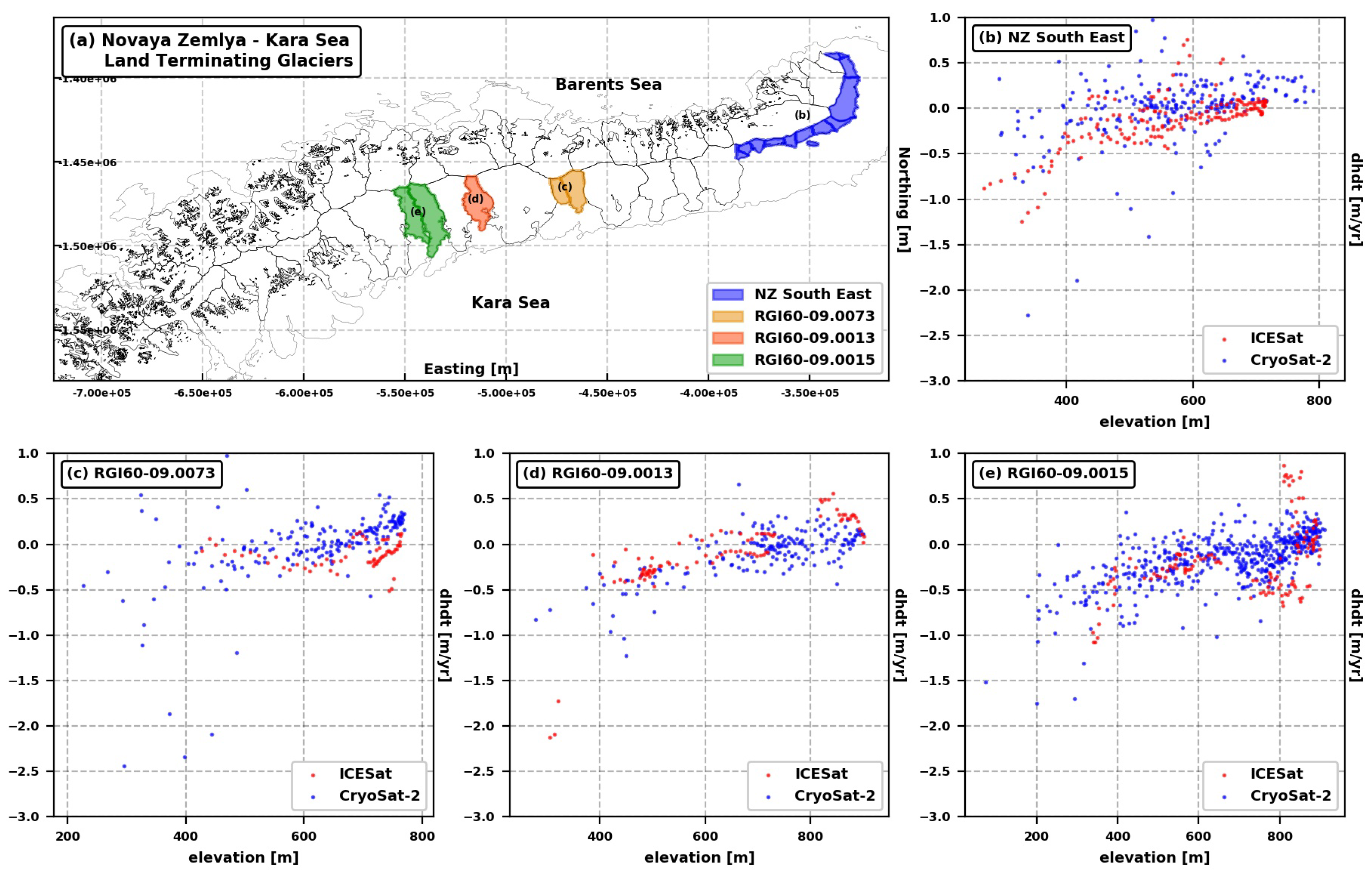
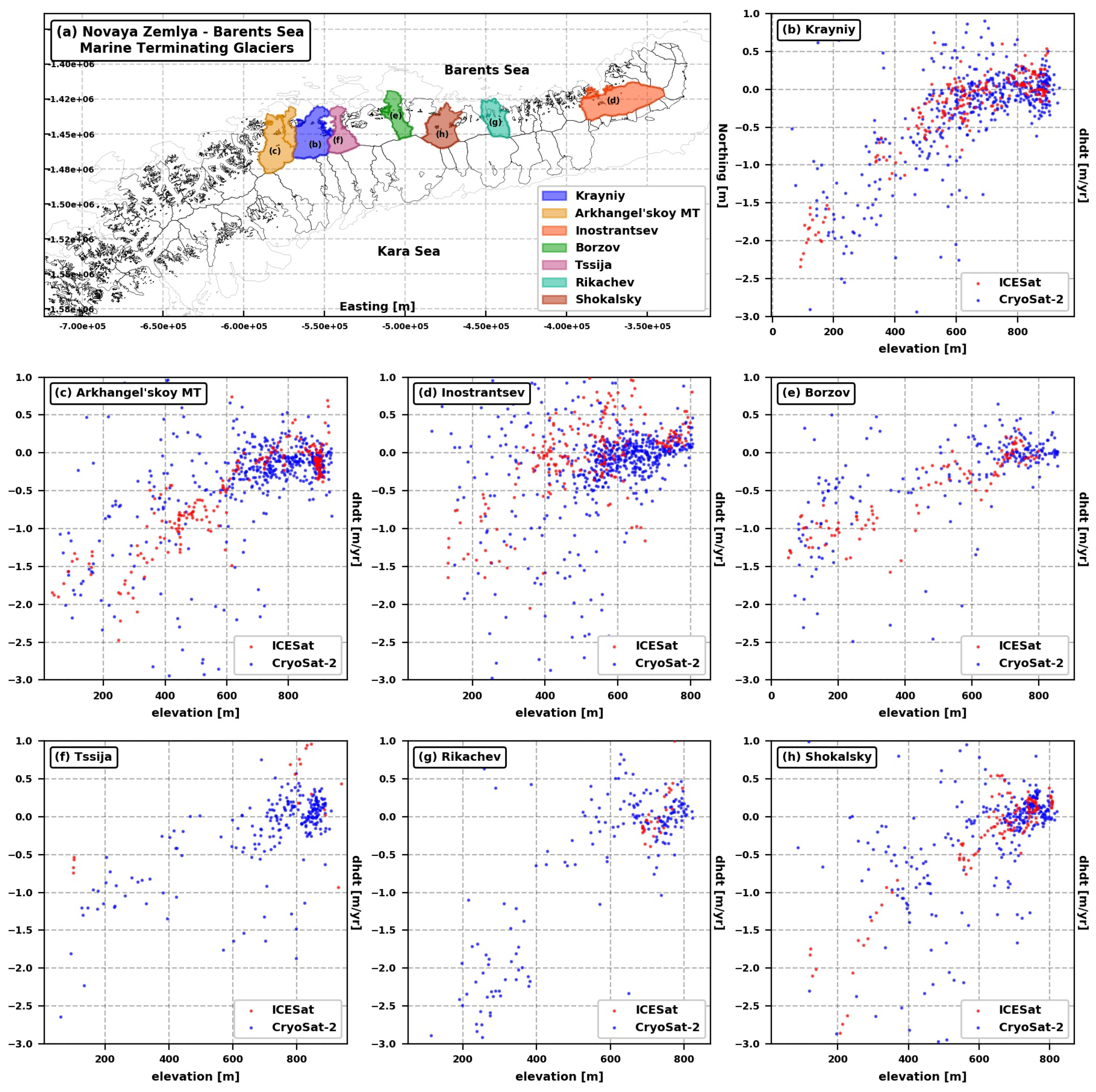
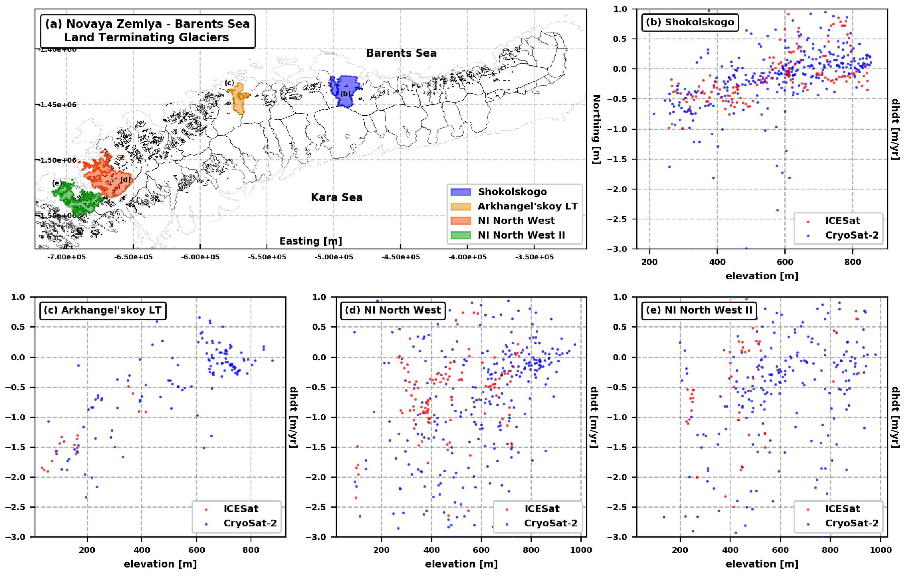
3.2. ICESat Altimetry
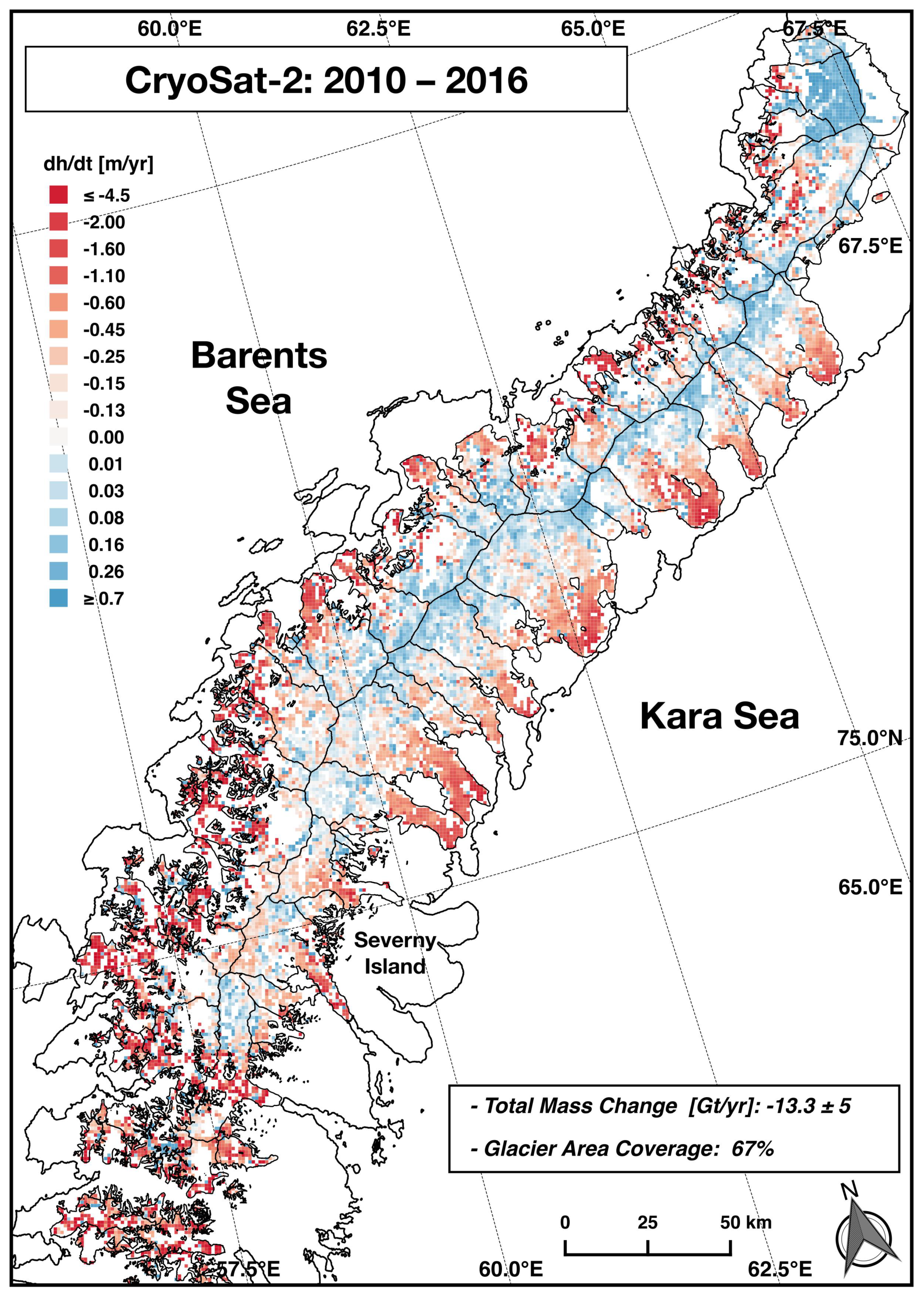
3.3. CryoSat-2
Averaging Procedure
- If the considered grid cell contains a single measurement, we assign this value to the entire grid cell;
- If the considered grid cell contains multiple measurements, we set its elevation change rate equal to the measurements mean. We use a 3- iterative filter in order to discard erroneous observations that could influence our final elevation change estimate.
3.4. Spatial Extrapolation
- We find all the measurements available within a distance smaller than or equal to a selected search radius and we evaluate the quadratic polynomial function that provides the best parametrization of the relation between the considered elevation change estimates and their mean elevation.
- We assign the considered grid cell an elevation change value calculated using the parameters from the quadratic polynomial fit and the average elevation of the grid cell provided by ArcticDEM.
3.5. From Volume to Mass Change
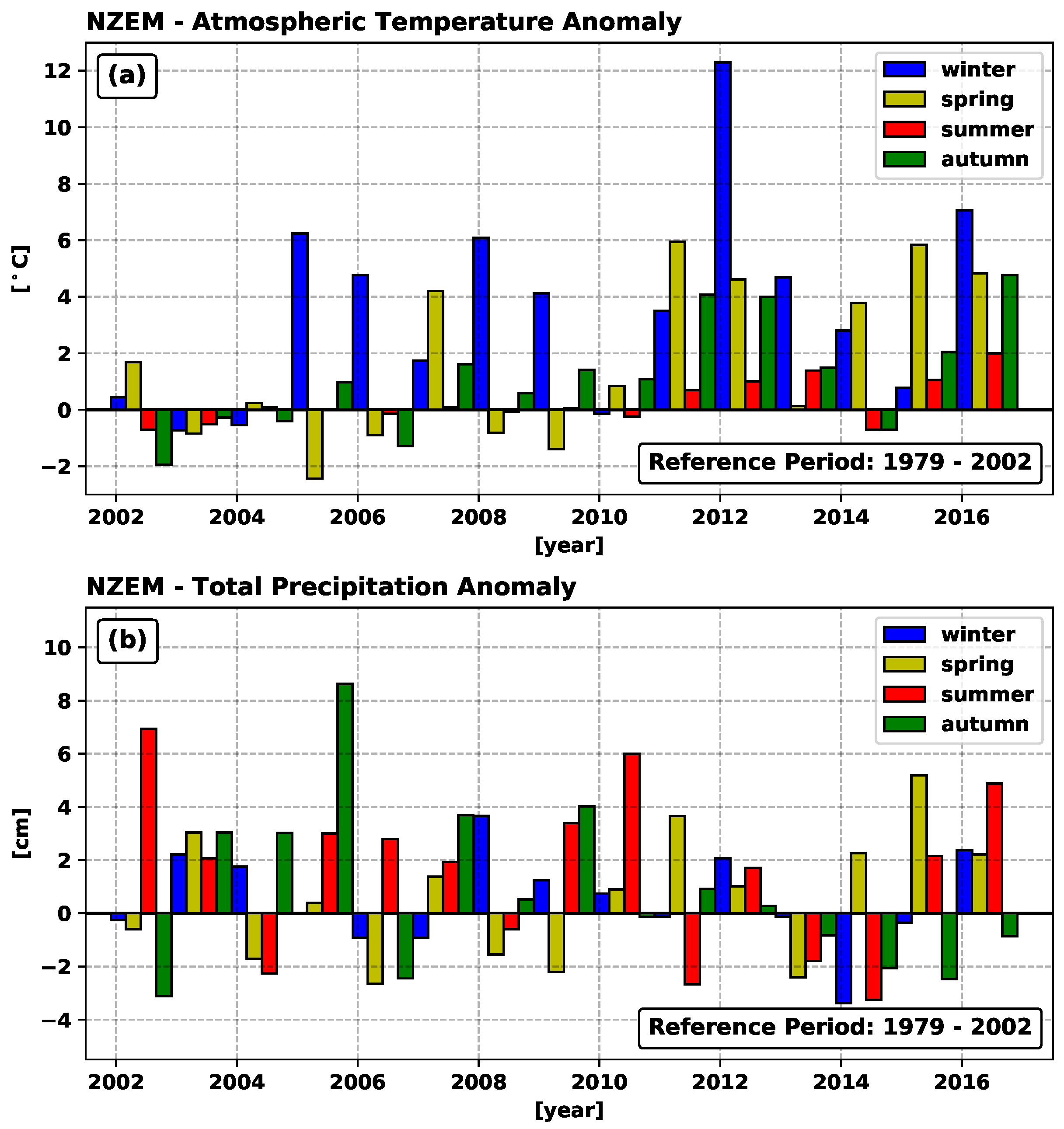
3.6. Atmospheric Temperatures and Total Precipitation
4. Results
5. Discussion
6. Conclusions
Author Contributions
Funding
Acknowledgments
Conflicts of Interest
Abbreviations
| GIC | Glaciers And Ice Caps |
| RHA | Russian High Arctic |
| NZEM | Novaya Zemlya Archipelago |
| SLR | Sea-Level Rise |
| SMB | Surface Mass Balance |
| D | Discharge |
| NAO | North Atlantic Oscillation |
| AW | Atlantic Water |
| DLR | German Aerospace Center |
| RL05 | GRACE Fifth Data Release |
| RL04 | GRACE Fourth Data Release |
| CSR | Center for Space Research at 133 the University of Texas |
| SLR | Satellite Laser Ranging |
| GIA | Glacial Isostatic Adjustment |
| LGM | Last Glacial Maximum |
| SIRAL | SAR/Interferometric Radar Altimeter (SIRAL) |
| SARIn | SAR interferometry mode |
| POCA | Point of Closest Approach |
Appendix A. Glacier Inventories
Appendix B. Time Series of Ice Elevation Change
Appendix C. Spatial Extrapolation—Local Regression Filter
Appendix D. Uncertainty Analysis
- Elevation change measurement error ();
- Extrapolation error ();
- Error in glacier area ();
- Sampling Bias Error (due to the non-uniform distribution of the elevation change measurements on the glacier surface) ();
- Error associated with the volume to mass conversion ();
References
- Zuo, Z.; Oerlemans, J. Contribution of glacier melt to sea-level rise since AD 1865: A regionally differentiated calculation. Clim. Dyn. 1997, 13, 835–845. [Google Scholar] [CrossRef]
- Marzeion, B.; Champollion, N.; Haeberli, W.; Langley, K.; Leclercq, P.; Paul, F. Observation-Based Estimates of Global Glacier Mass Change and Its Contribution to Sea-Level Change. Surv. Geophys. 2017, 38, 105–130. [Google Scholar] [CrossRef] [PubMed]
- Dowdeswell, J.A.; Hagen, J.O.; Björnsson, H.; Glazovsky, A.F.; Harrison, W.D.; Holmlund, P.; Jania, J.; Koerner, R.M.; Lefauconnier, B.; Ommanney, C.L.; et al. The Mass Balance of Circum-Arctic Glaciers and Recent Climate Change. Quat. Res. 1997, 48, 1–14. [Google Scholar] [CrossRef]
- Meier, M.F.; Dyurgerov, M.B.; Rick, U.K.; O’Neel, S.; Pfeffer, W.T.; Anderson, R.S.; Anderson, S.P.; Glazovsky, A.F. Glaciers Dominate Eustatic Sea-Level Rise in the 21st Century. Science 2007, 317, 1064–1067. [Google Scholar] [CrossRef] [PubMed]
- Vaughan, D.; Comiso, J.; Allison, I.; Carrasco, J.; Kaser, G.; Kwok, R.; Mote, P.; Murray, T.; Paul, F.; Ren, J.; et al. Observations: Cryosphere. In Climate Change 2013: The Physical Science Basis. Contribution of Working Group I to the Fifth Assessment Report of the Intergovernmental Panel on Climate Change; Cambridge University Press: Cambridge, UK, 2013; pp. 317–382. [Google Scholar]
- Reager, J.T.; Gardner, A.S.; Famiglietti, J.S.; Wiese, D.N.; Eicker, A.; Lo, M.H. A decade of sea level rise slowed by climate-driven hydrology. Science 2016, 351, 699–703. [Google Scholar] [CrossRef] [PubMed]
- Ciracì, E.; Velicogna, I.; Swenson, S. Acceleration in mass loss of the world glaciers and ice caps using time-variable gravity data from the 2002-2017 GRACE mission. Earth Planet. Sci. Lett. 2018. Unpublished work. [Google Scholar]
- Screen, J.A.; Simmonds, I. The central role of diminishing sea ice in recent Arctic temperature amplification. Nature 2010, 464, 1334. [Google Scholar] [CrossRef] [PubMed]
- Serreze, M.C.; Barrett, A.P.; Slater, A.G.; Woodgate, R.A.; Aagaard, K.; Lammers, R.B.; Steele, M.; Moritz, R.; Meredith, M.; Lee, C.M. The large-scale freshwater cycle of the Arctic. J. Geophys. Res. Oceans 2006, 111. [Google Scholar] [CrossRef]
- Cohen, J.; Screen, J.A.; Furtado, J.C.; Barlow, M.; Whittleston, D.; Coumou, D.; Francis, J.; Dethloff, K.; Entekhabi, D.; Overland, J.; Jones, J. Recent Arctic amplification and extreme mid-latitude weather. Nat. Geosci. 2014, 7. [Google Scholar] [CrossRef]
- Moholdt, G.; Wouters, B.; Gardner, A.S. Recent mass changes of glaciers in the Russian High Arctic. Geophys. Res. Lett. 2012, 39, L10502. [Google Scholar] [CrossRef]
- Jacob, T.; Wahr, J.; Pfeffer, W.T.; Swenson, S. Recent contributions of glaciers and ice caps to sea level rise. Nature 2012, 482, 514–518. [Google Scholar] [CrossRef] [PubMed]
- Melkonian, A.K.; Willis, M.J.; Pritchard, M.E.; Stewart, A.J. Recent changes in glacier velocities and thinning at Novaya Zemlya. Remote Sens. Environ. 2016, 174, 244–257. [Google Scholar] [CrossRef]
- Carr, J.R.; Bell, H.; Killick, R.; Holt, T. Exceptional retreat of Novaya Zemlya’s marine-terminating outlet glaciersbetween 2000 and 2013. Cryosphere 2017, 11, 2149–2174. [Google Scholar] [CrossRef]
- Strozzi, T.; Paul, F.; Wiesmann, A.; Schellenberger, T.; Kääb, A. Circum-Arctic Changes in the Flow of Glaciers and Ice Caps from Satellite SAR Data between the 1990s and 2017. Remote Sens. 2017, 9, 947. [Google Scholar] [CrossRef]
- Gardner, A.S.; Moholdt, G.; Wouters, B.; Wolken, G.J.; Burgess, D.O.; Sharp, M.J.; Cogley, J.G.; Braun, C.; Labine, C. Sharply increased mass loss from glaciers and ice caps in the Canadian Arctic Archipelago. Nature 2011, 473, 357–360. [Google Scholar] [CrossRef] [PubMed]
- Lenaerts, J.T.M.; van Angelen, J.H.; van den Broeke, M.R.; Gardner, A.S.; Wouters, B.; van Meijgaard, E. Irreversible mass loss of Canadian Arctic Archipelago glaciers. Geophys. Res. Lett. 2013, 40, 870–874. [Google Scholar] [CrossRef]
- Van Wychen, W.; Burgess, D.O.; Gray, L.; Copland, L.; Sharp, M.; Dowdeswell, J.A.; Benham, T.J. Glacier velocities and dynamic ice discharge from the Queen Elizabeth Islands, Nunavut, Canada. Geophys. Res. Lett. 2014, 41, 2013GL058558. [Google Scholar] [CrossRef]
- Millan, R.; Mouginot, J.; Rignot, E. Mass budget of the glaciers and ice caps of the Queen Elizabeth Islands, Canada, from 1991 to 2015. Environ. Res. Lett. 2017, 12, 024016. [Google Scholar] [CrossRef]
- Larsen, C.F.; Burgess, E.; Arendt, A.A.; O’Neel, S.; Johnson, A.J.; Kienholz, C. Surface melt dominates Alaska glacier mass balance. Geophys. Res. Lett. 2015, 42, 2015GL064349. [Google Scholar] [CrossRef]
- Radić, V.; Bliss, A.; Beedlow, A.C.; Hock, R.; Miles, E.; Cogley, J.G. Regional and global projections of twenty-first century glacier mass changes in response to climate scenarios from global climate models. Clim. Dyn. 2014, 42, 37–58. [Google Scholar] [CrossRef]
- Kotlyakov, V.M.; Glazovskii, A.F.; Frolov, I.E. Glaciation in the arctic. Her. Russ. Acad. Sci. 2010, 80, 155–164. [Google Scholar] [CrossRef]
- Arendt, A.A.; Bliss, A.; Bolch, T.; Cogley, J.G.; Gardner, A.S.; Hagen, J.O.; Hock, R.; Kaser, G.; Kienholz, C.; Miles, E.; et al. The Randolph Glacier Inventory: A globally complete inventory of glaciers. J. Glaciol. 2014, 60, 537–552. [Google Scholar] [CrossRef]
- Rastner, P.; Strozzi, T.; Paul, F. Fusion of Multi-Source Satellite Data and DEMs to Create a New Glacier Inventory for Novaya Zemlya. Remote Sens. 2017, 9, 1122. [Google Scholar] [CrossRef]
- Grosval’d, M.G.; Kotlyakov, V.M. Present-Day Glaciers in the U.S.S.R. and Some Data on their Mass Balance. J. Glaciol. 1969, 8. [Google Scholar] [CrossRef]
- Zeeberg, J.J.; Forman, S.L.; Polyak, L. Glacier extent in a Novaya Zemlya fjord during the “Little Ice Age” inferred from glaciomarine sediment records. Polar Res. 2003, 22, 385–394. [Google Scholar] [CrossRef]
- Grant, K.L.; Stokes, C.R.; Evans, I.S. Identification and characteristics of surge-type glaciers on Novaya Zemlya, Russian Arctic. J. Glaciol. 2009, 55, 960–972. [Google Scholar] [CrossRef]
- Zeeberg, J. Climate and Glacial History of the Novaya Zemlya Archipelago, Russian Arctic; Rozenberg Publishers: Amsterdam, The Netherlands, 2001; ISBN 9051705638. [Google Scholar]
- Venegas, S.A.; Mysak, L.A. Is There a Dominant Timescale of Natural Climate Variability in the Arctic? J. Clim. 2000, 13, 3412–3434. [Google Scholar] [CrossRef]
- Dickson, R.R.; Osborn, T.J.; Hurrell, J.W.; Meincke, J.; Blindheim, J.; Adlandsvik, B.; Vinje, T.; Alekseev, G.; Maslowski, W. The Arctic Ocean Response to the North Atlantic Oscillation. J. Clim. 2000, 13, 2671–2696. [Google Scholar] [CrossRef]
- Przybylak, R.; Wyszyński, P. Air temperature in Novaya Zemlya Archipelago and Vaygach Island from 1832 to 1920 in the light of early instrumental data. Int. J. Climatol. 2016, 37, 3491–3508. [Google Scholar] [CrossRef]
- Zeeberg, J.; Forman, S.L. Changes in glacier extent on north Novaya Zemlya in the twentieth century. Holocene 2001, 11, 161–175. [Google Scholar] [CrossRef]
- Williams, R.; Ferrigno, J. Glaciers of Asia: U.S. Geological Survey. Prof. Pape 2010, 1386-F, 349. [Google Scholar]
- Sharov, A.; Schöner, W.; Pail, R. Spatial Features of Glacier Changes in the Barents-Kara Sector. In Proceedings of the EGU General Assembly Conference, Vienna, Austria, 19–24 April 2009; Volume 11, p. 3046. [Google Scholar] [CrossRef]
- Hurrell, J.W. Influence of variations in extratropical wintertime teleconnections on northern hemisphere temperature. Geophys. Res. Lett. 1996, 23, 665–668. [Google Scholar] [CrossRef]
- Pelto, M. Recent Climate Change Impacts on Mountain Glaciers; Wiley-Blackwell: Hoboken, NJ, USA, 2016; Chapter 11; pp. 171–186. [Google Scholar]
- Zhao, M.; Ramage, J.; Semmens, K.; Obleitner, F. Recent ice cap snowmelt in Russian High Arctic and anti-correlation with late summer sea ice extent. Environ. Res. Lett. 2014, 9, 045009. [Google Scholar] [CrossRef]
- Carr, R.; R Stokes, C.; Vieli, A. Recent retreat of major outlet glaciers on Novaya Zemlya, Russian Arctic, influenced by fjord geometry and sea-ice conditions. J. Glaciol. 2014, 60, 155–170. [Google Scholar] [CrossRef]
- Sun, Z.; Lee, H.; Ahn, Y.; Aierken, A.; Tseng, K.H.; Okeowo, M.A.; Shum, C.K. Recent Glacier Dynamics in the Northern Novaya Zemlya Observed by Multiple Geodetic Techniques. IEEE J. Sel. Top. Appl. Earth Observ. Remote Sens. 2017, 10, 1290–1302. [Google Scholar] [CrossRef]
- Tapley, B.D.; Bettadpur, S.; Watkins, M.; Reigber, C. The gravity recovery and climate experiment: Mission overview and early results. Geophys. Res. Lett. 2004, 31, L09607. [Google Scholar] [CrossRef]
- Bettadpur, S. UTCSR Level-2 Processing Standards Document, Technical Report GRACE; Number 327-742, Center for Space Researchh; University of Texas: Austin, TX, USA, 2012. [Google Scholar]
- Cheng, M.; Tapley, B.D.; Ries, J.C. Deceleration in the Earth’s oblateness. J. Geophys. Res. Solid Earth 2013, 118, 740–747. [Google Scholar] [CrossRef]
- Swenson, S.; Chambers, D.; Wahr, J. Estimating geocenter variations from a combination of GRACE and ocean model output. J. Geophys. Res. Solid Earth 2008, 113, B08410. [Google Scholar] [CrossRef]
- Wahr, J.; Nerem, R.S.; Bettadpur, S.V. The pole tide and its effect on GRACE time-variable gravity measurements: Implications for estimates of surface mass variations. J. Geophys. Res. Solid Earth 2015, 120. [Google Scholar] [CrossRef]
- Geruo, A.; Wahr, J.; Zhong, S. Computations of the viscoelastic response of a 3-D compressible Earth to surface loading: An application to Glacial Isostatic Adjustment in Antarctica and Canada. Geophys. J. Int. 2013, 192, 557–572. [Google Scholar] [CrossRef]
- Oleson, K.W.; Lawrence, D.M.; Bonan, G.B.; Drewniak, B.; Huang, M.; Koven, C.; Levis, S.; Li, F.; Riley, W.; Subin, Z.; et al. Technical description of version 4.5 of the Community Land Model (CLM). NCAR Tech. Note 2013. [Google Scholar] [CrossRef]
- Rodell, M.; Beaudoing, H. GLDAS Noah Land Surface Model L4 3 hourly 0.25 × 0.25 degree V2.1; Goddard Earth Sciences Data and Information Services Center (GES DISC); NASA/GSFC/HSL: Greenbelt, MD, USA, 2016. [Google Scholar]
- Tiwari, V.M.; Wahr, J.; Swenson, S. Dwindling groundwater resources in northern India, from satellite gravity observations. Geophys. Res. Lett. 2009, 36, L18401. [Google Scholar] [CrossRef]
- Burnham, K.P.; Anderson, D.R. Model Selection and Multimodel Inference, 2nd ed.; Springer: New York, NY, USA, 2002. [Google Scholar]
- Wahr, J.; Swenson, S.; Velicogna, I. Accuracy of GRACE mass estimates. Geophys. Res. Lett. 2006, 33, L06401. [Google Scholar] [CrossRef]
- Gardner, A.S.; Moholdt, G.; Cogley, J.G.; Wouters, B.; Arendt, A.A.; Wahr, J.; Berthier, E.; Hock, R.; Pfeffer, W.T.; Kaser, G.; et al. A Reconciled Estimate of Glacier Contributions to Sea Level Rise: 2003 to 2009. Science 2013, 340, 852–857. [Google Scholar] [CrossRef] [PubMed]
- Velicogna, I.; Wahr, J. Time-variable gravity observations of ice sheet mass balance: Precision and limitations of the GRACE satellite data. Geophys. Res. Lett. 2013, 40, 3055–3063. [Google Scholar] [CrossRef]
- Zwally, H.; Schutz, B.; Abdalati, W.; Abshire, J.; Bentley, C.; Brenner, A.; Bufton, J.; Dezio, J.; Hancock, D.; Harding, D.; et al. ICESat’s laser measurements of polar ice, atmosphere, ocean, and land. J. Geodyn. 2002, 34, 405–445. [Google Scholar] [CrossRef]
- Schenk, T.; Csatho, B. A New Methodology for Detecting Ice Sheet Surface Elevation Changes From Laser Altimetry Data. IEEE Trans. Geosci. Remote Sens. 2012, 50, 3302–3316. [Google Scholar] [CrossRef]
- Smith, B.E.; Bentley, C.R.; Raymond, C.F. Recent elevation changes on the ice streams and ridges of the Ross Embayment from ICESat crossovers. Geophys. Res. Lett. 2005, 32. [Google Scholar] [CrossRef]
- Hofton, M.A.; Luthcke, S.B.; Blair, J.B. Estimation of ICESat intercampaign elevation biases from comparison of lidar data in East Antarctica. Geophys. Res. Lett. 2013, 40, 5698–5703. [Google Scholar] [CrossRef]
- Siegfried, M.R.; Hawley, R.L.; Burkhart, J.F. High-Resolution Ground-Based GPS Measurements Show Intercampaign Bias in ICESat Elevation Data Near Summit, Greenland. IEEE Trans. Geosci. Remote Sens. 2011, 49, 3393–3400. [Google Scholar] [CrossRef]
- Borsa, A.A.; Moholdt, G.; Fricker, H.A.; Brunt, K.M. A range correction for ICESat and its potential impact on ice-sheet mass balance studies. Cryosphere 2014, 8, 345–357. [Google Scholar] [CrossRef]
- Smith, B.E.; Fricker, H.A.; Joughin, I.R.; Tulaczyk, S. An inventory of active subglacial lakes in Antarctica detected by ICESat (2003–2008). J. Glaciol. 2009, 55, 573–595. [Google Scholar] [CrossRef]
- Moholdt, G.; Nuth, C.; Hagen, J.O.; Kohler, J. Recent elevation changes of Svalbard glaciers derived from ICESat laser altimetry. Remote Sens. Environ. 2010, 114, 2756–2767. [Google Scholar] [CrossRef]
- Nuth, C.; Moholdt, G.; Kohler, J.; Hagen, J.; Andreas, K. Svalbard glacier elevation changes and contribution to sea level rise. J. Geophys. Res. Earth Surface 2010, 115. [Google Scholar] [CrossRef]
- McMillan, M.; Shepherd, A.; Gourmelen, N.; Dehecq, A.; Leeson, A.; Ridout, A.; Flament, T.; Hogg, A.; Gilbert, L.; Benham, T.; et al. Rapid dynamic activation of a marine-based Arctic ice cap. Geophys. Res. Lett. 2014, 41, 2014GL062255. [Google Scholar] [CrossRef]
- Wingham, D.; Francis, C.; Baker, S.; Bouzinac, C.; Brockley, D.; Cullen, R.; de Chateau-Thierry, P.; Laxon, S.; Mallow, U.; Mavrocordatos, C.; et al. CryoSat: A mission to determine the fluctuations in Earth’s land and marine ice fields. Adv. Space Res. 2006, 37, 841–871. [Google Scholar] [CrossRef]
- Raney, R.K. The delay/Doppler radar altimeter. IEEE Trans. Geosci. Remote Sens. 1998, 36, 1578–1588. [Google Scholar] [CrossRef]
- Jensen, J.R.; Raney, R.K. Multi-mission radar altimeter: Concept and performance. In Proceedings of the 1996 Geoscience and Remote Sensing Symposium, Lincoln, NE, USA, 31 May 1996; Volume 4, pp. 2279–2281. [Google Scholar]
- Jensen, J.R. Angle measurement with a phase monopulse radar altimeter. IEEE Trans. Antennas Propag. 1999, 47, 715–724. [Google Scholar] [CrossRef]
- Rey, L.; de Chateau-Thierry, P.; Phalippou, L.; Mavrocordatos, C.; Francis, R. SIRAL, a high spatial resolution radar altimeter for the Cryosat mission. In Proceedings of the IEEE 2001 International Geoscience and Remote Sensing Symposium (Cat. No. 01CH37217), Sydney, Australia, 9–13 July 2001; Volume 7, pp. 3080–3082. [Google Scholar]
- Wang, F.; Bamber, J.L.; Cheng, X. Accuracy and Performance of CryoSat-2 SARIn Mode Data Over Antarctica. IEEE Geosci. Remote Sens. Lett. 2015, 12, 1516–1520. [Google Scholar] [CrossRef]
- Gray, L.; Burgess, D.; Copland, L.; Demuth, M.N.; Dunse, T.; Langley, K.; Schuler, T.V. CryoSat-2 delivers monthly and inter-annual surface elevation change for Arctic ice caps. Cryosphere 2015, 9, 1895–1913. [Google Scholar] [CrossRef]
- Nilsson, J.; Vallelonga, P.; Simonsen Sebastian, B.; Sørensen, L.S.; René, F.; Dahl-Jensen, D.; Hirabayashi, M.; Goto-Azuma, K.; Hvidberg, C.S.; Kjær, H.A.; et al. Greenland 2012 melt event effects on CryoSat-2 radar altimetry. Geophys. Res. Lett. 2015, 42, 3919–3926. [Google Scholar] [CrossRef]
- McMillan, M.; Leeson, A.; Shepherd, A.; Briggs, K.; Armitage, T.W.K.; Hogg, A.; Kuipers, M.P.; Broeke, M.; Noël, B.; Berg, W.J.; et al. A high-resolution record of Greenland mass balance. Geophys. Res. Lett. 2016, 43, 7002–7010. [Google Scholar] [CrossRef]
- Nilsson, J.; Sandberg Sørensen, L.; Barletta, V.R.; Forsberg, R. Mass changes in Arctic ice caps and glaciers: Implications of regionalizing elevation changes. Cryosphere 2015, 9, 139–150. [Google Scholar] [CrossRef]
- Bouffard, J.; Webb, E.; Scagliola, M.; Garcia-Mondéjar, A.; Baker, S.; Brockley, D.; Gaudelli, J.; Muir, A.; Hall, A.; Mannan, R.; et al. CryoSat instrument performance and ice product quality status. Adv. Space Res. 2018, 62, 1526–1548. [Google Scholar] [CrossRef]
- Wouters, B.; Martin-Español, A.; Helm, V.; Flament, T.; van Wessem, J.M.; Ligtenberg, S.R.M.; van den Broeke, M.R.; Bamber, J.L. Dynamic thinning of glaciers on the Southern Antarctic Peninsula. Science 2015, 348, 899–903. [Google Scholar] [CrossRef] [PubMed]
- Noël, B.; Berg, W.J.; Lhermitte, S.; Wouters, B.; Schaffer, N.; Broeke, M.R. Six Decades of Glacial Mass Loss in the Canadian Arctic Archipelago. J. Geophys. Res. Earth Surface 2018. [Google Scholar] [CrossRef]
- Porter, C.; Morin, P.; Howat, I.; Noh, M.J.; Bates, B.; Peterman, K.; Keesey, S.; Schlenk, M.; Gardiner, J.; Tomko, K.; et al. ArcticDEM 2018. Available online: https://dataverse.harvard.edu/dataset.xhtml?persistentId=doi:10.7910/DVN/OHHUKH (accessed on 13 November 2018).
- Howat, I.; Negrete, A.; Smith, B. The Greenland Ice Mapping Project (GIMP) land classification and surface elevation data sets. Cryosphere 2014, 8, 1509–1518. [Google Scholar] [CrossRef]
- Csatho, B.M.; Schenk, A.F.; van der Veen, C.J.; Babonis, G.; Duncan, K.; Rezvanbehbahani, S.; Van Den Broeke, M.R.; Simonsen, S.B.; Nagarajan, S.; van Angelen, J.H. Laser altimetry reveals complex pattern of Greenland Ice Sheet dynamics. Proc. Natl. Acad. Sci. USA 2014, 111, 18478–18483. [Google Scholar] [CrossRef] [PubMed]
- Dee, D.P.; Uppala, S.M.; Simmons, A.J.; Berrisford, P.; Poli, P.; Kobayashi, S.; Andrae, U.; Balmaseda, M.A.; Balsamo, G.; Bauer, P.; et al. The ERA-Interim reanalysis: Configuration and performance of the data assimilation system. Q. J. R. Meteorol. Soc. 2011, 137, 553–597. [Google Scholar] [CrossRef]
- Sevruk, B.; Ondrás, M.; Chvíla, B. The WMO precipitation measurement intercomparisons. Atmos. Res. 2009, 92, 376–380. [Google Scholar] [CrossRef]
- Kruskal, W.H.; Wallis, W.A. Use of Ranks in One-Criterion Variance Analysis. J. Am. Stat. Assoc. 1952, 47, 583–621. [Google Scholar] [CrossRef]
- Mann, H.B. Nonparametric Tests Against Trend. Econometrica 1945, 13, 245–259. [Google Scholar] [CrossRef]
- Kendall, M.G. Further Contributions to the Theory of Paired Comparisons. Biometrics 1955, 11, 43–62. [Google Scholar] [CrossRef]
- Matsuo, K.; Heki, K. Current Ice Loss in Small Glacier Systems of the Arctic Islands (Iceland, Svalbard, and the Russian High Arctic) from Satellite Gravimetry. Terr. Atmos. Ocean. Sci. 2013, 24, 657–670. [Google Scholar] [CrossRef]
- Peltier, W. Global glacial isostasy and the surface of the ice-age Earth: The ICE-5G (VM2) model and GRACE. Annu. Rev. Earth Planet. Sci. 2004, 32, 111–149. [Google Scholar] [CrossRef]
- Zheng, W.; Pritchard, M.E.; Willis, M.J.; Tepes, P.; Gourmelen, N.; Benham, T.J.; Dowdeswell, J.A. Accelerating glacier mass loss on Franz Josef Land, Russian Arctic. Remote Sens. Environ. 2018, 211, 357–375. [Google Scholar] [CrossRef]
- Osborn, T.J. Winter 2009/2010 temperatures and a record-breaking North Atlantic Oscillation index. Weather 2011, 66, 19–21. [Google Scholar] [CrossRef]
- Wood, M.; Rignot, E.; Fenty, I.; Menemenlis, D.; Millan, R.; Morlighem, M.; Mouginot, J.; Seroussi, H. Ocean-Induced Melt Triggers Glacier Retreat in Northwest Greenland. Geophys. Res. Lett. 2018. [Google Scholar] [CrossRef]
- Rignot, E.; Xu, Y.; Menemenlis, D.; Mouginot, J.; Scheuchl, B.; Li, X.; Morlighem, M.; Seroussi, H.; den Broeke, M.V.; Fenty, I.; et al. Modeling of ocean-induced ice melt rates of five west Greenland glaciers over the past two decades. Geophys. Res. Lett. 2016, 43, 6374–6382. [Google Scholar] [CrossRef]
- Carr, J.R.; Stokes, C.R.; Vieli, A. Recent progress in understanding marine-terminating Arctic outlet glacier response to climatic and oceanic forcing: Twenty years of rapid change. Prog. Phys. Geogr. 2013, 37, 436–467. [Google Scholar] [CrossRef]
- Enderlin, E.M.; Carrigan, C.J.; Kochtitzky, W.H.; Cuadros, A.; Moon, T.; Hamilton, G.S. Greenland iceberg melt variability from high-resolution satellite observations. Cryosphere 2018, 12, 565–575. [Google Scholar] [CrossRef]
- Dunse, T.; Schellenberger, T.; Hagen, J.; Kääb, A.; Schuler, T.V.; Reijmer, C. Glacier-surge mechanisms promoted by a hydro-thermodynamic feedback to summer melt. Cryosphere 2015, 9, 197–215. [Google Scholar] [CrossRef]


| Year | Annual Mass Balance |
|---|---|
| 2003 | −0.1 |
| 2004 | −25.9 |
| 2005 | −6.0 |
| 2006 | −11.9 |
| 2007 | −11.8 |
| 2008 | −9.5 |
| 2009 | 4.5 |
| 2010 | 9.8 |
| 2011 | −9.2 |
| 2012 | −9.9 |
| 2013 | −26.1 |
| 2014 | −4.8 |
| 2015 | −23.1 |
| Total | −124 |
| Time Period | Total Mass Balance | GRACE | GIA | Hydrology |
|---|---|---|---|---|
| 04/2002–07/2016 | ||||
| 10/2003–10/2009 | ||||
| 07/2010–07/2016 |
| Region | dh/dt |
|---|---|
| Marine-Terminating—Barents Sea | −1.37 |
| Land-Terminating—Barents Sea | −1.10 |
| Marine-Terminating—Kara Sea | −0.96 |
| Land-Terminating—Kara Sea | −0.68 |
| Minor Glaciers | −2.50 |
© 2018 by the authors. Licensee MDPI, Basel, Switzerland. This article is an open access article distributed under the terms and conditions of the Creative Commons Attribution (CC BY) license (http://creativecommons.org/licenses/by/4.0/).
Share and Cite
Ciracì, E.; Velicogna, I.; Sutterley, T.C. Mass Balance of Novaya Zemlya Archipelago, Russian High Arctic, Using Time-Variable Gravity from GRACE and Altimetry Data from ICESat and CryoSat-2. Remote Sens. 2018, 10, 1817. https://doi.org/10.3390/rs10111817
Ciracì E, Velicogna I, Sutterley TC. Mass Balance of Novaya Zemlya Archipelago, Russian High Arctic, Using Time-Variable Gravity from GRACE and Altimetry Data from ICESat and CryoSat-2. Remote Sensing. 2018; 10(11):1817. https://doi.org/10.3390/rs10111817
Chicago/Turabian StyleCiracì, Enrico, Isabella Velicogna, and Tyler Clark Sutterley. 2018. "Mass Balance of Novaya Zemlya Archipelago, Russian High Arctic, Using Time-Variable Gravity from GRACE and Altimetry Data from ICESat and CryoSat-2" Remote Sensing 10, no. 11: 1817. https://doi.org/10.3390/rs10111817
APA StyleCiracì, E., Velicogna, I., & Sutterley, T. C. (2018). Mass Balance of Novaya Zemlya Archipelago, Russian High Arctic, Using Time-Variable Gravity from GRACE and Altimetry Data from ICESat and CryoSat-2. Remote Sensing, 10(11), 1817. https://doi.org/10.3390/rs10111817