“Tau-Omega”- and Two-Stream Emission Models Used for Passive L-Band Retrievals: Application to Close-Range Measurements over a Forest

Abstract

Microwave Emission Models (EM) are used in retrieval algorithms to estimate geophysical state parameters such as soil Water Content ($WC$) and vegetation optical depth ($\tau$), from brightness temperatures $T_{\mathrm{B}}^{p,\theta }$ measured at nadir angles $\theta$ at Horizontal and Vertical polarizations $p=\left\{\mathrm{H},\mathrm{V}\right\}$. An EM adequate for implementation in a retrieval algorithm must capture the responses of $T_{\mathrm{B}}^{p,\theta }$ to the retrieval parameters, and the EM parameters must be experimentally accessible and representative of the measurement footprint. The objective of this study is to explore the benefits of the multiple-scattering Two-Stream (2S) EM over the “Tau-Omega” (TO) EM considered as the “reference” to retrieve $WC$ and $\tau$ from L-band $T_{\mathrm{B}}^{p,\theta }$. For sparse and low-scattering vegetation $T_{\mathrm{B},EM}^{p,\theta }$ simulated with $EM=\left\{\mathrm{TO},2\mathrm{S}\right\}$ converge. This is not the case for dense and strongly scattering vegetation. Two-Parameter (2P) retrievals $\mathbf{2}{P}_{RC}=(W{C}_{RC},{\tau }_{RC})$ are computed from elevation scans $T_{\mathrm{B}}^{p,{\theta }_j}=T_{\mathrm{B},\mathrm{TO}}^{p,{\theta }_j}$ synthesized with TO EM and from $T_{\mathrm{B}}^{p,{\theta }_j}$ measured from a tower within a deciduous forest. Retrieval Configurations ($RC$) employ either $EM=\mathrm{TO}$ or $EM=2\mathrm{S}$ and assume fixed scattering albedos. $W{C}_{RC}$ achieved with the 2S RC is marginally lower ($~1{\mathrm{m}}^3{\mathrm{m}}^{-3}$) than if achieved with the “reference” TO RC, while ${\tau }_{RC}$ is reduced considerably when using 2S EM instead of TO EM. Our study outlines a number of advantages of the 2S EM over the TO EM currently implemented in the operational SMOS and SMAP retrieval algorithms.

1. Introduction

Forecasting of climate scenarios, weather, and natural hazards is driven by the availability of information on water-, energy-, and carbon fluxes between the Earth’s surface and the atmosphere. These fluxes are critically sensitive to state parameters and the phenology of forests, which comprise $~30\%$ of the Earth’s terrestrial biosphere [1]. Accordingly, accurate quantification of forest soil Water Content ($WC$) and canopy optical depth ($\tau$) using spaceborne microwave remote sensing is directly relevant for Earth sciences, and indirectly for social and commercial endeavors.

Beginning in the 1980s, it was suggested to use L-band brightness temperature $T_{\mathrm{B}}^{p,\theta }$ for the remote estimation of $WC$ [2,3]. The significant soil emission depth ($\gtrsim 2\mathrm{cm}$) at L-band (1–2 GHz) [4] and the semi-transparency of vegetation cover [5,6,7,8] are among the advantages of low-frequency radiometry over higher frequency remote sensing techniques. In turn, these properties motivate the use of L-band radiometry to retrieve $WC$ of vegetated soils [9] and vegetation optical depth $\tau$ [10] often assumed to be linearly related to Vegetation Water Content (VWC) [11].

Further advantages of low-frequency microwave radiometry are the high transmissivity of the atmosphere at almost all weather conditions, as well as the relatively low sensitivity of brightness temperature to the roughness of the observed scene [12]. Of course, the fundamental law of refraction limits the spatial resolution of passive low-frequency microwave observations from space. However, depending on the target area, the application, and the state parameter retrieved, coarse spatial resolution is not necessarily critical. For instance, for spaceborne Sea Surface Salinity (SSS) retrievals utilized for global climate predictions [13], low atmospheric sensitivity and temporal continuity is more important than high spatial resolution. Considering this, global observation of SSS was defined as the primary objective of the National Aeronautics and Space Administration’s (NASA) “Aquarius” mission operative from 2011 to 2015 [14]. Aquarius L-band brightness temperatures have also been utilized to generate global maps of soil water content [15].

With one of the primary objectives to provide global soil water content, the European Space Agency’s (ESA) “Soil Moisture and Ocean Salinity” (SMOS) mission [12,16] and the NASA’s “Soil Moisture Active and Passive” (SMAP) mission [17] were launched in 2009 and 2015, respectively. The 2-D interferometric L-band radiometer MIRAS [18] onboard the SMOS satellite measures $T_{\mathrm{B}}^{p,\theta }$ at Horizontal and Vertical polarizations $p=\left\{\mathrm{H},\mathrm{V}\right\}$ over a range of nadir angles ($0°\le \theta \le 55°$); spatial resolution is $\lesssim 50 \mathrm{km}$ and global revisit-time is $\lesssim 3$ days. SMAP currently operates as a passive system measuring dual-polarized L-band $T_{\mathrm{B}}^{p,\theta }$ at $\theta =40°$; spatial resolution is $\lesssim 40 \mathrm{km}$ and global revisit-time is $\lesssim 3$ days. The similar objectives of SMOS and SMAP, and further alignment of their retrieval algorithms, will support comparability and continuity of the two missions. Common research efforts are critical to achieve full exploitation of passive L-band measurements from space. The advancement of retrieval algorithms sharing the same microwave Emission Model (EM) for the estimation of snow properties [19,20,21,22,23,24], ground freeze/thaw [25,26,27,28], as well as $WC$ and $\tau$ of forests [29,30,31,32] are pivotal.

The SMOS and SMAP retrievals over land have so far been based on the “Tau-Omega” (TO) EM [33]. Successful Two-Parameter (2P) retrievals $\mathbf{2}P=(WC,\tau )$ of soil liquid Water Content ($WC$) and vegetation optical depth ($\tau$) are achieved for fixed single scattering albedo ($\omega$) [34]. In this study TO EM is considered as the “reference” EM to compare with other EMs and their associated retrievals. TO EM is a 0^th-order solution of the radiative transfer equation, meaning that the scattering phase function is set to zero [35]. TO EM includes radiative components from the soil and above vegetation represented by a single homogeneous layer. TO EM does not capture multiple reflections between the soil surface and the vegetation. Furthermore, representation of volume scattering in dense vegetation is inadequate (Section 4 in [36]) as TO EM does not correctly represent multiple scattering in vegetation [37]. However, attempts have been made to enhance TO EM’s performance to represent brightness temperatures over forested areas by considering optimal values for effective single scattering albedo ${\omega }_{\mathrm{TO}}$. This has been done by tuning ${\omega }_{\mathrm{TO}}$ to achieve best possible agreement between $T_{\mathrm{B},\mathrm{TO}}^{p,\theta }$ simulated with TO EM and numerically simulated brightness temperatures over forests [5,6,38,39]. The latter represents the canopy by means of dielectric cylinders of different sizes and orientations and solves the Maxwell equations for these cloud arrangements.

The limited physical background of TO EM is supposed as one of the reasons for the reduced information contained in SMOS retrievals for pixels with large areal forest fraction. In contrast to TO EM, the Two-Stream (2S) EM (developed as part of the “Microwave Emission Model of Layered Snowpacks” (MEMLS) [40,41]) includes multiple scattering as well as multiple reflections. 2S EM holds a stronger physical background, and consequently a wider applicability range than TO EM. The single layer configuration of 2S EM has been used to estimate snow density [19,21,22,23,24,42] and snow wetness [20,21] from L-band radiometry. For these snow applications TO EM was not an option because it inherently makes the “soft layer” assumption, meaning that reflection and refraction at the upper bound of the layer (the snowpack) are ignored. In turn, 2S EM includes these effects which are critical for the microwave emission of snow-covered grounds [21,43]. Furthermore, 2S EM includes TO EM for a non-refractive layer without volume scattering as already demonstrated in Section 4.2 in [4] and corroborated in Section 3.1 of this study. The formulation of the single layer 2S EM is also as simple as the TO EM, implying that 2S EM is at least as suitable as TO EM for implementation in a retrieval algorithm.

Comparative analytical investigations of TO EM and 2S EM used in this study are outlined in Section 4 of the book [4]. The most relevant results are: (i) 2S EM is physically more correct than TO EM, which becomes inadequate if the scattering layer above the ground is optically thick. Brightness temperatures simulated with TO EM represent lower bounds due to the neglect of the scattering phase function in the radiative transfer equation [35]. Thus, 2S EM should be given preference in physical interpretation if layer opacity is significant; (ii) differences between TO EM and 2S EM arise for appreciable optical depth due to volume scattering, even for small ratios between scattering and absorption coefficients. These findings provide initial justification to use a Retrieval Configuration (RC) which considers 2S EM rather than TO EM to compute 2P retrievals $\mathbf{2}{P}_{RC}=(W{C}_{RC},{\tau }_{RC})$ based on L-band brightness temperatures $T_{\mathrm{B}}^{p,\theta }$ over forests. The comparative analysis [44] between the “Helsinki University of Technology” (HUT) [45] and MEMLS [40,41] corroborates the better performance of 2S EM (included in MEMLS) compared with the One-Stream (1S) EM (included in HUT and very similar to TO EM). It is found that the 2S-based MEMLS outperforms the 1S-based HUT for simulating brightness temperatures measured over natural snow cover at Sodankylä (Finland), Churchill (Canada), and Colorado (USA).

The purpose of this study is to explore potential benefits of 2S EM over TO EM for retrievals over areas covered with dense and scattering vegetation. However, comparative investigations are of conceptual nature, meaning that agreements between in-situ information and retrievals achieved with TO EM and 2S EM are not the main subject. To begin with, the EMs are outlined in Section 2.1 and Section 2.2, respectively, using consistent notation. The retrieval approach commonly used with the different EMs is explained in Section 2.3. The transformation ${\omega }_{\mathrm{TO}}\mapsto {\omega }_{2\mathrm{S},\mathrm{eq}}$ between the vegetation scattering albedo ${\omega }_{\mathrm{TO}}$ used with TO EM and the 2S-equivalent ${\omega }_{2\mathrm{S},\mathrm{eq}}>{\omega }_{\mathrm{TO}}$ used with 2S EM are explained in Section 2.4. Transformation ${\omega }_{\mathrm{TO}}\mapsto {\omega }_{2\mathrm{S},\mathrm{eq}}$ is used for a fair comparison between $T_{\mathrm{B},EM}^{p,\theta }$ simulated with the “reference” $EM=\mathrm{TO}$ and $EM=2\mathrm{S}$ (Section 3.1). Furthermore, ${\omega }_{\mathrm{TO}}\mapsto {\omega }_{2\mathrm{S},\mathrm{eq}}$ is mandatory to compute retrievals $\mathbf{2}{P}_{RC}=(W{C}_{RC},{\tau }_{RC})$ with $RC=2{\mathrm{S}}_{{\omega }_{2\mathrm{S},\mathrm{eq}}}$ using 2S EM which are comparable with $\mathbf{2}{P}_{RC}=(W{C}_{RC},{\tau }_{RC})$ achieved with the “reference” TO configuration $RC={\mathrm{TO}}_{{\omega }_{\mathrm{TO}}}$ used with SMOS. Corresponding comparisons between $\mathbf{2}{P}_{RC}=(W{C}_{RC},{\tau }_{RC})$ achieved with $RC={\mathrm{TO}}_{{\omega }_{\mathrm{TO}}}$ and $RC=2{\mathrm{S}}_{{\omega }_{2\mathrm{S},\mathrm{eq}}}$ are shown based on synthetic (Section 3.2) elevation scans $T_{\mathrm{B}}^{p,{\theta }_j}=T_{\mathrm{B},\mathrm{TO}}^{p,{\theta }_j}$ simulated with TO EM and experimental (Section 3.3) $T_{\mathrm{B}}^{p,{\theta }_j}$ measured with an L-band radiometer operated on a tower within a deciduous forest [8] (Section 2.5).

2. Methodology and Experimental Data

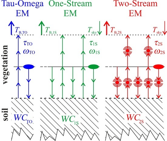
The selection of an adequate EM to be used in a retrieval algorithm is of crucial importance for its performance and applicability range. In this study, three different EM’s are used to simulate brightness temperatures $T_{\mathrm{B},EM}^{p,\theta }$ at nadir angle $\theta$ and Horizontal and Vertical polarizations $p=\left\{\mathrm{H},\mathrm{V}\right\}$ over soils covered with vegetation. The general setup applied with each of the EMs is depicted in Figure 1a. Vegetation is considered as a single homogeneous layer; the soil beneath is represented with an infinite half space exhibiting a rough surface. Symbols and acronyms included in Figure 1a are used in the formulations of the EMs. Section 2.1 outlines two versions of 0^th-order approaches $EM=\left\{\mathrm{TO},1\mathrm{S}\right\}$ used to simulate $T_{\mathrm{B},EM}^{p,\theta }$. It starts with the recap of the so-called “Tau-Omega” (TO) EM ($EM=\mathrm{TO}$) [33] followed by its more complete formulation, developed in [46], and denoted henceforth as One-Stream (1S) EM ($EM=1\mathrm{S}$). The physically most advanced EM investigated here is the Two-Stream (2S) EM ($EM=2\mathrm{S}$) [41] outlined in Section 2.2.

As an outlook to Section 2.1 and Section 2.2, which will explain the different EM’s, Figure 1b sketches the radiative transfer mechanisms considered in $EM=\left\{\mathrm{TO},1\mathrm{S},2\mathrm{S}\right\}$. It depicts how radiation emitted by a volume within the vegetation (solid ellipse) towards the soil contributes to $T_{\mathrm{B},EM}^{p,\theta }$. The TO EM represents this contribution as the radiation reflected at the soil surface and attenuated by the vegetation via absorption and scattering out of the propagating stream. Likewise, the 0^th-order 1S EM represents vegetation volume scattering as a loss mechanism only, but in addition, it considers multiple reflections between the vegetation and the soil surface. Furthermore, 1S EM takes into account downwelling sky brightness temperature $T_{\mathrm{sky}}$ reflected by the scene. The 2S EM goes one step further and includes multiple scattering within vegetation, sketched with the multiple scattering centers (bold dots with concentric circles in Figure 1b).

We will show that the three EMs converge in the case of sparse vegetation. In SMOS and SMAP $EM=\mathrm{TO}$ has been used successfully to retrieve soil water content in the presence of vegetation with low optical depth. Consideration of multiple reflections between vegetation and the soil surface ($EM=1\mathrm{S}$) and multiple scattering in vegetation ($EM=2\mathrm{S}$) becomes increasingly important for retrievals over areas including dense, heavily scattering vegetation, such as forests. In any case, simulating $T_{\mathrm{B},EM}^{p,\theta }$ over vegetated soil allows making the so-called “soft layer” approximation. This implies that refraction and reflection at the upper bound of the vegetation is neglected, because the effective permittivity ${\epsilon }_{\mathrm{v}}$ of the vegetation layer is close to the permittivity of air ${\epsilon }_{\mathrm{air}}=1$ [47]. Consequently, the propagation angle ${\theta }_{\mathrm{v}}$ within the vegetation and the incidence angle ${\theta }_{\mathrm{s}}$ at the soil surface correspond with the nadir observation angle $\theta$, and reflectivity of the air-vegetation interface is assumed as $s_{\mathrm{v}}^{p,\theta }=0$ (Figure 1a).

Generally speaking, $T_{\mathrm{B},EM}^{p,\theta }$ is expressed as the weighted mean of the effective temperatures $T_{\mathrm{s}}$ and $T_{\mathrm{v}}$ of soil (s) and vegetation (v), and the downwelling cold sky $T_{\mathrm{sky}}$:

$$T_{\mathrm{B},EM}^{p,\theta }=T_{\mathrm{s}}\cdot e_{\mathrm{s},EM}^{p,\theta }+T_{\mathrm{v}}\cdot e_{\mathrm{v},EM}^{p,\theta }+T_{\mathrm{sky}}\cdot e_{\mathrm{sky},EM}^{p,\theta }$$

(1)

This formulation is consistent with Kirchhoff’s law of Local Thermodynamic Equilibrium (LTE), and energy conservation requiring $e_{\mathrm{s},EM}^{p,\theta }+e_{\mathrm{v},EM}^{p,\theta }+e_{\mathrm{sky},EM}^{p,\theta }=1$ (Section 1.2 in [4]). Equation (1) is not EM-specific, however, $e_{\mathrm{s},EM}^{p,\theta }$, $e_{\mathrm{v},EM}^{p,\theta }$, $e_{\mathrm{sky},EM}^{p,\theta }$ are EM-dependent emissivities (Kirchhoff coefficients) provided in Section 2.1 and Section 2.2.

Section 2.3 explains the Two-Parameter (2P) retrieval algorithm used to compute $\mathbf{2}{P}_{RC}=(W{C}_{RC},{\tau }_{RC})$ with Retrieval Configuration $RC={\mathrm{TO}}_{{\omega }_{\mathrm{TO}}}$ considered as the “reference” and with the 2S configurations $RC=\left\{2{\mathrm{S}}_{{\omega }_{\mathrm{TO}}},2{\mathrm{S}}_{{\omega }_{2\mathrm{S},\mathrm{eq}}}\right\}$. Section 2.4 outlines the relation between scattering albedos ${\omega }_{\mathrm{TO}}$ used with the “reference” TO EM and corresponding 2S-equivalences ${\omega }_{2\mathrm{S},\mathrm{eq}}({\omega }_{\mathrm{TO}})\ge {\omega }_{\mathrm{TO}}$ adapted for 2S EM. The corresponding transformation ${\omega }_{\mathrm{TO}}\mapsto {\omega }_{2\mathrm{S},\mathrm{eq}}$ is crucial to compute $\mathbf{2}{P}_{RC}=(W{C}_{RC},{\tau }_{RC})$ comparable for TO and 2S Retrieval Configurations $RC$. All configurations $RC=\left\{{\mathrm{TO}}_{{\omega }_{\mathrm{TO}}},2{\mathrm{S}}_{{\omega }_{\mathrm{TO}}},2{\mathrm{S}}_{{\omega }_{2\mathrm{S},\mathrm{eq}}}\right\}$ assume the respective scattering albedos ${\omega }_{\mathrm{TO}}$, ${\omega }_{2\mathrm{S}}={\omega }_{\mathrm{TO}}$ and ${\omega }_{2\mathrm{S}}={\omega }_{2\mathrm{S},\mathrm{eq}}$ as constants. Finally, Section 2.5 provides the essential information on the “Forest Soil Moisture Experiment” (FOSMEX) [8] including the L-band elevation scans $T_{\mathrm{B}}^{p,{\theta }_j}$ measured over a deciduous forest and used in this study to retrieve $\mathbf{2}{P}_{RC}=(W{C}_{RC},{\tau }_{RC})$.

2.1. 0^th-Order Emission Models ($EM=\left\{TO,1S\right\}$)

The current versions of the SMOS and SMAP retrieval algorithms [48,49] applied to estimate soil liquid water content and vegetation optical depth rely on the “Tau-Omega” Emission Model ($EM=\mathrm{TO}$) expressed by Equation (10) in [33]:

$$T_{\mathrm{B},\mathit{EM}}^{p,\theta }=T_{\mathrm{s}}{t}_{\mathit{EM}}^{\theta }(1-s_{\mathrm{s}}^{p,\theta })+(1-{\omega }_{\mathit{EM}})T_{\mathrm{v}}(1-t_{\mathit{EM}}^{\theta })+s_{\mathrm{s}}^{p,\theta }(1-{\omega }_{\mathit{EM}})T_{\mathrm{v}}(1-t_{\mathit{EM}}^{\theta })t_{\mathit{EM}}^{\theta }$$

(2)

As already mentioned (Figure 1b), $T_{\mathrm{B},\mathrm{TO}}^{p,\theta }$ does not properly take into account multiple scattering in vegetation, because TO EM is a 0^th-order solution of the radiative transfer equation. Instead, volume scattering is considered as a loss mechanism only. Furthermore, TO EM ignores multiple reflections between vegetation and the soil surface, it does not include $T_{\mathrm{sky}}$ reflected by the scene.

Transmissivity $t_{EM}^{\theta }$ ($EM=\mathrm{TO}$) of the vegetation layer of thickness $h_{\mathrm{v}}$ is related to its nadir optical depth ${\tau }_{EM}$ via Beer’s law:

$$t_{EM}^{\theta }=\exp (-{\tau }_{EM}/\cos {\theta }_{\mathrm{v}})\mathrm{with}{\theta }_{\mathrm{v}}=\theta \mathrm{and}EM=\left\{\mathrm{TO},1\mathrm{S}\right\}$$

(3)

The absorption coefficient ${\gamma }_{\mathrm{a}}$ and the coefficient ${\gamma }_{\mathrm{b}}$ for scattering of radiation out of the propagating stream define the effective optical depth ${\tau }_{EM}$ and the effective scattering albedo ${\omega }_{EM}$ of the vegetation used in Equation (2):

$${\tau }_{EM}\equiv h_{\mathrm{v}}\cdot ({\gamma }_{\mathrm{a}}+{\gamma }_{\mathrm{b}})\mathrm{and}{\omega }_{EM}\equiv {\gamma }_{\mathrm{b}}/({\gamma }_{\mathrm{a}}+{\gamma }_{\mathrm{b}})\mathrm{with}EM=\left\{\mathrm{TO},1\mathrm{S}\right\}$$

(4)

The TO Kirchhoff coefficients $e_{k,\mathrm{TO}}^{p,\theta }$ (k = s, v, sky) used to represent $T_{\mathrm{B},\mathrm{TO}}^{p,\theta }$ result from rearranging Equation (2) to the form as Equation (1):

$$\begin{array}{l}{e}_{\mathrm{s},\mathrm{TO}}^{p,\theta }=t_{\mathrm{TO}}^{\theta }(1-s_{\mathrm{s}}^{p,\theta })\\ e_{\mathrm{v},\mathrm{TO}}^{p,\theta }=(1-{\omega }_{\mathrm{TO}})(1-t_{\mathrm{TO}}^{\theta })(1+s_{\mathrm{s}}^{p,\theta }{t}_{\mathrm{TO}}^{\theta })\\ e_{\mathrm{sky},\mathrm{TO}}^{p,\theta }=0\end{array}$$

(5)

The neglect of sky $T_{\mathrm{sky}}$ reflected by the scene is seen in $e_{\mathrm{sky},\mathrm{TO}}^{p,\theta }=0$. Accordingly, TO EM is inconsistent with Kirchhoff’s law (Section 1.2 in [4]). The neglect of multiple reflections between the soil surface with reflectivity $s_{\mathrm{s}}^{p,\theta }$ and the vegetation with volume reflectivity $r_{\mathrm{v},\mathrm{TO}}^{p,\theta }$ is apparent from the fact that $e_{k,\mathrm{TO}}^{p,\theta }$ (k = s, v, sky) do not include terms of the form of a geometric series ${{\displaystyle \sum }}_{i=0}^{\infty }{(s_{\mathrm{s}}^{p,\theta }{r}_{\mathrm{v},\mathrm{TO}}^{p,\theta })}^i=1/(1-s_{\mathrm{s}}^{p,\theta }{r}_{\mathrm{v},\mathrm{TO}}^{p,\theta })$. However, both of these physical phenomena neglected in TO EM are considered in 1S EM (Figure 1b), represented by the following 1S Kirchhoff coefficients consistent with Equation (1) in [46]:

$$\begin{array}{l}{e}_{\mathrm{s},1\mathrm{S}}^{p,\theta }=t_{1\mathrm{S}}^{\theta }(1-s_{\mathrm{s}}^{p,\theta })/(1-s_{\mathrm{s}}^{p,\theta }{r}_{\mathrm{v},1\mathrm{S}}^{p,\theta })\\ e_{\mathrm{v},1\mathrm{S}}^{p,\theta }=(1-{\omega }_{1\mathrm{S}})(1-t_{1\mathrm{S}}^{\theta })(1+s_{\mathrm{s}}^{p,\theta }{t}_{1\mathrm{S}}^{\theta }/(1-s_{\mathrm{s}}^{p,\theta }{r}_{\mathrm{v},1\mathrm{S}}^{p,\theta }))\\ e_{\mathrm{sky},1\mathrm{S}}^{p,\theta }=(1-e_{\mathrm{s},1\mathrm{S}}^{p,\theta }-e_{\mathrm{v},1\mathrm{S}}^{p,\theta })\end{array}$$

(6)

Here, volume reflectivity of the vegetation layer is given as:

$$r_{\mathrm{v},1\mathrm{S}}^{p,\theta }={\omega }_{1\mathrm{S}}(1-t_{1\mathrm{S}}^{\theta })$$

(7)

Using $e_{k,1\mathrm{S}}^{p,\theta }$ (k = s, v, sky) in Equation (1) yields $T_{\mathrm{B},1\mathrm{S}}^{p,\theta }$ expressed with 1S EM and is consistent with Kirchhoff’s law ($e_{\mathrm{s},1\mathrm{S}}^{p,\theta }+e_{\mathrm{v},1\mathrm{S}}^{p,\theta }+e_{\mathrm{sky},1\mathrm{S}}^{p,\theta }=1$). Furthermore, multiple reflections between vegetation and the soil surface are considered, but multiple scattering in vegetation is still not included in $EM=1\mathrm{S}$. The latter two issues become increasingly relevant when simulating brightness temperatures over soils covered with dense vegetation, such as forests.

Reflectivities $s_{\mathrm{s}}^{p,\theta }$ of the rough soil surface used in the TO Kirchhoff coefficients $e_{k,\mathrm{TO}}^{p,\theta }$ (Equations (5)) and in the 1S Kirchhoff coefficients $e_{k,1\mathrm{S}}^{p,\theta }$ (Equations (6)) are computed from the respective (specular) Fresnel (F) reflectivities $s_{\mathrm{s},\mathrm{F}}^{p,\theta }$ using the effective permittivity ${\epsilon }_{\mathrm{s}}$ of the soil and the nadir angle ${\theta }_{\mathrm{s}}={\theta }_{\mathrm{v}}=\theta$ at the soil surface (“soft layer” approximation):

$$\begin{array}{l}{s}_{\mathrm{s},\mathrm{F}}^{\mathrm{H},\theta }={\left|\frac{A\sqrt{{\epsilon }_{\mathrm{v}}}-B\sqrt{{\epsilon }_{\mathrm{s}}}}{A\sqrt{{\epsilon }_{\mathrm{v}}}+B\sqrt{{\epsilon }_{\mathrm{s}}}}\right|}^2\mathrm{and}{s}_{\mathrm{s},\mathrm{F}}^{\mathrm{V},\theta }={\left|\frac{A\sqrt{{\epsilon }_{\mathrm{s}}}-B\sqrt{{\epsilon }_{\mathrm{v}}}}{A\sqrt{{\epsilon }_{\mathrm{s}}}+B\sqrt{{\epsilon }_{\mathrm{v}}}}\right|}^2\\ \mathrm{with}{\epsilon }_{\mathrm{v}}\cong {\epsilon }_{\mathrm{air}}=1A=\cos {\theta }_{\mathrm{s}}=\cos \theta B=\sqrt{1-(1-A^2){\epsilon }_{\mathrm{v}}/{\epsilon }_{\mathrm{s}}}\end{array}$$

(8)

Effective soil permittivity ${\epsilon }_{\mathrm{s}}$ serves as the proxy for estimating volumetric soil liquid Water Content $W{C}_{EM}$. The dielectric mixing model [50], using frequency, temperature, and clay content as inputs is used to express ${\epsilon }_{\mathrm{s}}(W{C}_{EM})$.

The effect of soil surface-roughness is simulated with the semi-empirical HQN roughness model [47,51] as is the case in the current SMOS and SMAP retrieval algorithms [48,49].

$$\begin{array}{l}{s}_{\mathrm{s}}^{\mathrm{H},\theta }=\exp (-h_{\mathrm{s}}\cdot {(\cos \theta )}^{n_{\mathrm{s}}^{\mathrm{H}}})\cdot (s_{\mathrm{s},\mathrm{F}}^{\mathrm{H},\theta }\cdot (1-q_{\mathrm{s}})+s_{\mathrm{s},\mathrm{F}}^{\mathrm{V},\theta }\cdot q_{\mathrm{s}})\\ s_{\mathrm{s}}^{\mathrm{V},\theta }=\exp (-h_{\mathrm{s}}\cdot {(\cos \theta )}^{n_{\mathrm{s}}^{\mathrm{V}}})\cdot (s_{\mathrm{s},\mathrm{F}}^{\mathrm{V},\theta }\cdot (1-q_{\mathrm{s}})+s_{\mathrm{s},\mathrm{F}}^{\mathrm{H},\theta }\cdot q_{\mathrm{s}})\end{array}$$

(9)

Typical values of roughness parameters $(h_{\mathrm{s}}, q_{\mathrm{s}}, n_{\mathrm{s}}^{\mathrm{V}}, n_{\mathrm{s}}^{\mathrm{H}})$ proposed for different types of soil surfaces can be found in Table 2 in [36].

Downwelling sky radiance $T_{\mathrm{sky}}$ at L-band is simulated with the empirical approach [52], which uses as inputs air temperature $T_{\mathrm{air}}$ (two meter above ground), elevation Z above sea level, and the nadir angle $\theta$. As the atmosphere is relatively transparent at L-band frequencies, $T_{\mathrm{sky}}$ is small ($\cong 5\mathrm{K})$, and therefore the term $T_{\mathrm{sky}}\cdot e_{\mathrm{sky},EM}^{p,\theta }$ used in Equation (1) to express $T_{\mathrm{B},EM}^{p,\theta }$ is small.

2.2. 1^st-Order Emission Model ($EM=2S$)

A matrix formulation of the multi-layer Two-Stream (2S) EM has been developed as part of the “Microwave Emission Model of Layered Snowpacks” (MEMLS) [40,41]. The single layer configuration of this EM has been used to retrieve snow properties from L-band radiometry [19,20,21,22,23,24]. In the Appendix of [23] the Kirchhoff coefficients of the 2S EM, considering a single absorbing and refractive snow layer, are provided. We use analogous expressions for the 2S Kirchhoff coefficients $e_{k,2\mathrm{S}}^{p,\theta }$ (k = s, v, sky) further simplified for the case of a “soft layer” (i.e., $s_{\mathrm{v}}^{p,\theta }=0$ and ${\theta }_{\mathrm{s}}={\theta }_{\mathrm{v}}=\theta$) generally applicable to compute $T_{\mathrm{B},2\mathrm{S}}^{p,\theta }$ over a soil covered with vegetation using Equation (1):

$$\begin{array}{l}{e}_{\mathrm{s},2\mathrm{S}}^{p,\theta }=t_{\mathrm{v}}^{\theta }(1-s_{\mathrm{s}}^{p,\theta })/(1-s_{\mathrm{s}}^{p,\theta }{r}_{\mathrm{v}}^{\theta })\\ e_{\mathrm{v},2\mathrm{S}}^{p,\theta }=(1-r_{\mathrm{v}}^{\theta }-t_{\mathrm{v}}^{\theta })(1-s_{\mathrm{s}}^{p,\theta }{r}_{\mathrm{v}}^{\theta }+s_{\mathrm{s}}^{p,\theta }{t}_{\mathrm{v}}^{\theta })/(1-s_{\mathrm{s}}^{p,\theta }{r}_{\mathrm{v}}^{\theta })\\ e_{\mathrm{sky},2\mathrm{S}}^{p,\theta }=(1-e_{\mathrm{s},2\mathrm{S}}^{p,\theta }-e_{\mathrm{v},2\mathrm{S}}^{p,\theta })\end{array}$$

(10)

In contrast to $T_{\mathrm{B},EM}^{p,\theta }$ computed with the 0^th-order $EM=\left\{\mathrm{TO},1\mathrm{S}\right\}$ (Section 2.1), $T_{\mathrm{B},2\mathrm{S}}^{p,\theta }$ simulated with the 1^st-order $EM=2\mathrm{S}$ consider multiple scattering in the vegetation. Furthermore, 2S EM is consistent with Kirchhoff’s law ($e_{\mathrm{s},2\mathrm{S}}^{p,\theta }+e_{\mathrm{v},2\mathrm{S}}^{p,\theta }+e_{\mathrm{sky},2\mathrm{S}}^{p,\theta }=1$), and multiple reflections between vegetation and the soil surface are captured by 2S EM (Figure 1b) as is obvious from the terms $1/(1-s_{\mathrm{s}}^{p,\theta }{r}_{\mathrm{v}}^{\theta })$ included in the 2S Kirchhoff coefficients $e_{k,2\mathrm{S}}^{p,\theta }$ (k = s, v, sky).

As was the case with the Kirchhoff coefficients used to represent TO EM (Equations (5)) and 1S EM (Equations (6)), the corresponding $e_{k,2\mathrm{S}}^{p,\theta }$ represent the soil by its surface reflectivity $s_{\mathrm{s}}^{p,\theta }$ expressed by Equations (8) and (9).

Following the derivations outlined in [41], microwave propagation within the vegetation layer is represented by the transmissivity $t_{\mathrm{v}}^{\theta }$ and internal reflectivity $r_{\mathrm{v}}^{\theta }$, both of which take into account multiple reflections between vegetation and the soil surface:

$$\begin{array}{l}{t}_{\mathrm{v}}^{\theta }=t_{\mathrm{v}1}^{\theta }(1-r_{\mathrm{v}\infty }^2)/(1-t_{\mathrm{v}1}^{\theta }{}^2\cdot r_{\mathrm{v}\infty }^2)\\ r_{\mathrm{v}}^{\theta }=r_{\mathrm{v}\infty }(1-t_{\mathrm{v}1}^{\theta }{}^2)/(1-t_{\mathrm{v}1}^{\theta }{}^2\cdot r_{\mathrm{v}\infty }^2)\end{array}$$

(11)

The one-way transmissivity $t_{\mathrm{v}1}^{\theta }$ through the layer with thickness $h_{\mathrm{v}}$, and the reflectivity $r_{\mathrm{v}\infty }$ of a layer with infinite thickness ($h_{\mathrm{v}}\to \infty$) are:

$$t_{\mathrm{v}1}^{\mathsf{\theta }}=\exp (-h_{\mathrm{v}}\cdot {\gamma }_{2\mathrm{S}}/\cos \theta )=\exp (-h_{\mathrm{v}}\cdot \sqrt{{\gamma }_{\mathrm{a}}({\gamma }_{\mathrm{a}}+2{\gamma }_{\mathrm{b}})}/\cos \theta )$$

(12)

and

$$r_{\mathrm{v}\infty }={\gamma }_{\mathrm{b}}/({\gamma }_{\mathrm{a}}+{\gamma }_{\mathrm{b}}+{\gamma }_{2\mathrm{S}})={\gamma }_{\mathrm{b}}/({\gamma }_{\mathrm{a}}+{\gamma }_{\mathrm{b}}+\sqrt{{\gamma }_{\mathrm{a}}({\gamma }_{\mathrm{a}}+2{\gamma }_{\mathrm{b}})})$$

(13)

As is the case in Equation (4), ${\gamma }_{\mathrm{a}}$ is the absorption coefficient and ${\gamma }_{\mathrm{b}}$ is the coefficient for scattering of radiation from its propagation direction into the opposite stream. The vegetation layer’s damping coefficient ${\gamma }_{2\mathrm{S}}$ is:

$${\gamma }_{2\mathrm{S}}=\sqrt{{\gamma }_{\mathrm{a}}({\gamma }_{\mathrm{a}}+2{\gamma }_{\mathrm{b}})}$$

(14)

For the purpose of closest possible notation with TO EM and 1S EM, ${\gamma }_{\mathrm{a}}$ and ${\gamma }_{\mathrm{b}}$ are expressed by the optical depth ${\tau }_{2\mathrm{S}}$ and the scattering albedo ${\omega }_{2\mathrm{S}}$ used with 2S EM. This is achieved by solving the two equations defining ${\tau }_{2\mathrm{S}}$ and ${\omega }_{2\mathrm{S}}$ (in compliance with Equation (4)) by means of ${\gamma }_{\mathrm{a}}$ and ${\gamma }_{\mathrm{b}}$:

$${\tau }_{2\mathrm{S}}\equiv h_{\mathrm{v}}\cdot ({\gamma }_{\mathrm{a}}+{\gamma }_{\mathrm{b}})\mathrm{and}{\omega }_{2\mathrm{S}}\equiv {\gamma }_{\mathrm{b}}/({\gamma }_{\mathrm{a}}+{\gamma }_{\mathrm{b}})$$

(15)

The result is:

$${\gamma }_{\mathrm{a}}={\tau }_{2\mathrm{S}}\cdot (1-{\omega }_{2\mathrm{S}})/h_{\mathrm{v}}\mathrm{and}{\gamma }_{\mathrm{b}}={\tau }_{2\mathrm{S}}\cdot {\omega }_{2\mathrm{S}}/h_{\mathrm{v}}$$

(16)

Now, using ${\gamma }_{\mathrm{a}}({\tau }_{2\mathrm{S}},{\omega }_{2\mathrm{S}})$ and ${\gamma }_{\mathrm{b}}({\tau }_{2\mathrm{S}},{\omega }_{2\mathrm{S}})$ in Equations (12)–(14) yields $t_{\mathrm{v}1}^{\theta }$ and $r_{\mathrm{v}\infty }$ as functions of ${\tau }_{2\mathrm{S}}$ and ${\omega }_{2\mathrm{S}}$ and are independent of the vegetation layer thickness $h_{\mathrm{v}}$:

$$t_{\mathrm{v}1}^{\theta }=\exp (-{\tau }_{2\mathrm{S}}\sqrt{1-{\omega }_{2\mathrm{S}}^2}/\cos \theta )\mathrm{and}{r}_{\mathrm{v}\infty }={\omega }_{2\mathrm{S}}/(1+\sqrt{1-{\omega }_{2\mathrm{S}}^2})$$

(17)

Inserting $t_{\mathrm{v}1}^{\theta }$ and $r_{\mathrm{v}\infty }$ in Equation (11) yields the transitivity $t_{\mathrm{v}}^{\theta }$ and the reflectivity $r_{\mathrm{v}}^{\theta }$ of the vegetation layer expressed with ${\tau }_{2\mathrm{S}}$ and ${\omega }_{2\mathrm{S}}$:

$$\begin{array}{l}{t}_{\mathrm{v}}^{\theta }=\frac{2\cdot \exp ({\tau }_{2\mathrm{S}}\sqrt{1-{\omega }_{2\mathrm{S}}^2}/\cos \theta )\cdot \left[1-{\omega }_{2\mathrm{S}}^2+\sqrt{1-{\omega }_{2\mathrm{S}}^2}\right]}{\exp (2{\tau }_{2\mathrm{S}}\sqrt{1-{\omega }_{2\mathrm{S}}^2}/\cos \theta )\cdot \left[2-{\omega }_{2\mathrm{S}}^2+2\sqrt{1-{\omega }_{2\mathrm{S}}^2}\right]-{\omega }_{2\mathrm{S}}^2}\\ r_{\mathrm{v}}^{\theta }=\frac{{\omega }_{2\mathrm{S}}\cdot \left[\exp (2{\tau }_{2\mathrm{S}}\sqrt{1-{\omega }_{2\mathrm{S}}^2}/\cos \theta )-1\right]\cdot \left[1+\sqrt{1-{\omega }_{2\mathrm{S}}^2}\right]}{\exp (2{\tau }_{2\mathrm{S}}\sqrt{1-{\omega }_{2\mathrm{S}}^2}/\cos \theta )\cdot \left[2-{\omega }_{2\mathrm{S}}^2+2\sqrt{1-{\omega }_{2\mathrm{S}}^2}\right]-{\omega }_{2\mathrm{S}}^2}\end{array}$$

(18)

Finally, using Equations (18) together with the soil reflectivities $s_{\mathrm{s}}^{p,\theta }$ (Equations (8) and (9)) in Equations (10) for the 2S Kirchhoff coefficients $e_{k,2\mathrm{S}}^{p,\theta }$ (k = s, v, sky) yields $T_{\mathrm{B},2\mathrm{S}}^{p,\theta }$ expressed with Equation (1).

2.3. Retrieval Algorithm

Retrievals $\mathbf{2}{P}_{RC}=(W{C}_{RC},{\tau }_{RC})$ are derived from $T_{\mathrm{B}}^{p,{\theta }_j}$ elevation scans. The retrieved values are computed by tuning $W{C}_{RC}$ and ${\tau }_{RC}$ to reach an optimal match between $T_{\mathrm{B},EM}^{p,{\theta }_j}$ simulated with $EM=\mathrm{TO}$ or $EM=2\mathrm{S}$ and observed $T_{\mathrm{B}}^{p,{\theta }_j}$. To this aim the following Cost-Function ($CF$) is minimized:

$$CF={{\displaystyle \sum }}_{p,{\theta }_j}{(T_{\mathrm{B}}^{p,{\theta }_j}-T_{\mathrm{B},EM}^{p,{\theta }_j})}^2$$

(19)

Summation is performed over the nadir angles ${\theta }_j$ and $p=\left\{\mathrm{H},\mathrm{V}\right\}$ included in the elevation scan $T_{\mathrm{B}}^{p,{\theta }_j}$. A global numerical optimizer is used to compute the minimum of $CF$ in the two-dimensional $(W{C}_{RC},{\tau }_{RC})$ parameter space restricted to $0 {\mathrm{m}}^3{\mathrm{m}}^{-3}\le W{C}_{RC}\le 1{\mathrm{m}}^3{\mathrm{m}}^{-3}$ and $0 \le {\tau }_{RC}\le 3$. Other parameters involved in the simulation of $T_{\mathrm{B},EM}^{p,{\theta }_j}$ (such as ${\omega }_{EM}$, $T_{\mathrm{s}}=T_{\mathrm{v}}$, $\left\{h_{\mathrm{s}},q_{\mathrm{s}},n_{\mathrm{s}}^{\mathrm{V}},n_{\mathrm{s}}^{\mathrm{H}}\right\}$) are considered constant during the minimization.

The retrieval approach is applied to achieve $\mathbf{2}{P}_{RC}=(W{C}_{RC},{\tau }_{RC})$ from synthetic (Section 3.2) and experimental (Section 3.3) $T_{\mathrm{B}}^{p,{\theta }_j}$. Thereby, the “reference” TO Retrieval Configuration $RC={\mathrm{TO}}_{{\omega }_{\mathrm{TO}}}$ and the two 2S configurations $RC=\left\{2{\mathrm{S}}_{{\omega }_{\mathrm{TO}}},2{\mathrm{S}}_{{\omega }_{2\mathrm{S},\mathrm{eq}}}\right\}$ are investigated:

• $RC={\mathrm{TO}}_{{\omega }_{\mathrm{TO}}}$: “reference” TO EM with TO scattering albedo ${\omega }_{\mathrm{TO}}=$ constant.
• $RC=2{\mathrm{S}}_{{\omega }_{\mathrm{TO}}}$: 2S EM with 2S scattering albedo ${\omega }_{2\mathrm{S}}=$ constant $={\omega }_{\mathrm{TO}}$.
• $RC=2{\mathrm{S}}_{{\omega }_{2\mathrm{S},\mathrm{eq}}}$: 2S EM with 2S-equivalent scattering albedo ${\omega }_{2\mathrm{S},\mathrm{eq}}=$ constant $>{\omega }_{\mathrm{TO}}$.

$RC={\mathrm{TO}}_{{\omega }_{\mathrm{TO}}}$ is considered as the “reference” configuration, because it uses TO EM implemented in operational SMOS and SMAP retrieval algorithms with constant ${\omega }_{\mathrm{TO}}$ to simulate $T_{\mathrm{B},EM}^{p,{\theta }_j}=T_{\mathrm{B},\mathrm{TO}}^{p,{\theta }_j}$ used in the $CF$ (Equation (19)). 2S configurations $RC=\left\{2{\mathrm{S}}_{{\omega }_{\mathrm{TO}}},2{\mathrm{S}}_{{\omega }_{2\mathrm{S},\mathrm{eq}}}\right\}$ use 2S EM to simulate $T_{\mathrm{B},EM}^{p,{\theta }_j}=T_{\mathrm{B},2\mathrm{S}}^{p,{\theta }_j}$ used in the $CF$ (Equation (19)). The difference between the two 2S configurations is that $RC=2{\mathrm{S}}_{{\omega }_{\mathrm{TO}}}$ assumes the same constant value ${\omega }_{2\mathrm{S}}={\omega }_{\mathrm{TO}}$ for vegetation scattering albedo as is used with TO EM, while $RC=2{\mathrm{S}}_{{\omega }_{2\mathrm{S},\mathrm{eq}}}$ considers 2S-equivalent scattering albedo ${\omega }_{2\mathrm{S},\mathrm{eq}}\ge {\omega }_{\mathrm{TO}}$ as constant throughout the retrieval. Because ${\omega }_{2\mathrm{S},\mathrm{eq}}\ne {\omega }_{\mathrm{TO}}$, computation of 2S-equivalent scattering albedo ${\omega }_{2\mathrm{S},\mathrm{eq}}$ is a basic requirement to achieve retrievals $\mathbf{2}{P}_{RC}=(W{C}_{RC},{\tau }_{RC})$ with $RC=2{\mathrm{S}}_{{\omega }_{2\mathrm{S},\mathrm{eq}}}$, which are comparable against $\mathbf{2}{P}_{RC}=(W{C}_{RC},{\tau }_{RC})$ using $RC={\mathrm{TO}}_{{\omega }_{\mathrm{TO}}}$.

2.4. 2S-Equivalent Scattering Albedo

SMOS retrievals $\mathbf{2}{P}_{RC}=(W{C}_{RC},{\tau }_{RC})$ using $RC={\mathrm{TO}}_{{\omega }_{\mathrm{TO}}}$ over forests assume ${\omega }_{\mathrm{TO}}\approx 0.08$ (Table 1 in [36]) as constant. This value was estimated by fitting $T_{\mathrm{B},\mathrm{TO}}^{p,\theta }$ to numerically simulated brightness temperatures over forests represented by dielectric cylinders of different sizes and orientations [5,6]. Assuming 2S EM would have been selected for SMOS retrievals from the beginning of the mission, the same approach would have been used to calibrate ${\omega }_{2\mathrm{S}}$ for forests. However, this was not the case when SMOS was launched. Therefore, we choose an alternative method to estimate 2S-equivalences ${\omega }_{2\mathrm{S},\mathrm{eq}}$ from calibrated ${\omega }_{\mathrm{TO}}$ used with the “reference” TO EM. Ultimately, our approach yields a Fast Model (FM) to compute ${\omega }_{2\mathrm{S},\mathrm{eq}}={\omega }_{2\mathrm{S},\mathrm{eq}}^{\mathrm{FM}}({\omega }_{\mathrm{TO}})$ mandatory to achieve $\mathbf{2}{P}_{RC}=(W{C}_{RC},{\tau }_{RC})$ which are comparable for TO and 2S retrieval configurations on a fair basis (Section 3).

As a consequence of the varying degrees of simplification made in the solution of the radiative transfer equation to yield TO EM and 2S EM, there exists crosstalk between the model parameters $({\tau }_{EM},{\omega }_{EM},W{C}_{EM})$ used with $EM=\mathrm{TO}$ and $EM=2\mathrm{S}$. Accordingly, the parameter transformation $({\tau }_{\mathrm{TO}},{\omega }_{\mathrm{TO}},W{C}_{\mathrm{TO}})\mapsto ({\tau }_{2\mathrm{S},\mathrm{eq}},{\omega }_{2\mathrm{S},\mathrm{eq}},W{C}_{2\mathrm{S},\mathrm{eq}})$ is not obvious, but is a necessary step towards the derivation of the FM ${\omega }_{2\mathrm{S},\mathrm{eq}}^{\mathrm{FM}}({\omega }_{\mathrm{TO}})$.

The approach taken to compute transformations $({\tau }_{\mathrm{TO}},{\omega }_{\mathrm{TO}},W{C}_{\mathrm{TO}})\mapsto ({\tau }_{2\mathrm{S},\mathrm{eq}},{\omega }_{2\mathrm{S},\mathrm{eq}},W{C}_{2\mathrm{S},\mathrm{eq}})$ is based on the assumption that 2S system (sys) emissivities $e_{2\mathrm{S},\mathrm{sys}}^{p,{\theta }_j}$ computed for $({\tau }_{2\mathrm{S},\mathrm{eq}},{\omega }_{2\mathrm{S},\mathrm{eq}},W{C}_{2\mathrm{S},\mathrm{eq}})$ must be as similar as possible to TO system emissivities $e_{\mathrm{TO},\mathrm{sys}}^{p,{\theta }_j}$ computed for $({\tau }_{\mathrm{TO}},{\omega }_{\mathrm{TO}},W{C}_{\mathrm{TO}})$. Accordingly, 2S-equivalent parameters $({\tau }_{2\mathrm{S},\mathrm{eq}},{\omega }_{2\mathrm{S},\mathrm{eq}},W{C}_{2\mathrm{S},\mathrm{eq}})$ are computed by minimizing the following Cost-Function $CF$:

$$CF={{\displaystyle \sum }}_{p,{\theta }_j}{(e_{\mathrm{TO},\mathrm{sys}}^{p,{\theta }_j}-e_{2\mathrm{S},\mathrm{sys}}^{p,{\theta }_j})}^2$$

(20)

Assuming $T_{\mathrm{v}}=T_{\mathrm{s}}$, TO emissivities $e_{\mathrm{TO},\mathrm{sys}}^{p,{\theta }_j}=e_{\mathrm{s},\mathrm{TO}}^{p,{\theta }_j}+e_{\mathrm{v},\mathrm{TO}}^{p,{\theta }_j}$ and 2S emissivities $e_{2\mathrm{S},\mathrm{sys}}^{p,{\theta }_j}=e_{\mathrm{s},2\mathrm{S}}^{p,{\theta }_j}+e_{\mathrm{v},2\mathrm{S}}^{p,{\theta }_j}$ are expressed with the Kirchhoff coefficients given by Equations (5) and (10), respectively. Summation in Equation (20) is performed over ${\theta }_j=\left\{0°,5°,\dots ,60°\right\}$. and over $p=\left\{\mathrm{H},\mathrm{V}\right\}$. Soil surface-roughness is parameterized with $(h_{\mathrm{s}},q_{\mathrm{s}},n_{\mathrm{s}}^{\mathrm{V}},n_{\mathrm{s}}^{\mathrm{H}})=(1,0,0,0)$ and its clay content is assumed as $0.16{\mathrm{kg}\mathrm{kg}}^{-1}$. A numerical optimizer is used to find the global minimum of the $CF$ in the three-dimensional 2S parameter space without any restrictions.

As mentioned, 2S-equivalences ${\omega }_{2\mathrm{S},\mathrm{eq}}$ depend on all of the three TO parameters $({\tau }_{\mathrm{TO}},{\omega }_{\mathrm{TO}},W{C}_{\mathrm{TO}})$ due to parameter crosstalk. However, ${\omega }_{2\mathrm{S},\mathrm{eq}}({\tau }_{\mathrm{TO}},{\omega }_{\mathrm{TO}},W{C}_{\mathrm{TO}})$ computed for $W{C}_{\mathrm{TO}}$ and ${\tau }_{\mathrm{TO}}$ over realistic ranges show that ${\omega }_{2\mathrm{S},\mathrm{eq}}$ is predominantly sensitive to ${\omega }_{\mathrm{TO}}$, while sensitivities with respect to ${\tau }_{\mathrm{TO}}$ and $W{C}_{\mathrm{TO}}$ are of second order. This suggests that ${\omega }_{2\mathrm{S},\mathrm{eq}}$ can be approximated exclusively from ${\omega }_{\mathrm{TO}}$, while uncertainty $\mathsf{\sigma }{\omega }_{2\mathrm{S},\mathrm{eq}}$ introduced via the omission of the dependencies on ${\tau }_{\mathrm{TO}}$ and $W{C}_{\mathrm{TO}}$ can be estimated by considering meaningful ranges for ${\tau }_{\mathrm{TO}}$ and $W{C}_{\mathrm{TO}}$.

To be specific, ${\omega }_{2\mathrm{S},\mathrm{eq}}({\omega }_{\mathrm{TO}})$ is estimated from sets of $J\cdot K$ values of ${\omega }_{2\mathrm{S},\mathrm{eq}}({\tau }_{\mathrm{TO},j},{\omega }_{\mathrm{TO}},W{C}_{\mathrm{TO},k})$ averaged over the $j=1,\dots ,J=60$ values of ${\tau }_{\mathrm{TO},j}=\left\{0.00,0.05,\dots ,1.50\right\}$ and the $k=1,\dots ,K=60$ values of $W{C}_{\mathrm{TO},k}=\left\{0.01,0.02,\dots ,0.60\right\}{\mathrm{m}}^3{\mathrm{m}}^{-3}$.

$${\omega }_{2\mathrm{S},\mathrm{eq}}({\omega }_{\mathrm{TO}})=\frac{1}{J\cdot K}{\displaystyle \sum }_{j,k}^{J,K}{\omega }_{2\mathrm{S},\mathrm{eq}}({\tau }_{\mathrm{TO},j},{\omega }_{\mathrm{TO}},W{C}_{\mathrm{TO},k})$$

(21)

Uncertainty $\mathsf{\sigma }{\omega }_{2\mathrm{S},\mathrm{eq}}({\omega }_{\mathrm{TO}})$ of ${\omega }_{2\mathrm{S},\mathrm{eq}}({\omega }_{\mathrm{TO}})$ is computed as the standard deviation of the set of ${\omega }_{2\mathrm{S},\mathrm{eq}}({\tau }_{\mathrm{TO},j},{\omega }_{\mathrm{TO}},W{C}_{\mathrm{TO},k})$ for a given ${\omega }_{\mathrm{TO}}$:

$$\mathsf{\sigma }{\omega }_{2\mathrm{S},\mathrm{eq}}({\omega }_{\mathrm{TO}})=\sqrt{\frac{1}{J\cdot K}{\displaystyle \sum }_{j,k}^{J,K}{\left[{\omega }_{2\mathrm{S},\mathrm{eq}}({\tau }_{\mathrm{TO},j},{\omega }_{\mathrm{TO}},W{C}_{\mathrm{TO},k})-{\omega }_{2\mathrm{S},\mathrm{eq}}({\omega }_{\mathrm{TO}})\right]}^2}$$

(22)

The dots in Figure 2 show ${\omega }_{2\mathrm{S},\mathrm{eq}}({\omega }_{\mathrm{TO}})$ and the gray-shaded area represents its uncertainty $\mathsf{\sigma }{\omega }_{2\mathrm{S},\mathrm{eq}}({\omega }_{\mathrm{TO}})$ caused by crosstalk of ${\tau }_{\mathrm{TO}}$ and $W{C}_{\mathrm{TO}}$. As can be seen, $\mathsf{\sigma }{\omega }_{2\mathrm{S},\mathrm{eq}}({\omega }_{\mathrm{TO}})$ are much smaller than ${\omega }_{2\mathrm{S},\mathrm{eq}}({\omega }_{\mathrm{TO}})$, especially for ${\omega }_{\mathrm{TO}}<0.10$ realistic of natural vegetation [36], which justifies the expression of ${\omega }_{2\mathrm{S},\mathrm{eq}}({\omega }_{\mathrm{TO}})$ exclusively as a function ${\omega }_{\mathrm{TO}}$.

As explained, computing ${\omega }_{2\mathrm{S},\mathrm{eq}}({\omega }_{\mathrm{TO}})$ for a given ${\omega }_{\mathrm{TO}}$ requires computation of $60\cdot 60=3600$ ${\omega }_{2\mathrm{S},\mathrm{eq}}({\tau }_{\mathrm{TO},j},{\omega }_{\mathrm{TO}},W{C}_{\mathrm{TO},k})$, each of which involves the optimization of the $CF$ defined by Equation (20). Accordingly, the computational cost is too high for a direct implementation of ${\omega }_{2\mathrm{S},\mathrm{eq}}({\omega }_{\mathrm{TO}})$ in a retrieval algorithm. Therefore, ${\omega }_{2\mathrm{S},\mathrm{eq}}({\omega }_{\mathrm{TO}})$ is represented with a Fast Model (FM) ${\omega }_{2\mathrm{S},\mathrm{eq}}^{\mathrm{FM}}({\omega }_{\mathrm{TO}})$ ultimately used to achieve retrievals $\mathbf{2}{P}_{RC}=(W{C}_{RC},{\tau }_{RC})$ with $RC=2{\mathrm{S}}_{{\omega }_{2\mathrm{S},\mathrm{eq}}}$ considering ${\omega }_{2\mathrm{S},\mathrm{eq}}={\omega }_{2\mathrm{S},\mathrm{eq}}^{\mathrm{FM}}({\omega }_{\mathrm{TO}})$ as constant.

This FM is formulated as a 4^th-order polynomial considering the side constraints: ${{\omega }_{2\mathrm{S},\mathrm{eq}}^{\mathrm{FM}}|}_{{\omega }_{\mathrm{TO}}=0}=0$, ${{\omega }_{2\mathrm{S},\mathrm{eq}}^{\mathrm{FM}}|}_{{\omega }_{\mathrm{TO}}=1}=1$, and ${d{\omega }_{2\mathrm{S},\mathrm{eq}}^{\mathrm{FM}}/d{\omega }_{\mathrm{TO}}|}_{{\omega }_{\mathrm{TO}}=1}=0$:

$${\omega }_{2\mathrm{S},\mathrm{eq}}^{\mathrm{FM}}({\omega }_{\mathrm{TO}})=A{\omega }_{\mathrm{TO}}+B{\omega }_{\mathrm{TO}}^2+(4-3A-2B){\omega }_{\mathrm{TO}}^3+(2A+B-3){\omega }_{\mathrm{TO}}^4$$

(23)

The fitting parameters yielding ${\omega }_{2\mathrm{S},\mathrm{eq}}^{\mathrm{FM}}({\omega }_{\mathrm{TO}})$, shown with the solid line in Figure 2, are $A=1.45644$ and $B=1.52340$.

2.5. Ground-Based Experimental Datasets

The retrievals $\mathbf{2}{P}_{RC}=(W{C}_{RC},{\tau }_{RC})$ presented in Section 3.3 are derived from elevation scans $T_{\mathrm{B}}^{p,{\theta }_j}$ of L-band brightness temperatures measured during the “Forest Soil Moisture Experiment” (FOSMEX) [8] performed between January 2005 and January 2006 at a forest site at the Research Centre Jülich (FZJ, Germany). This deciduous forest comprised oak, birch, and beech in similar proportions. Tree age was between 40 and 80 years, and the average crown height was approximately 24 m. Column density of dry canopy biomass was $~15{\mathrm{kg}\mathrm{m}}^{-2}$, and column density of the fresh leaves was $~1.14{\mathrm{kg}\mathrm{m}}^{-2}$ for the fully foliated canopy [7].

Brightness temperatures $T_{\mathrm{B}}^{p,{\theta }_j}$ were measured by the L-band radiometer ELBARA [53] (the precursor of ELBARA-II [54] used for SMOS calibration and validation purposes) attached to an elevation scanner mounted on a 100-m platform of the meteorological tower located within the forest stand. Hourly elevation scans $T_{\mathrm{B}}^{p,{\theta }_j}$, each of which including nadir angles ${\theta }_j=\left\{46°,50°,54°,58°,62°,66°\right\}$, were acquired at polarization $p=\left\{\mathrm{H},\mathrm{V}\right\}$. We only use $T_{\mathrm{B}}^{p,{\theta }_j}$ scans including ${\theta }_j=\left\{46°,50°,54°,58°\right\}$ shown in Figure 3c,d, for $p=\mathrm{H}$ and $p=\mathrm{V}$, respectively. The angles ${\theta }_j=\left\{62°,66°\right\}$ are excluded because these observations include radiative contributions from close to the horizon considering the $-6\mathrm{dB}$ sensitivity of $~\pm 9°$ of the antenna around its main direction (Figure 9 in [54]). Furthermore, only morning measurements (4 a.m.–8 a.m.) are selected to ensure $T_{\mathrm{v}}\cong T_{\mathrm{s}}$.

The magenta squares in Figure 3a show forest soil temperatures $T_{\mathrm{s}}$ estimated as the average of eight thermistor readings performed $~5\mathrm{cm}$ below the litter layer within an area of $~10\mathrm{m}\times 10\mathrm{m}$ Precipitation was measured at the 20-m platform of the meteorological tower and aggregated to 12-h averages $P$ (blue columns) representative of the diurnal time-window 6 p.m.–6 a.m. to improve the chances for synchronicity with the morning measurements $T_{\mathrm{B}}^{p,{\theta }_j}$ performed between 4 a.m.–8 a.m. Relative Foliation $RF$ of the forest canopy (green line in Figure 3b) was estimated from photos regularly taken from below the canopy. In-situ soil-water content $W{C}_{\mathrm{in}-\mathrm{situ}}$ was estimated with Time Domain Reflectometer (TDR) probes installed horizontally $~5\mathrm{cm}$ below the litter layer within an area of $~10\mathrm{m}\times 10\mathrm{m}$ The dielectric mixing model [50] assuming clay content $0.16{\mathrm{kg}\mathrm{kg}}^{-1}$ and in-situ $T_{\mathrm{s}}$ is used to compute areal means $W{C}_{\mathrm{in}-\mathrm{situ}}$ (black stars in Figure 3b) of volumetric liquid water content of the forest soil surface.

Coupled time dependencies of $W{C}_{\mathrm{in}-\mathrm{situ}}$ (black stars in Figure 3b) and precipitation $P$ (blue columns in Figure 3a) are apparent. Nonetheless, responses of $T_{\mathrm{B}}^{p,{\theta }_j}$ with respect to $W{C}_{\mathrm{in}-\mathrm{situ}}$ remain elusive, and only noticeable during the two strongest precipitation periods taking place at around the 1st and the 29th of July 2005. However, drops of $T_{\mathrm{B}}^{p,{\theta }_j}$ synchronous with these most intense precipitation events are ambiguous. They are explained by lowered effective temperature of the forest soil due to rain, and due to the increased real part of effective permittivity of soil reducing its emissivity. Of course, rain also increases the imaginary part of vegetation effective permittivity via water droplets forming at the leaf surfaces, which in turn increases canopy attenuation. However, corresponding increased vegetation optical depth increases $T_{\mathrm{B}}^{p,{\theta }_j}$ less than the above-mentioned effects lowering $T_{\mathrm{B}}^{p,{\theta }_j}$ as the result of rain.

Observed decreases of $T_{\mathrm{B}}^{p,{\theta }_j}$ contemporaneous with $P$ do not exceed $~5\mathrm{K}$. The rather small response of L-band brightness temperatures induced by artificially sprinkling the forest ground was demonstrated in our previous work [8]. The respective “irrigation experiment” performed on the 5th October 2005 showed that L-band brightness temperatures are reduced by $\lesssim 2\mathrm{K}$ within less than $~2\mathrm{h}$ after sprinkling the forest ground with $~45{\mathrm{mm}\mathrm{h}}^{-1}$ for 1 h. The small response of brightness temperatures, as well as its swift subsiding was attributed to leaf litter at the forest soil. On the one hand, the litter layer plays a crucial role in the microwave radiative transfer [55], mostly via impedance matching, reducing the sensitivity of brightness temperature with respect to the water content of the soil below the litter. On the other hand, water in the litter layer drains quickly and is largely decoupled from $W{C}_{\mathrm{in}-\mathrm{situ}}$ measured $~5\mathrm{cm}$ below the litter and serving as references for the comparison with microwave measurements.

The seasonal patterns of $T_{\mathrm{B}}^{p,{\theta }_j}$ shown in Figure 3c,d follow the evolution of the foliation $RF$ (green line in Figure 3b), and at the same time the seasonality of in-situ soil temperature $T_{\mathrm{s}}$ (magenta squares in Figure 3a). Again, this ambiguity raises the question to what extent information on forest state parameters can be retrieved from $T_{\mathrm{B}}^{p,{\theta }_j}$. Section 3.3 will shed further light on the challenge of retrieving $\mathbf{2}{P}_{RC}=(W{C}_{RC},{\tau }_{RC})$ from L-band $T_{\mathrm{B}}^{p,{\theta }_j}$ measured over a deciduous forest with leaf litter covering the soil.

3. Results and Discussion

3.1. Brightness Temperatures Simulated with EM = {TO,1S,2S}

The goal of this section is to analyze differences $\mathsf{\Delta }{T}_{\mathrm{B},1\mathrm{S}-\mathrm{TO}}^{p,\theta }(\tau ,\omega )$ between brightness temperatures $T_{\mathrm{B},EM}^{p,\theta }(\tau ,\omega )$ simulated with $EM=1\mathrm{S}$ and the “reference” $EM=\mathrm{TO}$, and differences $\mathsf{\Delta }{T}_{\mathrm{B},2\mathrm{S}-\mathrm{TO}}^{p,\theta }(\tau ,\omega )$ between $T_{\mathrm{B},EM}^{p,\theta }(\tau ,\omega )$ simulated with $EM=2\mathrm{S}$ and $EM=\mathrm{TO}$:

$$\begin{array}{l}\mathsf{\Delta }{T}_{\mathrm{B},1\mathrm{S}-\mathrm{TO}}^{p,\theta }(\tau ,\omega )\equiv T_{\mathrm{B},1\mathrm{S}}^{p,\theta }(\tau ,\omega )-T_{\mathrm{B},\mathrm{TO}}^{p,\theta }(\tau ,\omega )\\ \mathsf{\Delta }{T}_{\mathrm{B},2\mathrm{S}-\mathrm{TO}}^{p,\theta }(\tau ,\omega )\equiv T_{\mathrm{B},2\mathrm{S}}^{p,\theta }(\tau ,\omega )-T_{\mathrm{B},\mathrm{TO}}^{p,\theta }(\tau ,\omega )\end{array}$$

(24)

Simulated $T_{\mathrm{B},\mathrm{TO}}^{p,\theta }(\tau ,\omega )$, $T_{\mathrm{B},1\mathrm{S}}^{p,\theta }(\tau ,\omega )$, and $T_{\mathrm{B},2\mathrm{S}}^{p,\theta }(\tau ,\omega )$ assume consistent optical depth $\tau ={\tau }_{\mathrm{TO}}={\tau }_{1\mathrm{S}}={\tau }_{2\mathrm{S}}$, scattering albedo $\omega ={\omega }_{\mathrm{TO}}={\omega }_{1\mathrm{S}}={\omega }_{2\mathrm{S}}$, soil water content $WC=W{C}_{\mathrm{TO}}=W{C}_{1\mathrm{S}}=W{C}_{2\mathrm{S}}=0.2 {\mathrm{m}}^3{\mathrm{m}}^{-3}$, and $\theta =40°$. Further parameter values used commonly in the EMs are listed in

Table 1. Parameters used in the “reference” TO EM and the EMs 1S and 2S used to compute differences $\mathsf{\Delta }{T}_{\mathrm{B},1\mathrm{S}-\mathrm{TO}}^{p,40°}(\tau ,\omega )$ and $\mathsf{\Delta }{T}_{\mathrm{B},2\mathrm{S}-\mathrm{TO}}^{p,40°}(\tau ,\omega )$ shown in Figure 4. Same parameters are used to compute $\mathsf{\Delta }W{C}_{\mathrm{TO}-RC}$ and $\mathsf{\Delta }{\tau }_{\mathrm{TO}-RC}$ (Figure 5) between retrievals $\mathbf{2}{P}_{RC}=(W{C}_{RC},{\tau }_{RC})$ achieved with the “reference” Retrieval Configuration $RC={\mathrm{TO}}_{{\omega }_{\mathrm{TO}}}$ and $RC=\left\{2{\mathrm{S}}_{{\omega }_{\mathrm{TO}}},2{\mathrm{S}}_{{\omega }_{2\mathrm{S},\mathrm{eq}}}\right\}$ defined in Section 2.3.

EM Parameter
Symbol	Meaning	Value
$p$	polarization	$\left\{\mathrm{H},\mathrm{V}\right\}$
$f$	frequency	$1.4\mathrm{GHz}$
$T_{\mathrm{s}}=T_{\mathrm{v}}=T_{\mathrm{air}}$	physical temp. of soil, veg., and air	$300\mathrm{K}$
$clay$	soil clay content	$0.16{\mathrm{kg}\mathrm{kg}}^{-1}$
$\left\{h_{\mathrm{s}},q_{\mathrm{s}},n_{\mathrm{s}}^{\mathrm{V}},n_{\mathrm{s}}^{\mathrm{H}}\right\}$	HQN roughness parameters	$\left\{1,0,0,0\right\}$
$Z$	altitude above sea level	$0.400\mathrm{km}$

. Figure 4a,b show contour plots of $\mathsf{\Delta }{T}_{\mathrm{B},1\mathrm{S}-\mathrm{TO}}^{p,\theta }(\tau ,\omega )$ and $\mathsf{\Delta }{T}_{\mathrm{B},2\mathrm{S}-\mathrm{TO}}^{p,\theta }(\tau ,\omega )$, respectively, for ranges $0.0\le \tau \le 1.5$ and $0.0\le \omega \le 1.0$. Blue dashed contours are for $p=\mathrm{H}$ and red solid contours are for $p=\mathrm{V}$.

The $\mathsf{\Delta }{T}_{\mathrm{B},1\mathrm{S}-\mathrm{TO}}^{p,40°}(\tau ,\omega )$ shown in Figure 4a are always positive and increase with increasing $\tau$ and $\omega$, showing that $T_{\mathrm{B},1\mathrm{S}}^{p,\theta }(\tau ,\omega )$ simulated with 1S EM is consistently larger than $T_{\mathrm{B},\mathrm{TO}}^{p,\theta }(\tau ,\omega )$ simulated with TO EM. This is due to multiple reflections between the soil surface and vegetation neglected in TO EM but considered in 1S EM (Figure 1b). Consideration of these multiple reflections becomes increasingly important for dense vegetation with increased volume reflectivity $r_{\mathrm{v},1\mathrm{S}}^{p,\theta }$ (Equation (7)). $T_{\mathrm{sky}}$ reflected by the scene, considered in 1S EM but ignored in TO EM (Figure 1b), further increases $\mathsf{\Delta }{T}_{\mathrm{B},1\mathrm{S}-\mathrm{TO}}^{p,40°}(\tau ,\omega )$. However, due to $T_{\mathrm{sky}}\approx 5 \mathrm{K}$ and low scene reflectivity $(1-e_{\mathrm{s},1\mathrm{S}}^{p,\theta }-e_{\mathrm{v},1\mathrm{S}}^{p,\theta })=e_{\mathrm{sky},1\mathrm{S}}^{p,\theta }\ll 1$ the contribution of $T_{\mathrm{sky}}\cdot e_{\mathrm{sky},1\mathrm{S}}^{p,\theta }$ (Equation (1)) to $T_{\mathrm{B},1\mathrm{S}}^{p,\theta }(\tau ,\omega )$ is small compared to the increase associated with multiple reflections between vegetation and the soil surface.

For $\tau =0$ and/or $\omega =0$ the $\mathsf{\Delta }{T}_{\mathrm{B},1\mathrm{S}-\mathrm{TO}}^{p,40°}(\tau ,\omega )$-isolines as well as the $\mathsf{\Delta }{T}_{\mathrm{B},2\mathrm{S}-\mathrm{TO}}^{p,\theta }(\tau ,\omega )$-isolines approach zero. This corroborates with the fact that all the $EM=\left\{\mathrm{TO},1\mathrm{S},2\mathrm{S}\right\}$ converge for situations of either bare soils ($\tau =0$) and/or for non-scattering vegetation ($\omega =0$).

Likewise, the $\mathsf{\Delta }{T}_{\mathrm{B},2\mathrm{S}-\mathrm{TO}}^{p,\theta }(\tau ,\omega )$ shown in Figure 4b are positive for the entire range of $\tau$ and $\omega$ showing that $T_{\mathrm{B},2\mathrm{S}}^{p,\theta }(\tau ,\omega )$ simulated with 2S EM is consistently larger than $T_{\mathrm{B},\mathrm{TO}}^{p,\theta }(\tau ,\omega )$. The significant differences $\mathsf{\Delta }{T}_{\mathrm{B},2\mathrm{S}-\mathrm{TO}}^{p,\theta }(\tau ,\omega )$ demonstrate that $T_{\mathrm{B},2\mathrm{S}}^{p,\theta }$ simulated with 2S EM is several Kelvin higher than $T_{\mathrm{B},\mathrm{TO}}^{p,\theta }$ simulated with the “reference” TO EM for typical forest parameters $0.06\lesssim \omega \lesssim 0.08$ and $0.1\lesssim \tau \lesssim 1.2$ (Green area in Figure 4) used in SMOS [29,32] and SMAP [30,31].

Furthermore, $\mathsf{\Delta }{T}_{\mathrm{B},2\mathrm{S}-\mathrm{TO}}^{p,\theta }(\tau ,\omega )$ (Figure 4b) are always larger than $\mathsf{\Delta }{T}_{\mathrm{B},1\mathrm{S}-\mathrm{TO}}^{p,\theta }(\tau ,\omega )$ (Figure 4a), implying that $T_{\mathrm{B},1\mathrm{S}}^{p,\theta }$ is consistently lower than $T_{\mathrm{B},2\mathrm{S}}^{p,\theta }$. This results from the fact that 1S EM considers vegetation scattering as a loss mechanism only, meaning that volume scattering in vegetation is overemphasized in 1S EM (Figure 1b). To understand qualitatively why $T_{\mathrm{B},1\mathrm{S}}^{p,\theta }\le T_{\mathrm{B},2\mathrm{S}}^{p,\theta }$, let us consider a wave propagating in the upward direction through a vegetation layer above a non-reflecting surface. Energy transmitted by this wave is lost from $T_{\mathrm{B},1\mathrm{S}}^{p,\theta }$, because 1S EM represents volume scattering as a single scattering event out of its propagating stream (i.e., from its original upwelling stream into the downwelling direction). In contrast, consideration of multiple scattering gives the downward scattered wave “at least a second chance” to be scattered into its primary upward direction allowing to escape the vegetation, and thus, to contribute to $T_{\mathrm{B},2\mathrm{S}}^{p,\theta }$ simulated with 2S EM. Consequently, brightness temperature simulated with the 1S EM is a lower bound among physically consistent EMs (TO EM is not considered as such because it is inconsistent with Kirchhoff’s law), meaning that $T_{\mathrm{B},1\mathrm{S}}^{p,\theta }\le T_{\mathrm{B},2\mathrm{S}}^{p,\theta }$. The shortcoming of $EM=\left\{\mathrm{TO},1\mathrm{S}\right\}$ to represent scattering within dense vegetation implies that ${\omega }_{\mathrm{TO}}$ used with the “reference” $EM=\mathrm{TO}$ is a rather empirical parameter. Hence, it suggests that 2S EM should be given preference if physical interpretation of retrievals over forests is desired (Section 1).

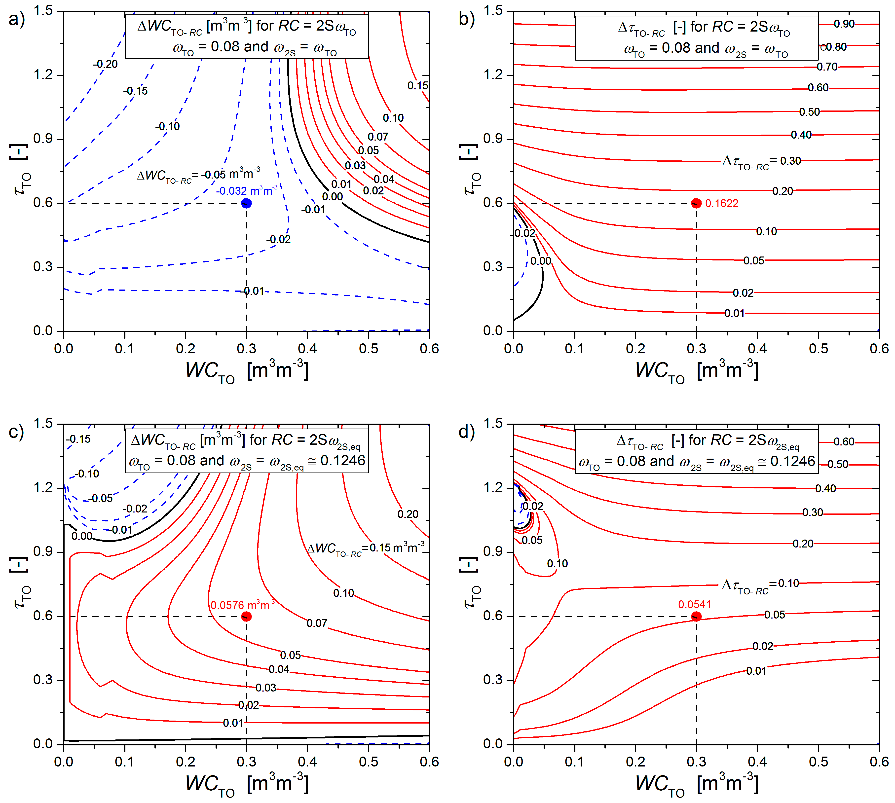
3.2. Retrievals Based on Synthetic Brightness Temperatures

After exploring differences between brightness temperatures $T_{\mathrm{B},EM}^{p,\theta }$ simulated with $EM=\left\{\mathrm{TO},1\mathrm{S},2\mathrm{S}\right\}$, this section presents differences $\mathsf{\Delta }W{C}_{\mathrm{TO}-RC}$ and $\mathsf{\Delta }{\tau }_{\mathrm{TO}-RC}$ between retrievals achieved with the “reference” Retrieval Configuration $RC={\mathrm{TO}}_{{\omega }_{\mathrm{TO}}}$ and the 2S configurations $RC=\left\{2{\mathrm{S}}_{{\omega }_{\mathrm{TO}}},2{\mathrm{S}}_{{\omega }_{2\mathrm{S},\mathrm{eq}}}\right\}$ defined in Section 2.3:

$$\begin{array}{l}\mathsf{\Delta }W{C}_{\mathrm{TO}-RC}\equiv W{C}_{\mathrm{TO}{\omega }_{\mathrm{TO}}}-W{C}_{RC}\\ \mathsf{\Delta }{\tau }_{\mathrm{TO}-RC}\equiv {\tau }_{\mathrm{TO}{\omega }_{\mathrm{TO}}}-{\tau }_{RC}\end{array}$$

(25)

Retrieval differences $\mathsf{\Delta }W{C}_{\mathrm{TO}-RC}$ and $\mathsf{\Delta }{\tau }_{\mathrm{TO}-RC}$ are intentionally based on synthetic elevation scans $T_{\mathrm{B}}^{p,{\theta }_j}=T_{\mathrm{B},\mathrm{TO}}^{p,{\theta }_j}$ simulated with the “reference” TO EM. This is because our investigation aims to quantify impacts of replacing the “reference” TO EM used in current SMOS and SMAP retrievals with 2S EM. Accordingly, retrievals $\mathbf{2}{P}_{RC}=(W{C}_{RC},{\tau }_{RC})$ are derived from synthetic elevation scans $T_{\mathrm{B}}^{p,{\theta }_j}=T_{\mathrm{B},\mathrm{TO}}^{p,{\theta }_j}$ (including ${\theta }_j=\left\{0°,5°,\dots ,60°\right\}$ and $p=\left\{\mathrm{H},\mathrm{V}\right\}$) simulated for $({\tau }_{\mathrm{TO}},{\omega }_{\mathrm{TO}},W{C}_{\mathrm{TO}})$ using the “reference” $EM=\mathrm{TO}$. Retrieval differences $\mathsf{\Delta }W{C}_{\mathrm{TO}-RC}$ and $\mathsf{\Delta }{\tau }_{\mathrm{TO}-RC}$ are computed for $0.0{\mathrm{m}}^3{\mathrm{m}}^{-3}\le W{C}_{\mathrm{TO}}\le 0.6{\mathrm{m}}^3{\mathrm{m}}^{-3}$, $0.0\le {\tau }_{\mathrm{TO}}\le 1.5$ and ${\omega }_{\mathrm{TO}}=0.08$, with further parameters used to synthesize $T_{\mathrm{B}}^{p,{\theta }_j}=T_{\mathrm{B},\mathrm{TO}}^{p,{\theta }_j}$ provided in Table 1.

Figure 5a,b show, respectively, $\mathsf{\Delta }W{C}_{\mathrm{TO}-RC}$ and $\mathsf{\Delta }{\tau }_{\mathrm{TO}-RC}$-isolines for $RC=2{\mathrm{S}}_{{\omega }_{\mathrm{TO}}}$ assuming ${\omega }_{\mathrm{TO}}={\omega }_{2\mathrm{S}}=0.08$. Figure 5c,d show corresponding $\mathsf{\Delta }W{C}_{\mathrm{TO}-RC}$ and $\mathsf{\Delta }{\tau }_{\mathrm{TO}-RC}$-isolines, respectively, for $RC=2{\mathrm{S}}_{{\omega }_{2\mathrm{S},\mathrm{eq}}}$ implying that ${\omega }_{2\mathrm{S},\mathrm{eq}}={\omega }_{2\mathrm{S},\mathrm{eq}}^{\mathrm{FM}}({\omega }_{\mathrm{TO}}=0.08)\cong 0.12458>{\omega }_{\mathrm{TO}}=0.08$ is used to compute 2S retrievals.

Figure 5 should be read the following way: Example parameter values $(W{C}_{\mathrm{TO}},{\tau }_{\mathrm{TO}})=(0.3{\mathrm{m}}^3{\mathrm{m}}^{-3},0.6)$ used to synthesize an elevation scan $T_{\mathrm{B}}^{p,{\theta }_j}=T_{\mathrm{B},\mathrm{TO}}^{p,{\theta }_j}$ with the “reference” TO EM are indicated with black dashed lines. Retrieval pairs $\mathbf{2}{P}_{RC}=(W{C}_{RC},{\tau }_{RC})$ are derived from $T_{\mathrm{B}}^{p,{\theta }_j}$. Naturally, $(W{C}_{\mathrm{TO}},{\tau }_{\mathrm{TO}})$ agree exactly with $\mathbf{2}{P}_{\mathrm{TO}{\omega }_{\mathrm{TO}}}=(W{C}_{\mathrm{TO}{\omega }_{\mathrm{TO}}},{\tau }_{\mathrm{TO}{\omega }_{\mathrm{TO}}})$ $=(0.3{\mathrm{m}}^3{\mathrm{m}}^{-3},0.6)$ retrieved with the “reference” $RC={\mathrm{TO}}_{{\omega }_{\mathrm{TO}}}$, while $\mathbf{2}{P}_{RC}=(W{C}_{RC},{\tau }_{RC})$ retrieved with $RC=\left\{2{\mathrm{S}}_{{\omega }_{\mathrm{TO}}},2{\mathrm{S}}_{{\omega }_{2\mathrm{S},\mathrm{eq}}}\right\}$ differ from $(W{C}_{\mathrm{TO}},{\tau }_{\mathrm{TO}})$. Example retrieval differences $\mathsf{\Delta }W{C}_{\mathrm{TO}-RC}$ and $\mathsf{\Delta }{\tau }_{\mathrm{TO}-RC}$ (Equation (25)) are computed for $RC=\left\{2{\mathrm{S}}_{{\omega }_{\mathrm{TO}}},2{\mathrm{S}}_{{\omega }_{2\mathrm{S},\mathrm{eq}}}\right\}$ and indicated next to the bold dots. For arbitrary parameter pairs $(W{C}_{\mathrm{TO}},{\tau }_{\mathrm{TO}})$ associated retrieval differences $\mathsf{\Delta }W{C}_{\mathrm{TO}-RC}$ and $\mathsf{\Delta }{\tau }_{\mathrm{TO}-RC}$ are represented with the labeled contour lines.

The negative difference $\mathsf{\Delta }W{C}_{\mathrm{TO}-RC}\cong -0.0324{\mathrm{m}}^3{\mathrm{m}}^{-3}$ (blue bold dot in Figure 5a) indicates the $\approx 11\%$ higher $W{C}_{RC}$ retrieved with $RC=2{\mathrm{S}}_{{\omega }_{\mathrm{TO}}}$ compared with $W{C}_{\mathrm{TO}{\omega }_{\mathrm{TO}}}=0.3{\mathrm{m}}^3{\mathrm{m}}^{-3}$ retrieved with the “reference” $RC={\mathrm{TO}}_{{\omega }_{\mathrm{TO}}}$. The positive $\mathsf{\Delta }{\tau }_{2\mathrm{S}{\omega }_{\mathrm{TO}}}\cong 0.1622$ (red bold dot in Figure 5b) represents the $\approx 28\%$ lower ${\tau }_{2\mathrm{S}{\omega }_{\mathrm{TO}}}$ compared with ${\tau }_{\mathrm{TO}{\omega }_{\mathrm{TO}}}=0.6$ retrieved with the “reference” $RC={\mathrm{TO}}_{{\omega }_{\mathrm{TO}}}$. For the same $(W{C}_{\mathrm{TO}},{\tau }_{\mathrm{TO}})=(0.3{\mathrm{m}}^3{\mathrm{m}}^{-3},0.6)$, indicated with the dashed black lines in Figure 5c,d, the positive $\mathsf{\Delta }W{C}_{2\mathrm{S}{\omega }_{2\mathrm{S},\mathrm{eq}}}\cong 0.0576{\mathrm{m}}^3{\mathrm{m}}^{-3}$ and $\mathsf{\Delta }{\tau }_{2\mathrm{S}{\omega }_{2\mathrm{S},\mathrm{eq}}}\cong 0.0541$ (red bold dots) indicate that both 2S retrievals $\mathbf{2}{P}_{RC}=(W{C}_{RC},{\tau }_{RC})$ achieved with $RC=2{\mathrm{S}}_{{\omega }_{2\mathrm{S},\mathrm{eq}}}$ are $\approx 19\%$ and $\approx 9\%$ lower than the corresponding TO retrievals $\mathbf{2}{P}_{\mathrm{TO}{\omega }_{\mathrm{TO}}}=(W{C}_{\mathrm{TO}{\omega }_{\mathrm{TO}}},{\tau }_{\mathrm{TO}{\omega }_{\mathrm{TO}}})=(0.3{\mathrm{m}}^3{\mathrm{m}}^{-3},0.6)$.

It is apparent that $\mathsf{\Delta }W{C}_{\mathrm{TO}-RC}$ and $\mathsf{\Delta }{\tau }_{\mathrm{TO}-RC}$ are significantly distinguished for $RC=2{\mathrm{S}}_{{\omega }_{\mathrm{TO}}}$. (Figure 5a,b) and $RC=2{\mathrm{S}}_{{\omega }_{2\mathrm{S},\mathrm{eq}}}$ (Figure 5c,d). Retrieval differences associated with ${\omega }_{2\mathrm{S},\mathrm{eq}}\ne {\omega }_{\mathrm{TO}}$ are at least partially compensated when considering the 2S-equivalent ${\omega }_{2\mathrm{S},\mathrm{eq}}\cong 0.1246>{\omega }_{\mathrm{TO}}=0.08$ with $RC=2{\mathrm{S}}_{{\omega }_{2\mathrm{S},\mathrm{eq}}}$. Accordingly, $\mathsf{\Delta }W{C}_{\mathrm{TO}-RC}$ and $\mathsf{\Delta }{\tau }_{\mathrm{TO}-RC}$ for $RC=2{\mathrm{S}}_{{\omega }_{2\mathrm{S},\mathrm{eq}}}$ (Figure 5c,d) represent impacts of multiple scattering and multiple reflections neglected in TO EM more exclusively than the $\mathsf{\Delta }W{C}_{\mathrm{TO}-RC}$ and $\mathsf{\Delta }{\tau }_{\mathrm{TO}-RC}$ for $RC=2{\mathrm{S}}_{{\omega }_{\mathrm{TO}}}$ (Figure 5a,b).

Comparison between $\mathsf{\Delta }W{C}_{\mathrm{TO}-RC}$ computed for $RC=2{\mathrm{S}}_{{\omega }_{\mathrm{TO}}}$ and $RC=2{\mathrm{S}}_{{\omega }_{2\mathrm{S},\mathrm{eq}}}$ illustrates the following picture: For $RC=2{\mathrm{S}}_{{\omega }_{\mathrm{TO}}}$ the $\mathsf{\Delta }W{C}_{\mathrm{TO}-RC}$ (Figure 5a) are mostly negative (blue dashed contours) except for $W{C}_{\mathrm{TO}}\gtrsim 0.40{\mathrm{m}}^3{\mathrm{m}}^{-3}$ and ${\tau }_{\mathrm{TO}}\gtrsim 0.4$. On the other hand, the $\mathsf{\Delta }W{C}_{\mathrm{TO}-RC}$ computed for $RC=2{\mathrm{S}}_{{\omega }_{2\mathrm{S},\mathrm{eq}}}$ (Figure 5c) are mostly positive (red solid contour lines) except for $W{C}_{\mathrm{TO}}\lesssim 0.25{\mathrm{m}}^3{\mathrm{m}}^{-3}$ and ${\tau }_{\mathrm{TO}}\gtrsim 0.9$. This implies for rather dry soils under dense vegetation, $W{C}_{RC}$-retrievals using $RC=2{\mathrm{S}}_{{\omega }_{2\mathrm{S},\mathrm{eq}}}$ are expected to be smaller than “reference” retrievals $W{C}_{\mathrm{TO}{\omega }_{\mathrm{TO}}}$. Generally, $\mathsf{\Delta }W{C}_{\mathrm{TO}-RC}$ increases with increasing optical depth and soil water content, but remains $\lesssim 0.05{\mathrm{m}}^3{\mathrm{m}}^{-3}$ for moderately wet soils ($\lesssim 0.30{\mathrm{m}}^3{\mathrm{m}}^{-3}$) under vegetation cover with optical depth $\lesssim 0.6$. Furthermore, $\mathsf{\Delta }W{C}_{\mathrm{TO}-RC}$ shown in Figure 5c suggests that over vegetated areas with vastly differing optical depth, 2S retrievals $W{C}_{RC}$ achieved with $RC=2{\mathrm{S}}_{{\omega }_{2\mathrm{S},\mathrm{eq}}}$ may exhibit an increased dynamic range compared to $W{C}_{\mathrm{TO}{\omega }_{\mathrm{TO}}}$ achieved with “reference” $RC={\mathrm{TO}}_{{\omega }_{\mathrm{TO}}}$.

Due to the consideration of ${\omega }_{2\mathrm{S},\mathrm{eq}}\cong 0.1246>{\omega }_{\mathrm{TO}}=0.08$ in $C=2{\mathrm{S}}_{{\omega }_{2\mathrm{S},\mathrm{eq}}}$, resulting $\mathsf{\Delta }{\tau }_{\mathrm{TO}-RC}$ values (Figure 5d) are generally smaller than the ones achieved with $RC=2{\mathrm{S}}_{{\omega }_{\mathrm{TO}}}$ (Figure 5b). However, for $RC=2{\mathrm{S}}_{{\omega }_{\mathrm{TO}}}$ and $RC=2{\mathrm{S}}_{{\omega }_{2\mathrm{S},\mathrm{eq}}}$, $\mathsf{\Delta }{\tau }_{\mathrm{TO}-RC}$ is almost exclusively positive (red solid contour lines) implying that 2S retrievals of optical depth are expected to be smaller than ${\tau }_{\mathrm{TO}{\omega }_{\mathrm{TO}}}$ retrieved with the “reference” $RC={\mathrm{TO}}_{{\omega }_{\mathrm{TO}}}$. This model-based finding will be confirmed experimentally in the subsequent section. Again, ${\tau }_{\mathrm{TO}{\omega }_{\mathrm{TO}}}>{\tau }_{RC}$ ($RC=\left\{2{\mathrm{S}}_{{\omega }_{\mathrm{TO}}},2{\mathrm{S}}_{{\omega }_{2\mathrm{S},\mathrm{eq}}}\right\}$) is due to the TO EM’s inadequate representation of microwave emission of soil covered with optically thick and scattering vegetation, which leads to misinterpretation of increased optical depth.

3.3. Retrievals Based on Brightness Temperatures Measured over a Deciduous Forest

Figure 6a,b show the same auxiliary in-situ data (soil temperatures $T_{\mathrm{s}}$ (magenta squares), 12-h averages of precipitation $P$ (blue columns), Relative Foliation $RF$ (green line), forest soil Water Content $W{C}_{\mathrm{in}-\mathrm{situ}}$ $~5\mathrm{cm}$ below the litter layer (black stars)) as shown in Figure 3a,b. Figure 6c,d show, respectively, time series of forest soil Water Content $W{C}_{RC}$ and canopy optical depth ${\tau }_{RC}$ retrieved from the measured elevation scans $T_{\mathrm{B}}^{p,{\theta }_j}$ ($p=\left\{\mathrm{H},\mathrm{V}\right\}$, ${\theta }_j=\left\{46°,50°,54°,58°\right\}$) shown in Figure 3c,d. The retrieval approach outlined in Section 2.3 is used with the “reference” TO Retrieval Configuration $RC={\mathrm{TO}}_{{\omega }_{\mathrm{TO}}}$ and the 2S configurations $RC=\left\{2{\mathrm{S}}_{{\omega }_{\mathrm{TO}}},2{\mathrm{S}}_{{\omega }_{2\mathrm{S},\mathrm{eq}}}\right\}$. Auxiliary parameter values are provided in Table 1. Retrievals $\mathbf{2}{P}_{RC}=(W{C}_{RC},{\tau }_{RC})$ achieved with $RC={\mathrm{TO}}_{{\omega }_{\mathrm{TO}}}$, assuming ${\omega }_{\mathrm{TO}}=0.08$, are indicated with black squares; retrievals achieved with $RC=2{\mathrm{S}}_{{\omega }_{\mathrm{TO}}}$, assuming ${\omega }_{2\mathrm{S}}={\omega }_{\mathrm{TO}}=0.08$, are shown with green circles; and retrievals achieved with $RC=2{\mathrm{S}}_{{\omega }_{2\mathrm{S},\mathrm{eq}}}$, considering ${\omega }_{2\mathrm{S},\mathrm{eq}}={\omega }_{2\mathrm{S},\mathrm{eq}}^{\mathrm{FM}}({\omega }_{\mathrm{TO}}=0.08)\cong 0.1246$, are shown with red circles.

Responses of $W{C}_{RC}$ (Figure 6c) with respect to $W{C}_{\mathrm{in}-\mathrm{situ}}$ (Figure 6b) are noticeable during the two strongest precipitation periods (Figure 6a) taking place at around the 1st and the 29th of July 2005. This finding corroborates with the response of $T_{\mathrm{B}}^{p,{\theta }_j}$ to $W{C}_{\mathrm{in}-\mathrm{situ}}$ discussed in Section 2.5. However, these increases of $W{C}_{RC}$ show that the drops of $T_{\mathrm{B}}^{p,{\theta }_j}$ (Figure 3) are not primarily the result of lowered soil temperature due to rain. Changes in forest soil water content are recognized in retrieved $W{C}_{RC}$, in the presence of understory, leaf litter, and forest canopy, which is semi-transparent at L-band as demonstrated in [5,6]. The latter theoretical finding is consistent with our earlier experimental observation outlined in [7,8], and corroborated by the values of retrieved canopy optical depth (Figure 6d). Figure 6c shows that $W{C}_{RC}$ retrieved with $RC=2{\mathrm{S}}_{{\omega }_{\mathrm{TO}}}$ is unrealistically higher than $W{C}_{RC}$ achieved with the other two configurations $RC=\left\{{\mathrm{TO}}_{{\omega }_{\mathrm{TO}}},2{\mathrm{S}}_{{\omega }_{2\mathrm{S},\mathrm{eq}}}\right\}$, which both agree reasonably well with $W{C}_{\mathrm{in}-\mathrm{situ}}$ (Figure 6b). This demonstrates the necessity to consider ${\omega }_{2\mathrm{S},\mathrm{eq}}\cong 0.1246>{\omega }_{\mathrm{TO}}=0.08$ with $RC=2{\mathrm{S}}_{{\omega }_{2\mathrm{S},\mathrm{eq}}}$ instead of ${\omega }_{2\mathrm{S}}={\omega }_{\mathrm{TO}}=0.08$ considered with $RC=2{\mathrm{S}}_{{\omega }_{\mathrm{TO}}}$. Furthermore, from Figure 6d the relative magnitudes ${\tau }_{\mathrm{TO}{\omega }_{\mathrm{TO}}}>{\tau }_{2\mathrm{S}{\omega }_{2\mathrm{S},\mathrm{eq}}}>{\tau }_{2\mathrm{S}{\omega }_{\mathrm{TO}}}$ are consistent with the corresponding retrievals derived from synthetic $T_{\mathrm{B}}^{p,{\theta }_j}$ (Figure 5b,d). It is likely that ${\tau }_{RC}$ retrieved with the “reference” $RC={\mathrm{TO}}_{{\omega }_{\mathrm{TO}}}$ tends to be over-estimated for reasons discussed earlier. This misleads TO EM to compensate by increasing vegetation emission.

Table 2. Vegetation optical depths $\langle {\tau }_{RC}\rangle \pm \mathsf{\Delta }{\tau }_{RC}$ and relative variability $\mathsf{\sigma }{\tau }_{RC}=\mathsf{\Delta }{\tau }_{RC}/\langle {\tau }_{RC}\rangle$ retrieved with the “reference” $RC={\mathrm{TO}}_{{\omega }_{\mathrm{TO}}}$ and 2S retrieval configurations $RC=\left\{2{\mathrm{S}}_{{\omega }_{\mathrm{TO}}},2{\mathrm{S}}_{{\omega }_{2\mathrm{S},\mathrm{eq}}}\right\}$ during the foliage-free and the fully foliated forest canopy.

RC	$\langle {\mathit{\tau }}_{\mathit{R}\mathit{C}}\rangle \pm \mathsf{\Delta }{\mathit{\tau }}_{\mathit{R}\mathit{C}}$$\mathbf{and}\mathsf{\sigma }{\mathit{\tau }}_{\mathit{R}\mathit{C}}[\%]$
	$\mathbf{T}{\mathbf{O}}_{{\mathit{\omega }}_{\mathbf{T}\mathbf{O}}}$	$2{\mathbf{S}}_{{\mathit{\omega }}_{\mathbf{T}\mathbf{O}}}$	$2{\mathbf{S}}_{{\mathit{\omega }}_{2\mathbf{S},\mathbf{e}\mathbf{q}}}$
foliage-free	0.6756 ± 0.1116 16.5%	0.5051 ± 0.0540 10.7%	0.5754 ± 0.0726 12.6%
fully foliated	0.7113 ± 0.0875 12.3%	0.5808 ± 0.0489 8.4%	0.6229 ± 0.0694 11.1%

provides mean ${\tau }_{RC}$, standard deviation $\mathsf{\Delta }{\tau }_{RC}$, and relative variability $\mathsf{\sigma }{\tau }_{RC}=\mathsf{\Delta }{\tau }_{RC}/{\tau }_{RC}$ of optical depth retrieved for the foliage-free periods (1st of March 2005–14th of April 2005 and 12th of December 2005–7th of January 2006) and the fully foliated period (1st of June 2005–26th of October 2005). Means ${\tau }_{RC}$ of the foliage-free forest canopy are smaller than ${\tau }_{RC}$ of the fully foliated canopy for all $RC=\left\{{\mathrm{TO}}_{{\omega }_{\mathrm{TO}}},2{\mathrm{S}}_{{\omega }_{\mathrm{TO}}},2{\mathrm{S}}_{{\omega }_{2\mathrm{S},\mathrm{eq}}}\right\}$. It is known from theoretical investigations [5,6] that leaves play a minor role in the propagation of thermal microwaves at L-band. However, it is likely that for the foliated period Vegetation Water Content (VWC) is higher than for foliage-free periods, suggesting that optical depth is also higher for the foliated than for the foliage-free forest. Accordingly, increased ${\tau }_{RC}$ retrieved for the foliated period is meaningful. Furthermore, $\mathsf{\sigma }{\tau }_{RC}$ retrieved with $RC=\left\{2{\mathrm{S}}_{{\omega }_{\mathrm{TO}}},2{\mathrm{S}}_{{\omega }_{2\mathrm{S},\mathrm{eq}}}\right\}$ is smaller than $\mathsf{\sigma }{\tau }_{RC}$ achieved with $RC={\mathrm{TO}}_{{\omega }_{\mathrm{TO}}}$. This suggests that forest optical depth retrieved with 2S configurations are less noisy than corresponding retrievals achieved with the “reference” TO configuration $RC={\mathrm{TO}}_{{\omega }_{\mathrm{TO}}}$.

Further insight into the time series of retrievals is provided in Figure 7. Scatter plots of $\mathbf{2}{P}_{RC}=(W{C}_{RC},{\tau }_{RC})$ achieved for $RC={\mathrm{TO}}_{{\omega }_{\mathrm{TO}}}$ (black squares), $RC=2{\mathrm{S}}_{{\omega }_{\mathrm{TO}}}$ (green open circles), and $RC=2{\mathrm{S}}_{{\omega }_{2\mathrm{S},\mathrm{eq}}}$ (red open circles) are shown in Figure 7a. Probabilities of $W{C}_{RC}$ and ${\tau }_{RC}$ are depicted with the histograms in Figure 7b,c, with respective statistical parameters (mean $\langle \dots \rangle$ and standard deviation $\mathsf{\Delta }\dots$) in the upper right of Figure 7.

As discussed in connection with Figure 6c, $W{C}_{RC}$ retrieved with $RC=2{\mathrm{S}}_{{\omega }_{\mathrm{TO}}}$ (green histogram in Figure 7b) is systematically higher than $W{C}_{RC}$ retrieved with the “reference” $RC={\mathrm{TO}}_{{\omega }_{\mathrm{TO}}}$ (black histogram in Figure 7b) and unrealistically higher than in-situ $W{C}_{\mathrm{in}-\mathrm{situ}}$ (Figure 6b). The use of the 2S-equivalent ${\omega }_{2\mathrm{S},\mathrm{eq}}=0.1246>{\omega }_{\mathrm{TO}}=0.08$ with $RC=2{\mathrm{S}}_{{\omega }_{2\mathrm{S},\mathrm{eq}}}$ yields $W{C}_{RC}$ (red histogram in Figure 7b) similar to those retrieved with $RC={\mathrm{TO}}_{{\omega }_{\mathrm{TO}}}$ and $W{C}_{\mathrm{in}-\mathrm{situ}}$. This demonstrates the necessity of using the constant 2S-equivalent ${\omega }_{2\mathrm{S},\mathrm{eq}}>{\omega }_{\mathrm{TO}}$ with the 2S retrieval configuration, and the adequacy of the respective transformation ${\omega }_{\mathrm{TO}}=0.08\mapsto {\omega }_{2\mathrm{S},\mathrm{eq}}=0.1246$ computed with the Fast Model (FM) (Equation (23)).

Likewise, the already recognized relative magnitudes of the retrievals ${\tau }_{\mathrm{TO}{\omega }_{\mathrm{TO}}}>{\tau }_{2\mathrm{S}{\omega }_{2\mathrm{S},\mathrm{eq}}}>{\tau }_{2\mathrm{S}{\omega }_{\mathrm{TO}}}$ are obvious from the respective histograms shown in Figure 7c and quantified by the associated mean values ${\tau }_{RC}$. Beyond that, seasonal variabilities $\mathsf{\Delta }{\tau }_{RC}\lesssim 0.089$ of the 2S retrievals ${\tau }_{RC}$ ($RC=\left\{2{\mathrm{S}}_{{\omega }_{\mathrm{TO}}},2{\mathrm{S}}_{{\mathsf{\omega }}_{2\mathrm{S},\mathrm{eq}}}\right\}$) are smaller than $\mathsf{\Delta }{\tau }_{RC}\cong 0.116$ of ${\tau }_{RC}$ retrieved with the “reference” $RC={\mathrm{TO}}_{{\omega }_{\mathrm{TO}}}$. The scatter $\mathsf{\Delta }{\tau }_{\mathrm{TO}{\omega }_{\mathrm{TO}}}\cong 0.116$ seems too high considering the small seasonal change expected for the forest optical depth mainly due to increased VWC during the growing season compared to the winter season. In this regard, $\mathsf{\Delta }{\tau }_{RC}\lesssim 0.089$ associated with the 2S configurations is more realistic and indicates another advantage of 2S EM over TO EM in application to the retrieval of optical depth of dense and scattering vegetation.

4. Summary and Conclusions

The goal of this study is the demonstration of benefits of using the Two-Stream (2S) Emission Model (EM) instead of the “Tau Omega” (TO) EM to achieve Two-Parameter (2P) retrievals $\mathbf{2}{P}_{RC}=(W{C}_{RC},{\tau }_{RC})$ of soil liquid Water Content and optical depth from elevation scans of L-band brightness temperatures $T_{\mathrm{B}}^{p,{\theta }_j}$ over areas covered with dense and scattering vegetation. This goal is achieved by first analyzing the differences between brightness temperatures $T_{\mathrm{B},EM}^{p,\theta }$ simulated with the “reference” TO EM, the One-Stream (1S) EM, and 2S EM (Section 3.1). These EMs converge for sparse vegetation, but for scattering albedos and optical depth typical of forests, differences between $T_{\mathrm{B},EM}^{p,\theta }$ simulated with $EM=\left\{\mathrm{TO},1\mathrm{S},2\mathrm{S}\right\}$ are several Kelvins and exceed the instrumental noise of SMOS and SMAP. Thus, it is expected that retrievals are noticeably impacted when using 2S EM as a replacement for the “reference” TO EM implemented in current operational SMOS and SMAP retrieval algorithms.

The single layer $EM=\left\{\mathrm{TO},1\mathrm{S},2\mathrm{S}\right\}$ (Figure 1) are outlined in Section 2.1 and Section 2.2. The EM-specific assumptions made in the simplification of the radiative transfer equation and the resulting representation of $T_{\mathrm{B},EM}^{p,\theta }$ are outlined. The “reference” TO EM is the least sophisticated approach representing $T_{\mathrm{B},\mathrm{TO}}^{p,\theta }$ as the sum of radiance: (i) emitted by the soil surface and attenuated by the vegetation, (ii) upwelling vegetation emission, and (iii) downwelling emission of vegetation reflected by the soil surface and attenuated by the vegetation. In TO EM scattering is considered as a loss mechanism only, and thus, it leads to an underestimation of emitted radiation. It does not take into account multiple reflections between vegetation and the soil surface, and it is inconsistent with Kirchhoff’s law. Similar to TO EM, 1S EM is also a 0^th-order solution of the radiative transfer equation. However, 1S EM is an improved version of TO EM, taking into account multiple reflections between vegetation and the soil surface, and it is consistent with Kirchhoff’s law. 2S EM is a 1^st-order solution of the radiative transfer equation, and it is the most advanced EM investigated here to simulate $T_{\mathrm{B},2\mathrm{S}}^{p,\theta }$. 2S EM considers multiple scattering in vegetation, multiple reflections between vegetation and the soil surface, and it is consistent with Kirchhoff’s law. Furthermore, the formulation of the single layer 2S EM is as simple as TO EM. Technically speaking, this implies that 2S EM is at least as suitable as TO EM for implementation in a retrieval algorithm based on the minimization of differences between measured and simulated brightness temperatures.

Ultimately, we analyze retrievals $\mathbf{2}{P}_{RC}=(W{C}_{RC},{\tau }_{RC})$ considering the TO Retrieval Configuration $RC={\mathrm{TO}}_{{\omega }_{\mathrm{TO}}}$ and the 2S configurations $RC=\left\{2{\mathrm{S}}_{{\omega }_{\mathrm{TO}}},2{\mathrm{S}}_{{\omega }_{2\mathrm{S},\mathrm{eq}}}\right\}$ explained in Section 2.3. Configuration $RC={\mathrm{TO}}_{{\omega }_{\mathrm{TO}}}$. is considered as the “reference” because it employs the “reference” TO EM, with the respective constant vegetation scattering albedo ${\omega }_{\mathrm{TO}}$, as implemented in current SMOS retrievals. The 2S configurations $RC=\left\{2{\mathrm{S}}_{{\omega }_{\mathrm{TO}}},2{\mathrm{S}}_{{\omega }_{2\mathrm{S},\mathrm{eq}}}\right\}$ use 2S EM and assume the respective scattering albedos ${\omega }_{2\mathrm{S}}={\omega }_{\mathrm{TO}}$ and ${\omega }_{2\mathrm{S},\mathrm{eq}}>{\omega }_{\mathrm{TO}}$ as constants. Perceptions of ${\omega }_{EM}$ are different for $EM=\mathrm{TO}$ and $EM=2\mathrm{S}$. Accordingly, a Fast Model (FM) (Equation (23)) is developed to transform ${\omega }_{\mathrm{TO}}\mapsto {\omega }_{2\mathrm{S},\mathrm{eq}}={\omega }_{2\mathrm{S},\mathrm{eq}}^{\mathrm{FM}}({\omega }_{\mathrm{TO}})$ (Figure 2) in order to compare $\mathbf{2}{P}_{RC}=(W{C}_{RC},{\tau }_{RC})$ achieved with TO and 2S configurations on a fair basis.

Differences $\mathsf{\Delta }W{C}_{\mathrm{TO}-RC}$ and $\mathsf{\Delta }{\tau }_{\mathrm{TO}-RC}$ between synthetic retrievals $\mathbf{2}{P}_{RC}=(W{C}_{RC},{\tau }_{RC})$ achieved with “reference” $RC={\mathrm{TO}}_{{\omega }_{\mathrm{TO}}}$ and the 2S configurations $RC=\left\{2{\mathrm{S}}_{{\omega }_{\mathrm{TO}}},2{\mathrm{S}}_{{\omega }_{2\mathrm{S},\mathrm{eq}}}\right\}$ are presented in Section 3.2. Retrievals underlying elevation scans $T_{\mathrm{B}}^{p,{\theta }_j}=T_{\mathrm{B},\mathrm{TO}}^{p,{\theta }_j}$ are simulated with the “reference” TO EM. It is shown that retrieval differences are diminished when using ${\omega }_{2\mathrm{S},\mathrm{eq}}\cong 0.1246>{\omega }_{\mathrm{TO}}=0.08$ with $RC=2{\mathrm{S}}_{{\omega }_{2\mathrm{S},\mathrm{eq}}}$ instead of using ${\omega }_{2\mathrm{S}}={\omega }_{\mathrm{TO}}=0.08$ with $RC=2{\mathrm{S}}_{{\omega }_{\mathrm{TO}}}$. This demonstrates that the approach developed to transform ${\omega }_{\mathrm{TO}}\mapsto {\omega }_{2\mathrm{S},\mathrm{eq}}$ (Section 2.4) is adequate. The analysis of retrieval differences $\mathsf{\Delta }W{C}_{\mathrm{TO}-RC}$ (Figure 5a,c) indicates that $W{C}_{RC}$ achieved with $RC=2{\mathrm{S}}_{{\omega }_{2\mathrm{S},\mathrm{eq}}}$ are smaller than $W{C}_{RC}$ achieved with $RC={\mathrm{TO}}_{{\omega }_{\mathrm{TO}}}$, except for rather dry soils ($W{C}_{\mathrm{TO}}\lesssim 0.25{\mathrm{m}}^3{\mathrm{m}}^{-3}$) under very dense vegetation (${\tau }_{\mathrm{TO}}\gtrsim 0.9$). However, apart from this, $\mathsf{\Delta }W{C}_{\mathrm{TO}-RC}$ ($RC=2{\mathrm{S}}_{{\omega }_{2\mathrm{S},\mathrm{eq}}}$) is increasingly positive with increasing soil water content and vegetation optical depth. Optical depths ${\tau }_{RC}$ retrieved with $RC=2{\mathrm{S}}_{{\omega }_{2\mathrm{S},\mathrm{eq}}}$ are generally smaller than ${\tau }_{RC}$ retrieved with $RC={\mathrm{TO}}_{{\omega }_{\mathrm{TO}}}$ due to inappropriate modelling of $T_{\mathrm{B},\mathrm{TO}}^{p,\theta }$ in the presence of dense and scattering vegetation. Resulting positive retrieval differences $\mathsf{\Delta }{\tau }_{\mathrm{TO}-RC}$ are noticeable and increase with increasing optical depth (Figure 5b,d). This theoretical finding suggests that TO retrievals ${\tau }_{RC}$ ($RC={\mathrm{TO}}_{{\omega }_{\mathrm{TO}}}$, ${\omega }_{\mathrm{TO}}=0.08$) performed over dense forests are expected to exaggerate the reality due to incorrect interpretation of scattering and neglecting multiple reflections. It is concluded that optical depth of forests should be estimated with a retrieval approach that employs 2S EM rather than TO EM.

Comparative retrievals $\mathbf{2}{P}_{RC}=(W{C}_{RC},{\tau }_{RC})$. achieved with $RC={\mathrm{TO}}_{{\omega }_{\mathrm{TO}}}$ and $RC=\left\{2{\mathrm{S}}_{{\omega }_{\mathrm{TO}}},2{\mathrm{S}}_{{\omega }_{2\mathrm{S},\mathrm{eq}}}\right\}$ based on experimental elevations scans $T_{\mathrm{B}}^{p,{\theta }_j}$ (Figure 3c,d) measured from a tower located in a deciduous forest are presented in Section 3.3. It is shown that the seasonal mean $\langle W{C}_{RC}\rangle =0.6939 {\mathrm{m}}^3{\mathrm{m}}^{-3}$ retrieved with $RC=2{\mathrm{S}}_{{\omega }_{\mathrm{TO}}}$ largely overestimate in-situ $\langle W{C}_{\mathrm{in}-\mathrm{situ}}\rangle =0.3066 {\mathrm{m}}^3{\mathrm{m}}^{-3}$. In contrast, $\langle W{C}_{RC}\rangle =0.2515{\mathrm{m}}^3{\mathrm{m}}^{-3}$ retrieved with $RC={\mathrm{TO}}_{{\omega }_{\mathrm{TO}}}$ and $\langle W{C}_{RC}\rangle =0.2364 {\mathrm{m}}^3{\mathrm{m}}^{-3}$ retrieved with $RC=2{\mathrm{S}}_{{\omega }_{2\mathrm{S},\mathrm{eq}}}$ are in reasonable agreement with $W{C}_{\mathrm{in}-\mathrm{situ}}$ (Figure 6b,c and Figure 7a,b). Furthermore, the fact that $\langle W{C}_{RC}\rangle$ retrieved with $RC=2{\mathrm{S}}_{{\omega }_{2\mathrm{S},\mathrm{eq}}}$ is slightly smaller than $\langle W{C}_{RC}\rangle$ retrieved with the “reference” $RC={\mathrm{TO}}_{{\omega }_{\mathrm{TO}}}$ ($~6\%$) is consistent with the finding from the synthetic retrieval analyses (Section 3.2).

The comparison between $W{C}_{\mathrm{in}-\mathrm{situ}}$ (measured $~5\mathrm{cm}$ below the litter) and retrieved $W{C}_{RC}$ revealed contemporaneous responses for the two strongest precipitation periods (1st and 29th of July 2005). This proves experimentally that changes in forest soil water content can be detected with L-band radiometry, even in presence of leaf litter and understory. Nevertheless, it is argued (Section 2.5) that quantitative forest soil water content retrievals can be hindered by leaf litter due to its significant impact on microwave emission, and the fact that litter and soil water contents are hydrologically decoupled in many cases.

In spite of the recognized small impact of using either $RC={\mathrm{TO}}_{{\omega }_{\mathrm{TO}}}$ or $RC=2{\mathrm{S}}_{{\omega }_{2\mathrm{S},\mathrm{eq}}}$ on $W{C}_{RC}$ retrieved from the tower-based observations $T_{\mathrm{B}}^{p,{\theta }_j}$, retrievals of soil water content derived from large-scale spaceborne $T_{\mathrm{B}}^{p,{\theta }_j}$ (≈40 km × 40 km in case of SMOS) can be noticeably affected by the choice of the EM implemented in the retrieval algorithm. Especially, this is expected for pixels with significant areal forest fractions. With increasing forest fraction, simulation of SMOS-measured brightness temperatures becomes increasingly dependent on the EM, causing retrieved $W{C}_{RC}$ to be sensitive to the choice of the EM.

Seasonal means $\langle {\tau }_{RC}\rangle =0.6891$ achieved with $RC={\mathrm{TO}}_{{\omega }_{\mathrm{TO}}}$ are $~13\%$ higher than $\langle {\tau }_{RC}\rangle =0.5949$ achieved with $RC=2{\mathrm{S}}_{{\omega }_{2\mathrm{S},\mathrm{eq}}}$, and even $~21\%$ higher than $\langle {\tau }_{RC}\rangle =0.5391$ achieved with $RC=2{\mathrm{S}}_{{\omega }_{\mathrm{TO}}}$ (upper right of Figure 7). This experimental finding is consistent with the synthetic retrieval analysis (Section 3.2). It emphasizes that ${\tau }_{RC}$ of forests retrieved with $RC={\mathrm{TO}}_{{\omega }_{\mathrm{TO}}}$ overestimate the reality due its inadequate representation of $T_{\mathrm{B},\mathrm{TO}}^{p,\theta }$ of forests. However, all of the investigated $RC=\left\{{\mathrm{TO}}_{{\omega }_{\mathrm{TO}}},2{\mathrm{S}}_{{\omega }_{\mathrm{TO}}},2{\mathrm{S}}_{{\omega }_{2\mathrm{S},\mathrm{eq}}}\right\}$ revealed higher means $\langle {\tau }_{RC}\rangle$ for the foliated forest than for the foliage-free canopy (Table 2). This experimental finding demonstrates the potential of L-band radiometry to observe phenological changes of a forest canopy.

A further advantage of 2S EM over the “reference” TO EM, used for current operational SMOS and SMAP retrievals, is its wider applicability range. For instance, the “soft layer” assumption (neglecting reflection and refraction at the upper bound of the layer atop the ground) is not necessary with 2S EM, while it is inherent to TO EM (Section 2.1 and Section 2.2). As an example, consideration of a “refractive layer”, as is possible with the 2S EM, is necessary to retrieve snow density and ground permittivity from L-band radiometry. Generally, unification of retrieval algorithms using a consistent EM allows for different applications (e.g., soil water content and optical depth or snow states and soil permittivity), and corresponding assumptions (“soft layer” or “refractive layer”). Accordingly, implementing 2S EM in SMOS and SMAP retrieval algorithms as a replacement of TO EM is seen at least as a conceptual improvement.

References

- Nemani, R.R.; Keeling, C.D.; Hashimoto, H.; Jolly, W.M.; Piper, S.C.; Tucker, C.J.; Myneni, R.B.; Running, S.W. Climate-driven increases in global terrestrial net primary production from 1982 to 1999. Science 2003, 300, 1560–1563. [Google Scholar] [CrossRef] [PubMed]
- Schmugge, T. Remote sensing of soil moisture. In Encyclopedia of Hydrological Forecasting; Anderson, M.G., Burt, T., Eds.; John Wiley & Sons: Chichester, UK, 1985; pp. 101–124. [Google Scholar]
- Shutko, A.M. Microwave radiometry of lands under natural and artificial moistening. IEEE Trans. Geosci. Remote Sens. 1982, GE-20, 18–26. [Google Scholar] [CrossRef]
- Mätzler, C. Thermal Microwave Radiation: Applications for Remote Sensing; IEE Electromagnetic Waves Series No. 52; Institution of Engineering and Technology: London, UK, 2006; Volume 52. [Google Scholar]
- Ferrazzoli, P.; Guerriero, L. Passive microwave remote sensing of forests: A model investigation. IEEE Trans. Geosci. Remote Sens. 1996, 34, 433–443. [Google Scholar] [CrossRef]
- Ferrazzoli, P.; Guerriero, L.; Wigneron, J.-P. Simulating L-band emission of forests in view of future satellite applications. IEEE Trans. Geosci. Remote Sens. 2002, 40, 2700–2708. [Google Scholar] [CrossRef]
- Guglielmetti, M.; Schwank, M.; Mätzler, C.; Oberdörster, C.; Vanderborght, J.; Flühler, H. Measured microwave radiative transfer properties of a deciduous forest canopy. Remote Sens. Environ. 2007, 523–532. [Google Scholar] [CrossRef]
- Guglielmetti, M.; Schwank, M.; Mätzler, C.; Oberdörster, C.; Vanderborght, J.; Flühler, H. Fosmex: Forest soil moisture experiments with microwave radiometry. IEEE Trans. Geosci. Remote Sens. 2008, 46, 727–735. [Google Scholar] [CrossRef]
- Ulaby, F.T.; Razani, M.; Dobson, M.C. Effects of vegetation cover on the microwave radiometric sensitivity to soil moisture. IEEE Trans. Geosci. Remote Sens. 1983, GE-21, 51–61. [Google Scholar] [CrossRef]
- Grant, J.P.; Wigneron, J.P.; De Jeu, R.A.M.; Lawrence, H.; Mialon, A.; Richaume, P.; Al Bitar, A.; Drusch, M.; van Marle, M.J.E.; Kerr, Y. Comparison of SMOS and AMSR-E vegetation optical depth to four MODIS-based vegetation indices. Remote Sens. Environ. 2016, 172, 87–100. [Google Scholar] [CrossRef]
- Van de Griend, A.A.; Wigneron, J.-P. The B-factor as a function of frequency and canopy type at H-polarization. IEEE Trans. Geosci. Remote Sens. 2004, 42, 786–794. [Google Scholar] [CrossRef]
- Kerr, Y.H.; Waldteufel, P.; Wigneron, J.; Martinuzzi, J.; Font, J.; Berger, M. Soil moisture retrieval from space: The soil moisture and ocean salinity (SMOS) mission. IEEE Trans. Geosci. Remote Sens. 2001, 39, 1729–1735. [Google Scholar] [CrossRef]
- Lagerloef, G.; Colomb, F.R.; Le Vine, D.; Wentz, F.; Yueh, S.; Ruf, C.; Lilly, J.; Gunn, J.; Chao, Y.I.; Decharon, A.; et al. The AQUARIUS/SAC-D mission designed to meet the salinity remote-sensing challenge. Oceanography 2008, 21, 68–81. [Google Scholar] [CrossRef]
- Vine, D.M.L.; Lagerloef, G.S.E.; Torrusio, S.E. Aquarius and remote sensing of sea surface salinity from space. Proc. IEEE 2010, 98, 688–703. [Google Scholar] [CrossRef]
- Bindlish, R.; Jackson, T.; Cosh, M.; Zhao, T.; Neill, P.O. Global soil moisture from the aquarius/sac-d satellite: Description and initial assessment. IEEE Geosci Remote Sens. 2015, 12, 923–927. [Google Scholar] [CrossRef]
- Kerr, Y.H.; Waldteufel, P.; Wigneron, J.P.; Delwart, S.; Cabot, F.; Boutin, J.; Escorihuela, M.J.; Font, J.; Reul, N.; Gruhier, C.; et al. The SMOS mission: New tool for monitoring key elements of the global water cycle. Proc. IEEE 2010, 98, 666–687. [Google Scholar] [CrossRef] [Green Version]
- Entekhabi, D.; Njoku, E.G.; O’Neill, P.E.; Kellogg, K.H.; Crow, W.T.; Edelstein, W.N.; Entin, J.K.; Goodman, S.D.; Jackson, T.J.; Johnson, J.; et al. The Soil Moisture Active Passive (SMAP) Mission. Proc. IEEE 2010, 98, 704–716. [Google Scholar] [CrossRef]
- McMullan, K.; Brown, M.A.; Martín-Neira, M.; Rits, W.; Ekholm, S.; Marti, J.; Lemanczyk, J. SMOS: The payload. IEEE Trans. Geosci. Remote Sens. 2008, 46, 594–605. [Google Scholar] [CrossRef]
- Lemmetyinen, J.; Schwank, M.; Rautiainen, K.; Kontu, A.; Parkkinen, T.; Mätzler, C.; Wiesmann, A.; Wegmüller, U.; Derksen, C.; Toose, P.; et al. Snow density and ground permittivity retrieved from L-band radiometry: Application to experimental data. Remote Sens. Environ. 2016, 180, 377–391. [Google Scholar] [CrossRef]
- Naderpour, R.; Schwank, M. Snow wetness retrieved from L-band radiometry. Remote Sens. 2018, 10, 359. [Google Scholar] [CrossRef]
- Naderpour, R.; Schwank, M.; Mätzler, C. Davos-laret remote sensing field laboratory: 2016/2017 winter season L-band measurements data-processing and analysis. Remote Sens. 2017, 9, 1185. [Google Scholar] [CrossRef]
- Naderpour, R.; Schwank, M.; Mätzler, C.; Lemmetyinen, J.; Steffen, K. Snow density and ground permittivity retrieved from L-band radiometry: A retrieval sensitivity analysis. IEEE J. Sel. Top. Appl. Earth Obs. Remote Sens. 2017, 10, 3148–3161. [Google Scholar] [CrossRef]
- Schwank, M.; Mätzler, C.; Wiesmann, A.; Wegmüller, U.; Pulliainen, J.; Lemmetyinen, J.; Rautiainen, K.; Derksen, C.; Toose, P.; Drusch, M. Snow density and ground permittivity retrieved from L-band radiometry: A synthetic analysis. IEEE J. Sel. Top. Appl. Earth Obs. Remote Sens. 2015, 8, 3833–3845. [Google Scholar] [CrossRef]
- Schwank, M.; Naderpour, R. Snow density and ground permittivity retrieved from L-band radiometry: Melting effects. Remote Sens. 2018, 10, 354. [Google Scholar] [CrossRef]
- Derksen, C.; Xu, X.; Scott Dunbar, R.; Colliander, A.; Kim, Y.; Kimball, J.S.; Black, T.A.; Euskirchen, E.; Langlois, A.; Loranty, M.M.; et al. Retrieving landscape freeze/thaw state from soil moisture active passive (SMAP) radar and radiometer measurements. Remote Sens. Environ. 2017, 194, 48–62. [Google Scholar] [CrossRef]
- Kim, S.; Zyl, J.V.; McDonald, K.; Njoku, E. Monitoring surface soil moisture and freeze-thaw state with the high-resolution radar of the soil moisture active/passive (SMAP) mission. In Proceedings of the 2010 IEEE Radar Conference, Washington, DC, USA, 10–14 May 2010; pp. 735–739. [Google Scholar]
- Rautiainen, K.; Lemmetyinen, J.; Pulliainen, J.; Vehviläinen, J.; Drusch, M.; Kontu, A.; Kainulainen, J.; Seppänen, J. L-band radiometer observations of soil processes in boreal and subarctic environments. IEEE Trans. Geosci. Remote Sens. 2012, 50, 1483–1497. [Google Scholar] [CrossRef]
- Rautiainen, K.; Lemmetyinen, J.; Schwank, M.; Kontu, A.; Ménard, C.B.; Mätzler, C.; Drusch, M.; Wiesmann, A.; Ikonen, J.; Pulliainen, J. Detection of soil freezing from L-band passive microwave observations. Remote Sens. Environ. 2014, 147, 206–218. [Google Scholar] [CrossRef]
- Fernandez-Moran, R.; Al-Yaari, A.; Mialon, A.; Mahmoodi, A.; Al Bitar, A.; De Lannoy, G.; Rodriguez-Fernandez, N.; Lopez-Baeza, E.; Kerr, Y.; Wigneron, J.-P. SMOS-IC: An alternative smos soil moisture and vegetation optical depth product. Remote Sens. 2017, 9, 457. [Google Scholar] [CrossRef]
- Konings, A.G.; Piles, M.; Das, N.; Entekhabi, D. L-band vegetation optical depth and effective scattering albedo estimation from smap. Remote Sens. Environ. 2017, 198, 460–470. [Google Scholar] [CrossRef]
- Konings, A.G.; Piles, M.; Rötzer, K.; McColl, K.A.; Chan, S.K.; Entekhabi, D. Vegetation optical depth and scattering albedo retrieval using time series of dual-polarized L-band radiometer observations. Remote Sens. Environ. 2016, 172, 178–189. [Google Scholar] [CrossRef]
- Vittucci, C.; Ferrazzoli, P.; Kerr, Y.; Richaume, P.; Guerriero, L.; Rahmoune, R.; Laurin, G.V. Smos retrieval over forests: Exploitation of optical depth and tests of soil moisture estimates. Remote Sens. Environ. 2016, 180, 115–127. [Google Scholar] [CrossRef]
- Mo, T.; Choudhury, B.J.; Schmugge, T.J.; Wang, J.R.; Jackson, T.J. A model for microwave emission from vegetation-covered fields. J. Geophys. Res. 1982, 87, 11229–11237. [Google Scholar] [CrossRef]
- Rahmoune, R.; Ferrazzoli, P.; Kerr, Y.H.; Richaume, P. SMOS level 2 retrieval algorithm over forests: Description and generation of global maps. IEEE J. Sel. Top. Appl. Earth Obs. Remote Sens. 2013, 6, 1430–1439. [Google Scholar] [CrossRef]
- Mätzler, C. Radiative Transfer Models for Microwave Radiometry: Final Report; Cost Action 712: Application of Microwave Radiometry to Atmospheric Research and Monitoring-Project 1: Development of Radiative Transfer Models; Office for Office Publication of the European Communities: Brussel, Belgium, 2000. [Google Scholar]
- Wigneron, J.P.; Jackson, T.J.; O’Neill, P.; De Lannoy, G.; de Rosnay, P.; Walker, J.P.; Ferrazzoli, P.; Mironov, V.; Bircher, S.; Grant, J.P.; et al. Modelling the passive microwave signature from land surfaces: A review of recent results and application to the L-band SMOS & SMAP soil moisture retrieval algorithms. Remote Sens. Environ. 2017, 192, 238–262. [Google Scholar]
- Feldman, A.F.; Akbar, R.; Entekhabi, D. Characterization of higher-order scattering from vegetation with smap measurements. Remote Sens. Environ. 2018, 219, 324–338. [Google Scholar] [CrossRef]
- Della Vecchia, A.; Ferrazzoli, P.; Wigneron, J.-P.; Grant, J.P. Modeling forest emissivity at L-band and a comparison with multitemporal measurements. IEEE Trans. Geosci. Remote Sens. Lett. 2007, 4, 508–512. [Google Scholar] [CrossRef]
- Della Vecchia, A.; Saleh, K.; Ferrazzoli, P.; Guerriero, L.; Wigneron, J.P. Simulating L-band emission of coniferous forests using a discrete model and a detailed geometrical representation. IEEE Trans. Geosci. Remote Sens. 2006, 3, 364–368. [Google Scholar] [CrossRef]
- Mätzler, C. Improved born approximation for scattering of radiation in a granular medium. J. Appl. Phys. 1998, 83, 6111–6117. [Google Scholar] [CrossRef]
- Wiesmann, A.; Mätzler, C. Microwave emission model of layered snowpacks. Remote Sens. Environ. 1999, 70, 307–316. [Google Scholar] [CrossRef]
- Roy, A.; Leduc-Leballeur, M.; Picard, G.; Royer, A.; Toose, P.; Derksen, C.; Lemmetyinen, J.; Berg, A.; Rowlandson, T.; Schwank, M. Modelling the L-band snow-covered surface emission in a winter canadian prairie environment. Remote Sens. 2018, 10, 1451. [Google Scholar] [CrossRef]
- Schwank, M.; Rautiainen, K.; Mätzler, C.; Stähli, M.; Lemmetyinen, J.; Pulliainen, J.; Vehviläinen, J.; Kontu, A.; Ikonen, J.; Ménard, C.B.; et al. Model for microwave emission of a snow-covered ground with focus on L band. Remote Sens. Environ. 2014, 154, 180–191. [Google Scholar] [CrossRef]
- Pan, J.; Durand, M.; Sandells, M.; Lemmetyinen, J.; Kim, E.J.; Pulliainen, J.; Kontu, A.; Derksen, C. Differences between the hut snow emission model and memls and their effects on brightness temperature simulation. IEEE Trans. Geosci. Remote Sens. 2016, 54, 2001–2019. [Google Scholar] [CrossRef]
- Pulliainen, J.T.; Grandell, J.; Hallikainen, M.T. Hut snow emission model and its applicability to snow water equivalent retrieval. IEEE Trans. Geosci. Remote Sens. 1999, 37, 1378–1390. [Google Scholar] [CrossRef]
- Grant, J.P.; Van de Griend, A.A.; Schwank, M.; Wigneron, J.-P. Observations and modeling of a pine forest floor at L-band. IEEE Trans. Geosci. Remote Sens. 2009, 47, 2024–2036. [Google Scholar] [CrossRef]
- Wigneron, J.-P.; Kerr, Y.; Waldteufel, P.; Saleh, K.; Richaume, P.; Ferrazzoli, P.; Escorihuela, M.-J.; Grant, J.P.; Hornbuckle, B.; de Rosnay, P.; et al. L-band microwave emission of the biosphere (L-MEB) model: Description and calibration against experimental data sets over crop fields. Remote Sens. Environ. 2007, 107, 639–655. [Google Scholar] [CrossRef]
- Kerr, Y.; Waldteufel, P.; Richaume, P.; Ferrazzoli, P.; Wigneron, J. Algorithm theoretical basis document (ATBD) for the SMOS level 2 soil moisture processor development continuation project. SMOS Level 2 Processor for Soil Mois, 2011. [Google Scholar]
- O’Neill, P.; Chan, S.; Njoku, E.; Jackson, T.; Bindlish, R. Algorithm Theoretical Basis Document Level 2 & 3 Soil Moisture (Passive) Data Products, JPL D-66480, Jet Propul; Laboratories of the California Institute of Technology: Pasadena, CA, USA, 2014. [Google Scholar]
- Mironov, V.; Savin, I.V.; SB, R. Temperature dependable microwave dielectric model for a pine litter thawed and frozen. PIERS Online 2011, 7, 781–785. [Google Scholar]
- Wigneron, J.-P.; Laguerre, L.; Kerr, Y. A simple parameterization of the L-band microwave emission from rough agricultural soils. IEEE Trans. Geosci. Remote Sens. 2001, 39, 1697–1707. [Google Scholar] [CrossRef]
- Pellarin, T.; Wigneron, J.-P.; Calvet, J.C.; Berger, M.; Douville, H.; Ferrazzoli, P.; Kerr, Y.H.; Lopez-Baesa, E.; Pulliainen, J.; Simmonds, L.P.; et al. Two-year global simulation of L-band brightness temperatures over land. IEEE Trans. Geosci. Remote Sens. 2003, 41, 2135–2139. [Google Scholar] [CrossRef]
- Mätzler, C.; Weber, D.; Wüthrich, M.; Schneeberger, K.; Stamm, C.; Wydler, H.; Flühler, H. Elbara, the Eth L-band Radiometer for Soil-Moisture Research, Proceedings of the International Geoscience and Remote Sensing Symposium (IGARSS), Toulouse, France, 21–25 July 2003; IEEE: Toulouse, France, 2003; pp. 3058–3060. [Google Scholar]
- Schwank, M.; Wiesmann, A.; Werner, C.; Mätzler, C.; Weber, D.; Murk, A.; Völksch, I.; Wegmüller, U. Elbara II, an L-band radiometer system for soil moisture research. Sensors 2010, 10, 584–612. [Google Scholar] [CrossRef] [PubMed]
- Schwank, M.; Guglielmetti, M.; Mätzler, C.; Flühler, H. Testing a new model for the L-band radiation of moist leaf litter. IEEE Trans. Geosci. Remote Sens. 2008, 46, 1982–1994. [Google Scholar] [CrossRef]
Figure 1.
(a) Setup of the Emission Models used to simulate L-band of a rough soil surface covered by a vegetation layer. Symbols are explained in the text. (b) Sketches of how the 0th-order and the 1st-order represent downwelling radiation emitted by a volume of vegetation (solid ellipse).
Figure 2.
2S-equivalences computed from used with the “reference” TO EM. Dots are computed from averaged over and (Equation (21)); the gray-shaded area represents the uncertainty computed with Equation (22); the Fast Model (FM) (Equation (23)) is shown with the solid line.
Figure 3.
Time series of experimental data measured during FOSMEX [8]. (a) In-situ soil temperature (magenta squares), and precipitation (blue columns); (b) Relative Foliation of the forest canopy (green line), and forests soil liquid water content (black stars). L-band measured at and are shown in (c,d), respectively.
Figure 4.
Contour plots of (a) differences and (b) (defined by Equations (24)) simulated for and . Nadir angle is , blue dashed contours are for , red solid contours are for . Green areas indicate ranges of and typical of SMOS and SMAP forest parameters.
Figure 5.
Contour plots of differences (a,c) and (b,d) between retrievals achieved with the “reference” and achieved with (a,b) and (c,d), respectively. Solid red (blue dashed) contour lines indicate positive (negative) and . Retrievals underlying synthetic elevation scans are simulated with the “reference” TO EM evaluated for , , and the parameters provided in Table 1.
Figure 6.
Time series of (a) in-situ soil temperature (magenta squares), and precipitation (blue columns); (b) Relative Foliation of the forest canopy (green line), and forest soil liquid Water Content (black stars). Time series of retrievals computed from the elevation scans are shown in (c,d). Retrieval Configuration is indicated in the legend.
Figure 7.
(a) Scatter plots of the same retrievals shown as time series in Figure 6c,d. Histograms in (b,c) represent the probabilities of values retrieved for and , respectively. Associated mean values () and standard deviations () are provided in the upper right.