Article

Ground-Level PM2.5 Concentration Estimation from Satellite Data in the Beijing Area Using a Specific Particle Swarm Extinction Mass Conversion Algorithm

1
State Key Laboratory of Remote Sensing Science, Jointly Sponsored by the Institute of Remote Sensing and Digital Earth of Chinese Academy of Sciences and Beijing Normal University, Institute of Remote Sensing and Digital Earth, Chinese Academy of Sciences, Beijing 100094, China
2
University of Chinese Academy of Sciences, Beijing 100049, China
3
School of Electronic, Computing and Mathematics, College of Engineering and Technology, University of Derby, Kedleston Road, Derby DE22 1GB, UK
*
Authors to whom correspondence should be addressed.
Remote Sens. 2018, 10(12), 1906; https://doi.org/10.3390/rs10121906
Submission received: 14 October 2018 / Revised: 25 November 2018 / Accepted: 26 November 2018 / Published: 29 November 2018
(This article belongs to the Section Atmospheric Remote Sensing)

Abstract

:
Particulate matter (PM) has a substantial influence on the environment, climate change and public health. Due to the limited spatial coverage of a ground-level PM2.5 monitoring system, the ground-based PM2.5 concentration measurement is insufficient in many circumstances. In this paper, a Specific Particle Swarm Extinction Mass Conversion Algorithm (SPSEMCA) using remotely sensed data is introduced. Ground-level observed PM2.5, planetary boundary layer height (PBLH) and relative humidity (RH) reanalyzed by the European Centre for Medium-Range Weather Forecasts (ECMWF) and aerosol optical depth (AOD), fine-mode fraction (FMF), particle size distribution, and refractive indices from AERONET (Aerosol Robotic Network) of the Beijing area in 2015 were used to establish this algorithm, and the same datasets for 2016 were used to test the performance of the SPSEMCA. The SPSEMCA involves four steps to obtain PM2.5 values from AOD datasets, and every step has certain advantages: (I) In the particle correction, we use η2.5 (the extinction fraction caused by particles with a diameter less than 2.5 μm) to make an accurate assimilation of AOD2.5, which is contributed to by the specific particle swarm PM2.5. (II) In the vertical correction, we compare the performance of PBLHc retrieved by satellite Lidar CALIPSO data and PBLHe reanalysis by ECMWF. Then, PBLHc is used to make a systematic correction for PBLHe. (III) For extinction to volume conversion, the relative humidity and the FMF are used together to assimilate the AVEC (averaged volume extinction coefficient, μm2/μm3). (IV) PM2.5 measured by ground-based air quality stations are used as the dry mass concentration when calculating the AMV (averaged mass volume, cm3/g) in humidity correction, that will avoid the uncertainties derived from the estimation of the particulate matter density ρ. (V) Multi-Angle Implementation of Atmospheric Correction (MAIAC) 1 km × 1 km AOD was used to retrieve high resolution PM2.5, and a LookUP Table-based Spectral Deconvolution Algorithm (LUT-SDA) FMF was used to avoid the large uncertainties caused by the MODIS FMF product. The validation of PM2.5 from the SPSEMCA algorithm to the AERONET observation data and MODIS monitoring data achieved acceptable results, R = 0.70, RMSE (root mean square error) = 58.75 μg/m3 for AERONET data, R = 0.75, RMSE = 43.38 μg/m3 for MODIS data, respectively. Furthermore, the trend of the temporal and spatial distribution of Beijing was revealed.

1. Introduction

Atmospheric aerosol is a colloidal suspension of liquid or solid particles [1]. It can affect the quality of our lives through direct and indirect process. Particulate matter (PM) containing sulfate, organic carbon and nitrate can affect light scattering and reduce the visibility [2,3]. Besides, aerosol particles also have a significant impact on earth’s hydrological cycle [4]; terrestrial and marine eco-system [5]; agriculture production [6]; and climate change [7]. Particulate matter (PM) from both natural and anthropogenic emission sources can cause adverse effects on public health [8]. Long-term exposure to particulate matter with aerodynamic diameters less than 2.5 μm (PM2.5) can cause lung and respiratory diseases and even premature death [9]. PM2.5 not only threatens people’s health but also causes the decrease of atmospheric visibility and the degradation of the city scenery [10]. In recent years, with the rapid development of industrialization and urbanization, PM2.5 has become one of the primary air pollutants in China, especially in most major cities, such as Beijing, Shanghai and Guangzhou, where the fastest economic growth has occurred [11]. To understand the effects of PM2.5 on the Earth’s environmental system and human health, routine monitoring of PM2.5 is necessary.
Given the considerable advantages of remote sensing, especially the large coverage provided at the spatial scale and the stable continuity at the time scale, aerosol optical depth (AOD) retrieved from remotely sensed data has been widely considered to be a good method of atmospheric monitoring [12]. In recent years, many researchers have revealed the potential of remote sensing to measure AOD and thereby estimate the ground PM2.5 in China or even at the global scale [13,14]. AOD is the column integration of light extinction in the atmosphere, and it is an optical property of aerosol. The relationship between AOD and PM2.5 corresponds to the vertical distribution of aerosol, extinction efficiency, mass concentration, aerosol types, microphysical and chemical properties, and the hygroscopicity of aerosol [15,16,17,18].
The total AOD is widely used in the estimation of PM2.5 [19,20]. AOD represents the extinction of all particles, while PM2.5 is a fine mode particle. To obtain an accurate estimation of PM2.5, fine-mode AOD is adopted to simulate the extinction caused by PM2.5. Zhang and Li [21] used AErosol Robotic NETwork (AERONET) and MODIS FMF products to obtain aerosol extinction relative to fine-mode particles. The retrieval accuracy of AERONET particle size distribution and complex refractive index is acceptable for most remote sensing applications, even in the presence of rather strong systematic or random uncertainties in the measurements [22]. However, the definition of AERONET FMF and the uncertainty of MODIS FMF need to be discussed. Fine- and coarse-mode separation for AERONET FMF is the minimum point of the particle size distribution line within the size interval from 0.439 to 0.992 µm. It is not stable, but is a dynamic cut point; therefore, the fine-mode particle defined by AERONET cannot fully represent PM2.5. Furthermore, MODIS FMF over land had large uncertainties and little skill in deriving a meaningful expected error (EE) envelope [23]. Therefore, it is not recommended to be used for establishing a model. Yan et al. [24] proposed a LookUP table-SDA (LUT-SDA) method for FMF retrieval, which was validated on the city scales of Beijing, Hong Kong, and Osaka using MODIS data, and tested in northern China using Himawari-8 satellite data [25]. The LUT-SDA follows the spectral deconvolution algorithm (SDA) first presented by O’Neill et al. [26] and improved by building a four-dimensional LUT for calculating satellite FMFs. The most significant advantage of the LUT-SDA method is that it has no 0 values comparing with the MODIS FMF products and a better accuracy achievement. MODIS LUT-SDA FMF was used to improve the application of satellite FMF on PM2.5 retrieval and obtained acceptable results under heavily polluted conditions [27].
AOD is the column extinction of aerosol, while PM2.5 is measured on the surface level. The surface level extinction can be obtained from the vertical correction of AOD. The planetary boundary layer height (PBLH) was reported as an important parameter by which the surface extinction coefficient could be extracted from satellite AOD [28,29].
The most difficult challenge in obtaining dry mass concentration of fine particulate matters from remote-sensing measurements is the conversion from aerosol extinction to PM2.5 mass concentrations. A number of studies focus on revealing or simulating the relationship between aerosol extinction and PM2.5 concentrations [18,28,30]. For example, Koelemeijer et al. [28] use a linear correlation coefficient to describe the relationship between PM2.5 and the surface aerosol extinction in different types of stations. Lin et al. [18] proposed two extinction-PM2.5 conversion reference parameters, which are stable values for fixed stations. The reference parameters represent the mixing effect of hygroscopic growth, aerosol extinction, particle mass concentrations, and size distribution. Cheng et al. [30] extracted the mass extinction efficiency (the slope of PM2.5 and the extinction fitting line) for extinction-PM2.5 conversion.
The mass concentration obtained by aerosol extinction is under an ambient condition. Humidity correction is needed to convert the ambient particle mass concentration into a dry particle mass concentration. The relative humidity and aerosol hygroscopic growth factor (e.g., f(RH)) are widely used predictors for humidity correction [13,18,31].
In this study, a Specific Particle Swarm Extinction Mass Conversion Algorithm (SPSEMCA) has been introduced. Zhang and Li [21], and Lin et al. [18], established the AOD—PM extinction conversion models, which considered the particle size distribution in the physical model. However, their results corresponded to the concentration of fine-mode particles. They used the MODIS FMF (the contribution of the fine-dominated model to the total AOD) to assimilate the AOD related to fine-mode particles, not precisely to PM2.5. At the same time, SPSEMCA focuses on estimating the concentration of target particles PM2.5 by performing particle correction with η2.5 (extinction fraction corresponding to particles with a diameter less than 2.5 μm). The ground-level observed PM
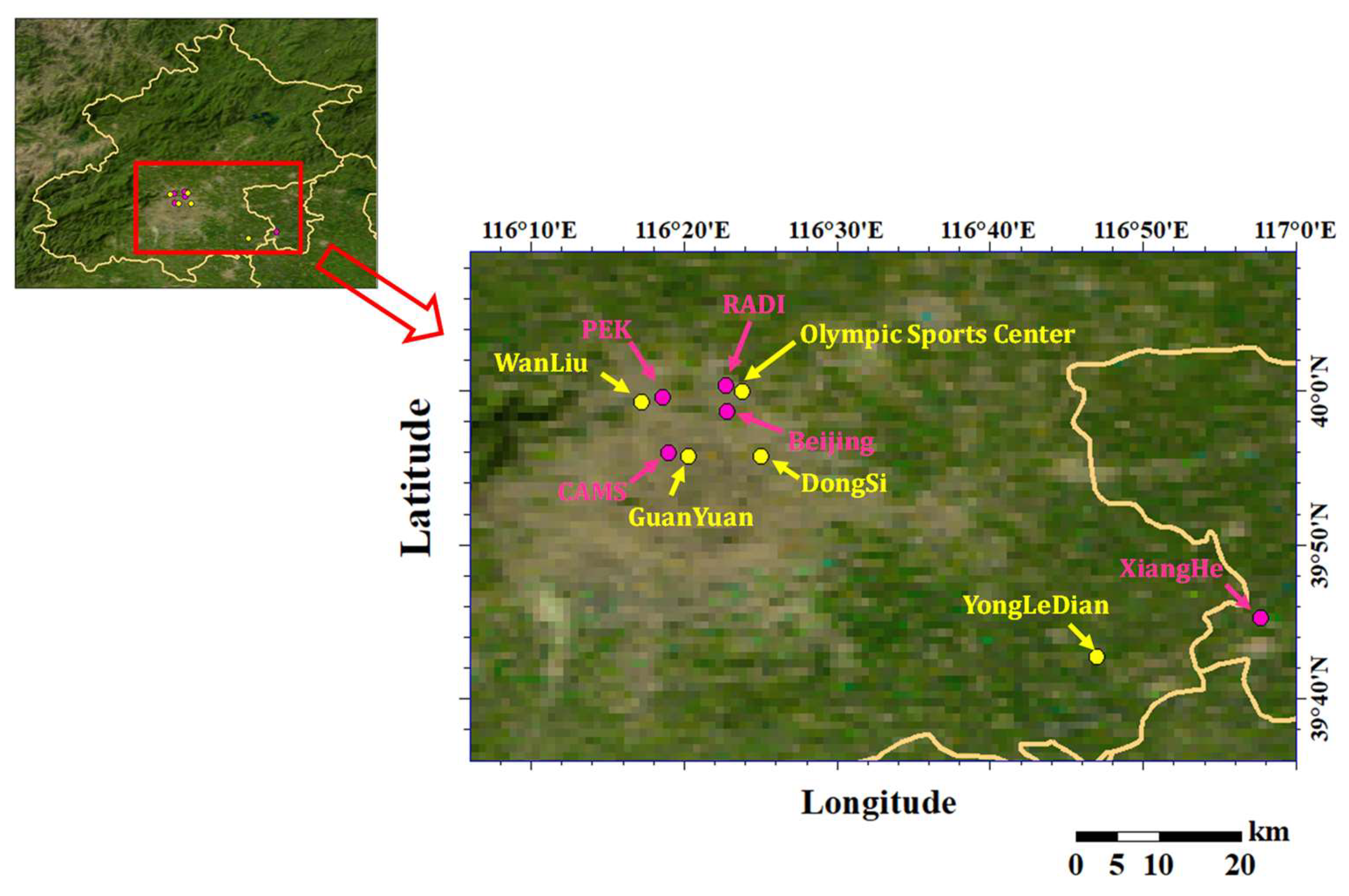
2.5, PBLH and RH reanalyzed by the European Centre for Medium-Range Weather Forecasts (ECMWF), AOD, FMF, particle size distribution, refractive indices from AERONET stations of Beijing area in 2015 were used to establish this model, and datasets of 2016 were used to test the performance of SPSEMCA. The AOD-PM2.5 conversion algorithm based on AERONET data is explained in Section 2. The application results and uncertainty sources of SPSEMCA using AERONET observation data and MODIS monitoring data are shown in Section 3. Section 4 gives the conclusion and possible further improvements to this study.

2. Data and Methods

2.1. Study Area and Data

2.1.1. Ground-Based Stations

Beijing is one of the most important cities in China, with heavy pollution, relatively dense PM monitoring stations and an abundant accessible aerosol observation network data. We selected Beijing as our research area. Five AERONET stations located in the Beijing area, Beijing (116.381°E, 39.977°N), Beijing_CAMS (116.317°E, 39.933°N), PKU_PEK (116.31°E, 39.992°N), Beijing_RADI (116.379°E, 40.005°N), XiangHe (116.962°E, 39.754°N), were selected for this study. Considering the nearest distance and relative location, five PM observation stations were selected from the Beijing Air Quality Monitoring Network (BAQMN), DongSi (116.417°E, 39.929°N), GuanYuan (116.339°E, 39.929°N), WanLiu (116.287°E, 39.987°N), Olympic Sports Center (116.397°E, 39.982°N), YongLeDian (116.783°E, 39.712°N), to pair with the above five AERONET stations, respectively (Figure 1). The distance between the collocated stations is shown in Table 1. The distance of four pairs of matching stations is less than 7 km. The distance between XiangHe and YongLeDian is 16 km. The spatial variation of PM2.5 and the properties of aerosol in the suburbs is less than that of the urban area, so the distance between XiangHe and YongLeDian is acceptable in this study.

2.1.2. Aerosol Properties

The aerosol properties data were collected from two sources; one was AERONET observation, and the other was MODIS (moderate resolution imaging spectroradiometer) products.
We used the newly released Terra and Aqua MODIS collection 6 Multi-Angle Implementation of Atmospheric Correction (MAIAC) 1 km × 1 km 550 nm AOD data with the best quality as input. This product is a MODIS Terra and Aqua combined MAIAC AOD daily Level-2 product (https://lpdaac.usgs.gov/about/news_archive/release_modis_version_6_maiac_data_products) [32]. AOD at 500 nm, the effective radius (EffRad), the particle size distribution, and the Refractive Index at 440 and 675 nm contained in the AERONET Level 1.5 AOD product were also used.
The satellite-based FMF was calculated based on the MODIS LUT-SDA FMF retrieval method [24]. This data was provided by the updated the range of Ångström exponent derivative in the LUT-SDA which is more in line with the seasonal characteristics. The ground-based FMF was extracted from AERONET Level 1.5 SDA (spectral deconvolution algorithm) [33] product.

2.1.3. PM2.5

The hourly ground-level PM2.5 mass concentration was observed by the Beijing Air Quality Monitoring Network and was released by the Beijing Municipal Environmental Monitoring Center (http://www.bjmemc.com.cn/). The ground-level PM2.5 data of Beijing were measured by the tapered element oscillating microbalance method (TEOM); therefore, the PM measured by this method was the dry particle mass concentration.

2.1.4. Meteorological Parameters

Other meteorological parameters, such as the RH and PBLH, were obtained from the ERA-Interim dataset and were reanalyzed by ECMWF, and the resolution was 0.125° × 0.125° (http://apps.ecmwf.int/datasets/data/interim-full-daily/levtype=sfc/). ERA-Interim is a reanalysis of the global atmosphere covering the data-rich period since 1979. This data assimilation system is based on 4-dimensional variational analysis, revised humidity analysis, variational bias correction for satellite data, and other data handling methods [34].

2.1.5. Matching Principle

The ground-based aerosol properties and PM2.5 concentrations were measured at different stations (Figure 1). By assuming that aerosol properties do not vary significantly within 17 km above certain land use types, five couples of AERONET stations and BAQMN stations could be matched (Table 1). Meteorological parameters and satellite aerosol properties were extracted based on locations of BAQMN stations.
To obtain the collocated data, AERONET data were selected between 2:00 and 6:00 (UTC). The averaged PM2.5 and meteorological parameters of 2:00 to 6:00 (UTC) were also used as input data, which corresponds to the transit time of Terra and Aqua at approximately 2:30 and 5:30 (UTC), respectively.
The collocated data from 2015 were used in the model to establish the process, and the data from 2016 were used in PM2.5 retrieval to test the model estimation performance.

2.2. Methodology

Atmospheric particulate matter is an important factor for light extinction. Aerosol optical depth is the column integration of light extinction in the atmosphere. The relationship between AOD and PM2.5 is complex and was affected by the vertical distribution of aerosol, the extinction efficiency, the mass concentration, the microphysical and chemical properties, and the hygroscopicity of aerosol. In this study, we adopted mathematical expressions to fit every conversion process from AOD to PM2.5 and considered multiple parameters.

2.2.1. Particle Correction

PM2.5 refers to the dry mass concentrations of aerosol particles with a diameter of less than 2.5 μm. At the same time, the satellite AOD corresponds to all particle sizes. We used η2.5 (extinction fraction caused by particles with diameter less than 2.5 μm) to make the first step: Particle correction. The total AOD corresponding to all size particles was converted to AOD2.5 (aerosol optical depth related to PM2.5):
AOD 2.5 = AOD × η 2.5 ,
where η2.5 is the extinction fraction corresponding to particles with a diameter less than 2.5 μm, which was obtained by the integration and calculation of the particle size distribution curve and the extinction efficiency curve at 500 nm based on the Mie theory [35], following:
η 2.5 = 0 r 2.5 π Q ext ( r , λ , REF ) r 2 n ( r ) dr 0 π Q ext ( r , λ , REF ) r 2 n ( r ) dr ,
where Qext is extinction efficiency, which is a function of particle radius r, reference wavelength λ = 500 nm, and refractive indices REF; n(r) is the particle numerical size distribution function obtained from AERONET level 1.5 products; r2.5 is the volume equivalent radius corresponding to PM2.5. At the same time, the largest diameter, 2.5 μm for PM2.5, is the aerodynamic diameter, which should be converted into the volume equivalent diameter [21]. Here, we adopt 2.0 μm as the volume equivalent diameter for PM2.5, so r2.5 is equal to 1.0 μm in the above function.

2.2.2. Vertical Correction

AOD2.5 characterizes the extinction of the whole atmosphere, but PM2.5 is measured at the surface level. The PBLH (planetary boundary layer height) was introduced to achieve surface extinction related to less than 2.5 μm diameter particles from AOD2.5. Assuming that aerosols are mainly distributed in PBL, and aerosols in boundary layer are well mixed, the approximation function [28] is as follows:
AOD 0 PBLH σ s dz = σ s PBLH ,
AOD 2.5 0 PBLH σ s , 2.5 dz = σ s , 2.5 PBLH ,
where s means the surface level, z is the height (km), σs and σs,2.5 (km−1) are the surface level extinction coefficient of the total particles and PM2.5, respectively. The vertical correction function AOD2.5/PBLH is used to convert AOD2.5 into the surface extinction coefficient σs,2.5.

2.2.3. Extinction Mass Conversion

PM2.5 is the mass concentration of fine-mode particles. To establish the extinction coefficient and the mass concentration, we introduce the AVEC, the averaged volume extinction coefficient, μm2/μm3, into our model, and then the particle volume per unit volume (V2.5, μm3/μm3) could be achieved as follows:
V 2.5 = σ s , 2.5 / AVEC
AVEC = 0 r 2.5 π Q ext ( r , λ , REF ) r 2 n ( r ) dr 0 r 2.5 4 3 π r 3 n ( r ) dr .

2.2.4. Humidity Correction

V2.5 is the particle volume under ambient conditions, which is the moisture volume of particles and is greatly affected by the ambient relative humidity. In this study, one parameter AMV (the averaged mass volume, cm3/g) is defined to make conversion from V2.5 under moisture conditions to dry particle mass concentrations:
PM 2.5 = V 2.5 / AMV ,
AMV = 0 r 2.5 4 3 π r 3 n ( r ) dr PM 2.5 , m ,
where PM2.5 is the final estimation result of mass concentration corresponding to particle matters with an aerodynamic diameter less than 2.5 μm, and PM2.5, m is the ground level measured particle mass concentration used to establish the retrieval model.

3. Establishing the Model

The methodology described above mainly relies on particle size distribution and refractive indices, which are hard to measure and obtain, and the related dataset is limited. Many other parameters that are easier to access are used to simulate the above parameters, e.g., η2.5, AVEC, and AMV.

3.1. Establishing the PM2.5—AOD Retrieval Model

The conversion from AOD to PM2.5, in this study, goes through several steps: Particle correction, vertical correction, extinction conversion to volume, and humidity correction, and every step includes its fitting process. Finally, when all the fitting steps are synthesized together, the mass concentration of PM2.5 will be obtained. The aerosol property and meteorological data in 2015 were used as the test dataset to establish the retrieval model, and the 2016 data were recognized as the prediction dataset to use for validation.

3.1.1. Particle Correction

Necessity of Particle Correction for the Beijing Area

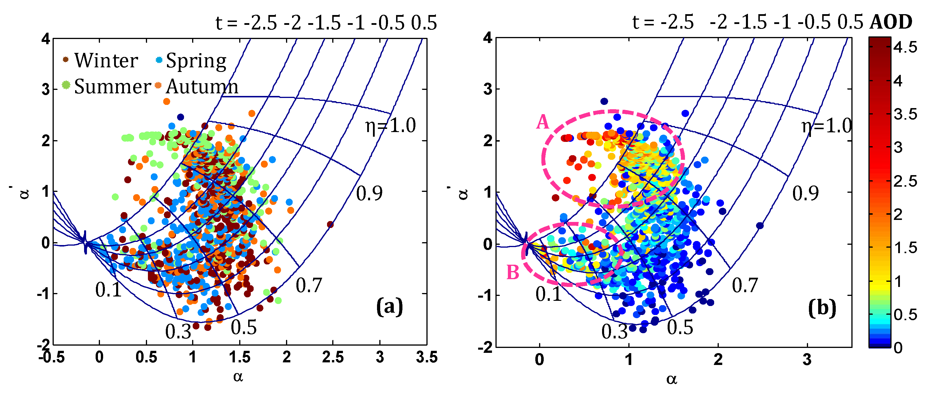
The annual distribution of FMF shows significant seasonal characteristics (Figure 2a). The FMF in spring is obviously lower than that of the other three seasons, while a large majority of samples in summer have high FMF (amasses approximately 0.8). The FMF of samples in autumn and winter was unstable, scattering from 0.1 to 0.95. For a lower FMF, from 0 to 0.5, the AOD decreased with the increase of FMF; then, AOD turned to increase with FMF in a higher range (FMF from 0.5 to 1) (Figure 2b). A large majority of high AOD is contributed to by fine-mode particles, as shown in Figure 2b(A). There also exists the area with lower FMF and higher AOD, as shown in Figure 2b(B), which is mainly caused by dominant coarse-mode particles in aerosol. For instance, a dust storm frequently occurs in spring, which may affect the relationship between AOD and the concentration of fine-mode particles PM2.5. Therefore, using the total AOD to retrieve concentrations of fine-mode particles with a diameter of less than 2.5 μm is somewhat unreasonable.
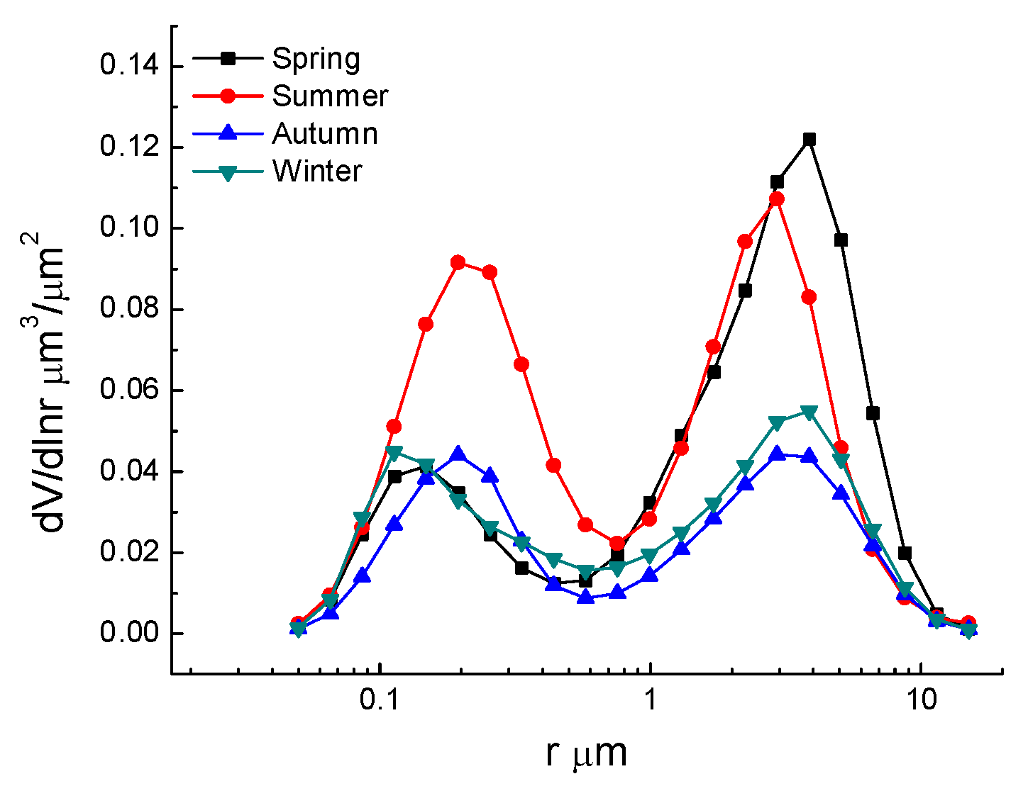
To clarify the stability of FMF, the seasonal particle size distribution of Beijing AERONET station in 2015 is shown in Figure 3. In spring, aerosol is predominated by coarse-mode particles, and the fine-mode fraction is relatively lower, which can also be seen in Figure 2b(B). Summer is a season with high humidity. The moisture in aerosol promotes the secondary transformation of particles, so that the concentration of fine-mode particles is obviously higher than that of other seasons. Meanwhile, with the impact of moisture, aerosol hygroscopic growth accelerates, and the fine-mode median radius of summer aerosol particles is bigger than that of the other seasons. The particle size distribution of winter and autumn is similar.

Method of Particle Correction

As in the above analysis, the concentration and fraction of fine-mode particles is not stable, which shows great differences with the change of season and AOD. AOD is the extinction of all particles, which cannot represent extinction contributed by fine-mode particles. It is a very important process to perform the particle correction and eliminate the impact of coarse-mode particles in the PM2.5-AOD retrieval model. Therefore, we adopted η2.5 to perform particle correction for AOD (Equations (1) and (2)).
However, the calculation of η2.5 relies on refractive indices and the particle size distribution function, which rely on the successful retrieval of the size distribution function based on the size distribution scattering plot. A great amount of computation is required before η2.5 can be obtained, which is time consuming. In this study, we try to use parameters that are contained in ground-based or satellite aerosol products to fit with η2.5, which will bring additional possibilities for the generalization of our retrieval model.
In this paper, we calculated η2.5 based on AERONET particle size distribution and refractive indices data. To avoid introducing large extra uncertainties, the annually averaged refractive indices were used for the input of the Mie calculation for each station. After integration, η2.5 was obtained. It should be noted that the diameter of 2.5 μm refers to the projected area equivalent diameter, which should be converted into the volume equivalent diameter for Mie calculation [35]. Here, η2.5 adopts a specific truncation radius at a volume equivalent to a diameter of approximately 1 μm, which is used as a separation point between fine- and coarse-mode particles. After preliminary experiments, good correlation between the effective radius (EffRad), fine mode fraction (FMF), and η
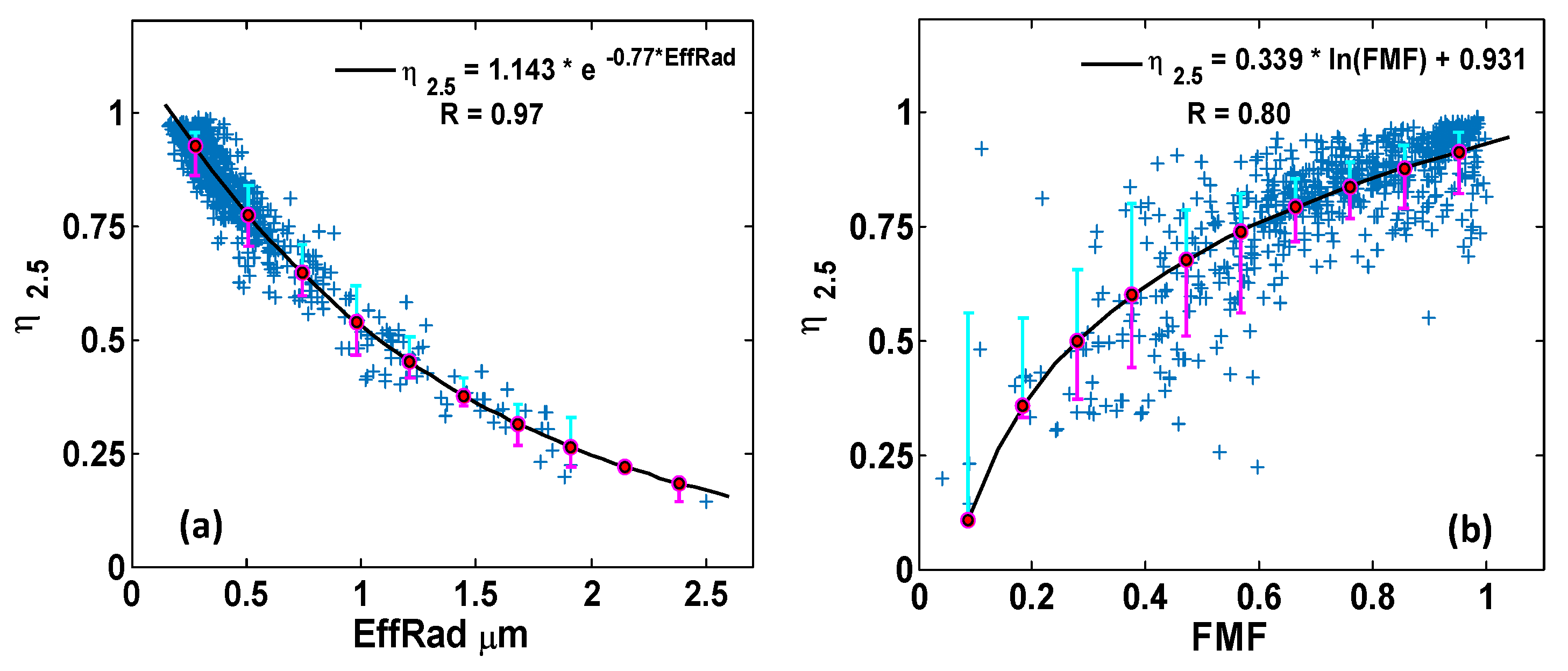
2.5 was found. We use EffRad and SDA FMF to simulate η2.5 based on AERONET data of 2015. As is shown in Figure 4a, η2.5 displays an exponential decline with the increase of EffRad, the fitting line is η2.5 = 1.143 × e(−0.77 × EffRad), and R reaches 0.97. All of the grouped standard deviations are low. The η2.5 increases with FMF (Figure 4b), and the simulation function is η2.5 = 0.339 × ln(FMF) + 0.931, the correlation coefficient is 0.80. The fitting performance for samples with high FMF is good enough. At the same time, the fitting uncertainties are relatively larger for an FMF less than 0.4. Beijing is usually dominated by fine-mode aerosol, and FMF is usually higher than 0.4, so the fitting result is still acceptable. Performing particle correction for ground-based AERONET AOD will adopt an EffRad-η2.5 simulation relationship. Although MODIS does not release EffRad products, we used the FMF-η2.5 fitting line to perform particle correction for the satellite data. Here, AERONET SDA FMF was used to establish the relationship between FMF and η2.5.

3.1.2. Vertical Correction

We used the ECMWF reanalyzed PBLH to perform the vertical correction, converting AOD2.5 to a ground-level extinction coefficient (Equation (4)). We compared the vertical correction performance of ECMWF PBLH with PBLH retrieved based on CALIPSO backscattering data (Figure 5). The extraction of CALIPSO PBLH is based on an algorithm that was proposed by Jordan [36]. This method uses a hybrid standard deviation algorithm, which is more sensitive than the traditional approaches that were used in some cases. In this method, the Haar wavelet and general threshold were employed to approximate the CALIPSO PBLH. As is shown in Figure 5, the CALIPSO PBLH is lower than the ECMWF PBLH as a whole. In winter and spring, they match well, while a significantly higher ECMWF PBLH occurs from May to June. This generally higher ECMWF PBLH will be discussed and adjusted in the following model modification part.
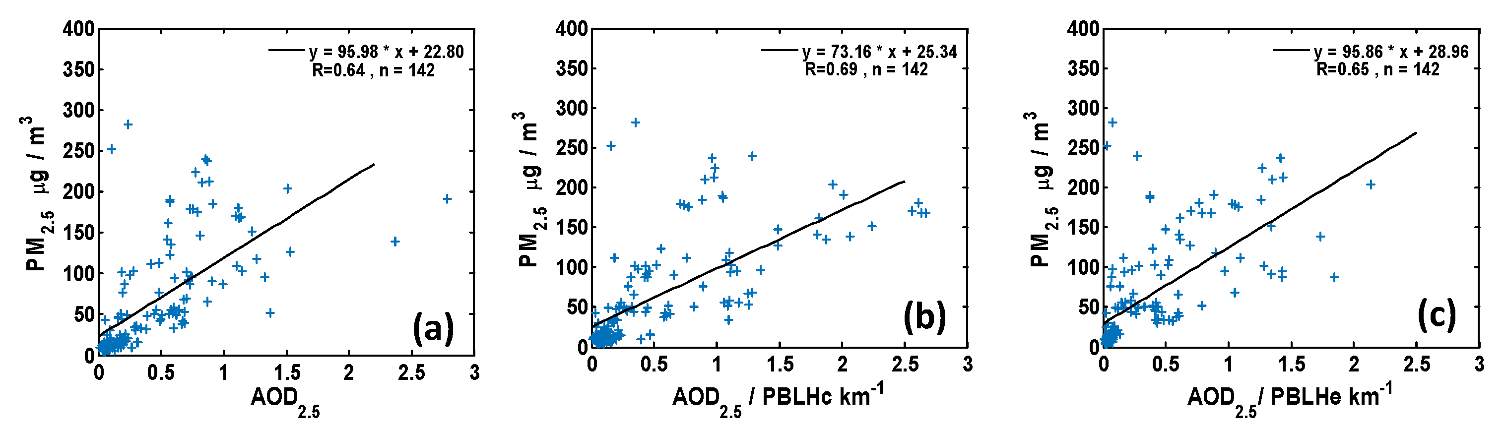
To convert AOD to surface level aerosol extinction, vertical correction is needed. Figure 6 shows the vertical correction results for AOD2.5; both the PBLH from CALIPSO (PBLHc) and from ECMWF (PBLHe) have positive correction effects for the AOD2.5−PM2.5 relationship, and the correlation coefficients are 0.69 and 0.65, corresponding to PBLHc and PBLHe, respectively. As PBLHc is based on CALIPSO actual observation data, the vertical correction performance of PBLHc is better. However, the temporal and spatial coverage of CALIPSO data is limited; therefore, ECMWF reanalyzed PBLH was used to perform the vertical correction, and CALIPSO PBLH was used to perform some adjustment to the model, as is described in the model modification part.

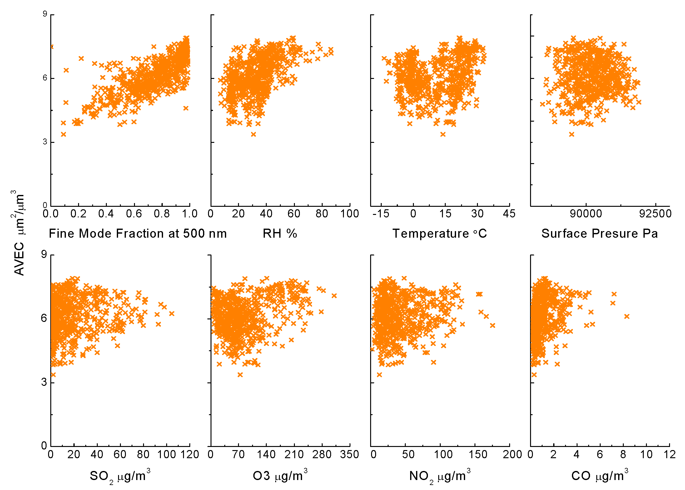
3.1.3. Extinction Conversion to Volume

In this study, we introduce AVEC (averaged volume extinction coefficient, μm2/μm3, Equation (6)), to obtain V2.5 (volume of particle with diameter less than 2.5 μm per unit volume, μm3/μm3, Equation (5)). AVEC is a specific property of aerosol that may be affected by the aerosol composition and surrounding environmental factors. To figure out the influential factors of AVEC, the relationship of AVEC with fine mode fraction at 500 nm, the RH, the temperature, the surface pressure, and the concentration of trace gases (SO2, O3, NO2, CO), are shown in Figure 7. Among the eight parameters, only fine mode fraction at 500 nm and RH has a good liner relationship with AVEC. With the increasing of fine mode fraction at 500 nm and the increasing RH, AVEC presents a linear and logarithm growth trend, respectively. The other six parameters show some relativity with AVEC, but their linear relationship is not very obvious.
Meanwhile, the Pearson correlation test result (Table 2) shows that AVEC is significantly related to fine mode fraction at 500 nm, RH, temperature, SO2, O3, NO2, and CO, at 0.01 level. The correlation coefficient of fine mode fraction at 500 nm, and RH is higher than 0.5.
Considering that the relationships of AVEC with FMF, RH, TM, SO2, O3, NO2, and CO are significant, these seven parameters were used to perform stepwise regression. Using 2015 data to perform this regression, five successful models were obtained (Table 3). Given that the determination coefficient of models 3, 4, and 5 increases little after introducing O3, TM, and CO, we adopt model 2 in Table 3 with predictive variables FMF and RH as the simulation model for AVEC, and the function is AVEC = 3.496 + 2.74 × FMF + 1.9 × (RH/100). To eliminate the impact of the data dimension, we used a standard coefficient to estimate the influence from the predictive variable. The standard coefficients of FMF and RH are 0.629 and 0.29, respectively; in other words, this simulation model is 68% affected by FMF and 32% affected by RH.
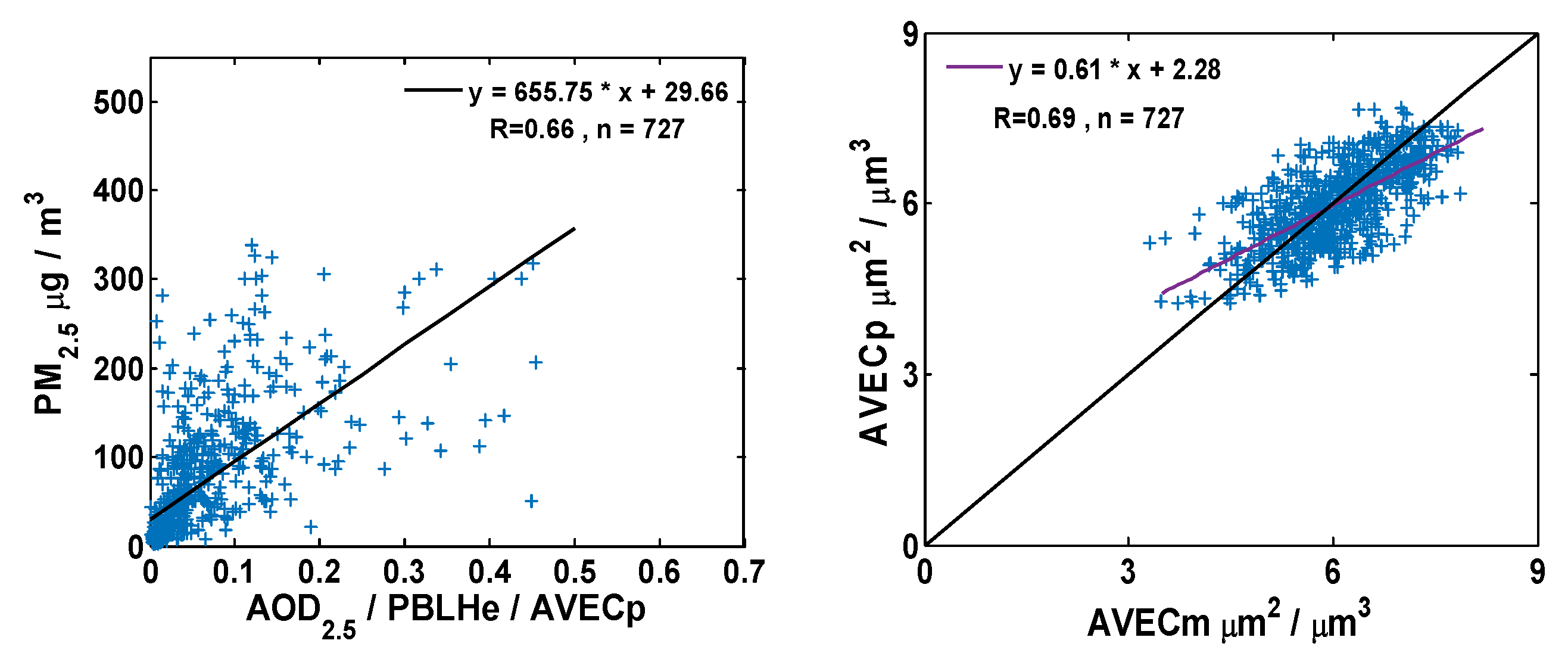
AVEC is simulated in 2016 by introducing FMF and RH. Predicted AVEC fits well with measured AVEC, and the correlation coefficient of the predicted and measured AVEC is 0.69. Then, we used this predicted AVEC to convert the extinction to volume, the relationship of PM2.5 and V2.5 (AOD2.5/PBLHe/AVECp) is distributed as shown in Figure 8, and the correlation coefficient is 0.66.

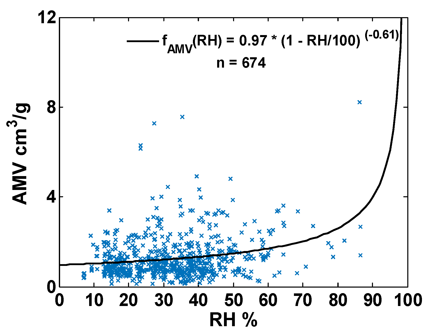
3.1.4. Humidity Correction Using an Empirical Model

In this study, the AMV (averaged mass volume, cm3/g, Equation (8)) is defined to convert V2.5 under moisture conditions into a dry particle mass concentration; in other words, AMV is used to make the humidity correction for V2.5. We adopted the empirical particle hygroscopic growth function [37] as follows:
f AMV ( RH ) = a × ( 1 RH 100 ) b ,
where a and b are parameters of the hygroscopic growth function; here, we used the 2015 data to assimilate these two empirical coefficients.
The simulation results of fAMV(RH) are shown in Figure 9, and have a similar trend as that of the atmospheric particulates hygroscopic growth simulation results of Liu [38] and Wang [31] for the Beijing area. The empirical coefficients a and b are calculated as 0.97 and 0.61, respectively. The large majority of AMV-RH points fit the simulation line, which indicates that the empirical function assimilated for Beijing area is appropriate. AMV increased slowly and near stably when RH was less than 60%, but for high RH situations, the AMV grew exponentially with the increase of RH. Although samples of RH above 60% accounted for a small portion, AMV was varied in a wide range. Appropriate humidity correction is necessary.
Uncertainties of scattered points with AMV > 4 cm3/g and RH < 60% in Figure 9 were analyzed. We found that these points were under a certain boundary layer structure with a high level inversion layer and high surface level wind speed. Surface pollution was lifted upwards and spread with wind. Particle size distribution observed by AERONET could not represent the surface level aerosol properties. This condition is inevitable but rare, which has little influence on the simulation of humidity correction curve. In general, the humidity correction function adopted in this study is efficient.

3.2. Model Modification

Finally, after humidity correction, V2.5 was converted to PM
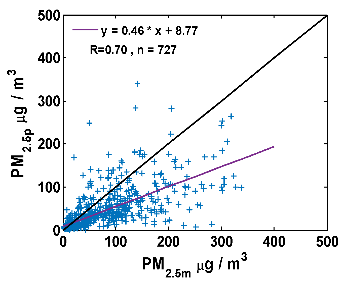
2.5. The distribution of predicted PM2.5 and in situ measured PM2.5 is shown in Figure 10. For all of the 727 matching samples of the Beijing area in 2016, a correlation coefficient of predicted and measured PM2.5 reaches 0.70, which is acceptable. Approximately 79.77% of the 727 matching samples was underestimated, especially for samples with in situ measurement of PM2.5 larger than 200 μg/m3. The slope of the linear regression function is only 0.46.
Particle correction, humidity correction and other conversion are calculated strictly according to AERONET and PM2.5 in situ observation data. Therefore, underestimation may arise during the vertical correction. Furthermore, PBLH obtained from CALIPSO backscattering data and ECMWF reanalysis data did not match very well, as was discussed above. ECMWF re-analyzed PBLH data was used for the PM2.5 prediction, but PBLHe is higher than PBLHc as a whole, which is the main reason for the underestimation of PM2.5.
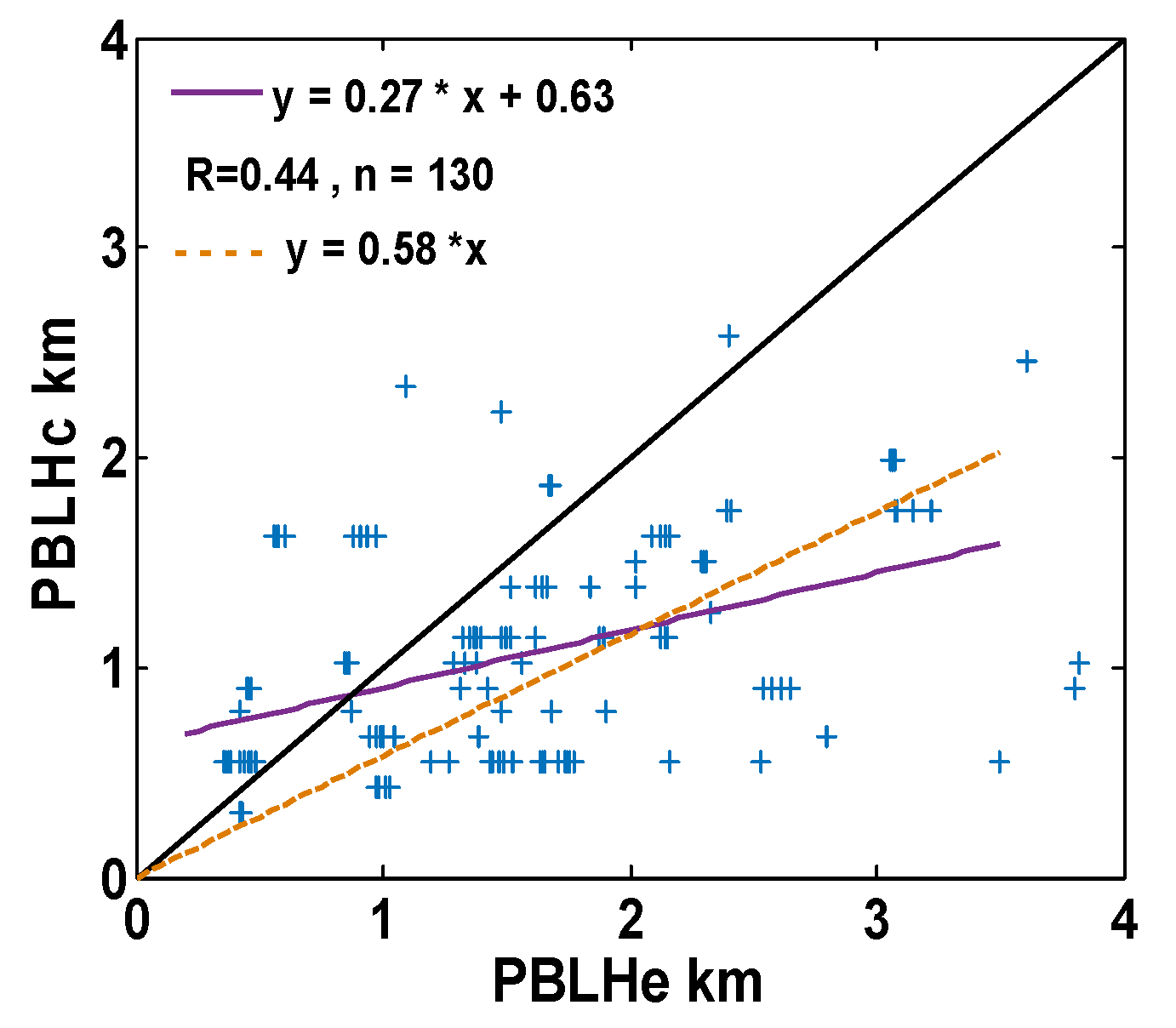
Then, we made an in-depth comparison between PBLHe and PBLHc. The matched PBLHe and PBLHc for the Beijing area in 2015 is distributed in Figure 11. As is shown in the figure, PBLHc ranges from 0 to 2.8 km, while PBLHe ranges from 0 to 4 km. PBLHe is substantially higher than PBLHc, especially for a PBLHe that is larger than 2 km, which is similar to the underestimation trend of PM
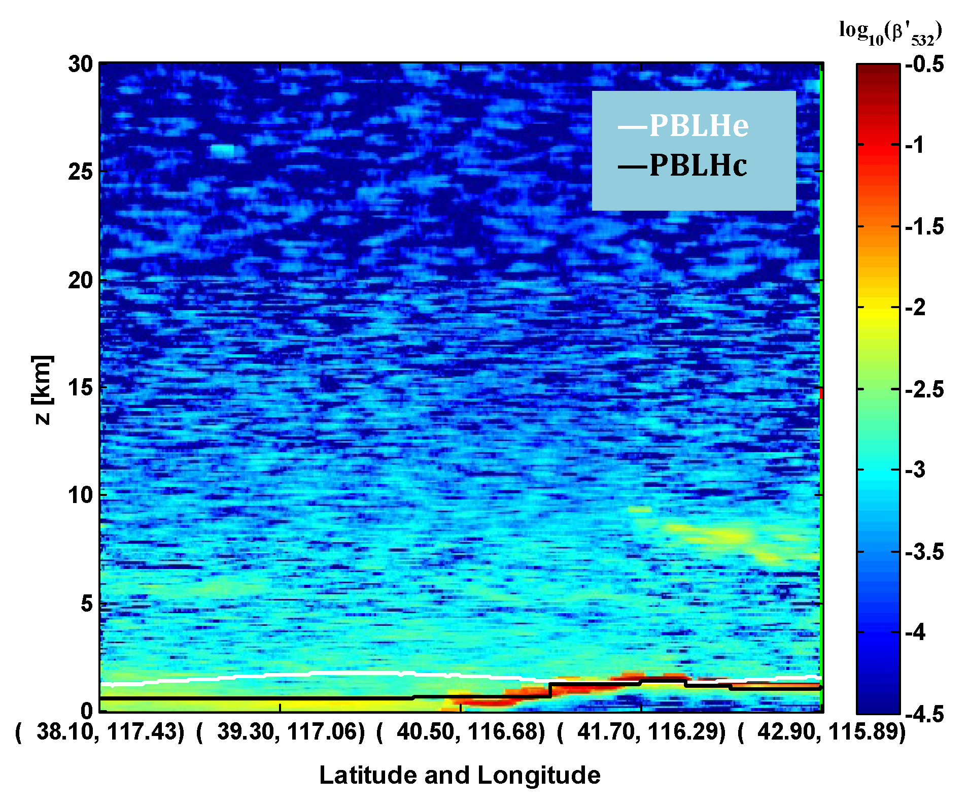
2.5.
Figure 12 shows the CALIPSO backscattering distribution of the Beijing area on February 13, 2015. Aerosol particles mainly spread under 2 km, while particles above 2 km decreased rapidly with the increase of height. Above 4 km, only trace particles could be detected; moreover, its distribution is very smooth. In this figure, the white line indicates PBLH obtained from ECMWF reanalysis datasets, and the black line refers to the PBLH derived from a hybrid standard deviation algorithm using the Haar wavelet and general threshold calculation proposed by Jordan [36]. PBLHc delimits the boundary layer appropriately; under this height, particles are distributed uniformly. However, for south of the CALIPSO transit area, PBLHe is about one times higher than PBLHc, and PBLHe is too high, which should be revised so that it is in line with the actual situation.
We suppose that the interception of the PBLHc-PBLHe regression function is 0; then, the slope of the liner regression function is 0.58. For the sake of uniformity, the magnitude of PBLHe without changing its relative order, PBLHe × 0.58 is used to perform the modification for the above estimation model, and this revised model is the final PM2.5-AOD retrieval method proposed in this study, which is called the specific particle swarm extinction mass conversion algorithm (SPSEMCA).

3.3. Model Error Analysis

The performance of three simulation functions for η2.5, AVEC, and AMV in this paper were tested (Table 4). To obtain a better estimation of the simulation model’s performance and to avoid the influence caused by extreme scattering points, we adopted the median absolute error (AE) and the corresponding relative error (RE) to evaluate the uncertainty of three simulation functions. The median absolute error is approximately 0.030, 0.381 μm3/μm2, 0.465 cm3/g for η2.5, AVEC, and AMV, respectively, based on the modelling dataset of 2015. The averaged relative error of η2.5 and AVEC are lower; both are less than 7%, while uncertainties coming from AMV are relatively high, at approximately 36.6%. Therefore, humidity correction in this study may bring large uncertainties to the final estimation.
According to the error propagation theory, the PM2.5 estimation model suffers from uncertainties of the simulation errors of η2.5, AVEC, and AMV; furthermore, it also comes from the measurement errors of AOD and PBLH, which follow the equation of:
δ PM 2.5 PM 2.5 = ( δ AOD AOD ) 2 + ( δ η 2.5 η 2.5 ) 2 + ( δ PBLH PBLH ) 2 + ( δ AVEC AVEC ) 2 + ( δ f AMV ( RH ) f AMV ( RH ) ) 2 .
The measurement errors coming from observation data δAOD and the reanalysis data δPBLH is difficult to estimate; therefore, we just take η2.5, AVEC, and fAMV(RH) into account. Based on Table 4, η2.5, AVEC, and fAMV(RH) can cause errors at approximately 3.75%, 6.29%, and 36.6%, respectively. According to Equation (10), the total uncertainty caused by parameterization schemes in our specific particle swarm extinction mass conversion algorithm is 37.32%, regardless of the uncertainties caused by the measurement parameters. The uncertainties related to η2.5 and AVEC were approximately 22% as the whole, which indicates that the simulation formulae and relationships found in this study are appropriate and accurate. At the same time, almost all of the other uncertainties were caused by fAMV(RH), which may be affected by the aerosol vertical variation, the measurement error of PM2.5, the reanalysis error of RH, the input uncertainties of V2.5, and the style of the empirical formula that we selected. In the future, the vertical distribution of aerosol will take into consideration, and uniform data sources will be used.

4. Results and Discussion

4.1. PM2.5 Retrieved Results Based on AERONET Data

The final PM2.5 retrieval results for the Beijing area of 2016 based on the AERONET data is shown in Figure 13. Except for some unusual samples, the predicted PM2.5 fits in situ PM2.5 well, the determination coefficient R reaches 0.70 and the RMSE is 58.75 μg/m3, which is acceptable for Beijing, as a heavily polluted area of China. PM2.5 is overestimated for samples with a measured PM2.5 lower than 100 μg/m3. At the same time, PM2.5 is underestimated under heavy PM2.5 loading conditions. The majority of validation samples are under 150 μg/m3. SPSEMCA shows good estimation capability within 150 μg/m3, and the mean RMSE is under 40 μg/m3.
Meanwhile, we analyzed the annually averaged AERONET EffRad, FMF, AOD, and SPSEMCA retrieved PM2.5 of 5 PM2.5 monitoring stations in 2016 (Figure 14). The particle EffRad of 5 stations ranged from 0.41 to 0.57 μm. For the south stations, GuanYuan, DongSi, and YongLeDian, the EffRad are bigger than 0.5 μm. The western and southern stations have higher FMFs, which indicates that the fine-mode particle is the dominant particle in this area. The AOD in western stations, WanLiu and GuanYuan, is higher than that of other stations. The annual mean of the SPSEMCA-retrieved PM2.5 is approximately 60–75 μg/m3. The retrieved PM2.5 of the Olympic Sports Center and YongLeDian is bigger than that of the other three stations. The distribution of PM2.5 is not only affected by AOD but is also related to EffRad and FMF.

4.2. PM2.5 Retrieved Results Based on Satellite Data

Although the ground-based observation of aerosol provides more accurate measurements of AOD and FMF, the spatial coverage is limited. In this study, SPSEMCA is applied to satellite monitoring data. MODIS MAIAC Collection 6 AOD product and MODIS LUT-SDA Fine Mode AOD were used to retrieve satellite-based PM2.5. The validation result of SPSEMCA that was applied to the five BAQMN stations using MODIS data of 2016 is shown in Figure 15. The predicted PM2.5 shows close agreement with the measured value, and the slope of the fitting line is 0.74. Furthermore, the correlation coefficient is 0.75, and the RMSE is 43.38 μg/m3, which is acceptable for Beijing with quite large changes in the PM2.5 all year round. SPSEMCA shows a stable evaluation capacity based on the whole range of measured PM2.5 concentrations. The grouped RMSE for the overestimated samples is lower than that of the underestimated samples.
The MODIS C6 MAIAC AOD, annually averaged MODIS LUT-SDA FM AOD, and SPSEMCA retrieved PM2.5 of the Beijing area are shown in Figure 16. A high AOD is located in the urban area of Beijing and in the north of Tianjin, which is partly different with the high concentration of the PM2.5 area. Fine-mode particles dominated in the south area of Beijing. For the urban area of Beijing, the annual fine mode AOD is above 0.7. The high polluted regions are located in the southeast of Beijing, where the annual average PM2.5 is above 80 μg/m3, which is significantly higher than PM2.5 in the north of Beijing (approximately 40 μg/m3). Compared with other studies, our results show a clear gradient increase trend of PM2.5 from north of Hebei Province to Bohai Bay, which agrees with the study results of Ma et al. [39] based on 2004–2013 (10 years) of mean of estimated PM2.5.
The SPSEMCA PM2.5 retrieval performance based on MAIAC AOD data was tested during a heavily polluted period from October 10 to 14 in the year of 2016 (Figure 17). The measured PM2.5 provided by BAQMN was also shown to validate the performance of SPSEMCA. The heavy pollution was concentrated in southeast Beijing, central Hebei and Tianjin. The spatially distributed trend of the satellite-based PM2.5 fits well with measured PM2.5. The concentration of PM2.5 in southeast Beijing is above 100 μg/m3 and dramatically increased from October 10 to 14, while PM2.5 in the northwest was under 80 μg/m3. This 1 km × 1 km resolution PM2.5 estimation result provides more details about the spatial variation of PM2.5, especially for PM2.5 in rapidly changed areas, as the yellow box shows for October 11. Although PM2.5 increased from 40 to 200 μg/m3 within 20 km in this area, satellite-based PM2.5 retrieval results show the changes clearly, and the estimated value fits well with the measured value of these intensive stations. The result indicates that the algorithm proposed in this paper has practical value for monitoring the area for PM2.5.

4.3. Time Series Analysis of SPSEMCA PM2.5 Retrieved Results for PM2.5 Monitoring Stations

The time-series performances of SPSEMCA based on AERONET and MODIS data for five different PM2.5 monitoring stations are similar. Here, the result for DongSi station is shown (Figure 18). The measured PM2.5 is higher in spring and winter, while it is lower in summer. The predicted PM2.5 based on MODIS and AERONET data fits well with the measured data, apart from several overestimated or underestimated points. The MODIS retrieved PM2.5 performed well during the low PM2.5 loading period, especially under the conditions with a concentration of PM2.5 under 100 μg/m3. PM2.5 estimated by AERONET data is more likely to be overestimated during the high PM2.5 loading period, which may be caused by the uncertainty of AOD and the underestimation of the boundary layer height. We found that the samples with high measured or retrieved AOD (mostly higher than 1) and low RH (mostly lower than 60%) were more likely to be overestimated. The quality of AOD and PM2.5 measurements during the heavy pollution period were an important factor for SPSEMCA. The relationship between AOD, RH, and PM2.5 may need further discussion in heavy pollution cases under dry weather conditions, which is the next step for our future study. Underestimation of PBLH in several cases is another reason for overestimation of PM2.5. In further study, high quality of PBLH datasets assimilated by observation data such as Sounding or Lidar will be tested.

5. Conclusions

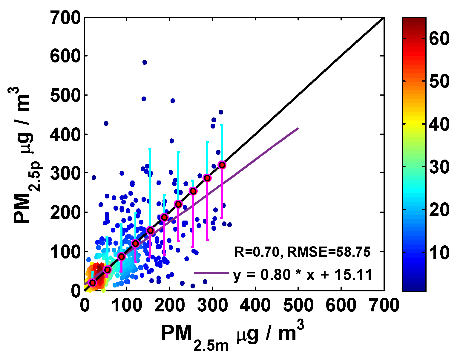
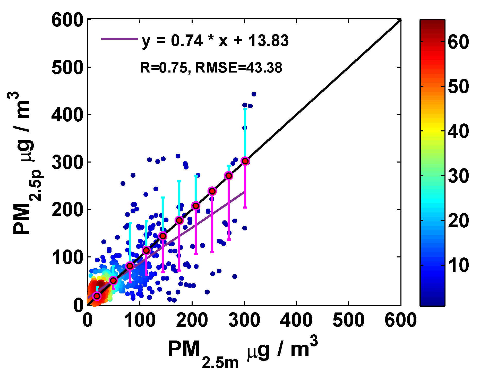
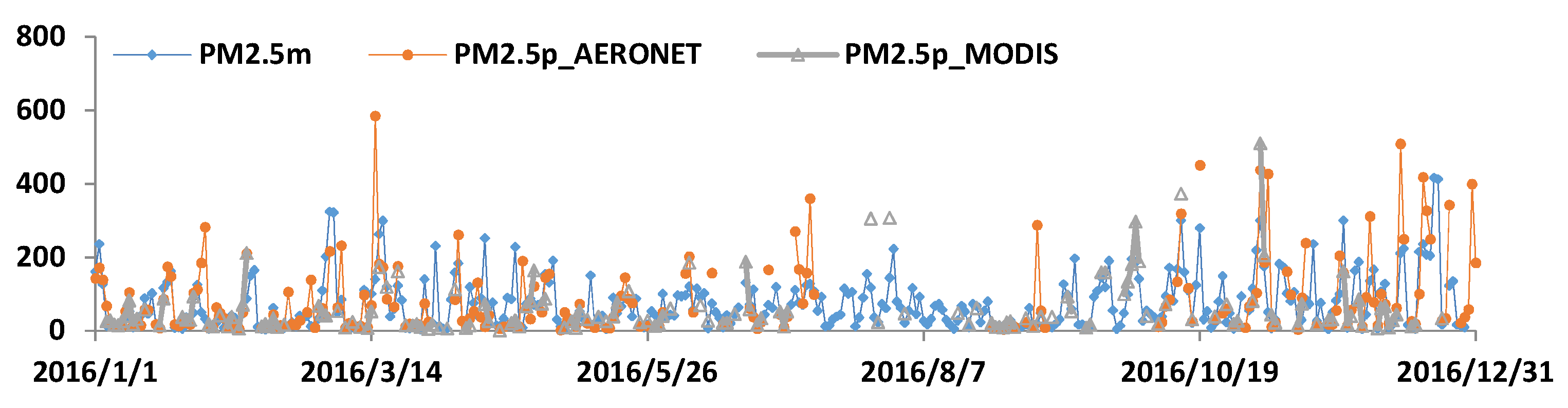
In this paper, a specific particle swarm extinction mass conversion algorithm (SPSEMCA) has been introduced. This method uses particle correction, vertical correction, and humidity correction to successfully convert AOD into PM2.5. Both the applications of SPSEMCA to AERONET observation data and the MODIS monitoring data obtained acceptable results, R = 0.70, RMSE = 58.75 μg/m3 for AERONET data, and R = 0.75, RMSE = 43.38 μg/m3 for MODIS data. These results perform better compared with the results of Zhang [21], R = 0.5, RMSE = 64 μg/m3 based on the MODIS data, with hourly in situ measurements over North China during October–December, 2013. Furthermore, the trend of temporal and spatial distribution of Beijing has been revealed. As for SPSEMCA, there are approximately 37.32% uncertainties that come from the parameterization schemes of η2.5, AVEC, and fAMV(RH). Meanwhile, the satellite application of SPSEMCA suffers large uncertainties from the data quality of FMF, which may lead to the systematic underestimation of PM2.5. Furthermore, the PBLH that was obtained from the ECMWF reanalysis data, which is systematically overestimated compared to the PBLH that was retrieved by CALIPSO backscattering data. A slope modification was made in this paper to rectify this overestimation trend.
This method has five innovation points: (I) We use η2.5 rather than FMF to assimilate AOD2.5, which is contributed to by PM2.5; (II) the assimilation factors of AVEC were selected from eight likely influencing factors and two parameters FMF and RH were finally selected to assimilate AVEC; (III) the performance of PBLH retrieved by satellite Lidar CALIPSO data and a reanalysis by ECMWF were compared in the model establishment process, and CALIPSO PBLH was used to make a systematic correction of the ECMWF PBLH; (IV) we used PM2.5 measured by the ground-based air quality station as the dry mass when calculating the AMV, to avoid the uncertainties derived from the estimation of the particulate matter density ρ; (V) MAIAC AOD with the resolution of 1 km × 1 km AOD was used to retrieve high resolution PM2.5 distribution, and MODIS LUT-SAD FMF was used to avoid the large uncertainties caused by the MODIS FMF product.
In our further study, a consistent source of datasets of PM2.5 and other meteorological parameters should be detected and used. More appropriate linear or nonlinear simulation formulae should be tested to make an accurate humidity correction for PM2.5 retrieving. Vertical correction in SPSEMCA will be improved by detecting more accurate PBLH retrieval methods or high-quality products. Furthermore, an extinction profile monitored by ground-based Lidar is also expected to be used in our future study.

Author Contributions

Y.L. established this AOD-PM2.5 retrieving model, and wrote this paper. Y.X. provided guidance and revised the paper. J.G. provided useful advice for this study. C.F. provided some ideas and technical assistance for this study. S.L. and G.C. provided useful data sources for this paper.

Funding

This work was supported in part by the Ministry of Science and Technology (MOST) of China under grant no. 2016YFC0200500, and the National Natural Science Foundation of China (NSFC) under grant nos. 41471306, 41501385 and 41871260.

Acknowledgments

The LUT-SDA FMF dataset is provided by Dr. Xing Yan. The data for the analysis came from AERONET, MODIS, ECMWF and CALIPSO. We thank the investigators and their staff for establishing and maintaining the important data used in this investigation.

Conflicts of Interest

The authors declare no conflict of interest.

References

  1. U.S. Climate Change Science Program. Atmospheric Aerosol Properties and Climate Impacts; University of North Texas Libraries: Denton, TX, USA, 2009; pp. 2–4. Available online: digital.library.unt.edu/ark:/67531/metadc12022/ (accessed on 12 November 2018).
  2. Jung, J.; Lee, H.; Kim, Y.J.; Liu, X.; Zhang, Y.; Gu, J.; Fan, S. Aerosol chemistry and the effect of aerosol water content on visibility impairment and radiative forcing in Guangzhou during the 2006 Pearl River Delta campaign. J. Environ. Manag. 2009, 90, 3231–3244. [Google Scholar] [CrossRef] [PubMed]
  3. Ding, J.; Zhang, Y.; Han, S.; Xiao, Z.; Wang, J.; Feng, Y. Chemical, optical and radiative characteristics of aerosols during haze episodes of Winter in the North China Plain. Atmos. Environ. 2018, 181, 164–176. [Google Scholar] [CrossRef]
  4. Ramanathan, V.; Crutzen, P.J.; Kiehl, J.T.; Rosenfeld, D. Aerosols, climate, and the hydrological cycle. Science 2001, 294, 2119–2124. [Google Scholar] [CrossRef] [PubMed]
  5. Baker, A.R.; Croot, P.L. Atmospheric and marine controls on aerosol iron solubility in seawater. Mar. Chem. 2010, 120, 4–13. [Google Scholar] [CrossRef] [Green Version]
  6. Chameides, W.L.; Yu, H.; Liu, S.C.; Bergin, M.; Zhou, X.; Mearns, L.; Wang, G.; Kiang, C.S.; Saylor, R.D.; Luo, C.; et al. Case study of the effects of atmospheric aerosols and regional haze on Agriculture: An opportunity to enhance crop yields in China through emission controls? Proc. Natl. Acad. Sci. USA 1999, 96, 13626–13633. [Google Scholar] [CrossRef] [PubMed]
  7. Nazarenko, L.; Rind, D.; Tsigaridis, K.; Del Genio, A.D.; Kelley, M.; Tausnev, N. Interactive nature of climate change and aerosol forcing. J. Geophys. Res. Atmos. 2017, 122, 3457–3480. [Google Scholar] [CrossRef]
  8. Kaufman, Y.J.; Tanré, D.; Boucher, O. A satellite view of aerosols in the climate system. Nature 2002, 419, 215–223. [Google Scholar] [CrossRef] [PubMed]
  9. Krewski, D.; Burnett, R.T.; Goldberg, M.S.; Kristin Hoover, B.; Siemiatycki, J.; Jerrett, M.; Abrahamowicz, M.; White, W. Re-analysis of the harvard six-cities study and the American cancer society study of air pollution and mortality. J. Toxicol. Environ. Health 2003, 66, 1551–1553. [Google Scholar]
  10. Cheng, Z.; Wang, S.; Jiang, J.; Fu, Q.; Chen, C.; Xu, B.; Yu, J.; Fu, X.; Hao, J. Long-term trend of haze pollution and impact of particulate matter in the Yngtze River Delta, China. Environ. Pollut. 2013, 182, 101–110. [Google Scholar] [CrossRef] [PubMed]
  11. Deng, X.; Li, F.; Li, Y.; Li, J.; Huang, H.; Liu, X. Vertical distribution characteristics of PM in the surface layer of Guangzhou. Particuology 2015, 20, 3–9. [Google Scholar] [CrossRef]
  12. Xue, Y.; He, X.; Xu, H.; Guang, J.; Guo, J.; Mei, L. China collection 2.0: The aerosol optical depth dataset from the synergetic retrieval of aerosol properties algorithm. Atmos. Environ. 2014, 95, 45–58. [Google Scholar] [CrossRef]
  13. Kong, L.; Xin, J.; Zhang, W.; Wang, Y. The empirical correlations between PM2.5, PM10 and AOD in the Beijing metropolitan region and the PM2.5, PM10 distributions retrieved by MODIS. Environ. Pollut. 2016, 216, 350–360. [Google Scholar] [CrossRef] [PubMed]
  14. Shao, P.; Xin, J.; An, J.; Kong, L.; Wang, B.; Wang, J.; Wang, Y.; Wu, D. The empirical relationship between PM2.5 and AOD in Nanjing of the Yangtze River Delta. Atmos. Pollut. Res. 2017, 8, 233–243. [Google Scholar] [CrossRef]
  15. Liu, Y.; Wang, Z.; Wang, J.; Ferrare, R.A.; Newsom, R.K.; Welton, E.J. The effect of aerosol vertical profiles on satellite-estimated surface particle sulfate concentrations. Remote Sens. Environ. 2011, 115, 508–513. [Google Scholar] [CrossRef] [Green Version]
  16. Chu, D.A.; Ferrare, R.; Szykman, J.; Lewis, J.; Scarino, A.; Hains, J.; Burton, S.; Chen, G.; Tsai, T.; Hostetler, C.; et al. Regional characteristics of the relationship between columnar AOD and surface PM2.5: Application of lidar aerosol extinction profiles over Baltimore–Washington corridor during DISCOVER-AQ. Atmos. Environ. 2015, 101, 338–349. [Google Scholar] [CrossRef]
  17. Hu, X.; Waller, L.A.; Lyapustin, A.; Wang, Y.; Al-Hamdan, M.Z.; Crosson, W.L.; Estes, M.G.; Estes, S.M.; Quattrochi, D.A.; Puttaswamy, S.J.; et al. Estimating ground-level PM2.5 concentrations in the southeastern united states using MAIAC AOD retrievals and a two-stage model. Remote Sens. Environ. 2014, 140, 220–232. [Google Scholar] [CrossRef]
  18. Lin, C.; Li, Y.; Yuan, Z.; Lau, A.K.; Li, C.; Fung, J.C. Using satellite remote sensing data to estimate the high-resolution distribution of ground-level PM2.5. Remote Sens. Environ. 2015, 156, 117–128. [Google Scholar] [CrossRef]
  19. Chu, D.A.; Kaufman, Y.; Zibordi, G.; Chern, J.; Mao, J.; Li, C.; Holben, B. Global monitoring of air pollution over land from the Earth Observing System-Terra Moderate Resolution Imaging Spectroradiometer (MODIS). J. Geophys. Res. Atmos. 2003, 108, 4661. [Google Scholar] [CrossRef]
  20. Xiao, Q.; Wang, Y.; Chang, H.H.; Meng, X.; Geng, G.; Lyapustin, A.; Liu, Y. Full-coverage high-resolution daily PM2.5 estimation using MAIAC AOD in the Yangtze River Delta of China. Remote Sens. Environ. 2017, 199, 437–446. [Google Scholar] [CrossRef]
  21. Zhang, Y.; Li, Z. Remote sensing of atmospheric fine particulate matter (PM2.5) mass concentration near the ground from satellite observation. Remote Sens. Environ. 2015, 160, 252–262. [Google Scholar] [CrossRef]
  22. Dubovik, O.; Smirnov, A.; Holben, B.N.; King, M.D.; Kaufman, Y.J.; Eck, T.F.; Slutsker, I. Accuracy assessments of aerosol optical properties retrieved from AErosol Robotic NETwork (AERONET) sun and sky radiance measurements. J. Geophys. Res. Atmos. 2000, 105, 9791–9806. [Google Scholar] [CrossRef]
  23. Levy, R.; Remer, L.; Kleidman, R.; Mattoo, S.; Ichoku, C.; Kahn, R.; Eck, T. Global evaluation of the Collection 5 MODIS dark-target aerosol products over land. Atmos. Chem. Phys. 2010, 10, 14815–14873. [Google Scholar] [CrossRef]
  24. Yan, X.; Li, Z.; Shi, W.; Luo, N.; Wu, T.; Zhao, W. An improved algorithm for retrieving the fine-mode fraction of aerosol optical thickness, Part 1: Algorithm development. Remote Sens. Environ. 2017, 192, 87–97. [Google Scholar] [CrossRef]
  25. Yan, X.; Li, Z.; Luo, N.; Shi, W.; Zhao, W.; Yang, X.; Jin, J. A minimum albedo aerosol retrieval method for the new-generation geostationary meteorological satellite Himawari-8. Atmos. Res. 2018, 207, 14–27. [Google Scholar] [CrossRef]
  26. O’Neill, N.T.; Dubovik, O.; Eck, T.F. Modified Angström exponent for the characterization of submicrometer aerosols. Appl. Opt. 2001, 40, 2368–2375. [Google Scholar] [CrossRef] [PubMed]
  27. Yan, X.; Shi, W.; Li, Z.; Li, Z.; Luo, N.; Zhao, W.; Wang, H.; Yu, X. Satellite-based PM2.5 estimation using fine-mode aerosol optical thickness over China. Atmos. Environ. 2017, 170, 290–302. [Google Scholar] [CrossRef]
  28. Koelemeijer, R.B.A.; Homan, C.D.; Matthijsen, J. Comparison of spatial and temporal variations of aerosol optical thickness and particulate matter over Europe. Atmos. Environ. 2006, 40, 5304–5315. [Google Scholar] [CrossRef]
  29. Su, T.; Li, J.; Li, C.; Lau, A.; Yang, D.; Shen, C. An intercomparison of AOD-converted PM2.5 concentrations using different approaches for estimating aerosol vertical distribution. Atmos. Environ. 2017, 166, 531–542. [Google Scholar] [CrossRef]
  30. Cheng, Z.; Ma, X.; He, Y.; Jiang, J.; Wang, X.; Wang, Y.; Sheng, L.; Hu, J.; Yan, N. Mass extinction efficiency and extinction hygroscopicity of ambient PM2.5 in urban China. Environ. Res. 2017, 156, 239–246. [Google Scholar] [CrossRef] [PubMed]
  31. Wang, Z.; Chen, L.; Tao, J.; Liu, Y.; Hu, X.; Tao, M. An empirical method of RH correction for satellite estimation of ground-level PM concentrations. Atmos. Environ. 2014, 95, 71–81. [Google Scholar] [CrossRef]
  32. Lyapustin, A.; Wang, Y. MCD19A2 MODIS/Terra+Aqua Land Aerosol Optical Depth Daily L2G Global 1km SIN Grid V006 [Data Set]; NASA EOSDIS Land Processes DAAC: Boulder, CO, USA, 2018. [Google Scholar]
  33. O’Neill, N.; Eck, T.; Smirnov, A.; Holben, B.; Thulasiraman, S. Spectral discrimination of coarse and fine mode optical depth. J. Geophys. Res. Atmos. 2003, 108, 4559–4562. [Google Scholar] [CrossRef]
  34. Berrisford, P.; Dee, D.P.; Poli, P.; Brugge, R.; Mark, F.; Manuel, F.; Kållberg, P.W.; Kobayashi, S.; Uppala, S.; Adrian, S. The ERA-Interim Archive Version 2.0; ECMWF: Reading, UK, 2011; pp. 3–10. [Google Scholar]
  35. Hand, J.L.; Kreidenweis, S.M. A new method for retrieving particle refractive index and effective density from aerosol size distribution data. Aerosol Sci. Technol. 2002, 36, 1012–1026. [Google Scholar] [CrossRef]
  36. Jordan, N.S. Validation of the Version 5 Goddard Earth Observing System (GEOS-5) Using Cloud-Aerosol Lidar and Infrared Pathfinder Satellite Observations (CALIPSO); University of Maryland: Baltimore County, MD, USA, 2009. [Google Scholar]
  37. Kotchenruther, R.A.; Hobbs, P.V.; Hegg, D.A. Humidification factors for atmospheric aerosols off the mid-Atlantic coast of the United States. J. Geophys. Res. Atmos. 1999, 104, 2239–2251. [Google Scholar] [CrossRef] [Green Version]
  38. Liu, X. Observation and Modeling Study of Atmospheric Aerosol Hygroscopic Properties—Taking Beijing and Zhujiang Delta as an Example. Ph.D. Thesis, Peking University, Beijing, China, 2008. [Google Scholar]
  39. Ma, Z.; Hu, X.; Sayer, A.M.; Levy, R.; Zhang, Q.; Xue, Y.; Tong, S.; Bi, J.; Huang, L.; Liu, Y. Satellite-based spatiotemporal trends in PM2.5 concentrations: China, 2004–2013. Environ. Health Perspect. 2016, 124, 184–192. [Google Scholar] [CrossRef] [PubMed]
Figure 1. Locations of AErosol Robotic NETwork (AERONET) stations and air quality monitoring stations in the Beijing area.
Remotesensing 10 01906 g001
Figure 2. Aerosol properties distribution for different seasons and aerosol optical depth (AOD) levels (reference wavelength of λ = 500 nm) of five AERONET stations in the year 2015 (n = 975). Different colors in (a) refer to different seasons; and in Figure 2b refer to different AOD levels. The circle A and B in (b) refer to different type of samples. α, α′, η, refers to the Angstrom coefficient, the instantaneous slope of α versus lnλ, fine mode fraction, t is an intermediate variable in η retrieving based on the spectral deconvolution algorithm (SDA) [33].
Remotesensing 10 01906 g002
Figure 3. Particle size distribution for different seasons of Beijing station in 2015.
Remotesensing 10 01906 g003
Figure 4. Simulation of η2.5 (extinction fraction caused by particles with a diameter less than 2.5 μm) by introducing the effective radius or fine-mode fraction (FMF). The subfigure (a) refers to η2.5 simulation result for PM2.5 retrieval based on AERONET data; subfigure (b) refers to η2.5 simulation result for PM2.5 retrieval based on MODIS data. The blue-green error bars represent the mean standard deviation for samples above the fitting line; the magenta error bars represent the mean standard deviation for samples under the fitting line; the magenta points on the fitting line represent group centers.
Remotesensing 10 01906 g004
Figure 5. CALIPSO planetary boundary layer height (PBLH) and the European Centre for Medium-Range Weather Forecasts (ECMWF) PBLH of Beijing station in 2016.
Remotesensing 10 01906 g005
Figure 6. Vertical correction performance with PBLH from CALIPSO (PBLHc) and ECMWF (PBLHe).
Remotesensing 10 01906 g006
Figure 7. Relationship of averaged volume extinction coefficient (AVEC) with eight likely influence factors (year = 2015, n = 637).
Remotesensing 10 01906 g007
Figure 8. AVEC simulation results and particulate matter (PM)2.5-V2.5 relationship (year = 2016, n = 727).
Remotesensing 10 01906 g008
Figure 9. Simulation results of fAMV(RH) for the Beijing area.
Remotesensing 10 01906 g009
Figure 10. Validation results of predicted PM2.5 and in situ measured PM2.5.
Remotesensing 10 01906 g010
Figure 11. Comparison of PBLHe and PBLHc for the Beijing area in 2015.
Remotesensing 10 01906 g011
Figure 12. CALIPSO backscattering distribution and PBLH of the Beijing area on 13 February 2015.
Remotesensing 10 01906 g012
Figure 13. Validation result of the specific particle swarm extinction mass conversion algorithm (SPSEMCA) for Beijing area in 2016. The color bar from 0 to 60 represents the sample density. The blue-green error bars represent mean root mean square error (RMSE) for samples with estimated PM2.5 larger than the measured value (samples above the 1:1 line); the magenta error bars represent the mean RMSE for samples with estimated PM2.5 lower than the measured value (samples under the 1:1 line); the magenta points on the 1:1 line represent group centers.
Remotesensing 10 01906 g013
Figure 14. The annually averaged AERONET EffRad, FMF, AOD, and SPSEMCA retrieved PM2.5 of five PM2.5 monitoring stations in 2016.
Remotesensing 10 01906 g014
Figure 15. Validation result of satellite application with SPSEMCA of the Beijing area in 2016. The color bar from 0 to 60 represents the sample density. The blue-green error bars represent the mean RMSE for samples with estimated PM2.5 that are larger than the measured value (samples above the 1:1 line); the magenta error bars represent the mean RMSE for samples with estimated PM2.5 lower than the measured value (samples under the 1:1 line); the magenta points on the 1:1 line represent group centers.
Remotesensing 10 01906 g015
Figure 16. The annually averaged MODIS Multi-Angle Implementation of Atmospheric Correction MAIAC AOD, MODIS fine mode (FM) AOD, and SPSEMCA retrieved PM2.5, of the Beijing area in 2016.
Remotesensing 10 01906 g016
Figure 17. Performance of SPSEMCA during a heavily polluted period in the Beijing area, 2016. Points refer to the ground-based PM2.5 measurement stations from BAQMN; the color and size of the points refer to the concentration of PM2.5.
Remotesensing 10 01906 g017
Figure 18. Time series distribution of SPSEMCA PM2.5 retrieved result for DongSi PM2.5 monitoring station based on AERONET and MODIS data, PM2.5m means PM2.5 measured by the Beijing Air Quality Monitoring Network; PM2.5p_AERONET means the SPSEMCA predicted PM2.5 based on the AERONET dataset; PM2.5p_MODIS means the SPSEMCA predicted PM2.5 based on MODIS dataset.
Remotesensing 10 01906 g018
Table 1. The distance between paired stations.
AERONET StationBAQMN StationDistance
BeijingDongSi6.16 km
Beijing_CAMSGuanYuan1.93 km
PKU_PEKWanLiu2.04 km
Beijing_RADIOlympic Sport Center2.98 km
XiangHeYongLeDian16.00 km
Table 2. Pearson correlation coefficient of AVEC with eight likely influence factors.
ParametersFMFRHSPTMSO2O3NO2CO
AVEC0.736 **0.522 **−0.0190.233 **0.135 **0.310 **0.006 **0.255 **
** indicate the significance level of 0.01.
Table 3. Stepwise regression results with seven likely influence factors.
ModelR2RMSE
1. FMF0.540.594
2. FMF, RH0.620.545
3. FMF, RH, O30.640.526
4. FMF, RH, O3, TM0.650.519
5. FMF, RH, O3, TM, CO0.650.515
Table 4. Median absolute error (AE) and the corresponding relative error (RE) of three estimation functions.
ParametersAERE%
η2.50.0303.75
AVEC μm3/μm20.3816.29
AMV cm3/g0.46536.6

