Ocean Wind Retrieval Models for RADARSAT Constellation Mission Compact Polarimetry SAR

Abstract

We propose two new ocean wind retrieval models for right circular-vertical (RV) and right circular-horizontal (RH) polarizations respectively from the compact-polarimetry (CP) mode of the RADARSAT Constellation Mission (RCM), which is scheduled to be launched in 2019. For compact RV-polarization (right circular transmit and vertical receive), we build the wind retrieval model (denoted CoVe-Pol model) by employing the geophysical model function (GMF) framework and a sensitivity analysis. For compact RH polarization (right circular transmit and horizontal receive), we build the wind retrieval model (denoted the CoHo-Pol model) by using a quadratic function to describe the relationship between wind speed and RH-polarized normalized radar cross-sections (NRCSs) along with radar incidence angles. The parameters of the two retrieval models are derived from a database including wind vectors measured by in situ National Data Buoy Center (NDBC) buoys and simulated RV- and RH-polarized NRCSs and incidence angles. The RV- and RH-polarized NRCSs are generated by a RCM simulator using C-band RADARSAT-2 quad-polarized synthetic aperture radar (SAR) images. Our results show that the two new RCM CP models, CoVe-Pol and CoHo-POL, can provide efficient methodologies for wind retrieval.

1. Introduction

The Canadian RADARSAT Constellation Mission (RCM) is scheduled for launch in early 2019 and will provide Compact-Polarimetry (CP) synthetic aperture radar (SAR) data. RCM is the evolution of the RADARSAT Program and the successor of RADARSAT-2, which is a satellite constellation carrying three identical C-band SAR satellites. The RCM CP mode consists of a right hand circular transmit and linear/circular receive radar signal, namely right circular-vertical (RV) polarization, right circular-horizontal (RH) polarization, right circular-right circular (RR) polarization and right circular-left circular (RL) polarization. The CP configuration is designed for Earth observation; compared with conventional linear dual-polarization SAR, compact polarimetry SAR can obtain abundant high-resolution information with wider swath [1].

Researchers have shown that CP SAR is an efficient imaging mode for ocean surface observation and, therefore, elucidation of algorithms and models for retrieval of ocean surface features and marine variables like wind is critically important [2]. Compact polarization SAR is a dual-polarization radar system which transmits circular (or 45°) components and receives two orthogonal polarization components (V or H) with relative phase [3,4]. Accurate information of ocean surface can be obtained from C-band radar data. The main process of physical mechanism is the interactions between the microwaves and related surface water waves. The major interaction is denoted as Bragg scattering when the wavelengths of ocean surface waves are of the same order of radar wavelength. For practical application, wind retrievals from SAR images can be accomplished by C-band geophysical model functions (GMFs), because radar measurements are sensitive to the ocean-surface roughness which is determined by the surface wind field [5]. The GMF is a set of functions between wind vectors and radar backscatter signals denoted as the normalized radar cross section (NRCSs) including dependence on the radar incidence angles.

The C-band GMF model series (CMOD4, CMOD5 and CMOD5.N [5,6]) are used for vertical-vertical (VV) polarization data. For horizontal-horizontal (HH) polarization, there are generally two ways to achieve ocean wind retrieval: (1) conversion of the HH backscatter to VV by a polarization ratio (PR) which is a ratio of VV-polarized NRCS to HH-polarized NRCS [7], or (2) construction of a new relationship between wind vectors and radar backscatters [8]. In terms of C-band linear cross-polarization (VH and HV) ocean backscatter data, C-2PO and C-3PO models are available for wind retrieval [9,10]. For wind retrieval from CP SAR mode, recent studies have attempted to retrieve wind speed by converting right circular-vertical (RV) polarization data into linear dual-polarization data, taking advantage of CMOD5 and CMOD5.N models [11,12]. However, the configurations for RV and VV polarizations are different and the CMOD model series were originally developed for C-Band VV-polarized scatterometers rather than SARs. In view of this situation, we propose two new models in this paper to retrieve wind from C-band RV-pol and RH-pol measurements.

CMOD is a well-behaved parameterization to retrieve wind speed, allowing the NRCS to be dependent on the principal parameters, such as radar incidence angle, relative wind direction and wind speed [5]. However, as there are 28 CMOD coefficients, the process of optimizing the CMOD model to CP data sets to generate a new GMF (for CP SAR) is not feasible using normal computing clusters, because of the requirement to adjust such large number of CMOD coefficients to represent the CP parameters. In order to avoid excessive computation, a sensitivity analysis of the coefficients can play a significant role in optimizing the generation of a new GMF for RV-polarization. The sensitivity analysis is a method to adjust the models by changing the coefficients within a specific range of variations in order to optimize the parameterization and simplify the computation [13,14]. Moreover, another common method to generate a practical empirical algorithm is to fit a function relating the CP variables and the wind parameters. In this study, we utilize these two methods to construct the wind speed retrieval models for RV- and RH-polarization data.

RADARSAT-2 is beyond its 7-year design life, as it was launched in 2007. Thus the launch of RCM is necessary, and application of CP SAR is a new application offering the advantages of full polarimetry SAR mode, with the possibility of better wide-swath coverage. Based on the simulated CP parameters, this study is a preparation for possible ocean wind retrievals from RCM which will be available in the next year. The remainder of this paper is organized as follows: Section 2 describes the database consisting of CP SAR NRCSs simulated by the RCM simulator using quad-polarized RADARSAT-2 SAR images, and collocated wind vectors observed by NCBC buoys. A new CMOD function for RV-polarization data is proposed based on a sensitivity analysis [13], followed by a performance evaluation, and we present a new model for RH polarization wind speed retrieval. Results and the validations of the two new models are shown in Section 3. Discussion and conclusions are given in Section 4 and Section 5, respectively.

2. Materials and Methods

In this section, two wind retrieval models are developed based on the collocated data sets. For the compact RV polarization, we employ the CMOD framework to derive a new GMF by optimizing each coefficient. The resultant formulation is denoted the CoVe-Pol model. In this derivation, sensitivity analysis is used to avoid unnecessarily huge calculations [13]. Through the sensitivity analysis, the computation efficiency of the process to generate the new GMF generation is increased by more the 10²⁰ times and the accuracy of computed NRCS reaches 10⁻². For the compact RH polarization, we propose the CoHo-Pol wind retrieval model which we derive by using a quadratic regression function.

2.1. Datasets

The CP parameters were simulated from RADARSAT-2 quad-polarized data using the RCM simulator, which is provided by the Canadian Space Agency [12]. To develop two new wind retrieval models for RV- and RH-polarization data, we build a database consisting of simulated RV- and RH-polarized NRCSs from RADARSAT-2 fine quad-pol SAR images and collocated wind vectors measured by in situ buoys. The RADARSAT-2 quad-pol SAR images over the selected buoys are acquired. Then, these RADARSAT-2 images are converted to RCM CP mode SAR images by using the CP simulator. Finally, wind speed measured by buoy and the collocated simulated NRCS are paired. The distributions of NRCSs and wind speeds are shown in Figure 1.

In this database, we have 267 RADARSAT-2 fine quad-pol SAR images, which are processed by a RCM CP simulator to re-construct CP mode images [1]. The results of simulated CP configurations are used as “ground truth” in this study. The RADARSAT Constellation Mission has several polarization configurations: linear mono-polarized, dual linear-polarized (HH/HV, VV/VH, or VV/HH); dual circular transmit-linear receive; and fully polarimetric [12]. The compact polarimetry SAR mode provides four polarimetric datasets, which are RV, RH, right circular transmit and right circular receive (RR) and right circular transmit and left circular receive (RL). In the medium resolution mode, the pixel spacings in azimuth and range directions are about 100 m and the associated noise floor is about −25 dB [15]. Data from eight National Data Buoy Center (NDBC) buoys collocated with the SAR data are collected, at locations off the east and west coasts of Canada [16]. The buoy locations are shown in Figure 2. At each buoy, the mean wind speed (at 10 m reference height, hereafter U₁₀) and direction are measured by two sensors, averaged over 8-min periods and reported hourly. The wind speeds observed by the buoys are converted to winds at 10 m reference height above the ocean surface using the Tropical Ocean and Global Atmosphere Coupled Ocean-Atmosphere Response Experiment (TOGA COARE) bulk flux algorithm [17], and the winds can be considered as neutral winds [6,18]. The temporal separation between the SAR data and the buoy data is restricted to less than 30 min [11]. The distribution of months is shown in Figure 3. As the SAR is active microwave, the effects of weather and seasons are both almost negligible.

We divide the collected data randomly into two data groups (2/3 and 1/3 of the total number). One contains 178 data which are used to generate the new models, and the other contains 89 data, reserved for model testing.

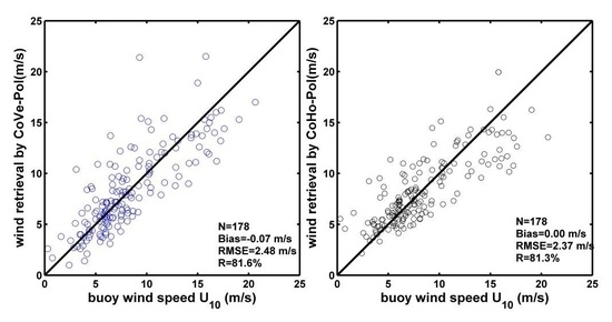
2.2. CoVe-Pol Model for Right Circular-Vertical (RV) Polarization

Figure 4 shows the flowchart for the derivation process for the CoVe-Pol model for RV polarization data. As with all GMF functions, an empirical functional relation is used to establish the dependency of the normalized backscatter on wind speed, wind direction, and the incidence angle [5]. The general form of the CMOD function is summarized as:

$$\begin{array}{l}{\sigma }^0(\theta ,U_{10},\phi )=\\ B0(c_0,U_{10},\theta ){[1+B1(c_1,U_{10},\theta )\cos (\phi )+B2(c_2,U_{10},\theta )\cos (2\phi )]}^{1.6}\end{array}$$

(1)

where σ⁰ is the NRCS in linear units, φ is the relative wind direction, which is the angle between local wind direction and radar look direction (both relative to north), U₁₀ is the statistically neutral wind referenced to 10 m height, θ is the incidence angle and B0, B1, B2 are coefficients depending on U₁₀, θ, the radar frequency and polarization. The dominant term, B0, sets the speed scale for a given measurement. The upwind–crosswind asymmetry term B2 allows for a determination of the wind direction, and B1 is used to resolve the remaining 180° ambiguity in the wind direction. Coefficients c_i complete the definition of the terms B0, B1, B2. Detailed expressions are shown in Appendix A.

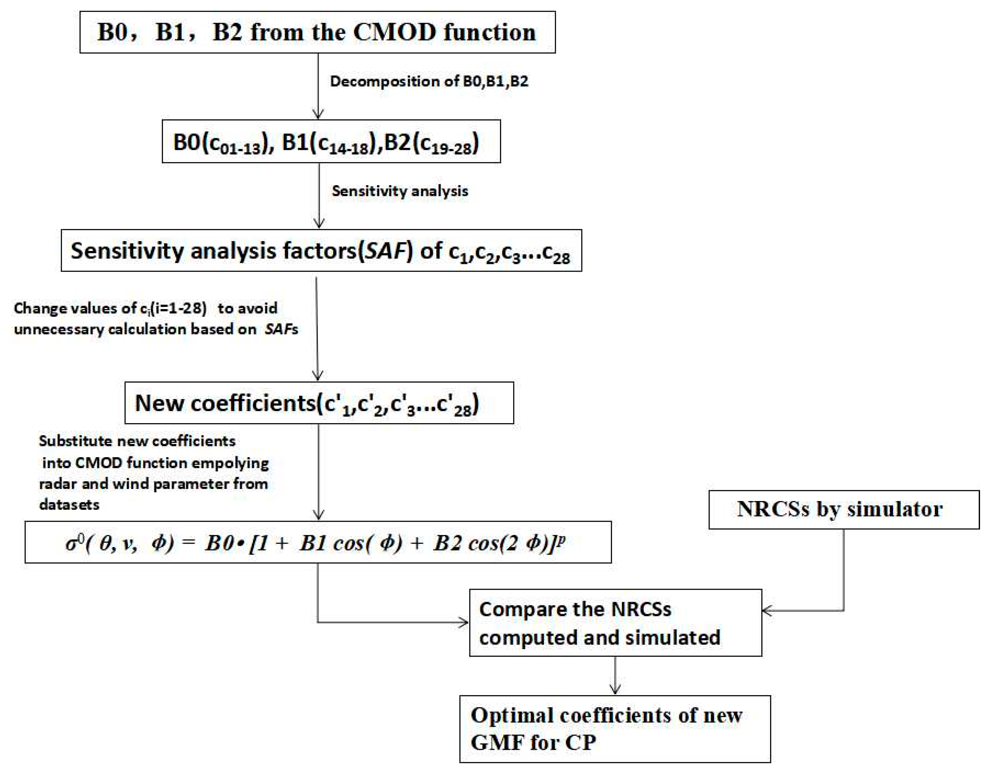
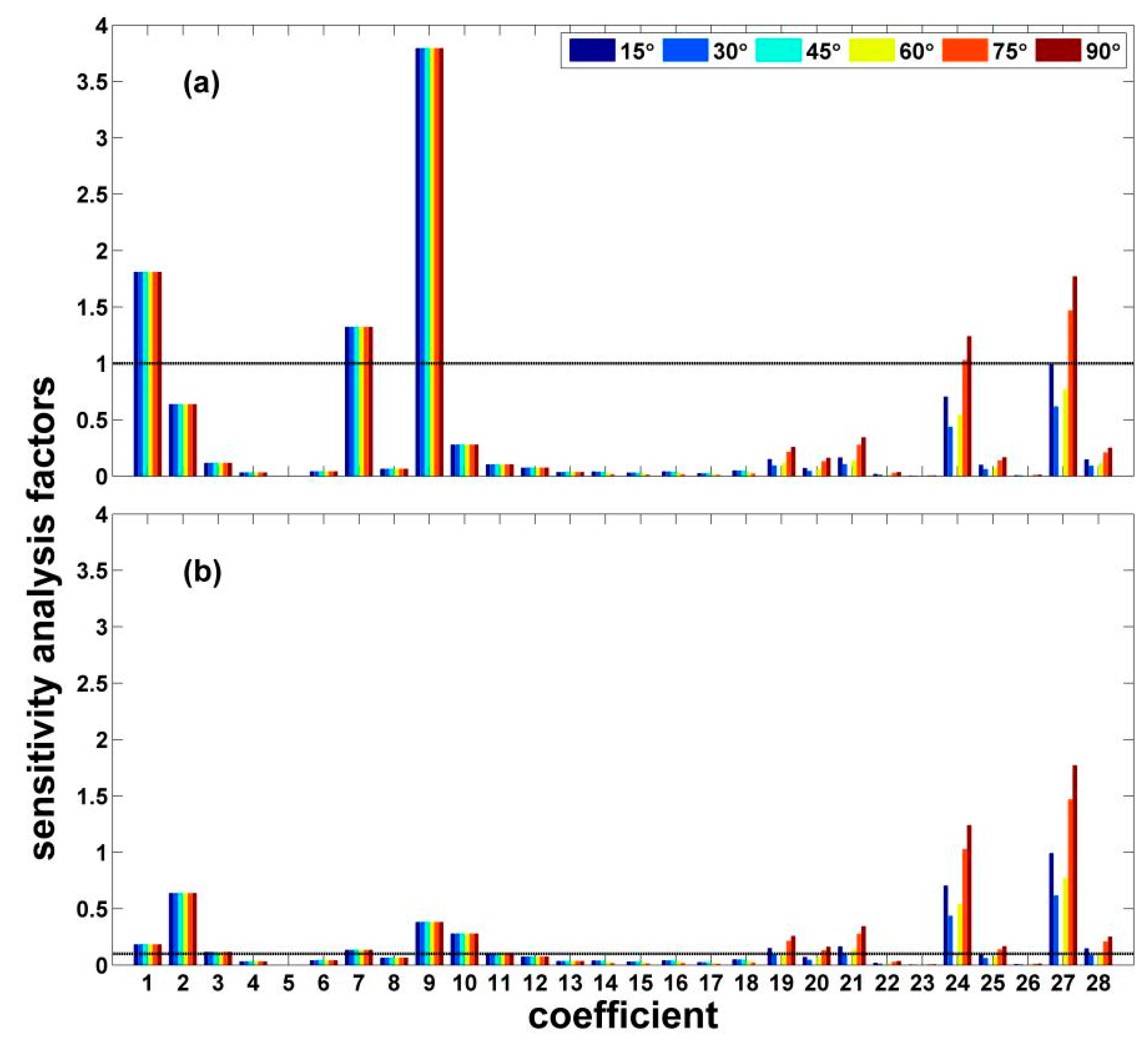
2.2.1. Sensitivity Analysis

As there are 28 CMOD coefficients (c₁~c₂₈) in the empirical model formulation, the sensitivity analysis is used to reduce the computations and to allow a determination of the coefficients. We define the sensitivity analysis factor (SAF) of the CMOD coefficients to make the adjustment process more efficient:

$$SAF=\left|(\delta {\sigma }^0/{\sigma }^0)/(\delta c_i/c_i)\right|$$

(2)

where σ⁰ represents the RV-polarized backscatter value (NRCS), the independent variable, and the c_i coefficients (c₁~c₂₈) are dependent variables. In this approach, SAFs indicate the degree of influence of each coefficient on the CMOD parameterization. From equation (2), we know that for any particular coefficient c_i, the corresponding NRCS (σ⁰) can have multiple values, and in each case the ratio is indicative of the degree of influence, SAF. If SAF cannot provide the required computational accuracy, the corresponding coefficients c_i can be ignored. For any particular coefficient, the basis for this decision is the magnitude of the degree of influence, SAF.

Average values of the SAFs under various wind speeds range from 1 m/s to 25 m/s as shown in Figure 5, assuming typical conditions for radar incidence angles and wind directions. Thus, it is shown that SAF values range widely from 0 to 10¹, which means the influence of different coefficients, c_i, vary greatly. As shown in Figure 5, very close to 0, most SAF values are less than 1 and only a few have values exceeding 1, for three typical radar incidence angles (25°, 35° and 45°). Thus, we only focus on coefficients c_i, where SAF values indicate greater influence (>0.1) so that the parameterization is simplified and a huge calculation can be avoided.

In this study, we can classify the coefficients by the orders of magnitude of the corresponding SAFs, namely 10⁰, 10⁻¹ and less than 10⁻¹. Thus, when we attempt to get the accuracy of computed NRCS values to 10⁰ order of magnitude, we don’t need to consider the coefficients with SAF values less than 10⁰, because their influence is negligible. Likewise, when we focus on the 10⁻¹ order of magnitude, the coefficients with SAF values lower than 10⁻¹ can be ignored. Therefore, based on the SAFs of each coefficient, c_i, we firstly tune the coefficients whose SAF values have orders of magnitude higher than 10⁰, without considering other coefficients. Secondly, we tune the coefficients whose SAF values have orders of magnitude higher than 10⁻¹, without considering other coefficients. Then, we tune the coefficients whose SAF values have progressively higher orders of magnitude than 10⁻¹. The reason for this approach is that coefficients whose SAF values have orders of magnitude lower than 10⁻¹ have essentially no effect on computed NRCSs derived from coefficients whose SAF values have higher orders of magnitude.

We note that although the radar incidence angles can vary as shown in Figure 5, their influence on the coefficients c_i, and on the resultant NRCSs is quite minor. Thus, we combine the average SAFs under different radar incidence angles, as shown in Figure 6. The extent of influence for incidence angles on the coefficients c_i for the SAF orders of magnitude 10⁰ and 10⁻¹ are shown in Figure 6a,b, respectively. It is apparent that the coefficients can be divided into three groups according to their degrees of influence. The SAF values corresponding to coefficients c₁, c₇, c₉ are more than 1. The SAF values corresponding to coefficients c₂, c₃, c₁₀, c₁₁, c₁₉, c₂₁, c₂₇, and c₂₈ are in the range from 0.1 to 1, and the remaining c_i values are under 0.1. It is notable that the coefficients with higher SAF magnitudes play a part in the adjustment process of the coefficients c_i, for lower orders of magnitude; but this influence does not work, if we put things the other way around. For example, assuming a SAF value of 1.3219, the corresponding c_i coefficients cannot influence the computed NRCS values above 10⁰ order of magnitude, but these c_i coefficients do influence NRCS values below 10¹ magnitude such as 10⁰ and 10⁻¹ magnitudes, as reported in this study. Moreover, because SAF values for typical wind directions have similar orders of magnitude, we give the average SAF values for the c_i coefficients in

Table 1. Average SAF values of the c_i coefficients.

SAF of c1	1.8081	SAF of c8	0.0630	SAF of c15	0.0200	SAF of c22	0.0171
SAF of c2	0.6366	SAF of c9	3.7931	SAF of c16	0.0276	SAF of c23	0.0024
SAF of c3	0.1145	SAF of c10	0.2767	SAF of c17	0.0158	SAF of c24	0.6617
SAF of c4	0.0308	SAF of c11	0.1012	SAF of c18	0.0332	SAF of c25	0.0895
SAF of c5	0	SAF of c12	0.0724	SAF of c19	0.1381	SAF of c26	0.0056
SAF of c6	0.0399	SAF of c13	0.0335	SAF of c20	0.0774	SAF of c27	0.9411
SAF of c7	1.3219	SAF of c14	0.0262	SAF of c21	0.1697	SAF of c28	0.1344

.

2.2.2. Determination of the Coefficients for CoVe-Pol Model

We divide the coefficients into three groups according to the magnitude of corresponding SAFs, which represent the degree of influence of every coefficient c_i on the computed NRCSs. Thus, we adjust the coefficients, proceeding from higher magnitudes of their degree of influence, to lower orders of magnitude. Through this method, the computational accuracy of the CoVe model reaches 10⁻², and calculation of the required adjustments in the coefficients c_i can be achieved using a common computer cluster because the computation has been significantly reduced.

As a first step, we change the values of coefficients c₁, c₇, c₉, which determine the accuracy of computed NRCSs at SAF order of magnitude 10⁰. Thus, the NRCSs are computed by using the conventional GMF formulation with input of the wind speed, incidence angles and wind direction observed by buoys. Comparing the root mean square errors (RMSEs) between the resulting CMOD parameterization and the simulated RCM data (computed and simulated values for NRCSs), there is an optimal set of computed NRCSs with corresponding c₁, c₇, c₉ values that minimize the RMSE, as defined in (3) below.

Secondly, in order to achieve the CMOD adjustment at 10⁻¹ order of magnitude coefficients, we change the values of coefficients c₂, c₃, c₁₀, c₁₁, c₁₉, c₂₁, c₂₇, c₂₈ and c₁, c₇, c₉ based on the new CMOD obtained in the first step above. The optimal values of the coefficients are obtained in the same way as previously. For the 10⁻² order of magnitude, there are 25 sensitive coefficients which must be adjusted, making the calculation too huge to be practical. Thus, we tune the c_i coefficients empirically. Thus, a GMF with new coefficients for compact RV-polarization SAR is proposed following this adjustment procedure, as displayed in

Table A1. CoVe-Pol coefficients.

c1	−0.9200	c8	0.0159	c15	0.0064	c22	−3.2592
c2	−1.1935	c9	5.4536	c16	0.3141	c23	1.2905
c3	0.0321	c10	0.2633	c17	0.0117	c24	6.0876
c4	0.3421	c11	−2.2313	c18	45.4000	c25	2.3296
c5	0	c12	0.0472	c19	2.0293	c26	0.3168
c6	0.0040	c13	−0.0689	c20	2.9350	c27	4.0550
c7	0.0882	c14	0.0043	c21	16.7318	c28	1.5237

in the Appendix A.

The RV-polarized NRCSs computed by the new GMF are in good agreement with simulated RCM data, shown in Figure 7a. Additional details are given in Appendix A.

The definitions of bias, RMSE, and correlation coefficient (R) are,

$$\mathit{RMSE}=\sqrt{\frac{1}{n}{\displaystyle \sum _{i=1}^n(G_i-D_i)}}$$

(3)

$$\mathit{bias}=\frac{(G-D)}{n}$$

(4)

$$R=\frac{Cov(G,D)}{\sqrt[]{Cov(G,D)Cov(G,D)}}$$

(5)

where G represents the computed results from the GMF, D is the wind speed from the data sets, n is the number of measurements.

2.3. CoHo-Pol Model for Right Circular-Horizontal (RH) Polarization

To build the compact RH polarized wind speed retrieval model, denoted CoHo-Pol, we employ the parameterization method from Komarov et al. [8]. Thus, we use a quadratic relationship in a regression model between buoy wind speed, as a dependent variable, and RH-polarized NRCS, along with incidence angles as independent variables:

$$V=a_0+a_1{\sigma }_{RH}^0+a_2\theta +a_3{\left({\sigma }_{RH}^0\right)}^2+a_4{\theta }^2+a_5{\sigma }_{RH}^0\theta$$

(6)

where V is the wind speed (m/s), θ is the radar incidence angle (degree), and ${\sigma }_{RH}^0$ is the RH-polarized NRCS (dB).

Table 2. Regression coefficients for the horizontal-horizontal (HH) model.

a0	a1	a2	a3	a4	a5
−17.8296	0.9490	1.8640	0.0447	−0.0034	0.0525

presents the parameters for the model.

2.4. Validation

As the coefficients CoVe-Pol models and CoHo-Pol models are obtained by training the first group of data sets, additional verification tests are performed using the part of the collected data reserved for model testing. We test the CoVe-Pol model for the NRCS values and wind speed. Thus, we substitute the variables (NRCSs simulated, wind speed observed by buoys, radar incidence angles and wind directions) into the CoVe-Pol model, and we compare the simulated NRCS values with the wind speeds observed by the buoys. To provide additional testing of the RH model, CoHo-Pol, the retrieved wind speeds are obtained by substituting ${\sigma }_{RH}^0$ and θ as given by the reserved data sets into the RH model.

3. Results

For wind retrieval, we use simulated compact polarization SAR data and parameters from buoy observations to validate the new RV-polarized GMF, CoVe-Pol. Thus, the wind speed will be determined after we substitute values for the RV-polarized NRCS, incidence angles and wind directions. We compare the wind speeds retrieved by the CoVe-Pol model with the wind speeds observed by buoys in Figure 7b. The bias is 0.07 m/s, the RMSE is 2.48 m/s and the correlation coefficient is 81.3%. Although the accuracy of CoVe-Pol model appears encouraging, additional tests and validation are still needed in the future, when RCM data is available.

The performance of the regression model for compact RH polarization data, CoHo-Pol, is shown in Figure 8, which indicates that the model is an effective methodology for wind retrieval from RH polarized data. Comparing model results to wind speeds observed by buoys, the RMSE is 2.37 m/s.

The wind retrieval models for RV and RH data are presented for compact polarimetry measurements. We test CoVe-Pol model for the NRCS values and wind speed, in Figure 9a,b. The RMSE for ${\sigma }_{RV}^0$ is only 1.28 dB and for wind speed, 2.36 m/s, and the values of the correlation coefficients are 97.9% and 82.4%. These results indicate that CoVe-Pol model is a potentially good method for wind retrieval; the computed NRCSs and retrieved winds are in good agreement with the simulated NRCSs and the independently measured buoy winds.

Comparing the retrieved wind speeds and the buoy observations, the RMSE for winds retrieved by the CoHo-Pol model is 2.39 m/s, and the correlation coefficient is 81.5%, which is shown in Figure 10.

Validations demonstrate that the CoVe-Pol and CoHo-Pol models are reliable and useful retrieval models for RV and RH polarized SAR data, respectively.

4. Discussion

Based on the almost linear relationships between NRCSs of VV and RV polarizations, the C-band RV-polarized wind retrieval model has been simply proposed using the C-band VV-polarized wind retrieval model [11,12]. However, there are two factors should be further discussed: (1) the VV-polarized wind retrieval models, routinely CMODs, are developed for scatterometer but not SAR, and (2) the relationships between the two polarized NRCSs are almost linear but not accurately. Therefore, this study aims to improve the CP mode wind retrieval accurate by tuning each parameter in the CMOD frame. To reduce the large computations, we employ the sensitivity analysis. Lu et al. (2018) developed a new wind retrieval model for C-band VV-polarization [19]. In the CMOD series, including CMOD4, CMOD5, CMOD5.N, CMOD6, CMOD7 and et al., the equations are the same but with different parameters [20,21]. We compare the results from CoVe-Pol models here and the method proposed by Geldsetzer et al. (2015) based on the first data group [11], which is shown in Figure 11. It is obvious that the new model CoVe-POL present better wind retrieval results.

Zhang et al. (2018) proposed a semi-empirical ocean surface model for RCM CP mode and the simulated results suggest that the RV-polarization has a better potential capability for the ocean wind retrieval than the RH-polarization [22]. This result is consistent with the wind retrieval results here. As indicated by Zhang et al. (2018) [22], the noise floor should be a challenge for sea surface wind retrieval. As shown in Figure 9a, the NRCSs are under-estimated by the new proposed wind retrieval model when the values are around −25 dB. On one hand, this may be due to the errors of the model. However, on the other hand, this should be caused by the noise floor which is designed as −25 dB in the RCM. Therefore, the low wind retrieval from RCM RV and RH polarizations will be a challenge. Moreover, the sea surface ice or oil spill can be detected by SAR due to covering the ocean surface and changing the backscattering features [22]. The determination of oil spill from low wind condition is a current issue from the existing SAR observations. As the noise floor for RADARSAT-2 is much lower than the RCM, this would also be a problem for the sea ice or oil spill study using RCM in the future.

5. Conclusions

The estimation of ocean surface winds by SAR is an important research field of satellite remote sensing. Because RCM will provide CP products which differ from the conventional polarimetry SAR, the establishment of new specific models for potential wind retrieval from CP SAR parameters is an urgent need.

In this paper, we propose two wind retrieval models for C-band RCM SAR CP model: (1) CoVe-Pol model for RV polarization data, and (2) CoHo-Pol model for RH polarization data. The two models are derived from collected data consisting of 267 RADARSAT-2 SAR quad-polarized images and collocated buoy data. These two models can be applied to the real CP data when RCM will have been launched and succeeds in providing data. The CP-polarized data sets are generated from quad-polarized SAR data by a RCM simulator. We have divided these data randomly into two data groups: one for building new models and the other reserved for model testing.

To develop CoVe-Pol model, we carried out a sensitivity analysis in the process of creating the new GMF coefficients. We separate the derivation process for the coefficients into several steps. These steps are designed according to a sequence determined by the orders of magnitude of the CMOD coefficients, in order to reduce the required computations, so that the numerical process can be possible in terms of available computer resources. Utilizing sensitivity analysis factors (SAFs) for the coefficients provides an efficient methodology for building a new GMF for the RV polarization data, by adjustment of these coefficients. In this approach, when the new GMF is derived, the correlation coefficient between RV-polarized computed NRCSs and simulated NRCSs reaches 97.1%, and the RMSE is only 1.29 dB. The wind retrieval by the associated CoVe-Pol model parameterization is shown to have a good performance based on the RV polarized SAR data. The RMSE is 2.48 m/s, and the bias is 0.07 m/s.

To produce the RH model for wind retrieval, we use a quadratic function in a regression model to relate buoy wind speed to the RH NRCS data along with the radar incidence angles. Comparing results with the winds measured by buoys, the RH model, denoted CoHo-Pol, is shown to behave well in wind retrievals, with RMSE of 2.37 m/s. The model results indicate that the RH model is a useful way to retrieve wind speed as a fast inversion methodology.

We test the two new models, CoVe-Pol and CoHo-Pol, with the reserved test data set, and show that there is strong agreement between both the models and the data. Thus, these two new models can potentially be applied to retrieve wind from CP C-band SAR measurements. In February 2019, the three satellites of RCM are scheduled for launching together. Compared to what we have now with the separated single SAR satellite (e.g., RADARSAT-2 or Sentinel-1), the three continuous observations make the temporal studies of oceanography and/or atmosphere possible. Therefore, the ocean wind retrieval models developed here would be important for temporal oceanography or atmosphere dynamic research based on RCM SAR data.

References

1. Charbonneau, F.T.; Brisco, B.; Raney, R.K.; McNairn, H.; Liu, C.; Vachon, P.W.; Shang, J.; DeAbreu, R.; Champagne, C.; Merzouki, A.; et al. Compact Polarimetry Overview and Applications Assessment. Can. J. Remote Sens. 2010, 36, S298–S315. [Google Scholar] [CrossRef]
2. Cloude, S.R.; Goodenough, D.G.; Chen, H. Compact Decomposition Theory. IEEE Geosci. Remote Sens. Lett. 2012, 9, 28–32. [Google Scholar] [CrossRef]
3. Souyris, J.C.; Imbo, P.; Fjortoft, R.; Mingot, S.; Lee, J.S. Compact polarimetry based on symmetry properties of geophysical media: The /spl pi//4 mode. IEEE Trans. Geosci. Remote Sens. 2005, 43, 634–646. [Google Scholar] [CrossRef]
4. Keith, R.K. Hybrid-Polarity SAR Architecture. IEEE Trans. Geosci. Remote Sens. 2007, 45, 3397–3404. [Google Scholar] [CrossRef]
5. Hersbach, H.; Stoffelen, A.; De Haan, S. An improved C-band scatterometer ocean geophysical model function: CMOD5. J. Geophys. Res. 2007, 112, C03006. [Google Scholar] [CrossRef]
6. Hersbach, H. Comparison of C-Band Scatterometer CMOD5.N Equivalent Neutral Winds with ECMWF. J. Atmos. Ocean. Technol. 2010, 27, 721–736. [Google Scholar] [CrossRef]
7. Vachon, P.W.; Dobson, F.W. Wind Retrieval from RADARSAT SAR Images: Selection of a Suitable C-Band HH Polarization Wind Retrieval Model. Can. J. Remote Sens. 2000, 26, 306–313. [Google Scholar] [CrossRef]
8. Komarov, A.S.; Zabeline, V.; Barber, D.G. Ocean Surface Wind Speed Retrieval from C-band SAR Images Without Wind Direction Input. IEEE Trans. Geosci. Remote Sens. 2013, 52, 980–990. [Google Scholar] [CrossRef]
9. Zhang, B.; Perrie, W. Cross-Polarized Synthetic Aperture Radar: A New Potential Measurement Technique for Hurricanes. Bull. Am. Meteor. Soc. 2012, 93, 531–541. [Google Scholar] [CrossRef] [Green Version]
10. Zhang, G.S.; Li, X.F.; Perrie, W.; Hwang, P.A.; Zhang, B.; Yang, X.F. A Hurricane Wind Speed Retrieval Model for C-band RADARSAT-2 Cross-polarization ScanSAR Images. IEEE Trans. Geosci. Remote Sens. 2017, 55, 4766–4774. [Google Scholar] [CrossRef]
11. Denbina, M.; Collins, M.J. Wind Speed Estimation using C-band compact polarimetric SAR for wide swath imaging modes. ISPRS J. Photogramm. Remote Sens. 2016, 113, 75–85. [Google Scholar] [CrossRef]
12. Geldsetzer, T.; Charbonneau, F.; Arkett, M.; Zagon, T. Ocean Wind Study Using Simulated RCM Compact-Polarimetry SAR. Can. J. Remote Sens. 2015, 41, 418–430. [Google Scholar] [CrossRef]
13. Hamby, D.M. A Review of Techniques for Parameter Sensitivity Analysis of Environmental Models. Environ. Monit. Assess. 1994, 32, 135–154. [Google Scholar] [CrossRef] [PubMed]
14. Holvoet, K.; van Griensven, A.; Seuntjens, P.; Vanrolleghem, P.A. Sensitivity analysis for hydrology and pesticide supply towards the river in SWAT. Phys. Chem. Earth 2005, 30, 518–526. [Google Scholar] [CrossRef]
15. Canadian Space Agency. Available online: http://www.asc-csa.gc.ca/eng/satellites/radarsat/ (accessed on 20 October 2018).
16. National Data Buoy Center. Available online: http://www.ndbc.noaa.gov (accessed on 20 October 2018).
17. Fairall, C.W.; Bradley, E.F.; Hare, J.E.; Grachev, A.A.; Edson, J.B. Bulk Parameterization of Air-Sea Fluxes: Updates and Verification for the COARE Algorithm. J. Clim. 2003, 16, 571–591. [Google Scholar] [CrossRef]
18. Smith, S.D. Coefficients for sea surface wind stress, heat flux, and wind profiles as a function of wind speed and temperature. J. Geophys. Res. 1988, 93, 15467–15472. [Google Scholar] [CrossRef]
19. Lu, Y.R.; Zhang, B.; Perrie, W.; Mouche, A.A.; Li, X.F.; Wang, H. A C-Band Geophysical Model Function for Determining Coastal Wind Speed Using Synthetic Aperture Radar. IEEE J. Sel. Top. Appl. Earth Obs. Remote Sens. 2018, 11, 2417–2428. [Google Scholar] [CrossRef]
20. Elyouncha, A.; Neyt, X.; Stoffelen, A.; Verspeek, J. Assessment of the corrected CMOD6 GMF using scatterometer data. Remote Sens. Ocean Sea Ice Coast. Waters Large Water Reg. 2015, 9638. [Google Scholar] [CrossRef]
21. Stoffelen, A.; Verspeek, J.; Vogelzang, J.; Verhoef, A. The CMOD7 Geophysical Model Function for ASCAT and ERS Wind Retrievals. IEEE J. Sel. Top. Appl. Earth Obs. Remote Sens. 2017, 10, 2123–2134. [Google Scholar] [CrossRef]
22. Zhang, G.S.; Perrie, W.; Zhang, B.; Khurshid, S.; Warner, K. Semi-empirical ocean surface model for compact-polarimetry mode SAR of RADARSAT Constellation Mission. Remote Sens. Environ. 2018, 217, 52–60. [Google Scholar] [CrossRef]
Figure 1. Simulated compact-polarimetry (CP)-polarized normalized radar cross-sections (NRCSs) vs. in situ buoy-measured U10: (a) right circular-vertical (RV) polarization; (b) right circular-horizontal (RH) polarization.
Remotesensing 10 01938 g001
Figure 2. Distribution of buoy locations used in this study. We indicate the number of synthetic aperture radar (SAR) images overlaying the respective buoys in the legend.
Remotesensing 10 01938 g002
Figure 3. Distribution of months of the collocated data used in this study.
Remotesensing 10 01938 g003
Figure 4. Flowchart for building the CoVe-Pol model through adjustment of the C-band geophysical model function (GMF) model series (CMOD) coefficients obtained by application of a sensitivity analysis.
Remotesensing 10 01938 g004
Figure 5. The mean sensitivity factors vs. coefficients: (a) radar incidence angle is 25 degree; (b) radar incidence angle is 35 degree; (c) radar incidence angle is 45 degree. The colors represent different wind directions (15°, 30°, 45°, 60°, 75°, 90°).
Remotesensing 10 01938 g005
Figure 6. The sensitivity analysis factor (SAF) values for different orders of magnitude for computed NRCSs: (a) SAF over 1; (b) SAF over 0.1. The colors represent different wind directions (15°, 30°, 45°, 60°, 75°, 90°).
Remotesensing 10 01938 g006
Figure 7. Comparisons of: (a) RV-polarized NRCSs between RADARSAT Constellation Mission (RCM) simulated data and results computed by the new compact RV polarization GMF; and (b) SAR-retrieved wind speeds from CoVe-Pol model and data measured by buoys.
Remotesensing 10 01938 g007
Figure 8. SAR-retrieved wind speeds from RH polarization mode model denoted CoHo-Pol vs. buoy-measured U10 for the reserved training subset.
Remotesensing 10 01938 g008
Figure 9. Validation of CoVe-Pol model by inputting wind speed and RV-polarized NRCSs: (a) σ R V 0 from CoVe-Pol model vs. σ R V 0 simulated by the RCM simulator; (b) wind speed retrieved by CoVe-Pol model vs. wind speed measured by buoys.
Remotesensing 10 01938 g009
Figure 10. Wind speed retrieved by CoHo-Pol, the RH polarization mode model, vs. reserved wind speeds observed by buoys; the test data subset.
Remotesensing 10 01938 g010
Figure 11. The comparsion of wind speed estimation results between using the linear realtionships with CMOD5.N and using CoVe-Pol model: (a) wind speed estimation through the linear relationships with CMOD5.N vs. wind speed measured by buoys; (b) wind speed retrieved by CoVe-Pol model vs. wind speed measured by buoys.
Remotesensing 10 01938 g011