A Novel Deep Fully Convolutional Network for PolSAR Image Classification


School of Artificial Intelligence, Xidian University, Xi’an 710071, Shaanxi, China
*
Author to whom correspondence should be addressed.
Remote Sens. 2018, 10(12), 1984; https://doi.org/10.3390/rs10121984
Submission received: 24 October 2018
/
Revised: 24 November 2018
/
Accepted: 4 December 2018
/
Published: 7 December 2018
(This article belongs to the Special Issue Recent Advances in Neural Networks for Remote Sensing)
Abstract
:Polarimetric synthetic aperture radar (PolSAR) image classification has become more and more popular in recent years. As we all know, PolSAR image classification is actually a dense prediction problem. Fortunately, the recently proposed fully convolutional network (FCN) model can be used to solve the dense prediction problem, which means that FCN has great potential in PolSAR image classification. However, there are some problems to be solved in PolSAR image classification by FCN. Therefore, we propose sliding window fully convolutional network and sparse coding (SFCN-SC) for PolSAR image classification. The merit of our method is twofold: (1) Compared with convolutional neural network (CNN), SFCN-SC can avoid repeated calculation and memory occupation; (2) Sparse coding is used to reduce the computation burden and memory occupation, and meanwhile the image integrity can be maintained in the maximum extent. We use three PolSAR images to test the performance of SFCN-SC. Compared with several state-of-the-art methods, SFCN-SC achieves promising results in PolSAR image classification.
1. Introduction
Polarimetric synthetic aperture radar (PolSAR), which can utilize SAR complex images in different polarimetric channels to recognize the orientation, geometric shape, configuration and composition of targets [1], has become one of the most advanced technologies [2]. In the past decades, a large amount of PolSAR data has been acquired as a series of PolSAR systems are put into use [3]. The studies on the applications of PolSAR data, especially PolSAR image classification, have attracted more and more attention [4,5]. In order to complete the task of PolSAR image classification, lots of methods have been proposed [5,6]. Some were based on the physical scattering mechanisms, including Pauli decomposition [7], Krogager decomposition [8], Freeman decomposition [9], Huynen decomposition [10], Cloude–Pottier decomposition [11], and the extensions of these methods [12,13]. In addition, some researchers thought the statistical distribution of PolSAR data could be used for PolSAR image classification [14,15]. For example, based on the complex Wishart distributions of the covariance matrix and coherency matrix, Lee et al. [15,16] proposed Wishart distance to classify the PolSAR images. In addition, many machine learning methods, such as k-nearest neighbor (KNN) [17], sparse representation [18], support vector machine (SVM) [19,20,21], Bayes [22] and neural network [23,24,25], have also been applied in PolSAR image classification. In addition, sparse representation has also been successfully applied to the applications related to cloudy MODIS images [26], high resolution satellite images [27] and hyperspectral images [28]. In addition, Ayhan et al. [29] demonstrated that image fusion is helpful to pixel clustering and anomaly detection in multispectral image, which is instructive for PolSAR image classification.
Recently, deep learning methods have made remarkable achievements in many fields. Stacked auto-encoder (SAE) [30] and deep belief network (DBN) [31] have been successfully applied to remote sensing image classification. In particular, the convolutional neural network (CNN) model, based on convolution, pooling and nonlinear transformation operations, has achieved great performance in image classification [32], semantic segmentation [33], scene labeling [34], action recognition [35] and object detection [36,37]. Because of the great performance of the CNN model, it has also been successfully into PolSAR image classification [38,39,40,41,42,43]. However, CNN still has a few shortcomings in PolSAR image classification. As we all know, PolSAR image classification is actually a dense prediction problem. For the classification framework of CNN, the input is the image, and the output is the class of the image. However, the classification result of CNN cannot reflect the details of the image [44]. For example, the input is an image of a cat, CNN can get the class of the image is cat, but it cannot tell which part of the image is cat’s leg and which part is cat’s face. Therefore, for PolSAR image classification, the neighborhood of a pixel is set as the input to get the class of the pixel [38,39,40,41,42,43]. For instance, recording one pixel in the image as , the neighborhood of is set as the input to get the class of . Therefore, for one pixel (recorded as ) in the neighborhood of , will also be involved in the process of getting the class of . Assuming the size of the neighborhood is × , we need to calculate the information of × pixels to get the classification result of one pixel. That is to say, CNN has the disadvantages of repeated calculation and memory occupation.
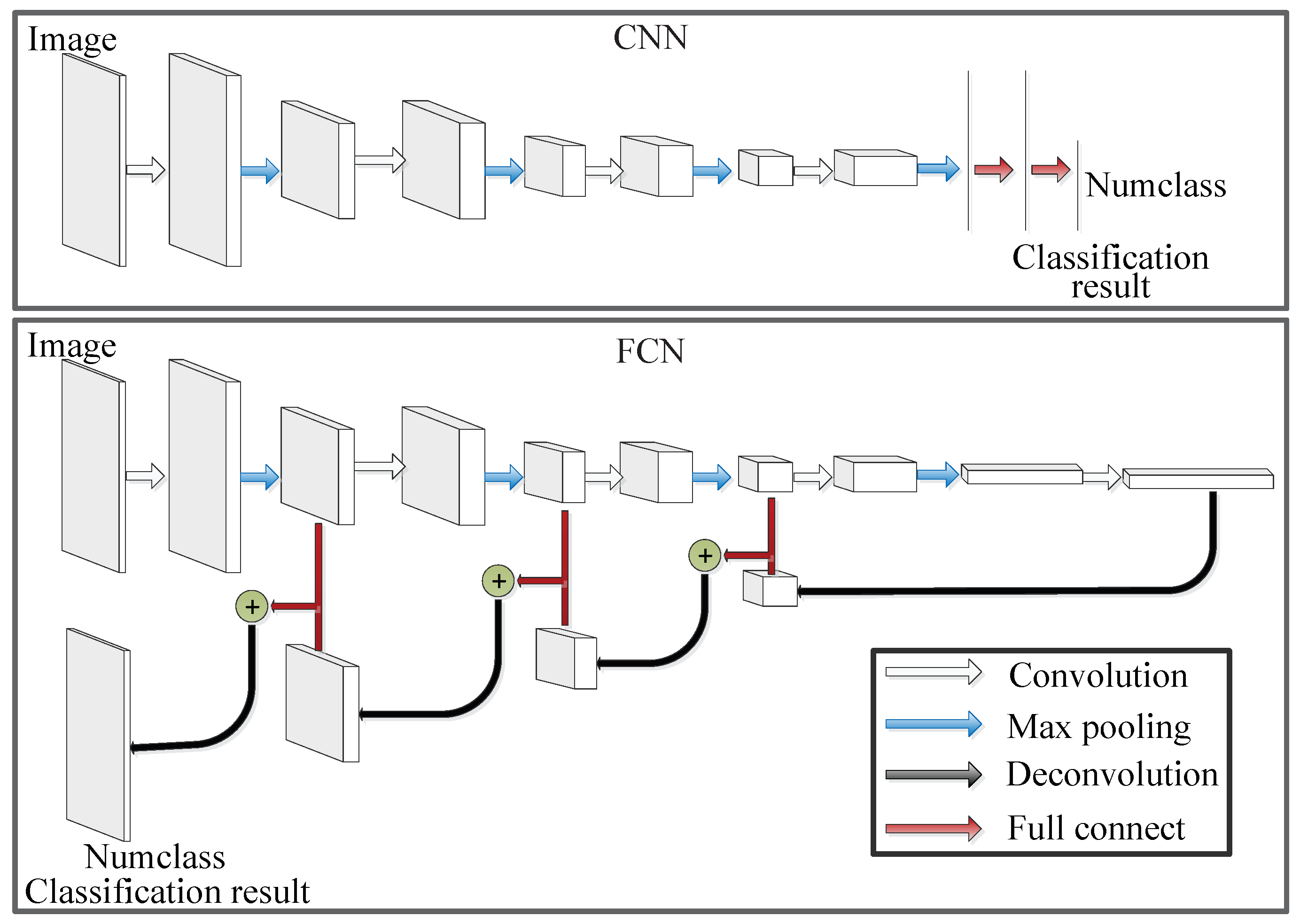
Fortunately, Long et al. [44] put forward Fully Convolutional Network (FCN) model, which is shown in Figure 1 and can be trained end-to-end, pixels-to-pixels. FCN transforms fully connected layers into convolutional layers, which enables an efficient classification net for end-to-end dense learning. That is to say, FCN is a promising method in PolSAR image classification. However, to utilize FCN for PolSAR image classification, some problems need to be solved, which can be described as follows:
- (1)
- As for common PolSAR image classification architectures, only a portion of labeled pixels are selected for training. However, for the FCN architecture, the whole ground truth map is used in the training stage;
- (2)
- As for the FCN architecture, each pixel in the images must have a corresponding label in the ground truth maps. However, there are some unlabeled pixels in the ground truth maps of the PolSAR images because PolSAR images are generally not fully labeled;
- (3)
- In general, each PolSAR image is trained individually, and the size of each PolSAR image is different. However, we cannot design an architecture for each image alone. Furthermore, a larger-size input image usually means a more complex architecture.
Recently, Wang et al. [45] have applied FCN to PolSAR image classification. However, they did not give the details of how to solve the problems mentioned. In order to provide a general solution to the problems aforementioned above, we propose sliding window fully convolutional network (SFCN). The sliding window operation of SFCN is similar to the sliding window operation of CNN, and the images obtained by sliding window operation are called as in this paper. As for SFCN, there are some details to state. First, the region where sliding window passes is extracted as directly, without convolution operation. In addition, the obtained is set as the input of FCN. Second, the size of the window is also the size of ; therefore, we can design a network architecture for all PolSAR images. Finally, because the training framework of FCN cannot be applied directly, we have designed a new training framework for SFCN in this paper.
However, the number of will increase with the increase of the image size, which leads to heavier computation burden and more memory occupation. Since sparse coding can better model the complex local image structures and it has achieved many promising results in PolSAR image classification [18,46,47], we think sparse coding can be utilized to model the local structures of PolSAR image. In this way, PolSAR image can be downsampled to a smaller size, so that the number of the can be limited. Therefore, finding a suitable sparse coding method becomes the key to the problem. Lately, Chen et al. [46] proposed multi-layer projective dictionary pair learning (MDPL), which can be used here to deal with the problem above without obvious image information loss.
Based on SFCN and sparse coding, we propose sliding window fully convolutional network and sparse coding (SFCN-SC) for PolSAR image classification, which can obtain excellent classification results while reducing the computational burden and memory occupation. The remainder of this paper is structured as follows: Section 2 gives the methods used for extracting features of PolSAR images. Our proposed method is presented in Section 3. Section 4 gives the experimental results. Finally, discussion and conclusions are given in Section 5 and Section 6, respectively.
2. Feature Extraction of PolSAR Images
2.1. Coherency Matrix
According to [48], each pixel in PolSAR image can be described by a scattering matrix, which contains the polarimetric information of the PolSAR data. With linear horizontal (H) and vertical (V) polarizations for transmitting and receiving, the scattering matrix can be formulated as:
where the reciprocity theorem applies in a mono-static system configuration results = , the scattering matrix can be described as [49]:
where
In addition, the coherency matrix of PolSAR data can be described as [48]:
2.2. Cloude–Pottier Decomposition
According to the eigen-decomposition model [11], the coherence matrix can be decomposed as:
where represents the eigenvector matrix of the coherency matrix T, and represents the eigenvalue of the coherency matrix . Based on the eigen-decomposition model, Cloude and Pottier proposed the Cloude–Pottier decomposition method, in which the entropy H, the anisotropy A, and the mean alpha angle can be obtained as:
where represents the first element of the eigenvector (i = 1, 2, 3). In addition, the Cloude–Pottier decomposition features have also been successfully used in PolSAR image classification [11,18].
In this paper, we utilize the coherency matrix T (, , , Re(), Re(), Re(), Im(), Im(), Im(), where Re() and Im() represent the real part and the imaginary part of respectively, and the Cloude–Pottier decomposition features (H, A, , , , ) to construct our extracted features.
3. Methodology
As for the traditional CNN architecture [50], the convolutional layers are used for extracting local features of images, and the fully connected layers are used for predicting the labels of images. In other words, the traditional CNN architecture cannot be trained pixels-to-pixels, which means that the classification results of CNN cannot reflect the labels of all the piexls in the images. However, the task of PolSAR image classification is to make a prediction at each pixel. Therefore, the pixels-to-pixels architecture is more suitable for processing PolSAR image classification task than CNN. Fortunately, Long et al. [44] proposed FCN model, which can be trained end-to-end, pixels-to-pixels. Therefore, FCN has enormous potential in PolSAR image classification.
Because of the advantages of the FCN model, we wish to utilize the FCN model for PolSAR image classification. However, some necessary improvements to the FCN model have to be done according to the problems as described in Section 1. In general, supervised methods used for PolSAR image classification usually select a portion of the labeled pixels as the training data and the remaining labeled pixels as the testing data, but, for the FCN architecture, the whole ground truth map of a certain image will participate in the training stage and all pixels in the image must have their own corresponding labels in the ground truth map. It is difficult to use FCN for classifying the PolSAR images, of which there are some unlabeled pixels in the ground truth maps, because most of the PolSAR images are not fully labeled. Therefore, the training framework of FCN [44] cannot be applied directly for PolSAR image classification. According to this, a new training framework of FCN is redesigned. Furthermore, images of different sizes need different FCN architectures and a larger-size input image usually brings more difficulty in designing network architecture. To design a unified FCN model for different images, a sliding window operator is introduced in this paper. Overall, a method named sliding window fully convolutional network (SFCN) is proposed to tackle the problems referred to above.
The sliding window operation of SFCN is similar to the sliding window operation of CNN, and the number of the can be obtained through
where ceil represents the upward integer-valued function, Height and Width represent the height and width of the input image, respectively, W is the size of the sliding window, S represents the stride of the sliding window operation, and Num represents the number of the . The obtained is set as the input of FCN. The advantages of SFCN can be described as follows:
- (1)
- SFCN can avoid repeated calculation and memory occupation which exist in CNN;
- (2)
- Supposing that there are three categories in the image, then these sliding window images may contain one, two, or three categories. Compared with the whole image being set as the input, we think the sliding window operation makes SFCN more constructive to learn the difference between different categories in ;
- (3)
- obtained by SFCN can contain more spatial information since the size of sliding window for SFCN is larger than that of CNN;
- (4)
- For SFCN with overlapping sliding window, there are multiple windows passing through almost all the pixels of the images except the edge parts, and each will give its own predicted results of the pixels. Combining multiple classification results can make the final result more reasonable.
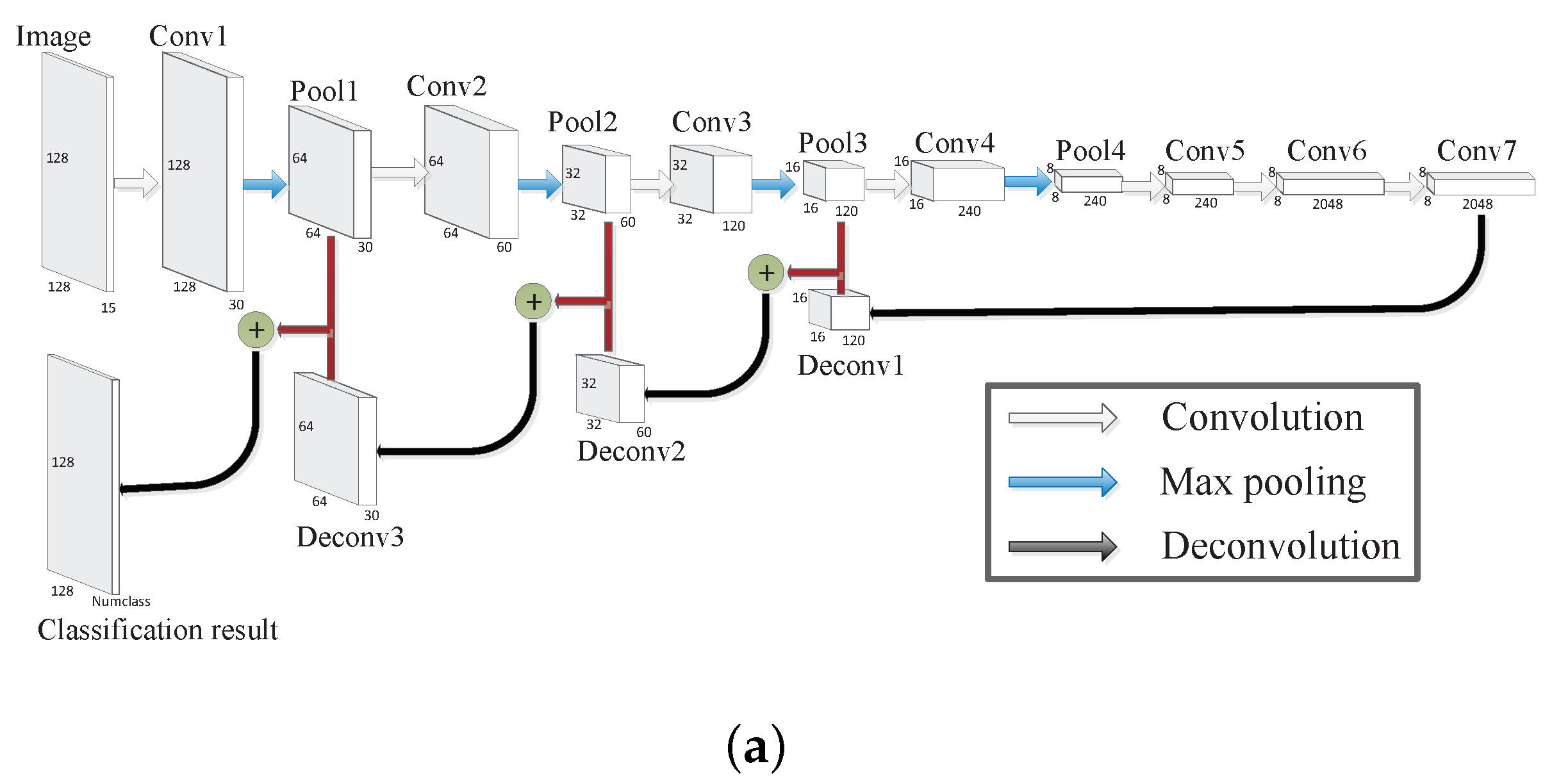
The architecture of the SFCN is shown in Figure 2. From Figure 2, we can see that two architectures, namely SFCN-128 and SFCN-256, have been designed for FCN in this paper. In addition, the loss function can be described as:
where y and represent the ground truth and the predicted result of , respectively, N represents the number of training samples in , and Numclass represents the classes number of .
Furthermore, there are some details to describe for the new training framework for SFCN. First, the training pixels are randomly selected. Second, only the training samples are involved in modifying the network parameters. The new training framework for SFCN is shown in Algorithm 1.
| Algorithm 1 The training framework of SFCN. |
| Input: Images , ground truth , training samples ratio ; 1: Initialize model parameters ; 2: Randomly select training samples from labeled samples, and the samples ratio of each class is p; 3: Utilize sliding window operation to get the sliding window image, recorded as ; 4: Initialize a zero matrix as the ground truth of each ; 5: if the pixel in is selected as training data then 6: Get the label of the pixel according to , recorded as L; 7: Set the element in g corresponding to the pixel to L; 8: end if 9: Set and as the input of SFCN; 10: Utilize ADAM [51] algorithm to minimize the loss function of SFCN, namely Equation (8), and only the non-zero points in are involved in model parameter updating. Output: SFCN learnt parameters: . |
According to Equation (7), the Num will increase with the increase of Height and Width under the condition that W and S are fixed. A larger number of will bring heavier computational burden and more memory occupation. As Section 1 described, sparse coding can be utilized to model the local structures of PolSAR image. Through sparse coding, PolSAR image can be downsampled to a smaller size. In this way, the number of the can be limited. Thus, the recently proposed MDPL model, as one of the sparse coding methods, is chosen to accomplish the downsampling task. MDPL model can be formulated as:
where represents the input data of the lth layer, represents the coding coefficients of the lth layer, { and } represents the projective dictionary pair of the lth layer, represents a scalar constant, and is the ith atom of . In addition, is set as the input of the first layer, and the coding coefficients of the previous layer are set as the input of the next layer. Because MDPL belongs to the sparse coding methods, MDPL can tackle the downsampling task while maintaining the image integrity to the maximum extent.
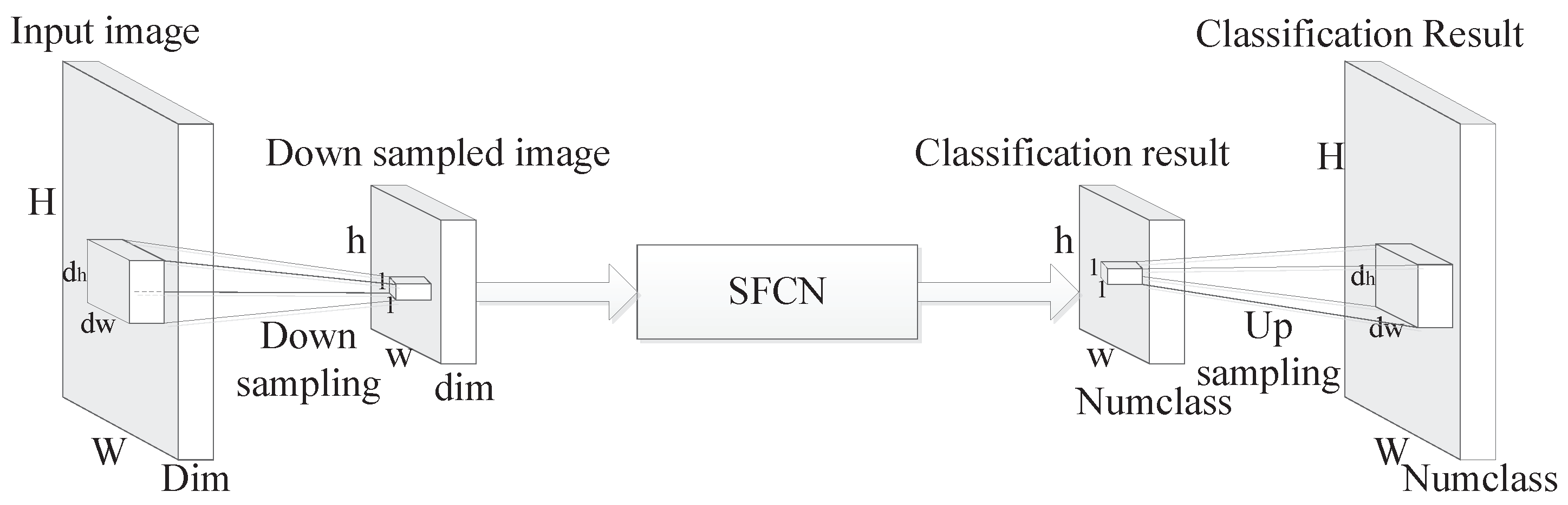
Based on SFCN and sparse coding, we propose sliding window fully convolutional network and sparse coding (SFCN-SC) in this paper. There are some details to state for SFCN-SC. First, the input image (recorded as ) is cut into small blocks, and the features of each small block are flattened into a feature vector, recorded as . Then, is set as the input of MDPL to obtain the coding coefficients, recorded as . In this way, the input image is downsampled to a smaller size, recorded as . In other words, each pixel in has a corresponding small block in . Second, is set as the input of SFCN to obtain the classification result of , recorded as , and the size of is the same as that of , not the same as . Third, the element of is set as the classification result of the corresponding small block to obtain the final classification result. The algorithm architecture of SFCN-SC is shown in Figure 3, and the implementation details of SFCN-SC are described in Algorithm 2.
| Algorithm 2 The framework of SFCN-SC. |
| Input: Images , ground truth , training samples ratio , the size of small block × , the size of the extracted feature through MDPL dim; 1: Get the feature dimension of , recorded as Dim; 2: Cut the image into small blocks, and the size of the small blocks is × ; 3: Flat all the features of each small block into feature vector, recorded as , and the dimension of is ·· Dim; 4: Set and as the input of MDPL, get the coding coefficients ; 5: Each small block operates 3–4, in this way, is downsampled to a smaller size, recorded as , which is the downsampled image; 6: Set the popular label of the pixels in each small block as the label of , recorded as , each small block operates this to obtain the ground truth of , recorded as ; 7: Set , and as the input of SFCN to get the classification result through Algorithm 1, recorded as ; 8: Set the element of as the classification result of the corresponding small block in X to obtain the final classification result of the X, recorded as Result. Output: Classification result Result. |
4. Experimental Results
As described in Section 2, the coherency matrix T (, , , Re(), Re(), Re(), Im(), Im(), Im() and the Cloude–Pottier decomposition features (H, A, , , , ) are set as our input features in this paper. The refined Lee filter [52] is used for suppressing the speckle noise. Three PolSAR images, including images for Xi’an, China; Oberpfaffenhofen, Germany; San Francisco, CA, USA are utilized to test the performances of different methods. In addition, Table 1 gives the detail information of the three PolSAR images. We utilize overall accuracy (OA) and Kappa coefficient [53] to evaluate the performances of different methods. In the following experiments, SVM [20], sparse representation classifier (SRC) [54], CNN [55] and SAE [30] are used as the compared methods. In this paper, all methods (including our method and compared methods) are implemented in a 2.20-GHz machine with a 64.00-GB RAM and a NVIDIA GTX 1080 GPU.
4.1. Parameter Setting
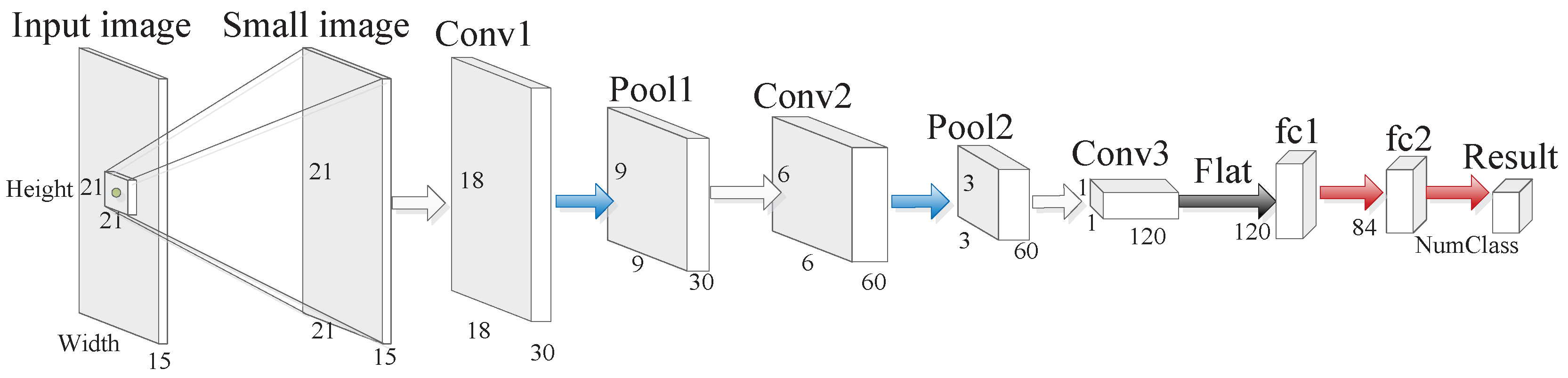
For the SVM method, the radial basis function (RBF) kernel is used. As for the SRC, the number of dictionary atoms is set to 15. For the CNN method, we use a neighborhood of each pixel as the small image, and the architecture of CNN is shown in Figure 4. As for SAE, the dimensions of middle layers are 300 and 100, respectively, and Softmax classifier [56] is utilized to get the classification result. As to our proposed method SFCN, we design two architectures, namely SFCN-128 and SFCN-256, which are shown in Figure 2. For the SFCN-SC method, which is shown in Figure 3, we downsample Oberpfaffenhofen and San Francisco to and , recorded as , and the dimension of the pixel in is set to 10. Then, is set as the input of SFCN. We set stride in Equation (7) to 32 and 64 for the window images of 128 and 256 sizes, respectively. In the following experiments, the number of training samples of each class corresponding to all the three PolSAR images is 5%, and the training samples are randomly selected.
4.2. Classification Performance
4.2.1. Xi’an Image
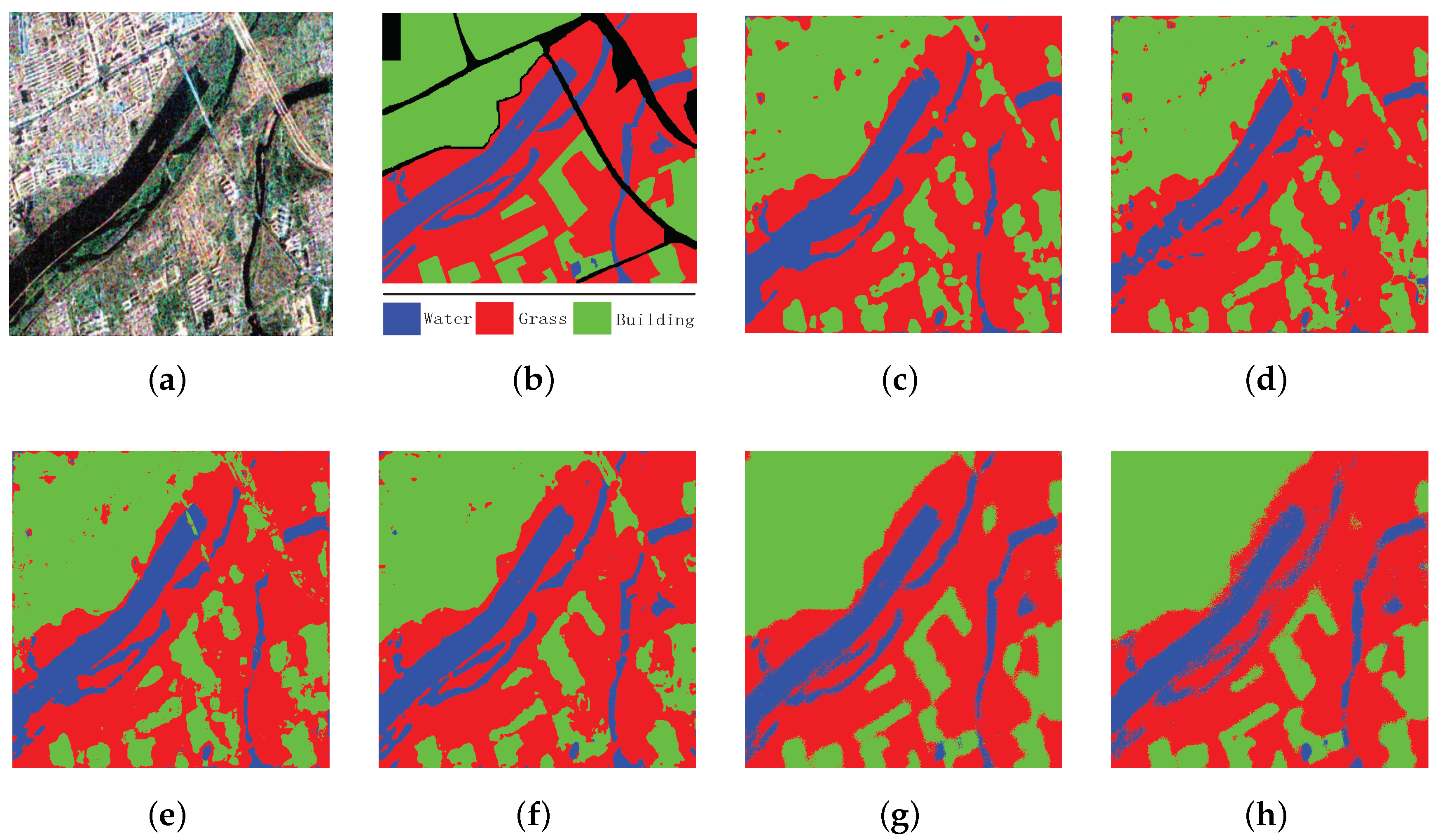
Figure 5a,b give the Pauli RGB (red-green-blue) image and the ground truth of Xi’an, respectively. There are 237,416 labeled pixels in the ground truth. As Section 4.1 mentioned, we use 5% of the labeled pixels in the ground truth as the training set and the remaining 95% as the testing set. Figure 5c–h and Table 2 give the classification results, which can be utilized to compare the performances of different methods.
From Figure 5, we can see that the classification result of SFCN-128 is more reasonable than other methods. The classification results of SVM, SRC and SAE are relatively worse, because there are many misclassified pixels in Figure 5c–e. From Table 2, we can get the same conclusion. The accuracy values and Kappa coefficient of SFCN-128 are the highest among all the methods, and accuracy values and Kappa coefficient of SRC are the lowest. For that mentioned above, the effectiveness of our method can be verified.
4.2.2. Oberpfaffenhofen Image
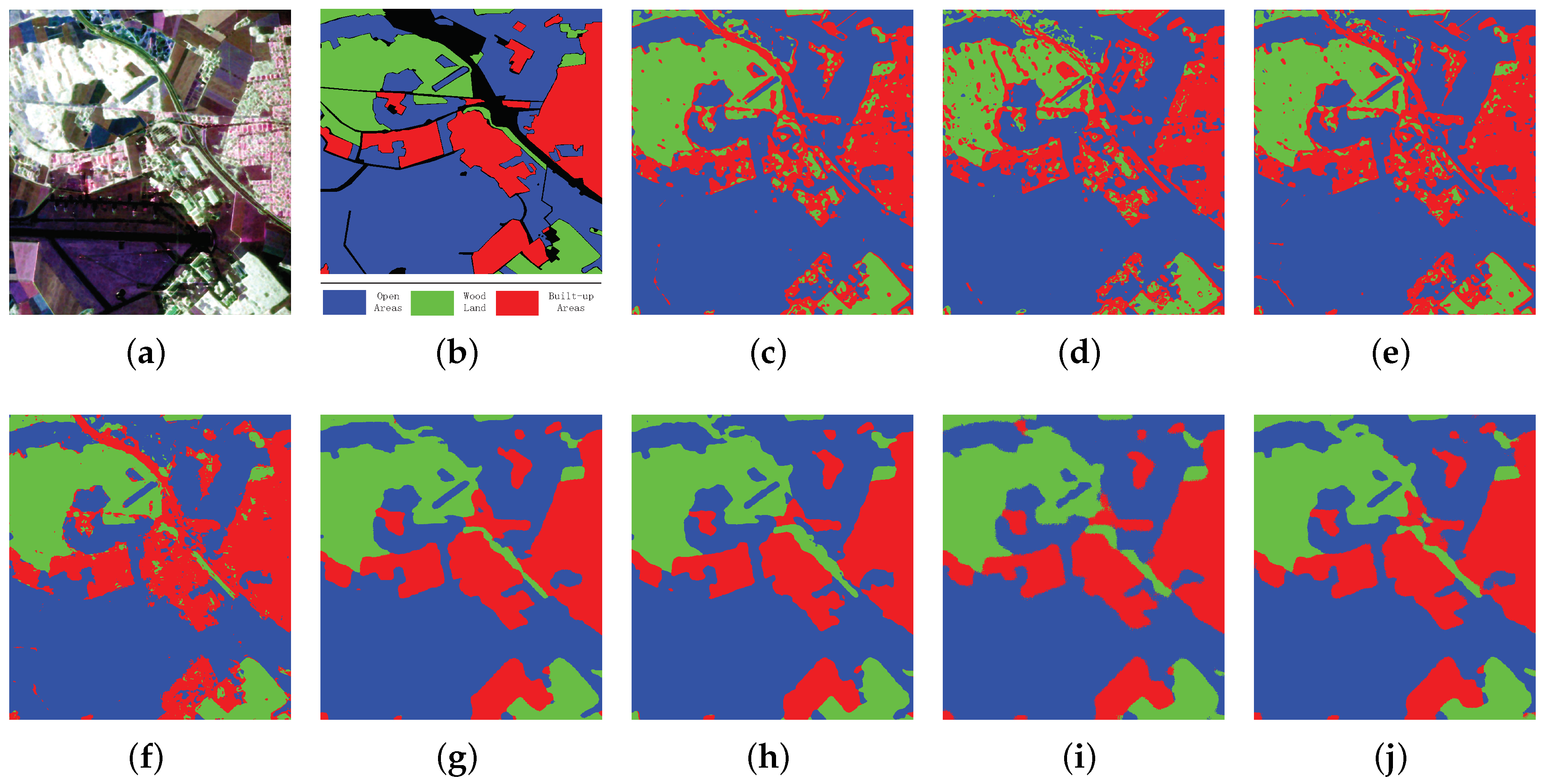
Figure 6a,b gives the Pauli RGB image and the ground truth of Oberpfaffenhofen, respectively. There are 1,374,298 labeled pixels in the ground truth. Just as Section 4.1 mentioned, 5% of the labeled pixels in the ground truth are set as the training set and the remaining 95% are set as the testing set. Figure 6c–j and Table 3 show the classification results to compare the effectiveness of different methods.
As shown in Figure 6, the number of the misclassified pixels corresponding to SFCN-128 and SFCN-256 is smaller than other methods, which can demonstrate the effectiveness of SFCN. As to SFCN-SC (including SFCN-SC-128 and SFCN-SC-256), the classification results are comparable to SFCN. In agreement with Xi’an image, the classification results corresponding to SVM, SRC and SAE are relatively worse than other methods. We can get the same conclusion from Table 3. As shown in Table 3, the accuracy values and Kappa coefficient of SFCN are the highest among all the methods, and the accuracy values and Kappa coefficient of SFCN-SC are a little lower than but comparable to SFCN. Therefore, we can draw a conclusion that our sparse coding method can maintain the image integrity to the maximum while accomplishing the downsampling task. In summary, the effectiveness of our method can be made evident by the reasons mentioned above.
4.2.3. San Francisco Image
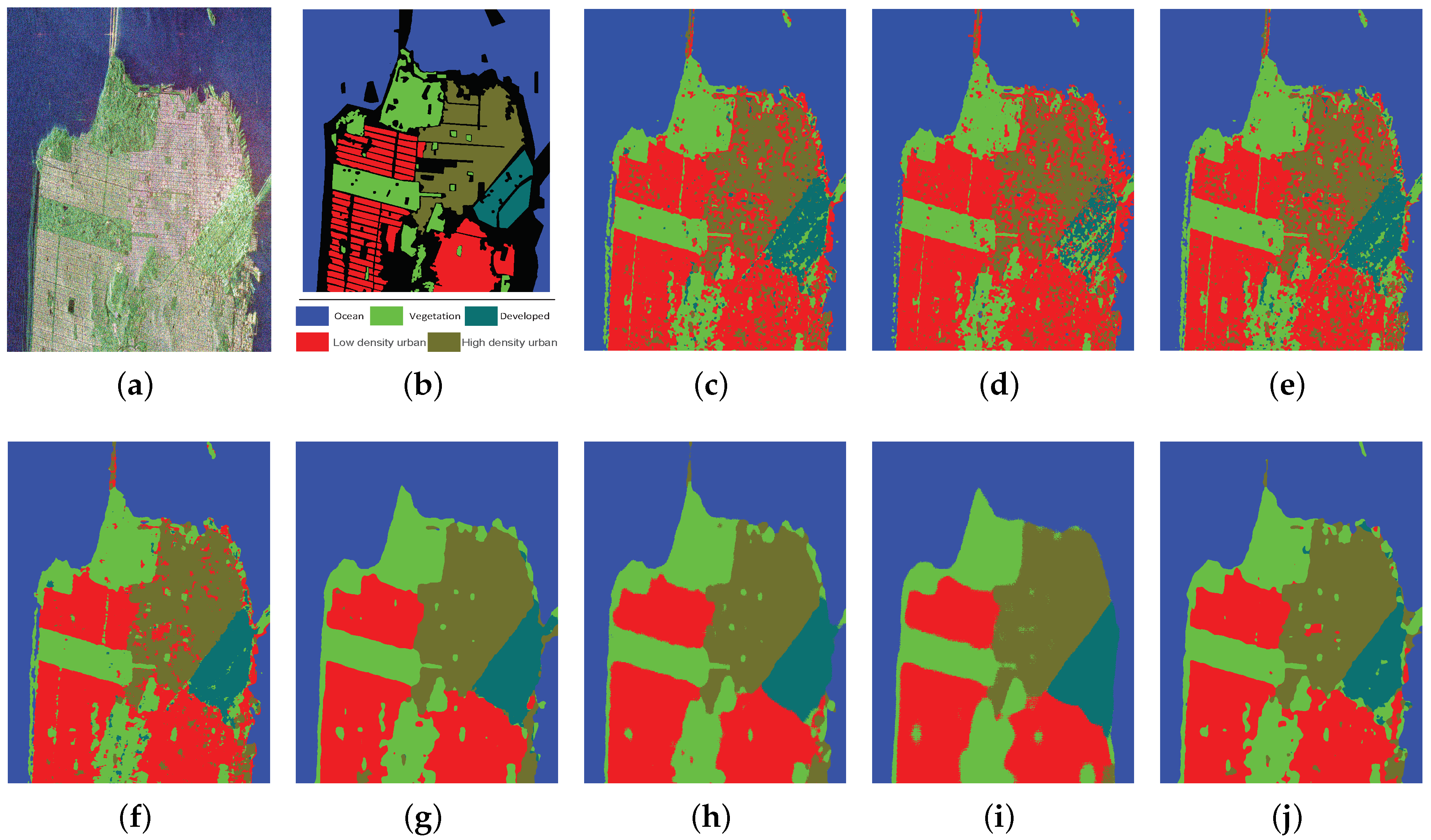
Figure 7a,b shows the Pauli RGB image and the ground truth of San Francisco, respectively. The number of labeled pixels in the ground truth is 1,804,087. Just as Section 4.1 said, 5% of the labeled pixels in the ground truth are invoked as the training set and the remaining 95% are used as the testing set. Figure 7c–j and Table 4 show the classification results of all the methods. The classification results of San Francisco image are similar to the two above mentioned images. SFCN obtains the best classification results among all the methods, and the classification results of SFCN-SC are comparable to SFCN. The classification results corresponding to SVM, SRC and SAE are relatively worse. For that mentioned above, the effectiveness of our method can be proved.
5. Discussion
5.1. The Comparison of Performance of Architectures with Different Window Sizes
In this paper, two window sizes are adopted, namely 128 and 256. It can be seen from Table 2, Table 3 and Table 4 that the classification results corresponding to 128 are usually better than or comparable to that corresponding to 256. However, the network architecture using the 128 size of window has lower complexity compared to the other one. Therefore, 128 is a more ideal window size for SFCN and SFCN-SC.
5.2. The Effect of Sliding Window on the Classification Results
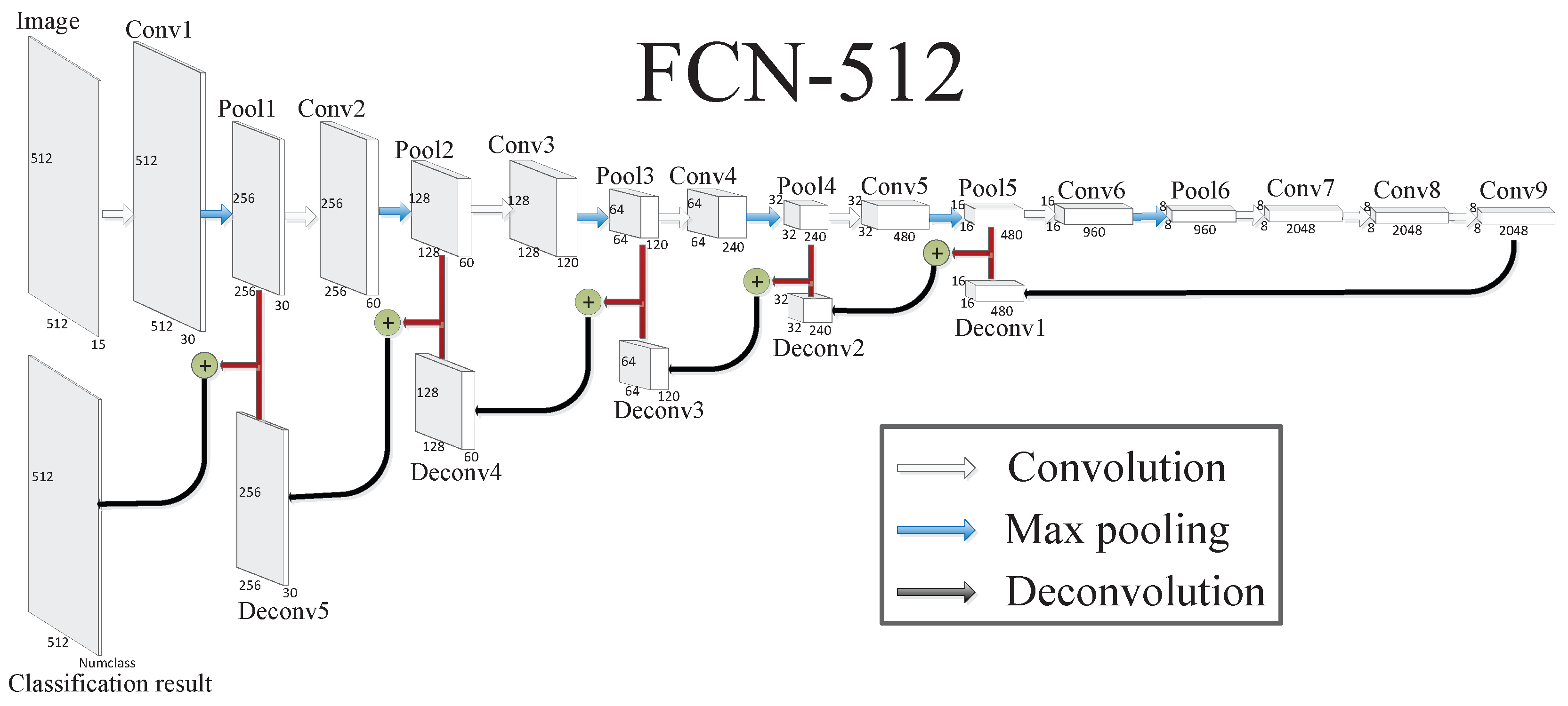
There are three PolSAR images in this paper, including Xi’an, Oberpfaffenhofen, and San Francisco, and the sizes of the three PolSAR images are , , and , respectively. The FCN architectures for Oberpfaffenhofen and San Francisco are too hard to design because of their larger image sizes. Therefore, as shown in Figure 8, we design a FCN architecture for Xi’an as the contrast method of SFCN-128 and SFCN-256, namely FCN-512, to validate the effect of sliding window on the classification results.
Table 5 shows the classification results of Xi’an with FCN-512, SFCN-128 and SFCN-256 as a function of the rate of training samples. It can be seen that the OA of FCN-512 is 0.9634, a little smaller than that of SFCN-128 and SFCN-256, under 20% of training samples. When the rate of training samples decrease from 20% to 5%, the OA of FCN-512 falls sharply to 0.6372 but the OA of SFCN-128 and SFCN-256 remain over 0.93. Therefore, SFCN can obtain better classification results even using less training samples compared to FCN-512, which proves that the sliding window is useful to improve the classification results.
5.3. The Effect of Sparse Coding
As presented in Section 3, the number of the sliding window images obtained by SFCN will increase with the image size, which increases the computational burden in the training stage. In this paper, we use sparse coding to resolve this problem. As two of the most popular downsampling methods, the bilinear interpolation (BILI) [57] and bicubic interpolation (BICI) [58] methods have achieved great performance in image processing in the past decades. Therefore, BILI and BICI are used to compare the performance of sparse coding. In addition, the compared methods are recorded as SFCN-BILI and SFCN-BICI. Table 6 gives the classification results of Oberpfaffenhofen and San Francisco with SFCN, SFCN-BILI, SFCN-BICI, and SFCN-SC. We can see that the classification results of SFCN-BILI and SFCN-BICI are much lower than SFCN. However, the classification results of SFCN-SC are a little lower than but comparable to SFCN. Based on the above discussion, we can draw a conclusion that the popular downsampling method, such as BILI and BICI, may result in the loss of details of the PolSAR image, but sparse coding can maintain the details of the PolSAR image in the maximum extent. Table 7 summarizes the execution time of various methods, where “Train” represents the training time, “Predict” represents the time taken to classify entire image, and “Total” represents the total time taken to train plus predict. The training time consumption of SFCN-SC can be divided into two parts, namely SFCN and sparse coding. Though sparse coding consumes a certain amount of time at the training stage, the training time of SFCN-SC is less than SFCN. In summary, SFCN-SC still can obtain competitive classification results while reducing the computational burden in the training stage.
5.4. Data Memory Consumed by Various Methods
Table 8 gives the data memory consumed by various methods corresponding to the three PolSAR images, and the “G” in the caption of Table 8 represents gigabytes. From Table 8, we can see that the data memory consumed by CNN is the highest among all the methods, which demonstrates that CNN does have the disadvantage of repeated memory occupation. The data memory consumed by SFCN-SC is smaller than SFCN, since the data memory occupation can be reduced by sparse coding. In summary, SFCN-SC does have an advantage over CNN and SFCN in memory occupation. black
To sum up, the classification results of SVM, SRC and SAE are relatively worse because these three methods cannot take into account the spatial information of the images. However, they are superior to other methods in memory occupation. As for the time consumption, SRC and SAE performs well. Nonetheless, in order to fit the relationship between the training data and the training label, SVM has caused its structure to be too complicated. Therefore, SVM takes a relatively longer time to predict the images. The neighborhood of the pixel is used as the input of CNN, and in this way the spatial information can be used by CNN. Therefore, the classification result of CNN is acceptable. However, setting the neighborhoods of the pixels as the input of CNN also leads to repeated calculation and memory occupation, which means that CNN has no advantage over other methods in terms of time consumption and memory occupation. As Section 1 described, PolSAR image classification is actually a dense prediction problem, and FCN does have great potential in PolSAR image classification because of its special network architecture. However, the traditional FCN architecture cannot be applied directly to PolSAR image classification. Based on FCN, we utilize sliding window operation to tackle the problem. From the classification results of the three PolSAR images, we can note that the classification results of SFCN are better than CNN and SAE. This is because SFCN takes the spatial information into account and the spatial information of SFCN is more abundant than that of CNN. However, the sliding window operation also increases computational burden and memory occupation. Thus, we utilize sparse coding as the downsampling method to reduce the num of . In addition, classification results will hardly be affected because sparse coding can find the key information of the image. In summary, SFCN-SC is the only algorithm that can take into account the classification results, time consumption, and memory occupation at the same time.
6. Conclusions
In this paper, we propose a novel method, namely SFCN-SC, for PolSAR image classification. The coherency matrix T and Cloude–Pottier decomposition features are used as the feature vectors, SVM, SRC, SAE and CNN are utilized as the compared methods, and three PolSAR images, including Xi’an, Oberpfaffenhofen, and San Francisco are used to test the performances of different methods. On the basis of the previous FCN model and sliding window operation, we propose SFCN to obtain more competitive classification results. However, time consumption and memory occupation of SFCN will increase with the increase of the image size. In order to address the problem mentioned above, sparse coding is used as the downsampling method in our method. We first downsample the images to a fixed size, and the obtained images through downsampling are set as the input of SFCN. In this way, the time consumption and memory occupation can be reduced. Because of the great performances of SFCN and sparse coding, SFCN-SC can get competitive classification results while reducing the time consumption and memory occupation. Compared with some state-of-the-art methods, SFCN-SC achieves impressive performance in PolSAR image classification.
Author Contributions
Methodology, Y.L. and Y.C.; Resources, L.J.; Software, G.L.; Writing review & editing, Y.C.
Funding
This work was supported in part by the project supported the Foundation for Innovative Research Groups of the National Natural Science Foundation of China under Grant 61621005, in part by the National Natural Science Foundation of China under Grant 61772399, Grant U1701267, Grant 61773304, and Grant 61772400, and in part by the Technology Foundation for Selected Overseas Chinese Scholar in Shaanxi under Grant 2017021 and Grant 2018021.
Acknowledgments
The authors would like to thank all reviewers and editors for their comments on this paper.
Conflicts of Interest
The authors declare no conflicts of interest.
Abbreviations
The following abbreviations are used in this manuscript:
| PolSAR | Polarimetric synthetic aperture radar |
| FCN | Fully convolutional network |
| SFCN | Sliding window fully convolutional network |
| SFCN-SC | Sliding window fully convolutional network and sparse coding |
| CNN | Convolutional neural network |
| KNN | K-nearest neighbor |
| SVM | Support vector machine |
| SAE | Stacked auto-encoder |
| DBN | Deep belief network |
| MDPL | Multi-layer projective dictionary pair learning |
| OA | Overall accuracy |
| SRC | Sparse representation classifier |
| RBF | Radial basis function |
| RGB | Red-green-blue |
| BILI | Bilinear interpolation |
| BICI | Bicubic interpolation |
References
- Zhang, L.; Chen, Y.; Lu, D.; Zou, B. Polarmetric SAR images classification based on sparse representation theory. In Proceedings of the IEEE International Geoscience and Remote Sensing Symposium (IGARSS), Melbourne, Australia, 21–26 July 2013; pp. 3179–3182. [Google Scholar]
- Chen, W.; Gou, S.; Wang, X.; Li, X.; Jiao, L. Classification of PolSAR Images Using Multilayer Autoencoders and a Self-Paced Learning Approach. Remote Sens. 2018, 10, 110. [Google Scholar] [CrossRef]
- Zhang, F.; Ni, J.; Yin, Q.; Li, W.; Li, Z.; Liu, Y.; Hong, W. Nearest-Regularized Subspace Classification for PolSAR Imagery Using Polarimetric Feature Vector and Spatial Information. Remote Sens. 2017, 9, 1114. [Google Scholar] [CrossRef]
- Hou, B.; Chen, C.; Liu, X.; Jiao, L. Multilevel distribution coding model-based dictionary learning for PolSAR image classification. IEEE J. Sel. Top. Appl. Earth Obs. Remote Sens. 2015, 8, 5262–5280. [Google Scholar]
- Cheng, J.; Ji, Y.; Liu, H. Segmentation-based PolSAR image classification using visual features: RHLBP and color features. Remote Sens. 2015, 7, 6079–6106. [Google Scholar] [CrossRef]
- Tao, C.; Chen, S.; Li, Y.; Xiao, S. PolSAR land cover classification based on roll-invariant and selected hidden polarimetric features in the rotation domain. Remote Sens. 2017, 9, 660. [Google Scholar]
- Xu, Q.; Chen, Q.; Yang, S.; Liu, X. Superpixel-based classification using K distribution and spatial context for polarimetric SAR images. Remote Sens. 2016, 8, 619. [Google Scholar] [CrossRef]
- Krogager, E. New decomposition of the radar target scattering matrix. Electron. Lett. 1990, 26, 1525–1527. [Google Scholar] [CrossRef]
- Freeman, A.; Durden, S.L. A three-component scattering model for polarimetric SAR data. IEEE Trans. Geosci. Remote Sens. 1998, 36, 963–973. [Google Scholar] [CrossRef]
- Huynen, J.R. Phenomenological theory of radar targets. Electromagn. Scatt. 1978, 653–712. [Google Scholar] [CrossRef]
- Cloude, S.R.; Pottier, E. An entropy based classification scheme for land applications of polarimetric SAR. IEEE Trans. Geosci. Remote Sens. 1997, 35, 68–78. [Google Scholar] [CrossRef]
- Van Zyl, J.J.; Arii, M.; Kim, Y. Model-based decomposition of polarimetric SAR covariance matrices constrained for nonnegative eigenvalues. IEEE Trans. Geosci. Remote Sens. 2011, 49, 3452–3459. [Google Scholar] [CrossRef]
- Yamaguchi, Y.; Moriyama, T.; Ishido, M.; Yamada, H. Four-component scattering model for polarimetric SAR image decomposition. IEEE Trans. Geosci. Remote Sens. 2005, 43, 1699–1706. [Google Scholar] [CrossRef]
- Kong, J.A.; Swartz, A.A.; Yueh, H.A.; Novak, L.M.; Shin, R.T. Identification of terrain cover using the optimum polarimetric classifier. J. Electromagn. Waves Appl. 1988, 2, 171–194. [Google Scholar]
- Lee, J.-S.; Grunes, M.R.; Kwok, R. Classification of multi-look polarimetric SAR imagery based on complex Wishart distribution. Int. J. Remote Sens. 1994, 15, 2299–2311. [Google Scholar] [CrossRef]
- Lee, J.-S.; Grunes, M.R.; Ainsworth, T.L.; Du, L.-J.; Schuler, D.-L.; Cloude, S.R. Unsupervised classification using polarimetric decomposition and the complex Wishart classifier. IEEE Trans. Geosci. Remote Sens. 1999, 37, 2249–2258. [Google Scholar]
- Richardson, A.; Goodenough, D.G.; Chen, H.; Moa, B.; Hobart, G.; Myrvold, W. Unsupervised nonparametric classification of polarimetric SAR data using the K-nearest neighbor graph. In Proceedings of the IEEE International Geoscience and Remote Sensing Symposium (IGARSS), Honolulu, HI, USA, 25–30 July 2010; pp. 1867–1870. [Google Scholar]
- Zhang, L.; Sun, L.; Zou, B.; Moon, W.M. Fully Polarimetric SAR Image Classification via Sparse Representation and Polarimetric Features. IEEE J. Sel. Top. Appl. Earth Obs. Remote Sens. 2015, 8, 3923–3932. [Google Scholar] [CrossRef]
- Zhang, L.; Zou, B.; Zhang, J.; Zhang, Y. Classification of polarimetric SAR image based on support vector machine using multiple-component scattering model and texture features. EURASIP J. Adv. Signal Process. 2010. [Google Scholar] [CrossRef]
- Lardeux, C.; Frison, P.L.; Tison, C.C.; Souyris, J.C.; Stoll, B.; Fruneau, B.; Rudant, J.P. Support vector machine for multifrequency SAR polarimetric data classification. IEEE Trans. Geosci. Remote Sens. 2009, 47, 4143–4152. [Google Scholar] [CrossRef]
- Fukuda, S.; Hirosawa, H. Support vector machine classification of land cover: Application to polarimetric SAR data. In Proceedings of the IEEE International Geoscience and Remote Sensing Symposium (IGARSS), Sydney, Australia, 9–13 July 2001; pp. 187–189. [Google Scholar]
- Yueh, H.A.; Swartz, A.A.; Kong, J.A.; Shin, R.T.; Novak, L.M. Bayes classification of terrain cover using normalized polarimetric data. J. Geophys. Res. 1988, 93, 15261–15267. [Google Scholar] [CrossRef]
- Chen, K.-S.; Huang, W.; Tsay, D.; Amar, F. Classification of multifrequency polarimetric SAR imagery using a dynamic learning neural network. IEEE Trans. Geosci. Remote Sens. 1996, 34, 814–820. [Google Scholar] [CrossRef]
- Hellmann, M.; Jager, G.; Kratzschmar, E.; Habermeyer, M. Classification of full polarimetric SAR-data using artificial neural networks and fuzzy algorithms. In Proceedings of the IEEE International Geoscience and Remote Sensing Symposium (IGARSS), Hamburg, Gemany, 28 June–2 July 1999; pp. 1995–1997. [Google Scholar]
- Chen, C.; Chen, K.; Lee, J. The use of fully polarimetric information for the fuzzy neural classification of SAR images. IEEE Trans. Geosci. Remote Sens. 2003, 41, 2089–2100. [Google Scholar] [CrossRef]
- Dao, M.; Kwan, C.; Ayhan, B.; Tran, T.D. Burn scar detection using cloudy MODIS images via low-rank and sparsity-based models. In Proceedings of the 2016 IEEE Global Conference on Signal and Information Processing (GlobalSIP), Washington, DC, USA, 7–9 December 2016; pp. 177–181. [Google Scholar]
- Dao, M.; Kwan, C.; Koperski, K.; Marchisio, G. A joint sparsity approach to tunnel activity monitoring using high resolution satellite images. In Proceedings of the IEEE 8th Annual Ubiquitous Computing, Electronics & Mobile Communication Conference (UEMCON), New York, NY, USA, 19–21 October 2017; pp. 322–328. [Google Scholar]
- Chen, Y.; Nasrabadi, N.M.; Tran, T.D. Hyperspectral image classification using dictionary-based sparse representation. IEEE Trans. Geosci. Remote Sens. 2011, 49, 3973–3985. [Google Scholar] [CrossRef]
- Ayhan, B.; Dao, M.; Kwan, C.; Chen, H.; Bell, J.F.; Kidd, R. A Novel Utilization of Image Registration Techniques to Process Mastcam Images in Mars Rover With Applications to Image Fusion, Pixel Clustering, and Anomaly Detection. IEEE J. Sel. Top. Appl. Earth Obs. Remote Sens. 2017, 10, 4553–4564. [Google Scholar] [CrossRef]
- Xie, H.; Wang, S.; Liu, K.; Lin, S.; Hou, B. Multilayer feature learning for polarimetric synthetic radar data classification. In Proceedings of the IEEE International Geoscience and Remote Sensing Symposium (IGARSS), Quebec City, QC, Canada, 13–18 July 2014; pp. 2818–2821. [Google Scholar]
- Ayhan, B.; Kwan, C. Application of deep belief network to land cover classification using hyperspectral images. In Proceedings of the 14th International Symposium on Neural Networks (ISNN), Hokkaido, Japan, 21–23 June 2017; pp. 269–276. [Google Scholar]
- Krizhevsky, A.; Sutskever, I.; Hinton, G.E. Imagenet classification with deep convolutional neural networks. In Proceedings of the International Conference on Neural Information Processing Systems (NIPS), Lake Tahoe, NV, USA, 3–6 December 2012; pp. 1097–1105. [Google Scholar]
- Girshick, R.; Donahue, J.; Darrell, T.; Malik, J. Rich feature hierarchies for accurate object detection and semantic segmentation. In Proceedings of the IEEE Conference on Computer Vision and Pattern Recognition (CVPR), Columbus, OH, USA, 23–28 June 2014; pp. 580–587. [Google Scholar]
- Farabet, C.; Couprie, C.; Najman, L.; LeCun, Y. Learning hierarchical features for scene labeling. IEEE Trans. Pattern Anal. Mach. Intell. 2013, 35, 1915–1929. [Google Scholar] [CrossRef] [PubMed]
- Simonyan, K.; Zisserman, A. Two-stream convolutional networks for action recognition in videos. In Proceedings of the Conference on Advances in Neural Information Processing Systems (NIPS), Montreal, QC, Canada, 8–13 December 2014; pp. 568–576. [Google Scholar]
- Perez, D.; Banerjee, D.; Kwan, C.; Dao, M.; Shen, Y.; Koperski, K.; Marchisio, G.; Li, J. Deep learning for effective detection of excavated soil related to illegal tunnel activities. In Proceedings of the IEEE 8th Annual Ubiquitous Computing, Electronics & Mobile Communication Conference (UEMCON), New York, NY, USA, 19–21 October 2017; pp. 626–632. [Google Scholar]
- Lu, Y.; Perez, D.; Dao, M.; Kwan, C.; Li, J. Deep Learning with Synthetic Hyperspectral Images for Improved Soil Detection in Multispectral Imagery. In Proceedings of the IEEE 9th Annual Ubiquitous Computing, Electronics & Mobile Communication Conference (UEMCON), New York, NY, USA, 8–10 November 2018; pp. 8–10. [Google Scholar]
- Zhu, X.; Tuia, D.; Mou, L.; Xia, G.; Zhang, L.; Xu, F.; Fraundorfer, F. Deep Learning in Remote Sensing: A Comprehensive Review and List of Resources. IEEE Geosci. Remote Sens. Mag. 2017, 5, 8–36. [Google Scholar] [CrossRef] [Green Version]
- Zhou, Y.; Wang, H.; Xu, F.; Jin, Y. Polarimetric SAR image classification using deep convolutional neural networks. IEEE Geosci. Remote Sens. Lett. 2016, 13, 1935–1939. [Google Scholar] [CrossRef]
- Xie, W.; Jiao, L.; Hou, B.; Ma, W.; Zhao, J.; Zhang, S.; Liu, F. POLSAR image classification via Wishart-AE model or Wishart-CAE model. IEEE J. Sel. Top. Appl. Earth Obs. Remote Sens. 2017, 10, 3604–3615. [Google Scholar] [CrossRef]
- Chen, S.; Tao, C. PolSAR image classification using polarimetric-feature-driven deep convolutional neural network. IEEE Geosci. Remote Sens. Lett. 2018, 15, 627–631. [Google Scholar] [CrossRef]
- Wang, L.; Xu, X.; Dong, H.; Gui, R.; Pu, F. Multi-Pixel Simultaneous Classification of PolSAR Image Using Convolutional Neural Networks. Sensors 2018, 18, 769. [Google Scholar] [CrossRef]
- Chen, S.; Tao, C.; Wang, X.; Xiao, S. Polsar Target Classification Using Polarimetric-Feature-Driven Deep Convolutional Neural Network. In Proceedings of the IEEE International Geoscience and Remote Sensing Symposium (IGARSS), Valencia, Spain, 21–29 July 2018; pp. 4407–4410. [Google Scholar]
- Long, J.; Shelhamer, E.; Darrell, T. Fully convolutional networks for semantic segmentation. In Proceedings of the IEEE Conference on Computer Vision and Pattern Recognition (CVPR), Boston, MA, USA, 7–12 June 2015; pp. 3431–3440. [Google Scholar]
- Wang, Y.; He, C.; Liu, X.; Liao, M. A Hierarchical Fully Convolutional Network Integrated with Sparse and Low-Rank Subspace Representations for PolSAR Imagery Classification. Remote Sens. 2018, 10, 342. [Google Scholar] [CrossRef]
- Chen, Y.; Jiao, L.; Li, Y.; Zhao, J. Multilayer Projective Dictionary Pair Learning and Sparse Autoencoder for PolSAR Image Classification. IEEE Trans. Geosci. Remote Sens. 2017, 55, 6683–6694. [Google Scholar] [CrossRef]
- Hou, B.; Ren, B.; Ju, G.; Li, H.; Jiao, L.; Zhao, J. SAR image classification via hierarchical sparse representation and multisize patch features. IEEE Geosci. Remote Sens. Lett. 2016, 13, 33–37. [Google Scholar] [CrossRef]
- Liu, F.; Jiao, L.; Hou, B.; Yang, S. POL-SAR Image classification based on Wishart DBN and local spatia information. IEEE Trans. Geosci. Remote Sens. 2016, 54, 3292–3308. [Google Scholar] [CrossRef]
- Cloude, S.R.; Pottier, E. A review of target decomposition theorems in radar polarimetry. IEEE Trans. Geosci. Remote Sens. 1996, 34, 498–518. [Google Scholar] [CrossRef]
- Wang, Q.; Gao, J.; Yuan, Y. Embedding structured contour and location prior in siamesed fully convolutional networks for road detection. IEEE Trans. Intell. Transp. 2018, 19, 230–241. [Google Scholar] [CrossRef]
- Kingma, D.P.; Ba, J. Adam: A Method for Stochastic Optimization. In Proceedings of the International Conference on Learning Representations (ICLR), San Diego, CA, USA, 7–9 May 2015. [Google Scholar]
- Lee, J.-S.; Grunes, M.R.; De Grandi, G. Polarimetric SAR speckle filtering and its implication for classification. IEEE Trans. Geosci. Remote Sens. 1999, 37, 2363–2373. [Google Scholar]
- Cohen, P. A coefficient of agreement for nominal Scales. Educ. Psychol. Meas. 1960, 20, 37–46. [Google Scholar] [CrossRef]
- Gu, S.; Zhang, L.; Zuo, W.; Feng, X. Projective dictionary pair learning for pattern classification. In Proceedings of the Conference on Advances in Neural Information Processing Systems (NIPS), Montreal, QC, Canada, 8–13 December 2014; pp. 793–801. [Google Scholar]
- Ding, J.; Chen, B.; Liu, H.; Huang, M. Convolutional neural network with data augmentation for SAR target recognition. IEEE Geosci. Remote Sens. Lett. 2016, 13, 364–368. [Google Scholar] [CrossRef]
- Krishnapuram, B.; Carin, L.; Figueiredo, M.A.T.; Hartemink, A.J. Sparse multinomial logistic regression: Fast algorithms and generalization bounds. IEEE Trans. Pattern Anal. Mach. Intell. 2005, 27, 957–968. [Google Scholar] [CrossRef]
- Molina, A.; Rajamani, K.; Azadet, K. Concurrent Dual-Band Digital Predistortion Using 2-D Lookup Tables with Bilinear Interpolation and Extrapolation: Direct Least Squares Coefficient Adaptation. IEEE Trans. Microw. Theory Tech. 2017, 65, 1381–1393. [Google Scholar] [CrossRef]
- Carlson, R.E.; Fritsch, F.N. Monotone piecewise bicubic interpolation. SIAM J. Numer. Anal. 1985, 22, 386–400. [Google Scholar] [CrossRef]
Figure 1.
FCN transforms fully connected layers into convolutional layers so that an efficient classification net for end-to-end dense learning can be learned.
Figure 1.
FCN transforms fully connected layers into convolutional layers so that an efficient classification net for end-to-end dense learning can be learned.

Figure 2.
The architecture of SFCN, which is based on FCN [44]. The architectures of SFCN-128 and SFCN-256 are shown in (a,b), respectively, where Image represents the input image, Conv represents the convolutional layer, Pool represents the max pooling layer, Deconv represents the deconvolutional layer, three color (including white, blue and black) arrows represent the convolution, max pooling, and deconvolution operation, respectively, and “+” represents the add operation. In addition, the size of each layer is also given. (a) The architectures of SFCN-128; (b) The architectures of SFCN-256.


Figure 3.
The architecture of SFCN-SC. First, the input image is cut into small blocks, and the size of each small block is × . Then, all the features of each small block are flatted into feature vector, and the dimension of each feature vector in the input image is ··Dim. Second, each feature vector is set as the input of sparse coding to get the coding coefficients, and the dimension of each coding coefficients is dim. In this way, the input image is downsampled to a smaller size. That is to say, a small block in the input image corresponds to a pixel in the downsampled image. Third, the downsampled image is set as the input of SFCN to obtain the classification result. Finally, the classification result of the pixel in the downsampled image is regarded as the classification result of the corresponding small block in the input image. In this way, the final classification result can be obtained.

Figure 4.
The architecture of CNN used for PolSAR image classification, where we use a neighborhood of each pixel as the small image, and the small image is the input of the CNN model. In addition, Conv represents the convolutional layer, Pool represents the max pooling layer, flat represents the flat operation, fc represents the full connected layer, and Result represents the classification result.

Figure 5.
Classification results of Xi’an with different methods. (a) PauliRGB image; (b) ground truth map; (c) SVM; (d) SRC; (e) SAE; (f) CNN; (g) SFCN-128; (h) SFCN-256.
Figure 5.
Classification results of Xi’an with different methods. (a) PauliRGB image; (b) ground truth map; (c) SVM; (d) SRC; (e) SAE; (f) CNN; (g) SFCN-128; (h) SFCN-256.

Figure 6.
Classification results of Oberpfaffenhofen with different methods. (a) PauliRGB image; (b) ground truth map; (c) SVM; (d) SRC; (e) SAE; (f) CNN; (g) SFCN-128; (h) SFCN-256; (i) SFCN-SC-128; (j) SFCN-SC-256.
Figure 6.
Classification results of Oberpfaffenhofen with different methods. (a) PauliRGB image; (b) ground truth map; (c) SVM; (d) SRC; (e) SAE; (f) CNN; (g) SFCN-128; (h) SFCN-256; (i) SFCN-SC-128; (j) SFCN-SC-256.

Figure 7.
Classification results of San Francisco with different methods. (a) PauliRGB image; (b) ground truth map; (c) SVM; (d) SRC; (e) SAE; (f) CNN; (g) SFCN-128; (h) SFCN-256; (i) SFCN-SC-128; (j) SFCN-SC-256.
Figure 7.
Classification results of San Francisco with different methods. (a) PauliRGB image; (b) ground truth map; (c) SVM; (d) SRC; (e) SAE; (f) CNN; (g) SFCN-128; (h) SFCN-256; (i) SFCN-SC-128; (j) SFCN-SC-256.

Figure 8.
The architecture of FCN-512, where Image represents the input image (no sliding window operation), Conv represents the convolutional layer, Pool represents the max pooling layer, Deconv represents the deconvolutional layer, three color (including white, blue and black) arrows represent the convolution, max pooling, and deconvolution operation, respectively; add “+” represents the add operation. In addition, the size of each layer is also given.


Table 1.
Information about Three PolSAR Images.
| Images | Radar | Band | Year | Resolution | Polarimetric Information | Size | Classes |
|---|---|---|---|---|---|---|---|
| Xi’an | E-SAR | C | 2010 | m | full polarimetric, multilook | pixels | 3 |
| Oberpfaffenhofen | E-SAR | L | 1991 | m | full polarimetric, multilook | pixels | 3 |
| San Francisco | RADARSAT-2 | C | 2008 | m | full polarimetric, multilook | pixels | 5 |
Table 2.
Classification results of Xi’an with different methods.
| Methods | Water | Grass | Building | OA | Kappa |
|---|---|---|---|---|---|
| SVM | 0.8429 | 0.9050 | 0.9000 | 0.8939 | 0.8242 |
| SRC | 0.5922 | 0.9201 | 0.9029 | 0.8648 | 0.7697 |
| SAE | 0.8269 | 0.9019 | 0.9207 | 0.8973 | 0.8297 |
| CNN | 0.9233 | 0.9551 | 0.9509 | 0.9488 | 0.9156 |
| SFCN-128 | 0.8813 | 0.9580 | 0.9739 | 0.9521 | 0.9208 |
| SFCN-256 | 0.8281 | 0.9439 | 0.9695 | 0.9355 | 0.8932 |
Table 3.
Classification results of Oberpfaffenhofen with different methods.
| Methods | Built-Up Areas | Wood Land | Open Areas | OA | Kappa |
|---|---|---|---|---|---|
| SVM | 0.7189 | 0.8908 | 0.9721 | 0.8937 | 0.8169 |
| SRC | 0.7253 | 0.7503 | 0.9463 | 0.8534 | 0.7478 |
| SAE | 0.8036 | 0.8682 | 0.9679 | 0.9078 | 0.8423 |
| CNN | 0.9284 | 0.9639 | 0.9694 | 0.9582 | 0.9294 |
| SFCN-128 | 0.9870 | 0.9853 | 0.9905 | 0.9886 | 0.9807 |
| SFCN-256 | 0.9741 | 0.9876 | 0.9957 | 0.9888 | 0.9809 |
| SFCN-SC-128 | 0.9763 | 0.9747 | 0.9857 | 0.9812 | 0.9681 |
| SFCN-SC-256 | 0.9814 | 0.9864 | 0.9854 | 0.9846 | 0.9740 |
Table 4.
Classification results of San Francisco with different methods.
| Methods | Ocean | Vegetation | Low Density Urban | High Density Urban | Developed | OA | Kappa |
|---|---|---|---|---|---|---|---|
| SVM | 0.9998 | 0.9111 | 0.9006 | 0.7936 | 0.8932 | 0.9317 | 0.9016 |
| SRC | 0.9871 | 0.8834 | 0.9334 | 0.7190 | 0.5737 | 0.9025 | 0.8591 |
| SAE | 0.9999 | 0.9240 | 0.8924 | 0.7919 | 0.9086 | 0.9323 | 0.9025 |
| CNN | 0.9999 | 0.9845 | 0.9790 | 0.9210 | 0.9872 | 0.9809 | 0.9725 |
| SFCN-128 | 0.9999 | 0.9855 | 0.9869 | 0.9999 | 0.9995 | 0.9955 | 0.9935 |
| SFCN-256 | 0.9999 | 0.9821 | 0.9967 | 0.9977 | 1 | 0.9966 | 0.9951 |
| SFCN-SC-128 | 0.9999 | 0.9651 | 0.9849 | 0.9961 | 1 | 0.9919 | 0.9883 |
| SFCN-SC-256 | 0.9981 | 0.9871 | 0.9913 | 0.9967 | 0.9726 | 0.9940 | 0.9914 |
Table 5.
Classification Results of Xi’an with FCN-512 and SFCN as a function of the rate of training samples.
Table 5.
Classification Results of Xi’an with FCN-512 and SFCN as a function of the rate of training samples.
| Rate | FCN-512 | SFCN-128 | SFCN-256 |
|---|---|---|---|
| 5% | 0.6372 | 0.9521 | 0.9355 |
| 10% | 0.7725 | 0.9686 | 0.9665 |
| 15% | 0.9281 | 0.9779 | 0.9737 |
| 20% | 0.9634 | 0.9787 | 0.9766 |
Table 6.
Classification results of Oberpfaffenhofen and San Francisco with different methods.
| Image Size | Methods | Oberpfaffenhofen | San Francisco |
|---|---|---|---|
| 128 | SFCN | 0.9886 | 0.9955 |
| SFCN-BILI | 0.9635 | 0.9878 | |
| SFCN-BICI | 0.9511 | 0.9893 | |
| SFCN-SC | 0.9812 | 0.9919 | |
| 256 | SFCN | 0.9888 | 0.9966 |
| SFCN-BILI | 0.9606 | 0.9709 | |
| SFCN-BICI | 0.9492 | 0.9907 | |
| SFCN-SC | 0.9846 | 0.9940 |
Table 7.
Execution time of the three PolSAR images with different methods (S).
| Methods | Xi’an | Oberpfaffenhofen | San Francisco | ||||||
|---|---|---|---|---|---|---|---|---|---|
| Train | Predict | Total | Train | Predict | Total | Train | Predict | Total | |
| SVM | 1.34 | 22.16 | 23.50 | 80.16 | 1316.89 | 1397.05 | 39.95 | 1744.05 | 1784.00 |
| SRC | 1.52 | 0.41 | 1.93 | 3.07 | 2.15 | 5.22 | 4.52 | 2.61 | 7.13 |
| SAE | 19.26 | 0.13 | 19.39 | 109.84 | 0.35 | 110.19 | 140.89 | 0.55 | 141.44 |
| CNN | 100.28 | 1.48 | 101.76 | 286.10 | 9.47 | 295.57 | 462.27 | 15.33 | 477.60 |
| SFCN-128 | 80.37 | 3.04 | 83.41 | 271.32 | 23.89 | 295.21 | 452.87 | 39.76 | 492.63 |
| SFCN-256 | 164.89 | 1.39 | 166.28 | 515.07 | 15.98 | 531.05 | 1206.42 | 27.41 | 1233.83 |
| SFCN-SC-128 | - | - | - | 159.88 | 5.17 | 165.05 | 274.37 | 5.46 | 279.83 |
| SFCN-SC-256 | - | - | - | 165.37 | 3.11 | 168.48 | 290.79 | 3.12 | 293.91 |
Table 8.
Data memory consumed by various methods corresponding to three PolSAR images (G).
| Methods | Xi’an | Oberpfaffenhofen | San Francisco |
|---|---|---|---|
| SVM | 0.026 | 0.14 | 0.24 |
| SRC | 0.026 | 0.14 | 0.24 |
| SAE | 0.026 | 0.14 | 0.24 |
| CNN | 11.9 | 66.1 | 110.5 |
| SFCN-128 | 0.24 | 1.72 | 2.90 |
| SFCN-256 | 0.14 | 1.50 | 2.60 |
| SFCN-SC-128 | - | 0.30 | 0.30 |
| SFCN-SC-256 | - | 0.23 | 0.22 |
© 2018 by the authors. Licensee MDPI, Basel, Switzerland. This article is an open access article distributed under the terms and conditions of the Creative Commons Attribution (CC BY) license (http://creativecommons.org/licenses/by/4.0/).
Share and Cite
MDPI and ACS Style
Li, Y.; Chen, Y.; Liu, G.; Jiao, L. A Novel Deep Fully Convolutional Network for PolSAR Image Classification. Remote Sens. 2018, 10, 1984. https://doi.org/10.3390/rs10121984
AMA Style
Li Y, Chen Y, Liu G, Jiao L. A Novel Deep Fully Convolutional Network for PolSAR Image Classification. Remote Sensing. 2018; 10(12):1984. https://doi.org/10.3390/rs10121984
Chicago/Turabian StyleLi, Yangyang, Yanqiao Chen, Guangyuan Liu, and Licheng Jiao. 2018. "A Novel Deep Fully Convolutional Network for PolSAR Image Classification" Remote Sensing 10, no. 12: 1984. https://doi.org/10.3390/rs10121984
Note that from the first issue of 2016, this journal uses article numbers instead of page numbers. See further details here.