Dynamic Analysis of Mangrove Forests Based on an Optimal Segmentation Scale Model and Multi-Seasonal Images in Quanzhou Bay, China

Abstract

Mangrove forests are important coastal ecosystems and are crucial for the equilibrium of the global carbon cycle. Monitoring and mapping of mangrove forests are essential for framing knowledge-based conservation policies and funding decisions by governments and managers. The purpose of this study was to monitor mangrove forest dynamics in the Quanzhou Bay Estuary Wetland Nature Reserve. To achieve this goal, we compared and analyzed the spectral discrimination among mangrove forests, mudflats and Spartina using multi-seasonal Landsat images from 1990, 1997, 2005, 2010, and 2017. We identified the spatio-temporal distribution of mangrove forests by combining an optimal segmentation scale model based on object-oriented classification, decision tree and visual interpretation. In addition, mangrove forest dynamics were determined by combining the annual land change area, centroid migration and overlay analysis. The results showed that there were advantages in the approaches used in this study for monitoring mangrove forests. From 1990 to 2017, the extent of mangrove forests increased by 2.48 km², which was mostly converted from mudflats and Spartina. Environmental threats including climate change and sea-level rise, aquaculture development and Spartina invasion, pose potential and direct threats to the existence and expansion of mangrove forests. However, the implementation of reforestation projects and Spartina control plays a substantial role in the expansion of mangrove forests. It has been demonstrated that conservation activities can be beneficial for the restoration and succession of mangrove forests. This study provides an example of how the application of an optimal segmentation scale model and multi-seasonal images to mangrove forest monitoring can facilitate government policies that ensure the effective protection of mangrove forests.

1. Introduction

Mangrove forests, situated in the intertidal zone of tropical and sub-tropical coastal regions, are one of the most productive ecosystems on Earth. Their distinct marine and terrestrial characteristics [1,2,3] provide significant ecological services and functions in terms of coastal water purification, biodiversity conservation, shoreline stabilization, storm protection and fishery harvest [4,5,6]. Moreover, as an important component of blue carbon [7], mangrove forests can sequester carbon in aboveground biomass [8], below-ground biomass [9,10], and in sediments [11,12], which is vital for the equilibrium of the global carbon cycle. Despite an abundant range of economic and ecological values, a third of mangrove forests worldwide have been lost in the last fifty years because of rapid urban growth, increasing population pressure, aquaculture expansion, and other impacts caused by anthropogenic disturbances and climate change [13,14,15,16]. However, there is an emerging demand for conservation and restoration efforts. To make appropriate decisions and polices, the spatio-temporal extent of mangrove forests needs to be inventoried and monitored, and the driving factors of change need to be identified [17,18].

Mangrove forests are difficult to monitor because of their inaccessibility and large area, which makes field observation problematic. A considerable number of remote sensing monitoring and mapping studies have been conducted, from the local to the global scale, over the past two decades [19,20]. Various remote sensing-based methodologies, either exclusively or in combination, have been applied to monitor the extent of change in mangrove forests. Traditional mapping approaches, including visual interpretation and on-screen digitization, have been used to map mangrove forests. Applying visual interpretation as an auxiliary support improves the accuracy of classification results obtained by supervised and unsupervised classification methodologies [21]. A variety of classification methods have been investigated and compared to enhance the effectiveness of spectral discrimination for mangrove forests, such as the support vector machine [22], artificial neural networks [23], maximum likelihood classifier [24,25], machine learning [26], and the iterative self-organizing data analysis technique (ISODATA) algorithm [27]. Nevertheless, due to “salt-and-pepper” effects, pixel-based classification methods frequently generate erroneous classifications of pixels [28]. In contrast, the object-oriented classification method segments an image into groups of contiguous and homogeneous pixels (image objects) as the mapping unit [29], which can reduce the “within-class” spectral variation and effectively overcome the salt-and-pepper effect. In addition, these classification methods consider not only the spectral properties of the objects, but also their texture, shape, and geometric features in the classification process, and as a result, more accurate and effective performances are obtained than with pixel-based approaches [30,31,32].

Image segmentation is deemed to be a critical prerequisite for object-oriented classification, because its quality largely affects the final performance of geo-object recognition. Understanding how to effectively determine the optimal segmentation scale is crucial to the improvement of segmentation quality [33]. To date, visual inspection has mainly been used to assess the accuracy of segmentation results. For example, Liu et al. (2017) determined the advisable segmentation scale of Google Earth images based on multiple tests and visual analysis [31]. Yet, visual inspection, as a qualitative approach, cannot provide a quantitative evaluation and may suffer from subjectivity, since different people are likely to have different opinions on which segmentation result is better [33,34]. Quantitative evaluation approaches can score a range of segmentation results. However, there are few studies focused on optimal segmentation scale selection in terms of monitoring and mapping for mangrove forests.

Given the importance of mangrove forests, as well as the limitations of segmentation scale evaluation and selection methods in mangrove forest mapping, the objectives of this study were to: (1) Apply a systematic optimal segmentation scale selection method to assist in object-oriented image classification; (2) monitor the dynamics of mangrove forest extent during the period 1990–2017, and transitions between mangrove forests and other land cover types; (3) analyze the influence of anthropogenic activities, climate change, and plant invasion on the spatio-temporal changes of mangrove forests; and (4) propose more feasible conservation policies and local management plans for mangrove forests. We used the mangrove forests in Quanzhou Bay, Fujian Province, China, as the study site. An optimal segmentation scale model based on object-oriented classification was applied to determine the best segmentation scale. We combined image segmentation with a decision tree and visual interpretation to produce land cover maps. The mangrove forest dynamics and conversion to and from other land cover types were described using annual land change rate (ALCR), centroid migration, and overlay analysis.

2. Materials and Methods

2.1. Study Area

Quanzhou Bay Estuary Wetland Nature Reserve (QBEWNR) is located in the southeast of Fujian Province, China. The latitude ranges from E118.63° to E118.71° and the longitude ranges from N24.79° to N24.99° (Figure 1). There are two rivers (i.e., Luoyang River and Jinjiang River) in the area, and the Bay has a regular semi-diurnal tide. The nature reserve runs across five districts and cities (Huian, Luojiang, Fengze, Jinjiang, Shishi) from north to west, with a total area of 7,130 ha. The annual mean temperature is 20.4 °C and the average annual precipitation is 1095.4 mm. The prevalent climate of this region is an oceanic monsoon climate, characterized by a warm and wet winter and a hot and rainy summer. The leaf-on season is from April to November, and the leaf-off season is from December to March.

In the nature reserve, the mangrove swamp ecosystem is the fundamental object for protection. The main mangrove forest species include Kandelia candel, Aegiceras corniculatum, Avicennia marina, and Acanthus ilicifolius. In addition, there are two species of Spartina—Spartina anglica and Spartina alterniflora. The mangrove swamps provide habitat for endangered and rare species of aquatic animals and waterfowl (Sousa chinensis, Acipenser sinensis, Larus saundersi, and Egretta eulophotes). They also support extensive fisheries and serve as a natural reservoir that provides vital flood control.

2.2. Data Preparation and Fieldwork

Considering the data consistency, spectral discrimination ability and specific distribution characteristics of mangrove forests in the study area, Landsat Thematic Mapper (TM) and Operational Land Imager (OLI) images (30 m spatial resolution) were selected as the basic data sources with which to analyze the temporal and spatial dynamics of mangrove forests for 1990, 1997, 2005, 2010 and 2017. In addition to mangrove forests, Spartina and mudflats are found within the study area. Previous studies have reported that Spartina expansion has a significant impact on mangrove forest distribution and expansion [31,35]. Consequently, mapping the distribution of Spartina enhances our understanding of the factors influencing mangrove forest change.

In the leaf-on season, there are few differences in spectral characteristics between mangrove forests and Spartina. In the leaf-off season, the spectral characteristics of Spartina are similar to those of mudflats. Therefore, it is difficult to distinguish land cover accurately using images from one season. Differentiating mangrove forests, Spartina and mudflats can be improved by using their spectral characteristics in different seasons (Figure 2).

To account for the influence of tidal phenomena on the results of coastal land cover identification, two seasonal (leaf-on season and leaf-off season) images were selected in each base year, and these were all acquired during low tide. Detailed tidal information for the images is shown in

Table 1. Tidal information of selected satellite images.

Image Date	Sensor	Season	Transit Sea Level/m	Tidal Level		Tidal Level of High Tide *		Tidal Level of Low Tide *
				Tidal Time	Tidal Height/m	Tidal Time	Tidal Height/m	Tidal Time	Tidal Height/m
03/01/2017	OLI	Leaf-off season	−0.48	10:33	3.12	6:54	4.44	12:52	2.29
27/07/2016	OLI	Leaf-on season	−1.48	10:33	2.12	5:25	5.52	11:47	1.30
13/09/2010	TM	Leaf-on season	0.24	10:21	3.84	9:47	4.08	15:54	1.45
18/03/2009	TM	Leaf-off season	0.79	10:20	4.39	8:43	5.23	14:42	2.13
13/07/2005	TM	Leaf-on season	−0.31	10:20	3.29	6:41	4.96	13:18	1.93
02/01/2005	TM	Leaf-off season	−0.86	10:12	2.74	5:49	4.66	11:49	2.02
08/08/1997	TM	Leaf-on season	−2.01	10:01	1.59	16:01	5.43	9:38	1.34
28/01/1997	TM	Leaf-off season	−2.02	9:57	1.58	15:21	5.71	8:51	0.72
11/10/1991	TM	Leaf-on season	0.44	9:55	4.04	8:06	4.86	14:24	1.98
11/12/1990	TM	Leaf-off season	0.05	9:53	3.65	10:08	3.76	3:33	0.86

* The study area has a regular semi-diurnal tide. The high and low tide in the table represent the high and low tide, which is the smallest interval with the image transit time, respectively.

. All images were geo-rectified with the registration error being less than half a pixel, and they were all atmospherically corrected using Fast Line-of-sight Atmospheric Analysis of Spectral Hypercubes (FLAASH) [36].

From 2015 to 2017, 171 sampling points were obtained via four field surveys (Figure 1), which were used to evaluate the accuracy of the land cover classification results in 2017. Owing to the lack of field survey data in 1990, 1997, 2005 and 2010, 150 independent points for each year were created by a random sampling scheme. These random points were classified into different land cover types (described in Section 2.3) by consulting with experienced interpreters and local experts, and were then used as validation points. The overall accuracy, user accuracy, producer accuracy, and Kappa coefficient were used to assess the accuracy of each land cover map [37].

Data for annual mean temperature and precipitation from 1990 to 2017 were collected at 30 meteorological stations in and around the study area. This allowed the comprehensive and objective analysis of climate change factors driving mangrove forest change. A spatial interpolation method was applied to these meteorological data to obtain a spatially continuous surface.

2.3. Land Cover Classification System

A landscape classification system was created, including ten landscape types (Mangrove, Spartina, Mudflat, Water body, Aquaculture pond, Built-up area, Woodland, Cropland, Grassland and Barren land). The details of the classification system and image features for these ten land cover types are given in

Table 2. Description of the landscape classification system and image feature.

Land Cover Type	Description	Image Example *	Image Feature
Mangrove	Areas covered by mangrove forests		With dark red or red, obvious boundary, irregular shape, smooth texture
Spartina	Salt marshes covered by Spartina		With red or light red, fan-shaped or dot shape, smooth texture
Mudflat	Muddy beaches in the intertidal zone		With grey or dark grey, irregular shape, fine and uniform texture
Water body	Land covered by rivers and shallow sea areas		With blue or dark blue, obvious geometric shape, fine and uniform texture
Aquaculture pond	Man-made farming of aquatic plants and animals in enclosures		With dark blue, blue or light blue, obvious configuration, small rectangle shape, smooth texture
Built-up area	Lands used for urban and rural settlements, factories or transportation facilities		With obvious geometric configuration, cyan or grey, coarse structure
Woodland	Woody plants grew in terrene greater than 30%		With scarlet or dark red, irregular shape, fine and smooth texture
Cropland	Cultivated land for crops, including paddy field and dry land		With dark red or grayish yellow, clear boundary and larger rectangle shape, smooth texture
Grassland	Natural areas with herbaceous vegetation greater than 30%		With red or brown, unclear boundary, irregular shape, smooth structure
Barren land	Sandy land and areas with less than 5% vegetation cover		With bright white, yellowish white or white brown; irregular shape, uniform texture

* The example images are the color composite image from Landsat OLI: R: G: B = Band 5: Band 4: Band 3.

.

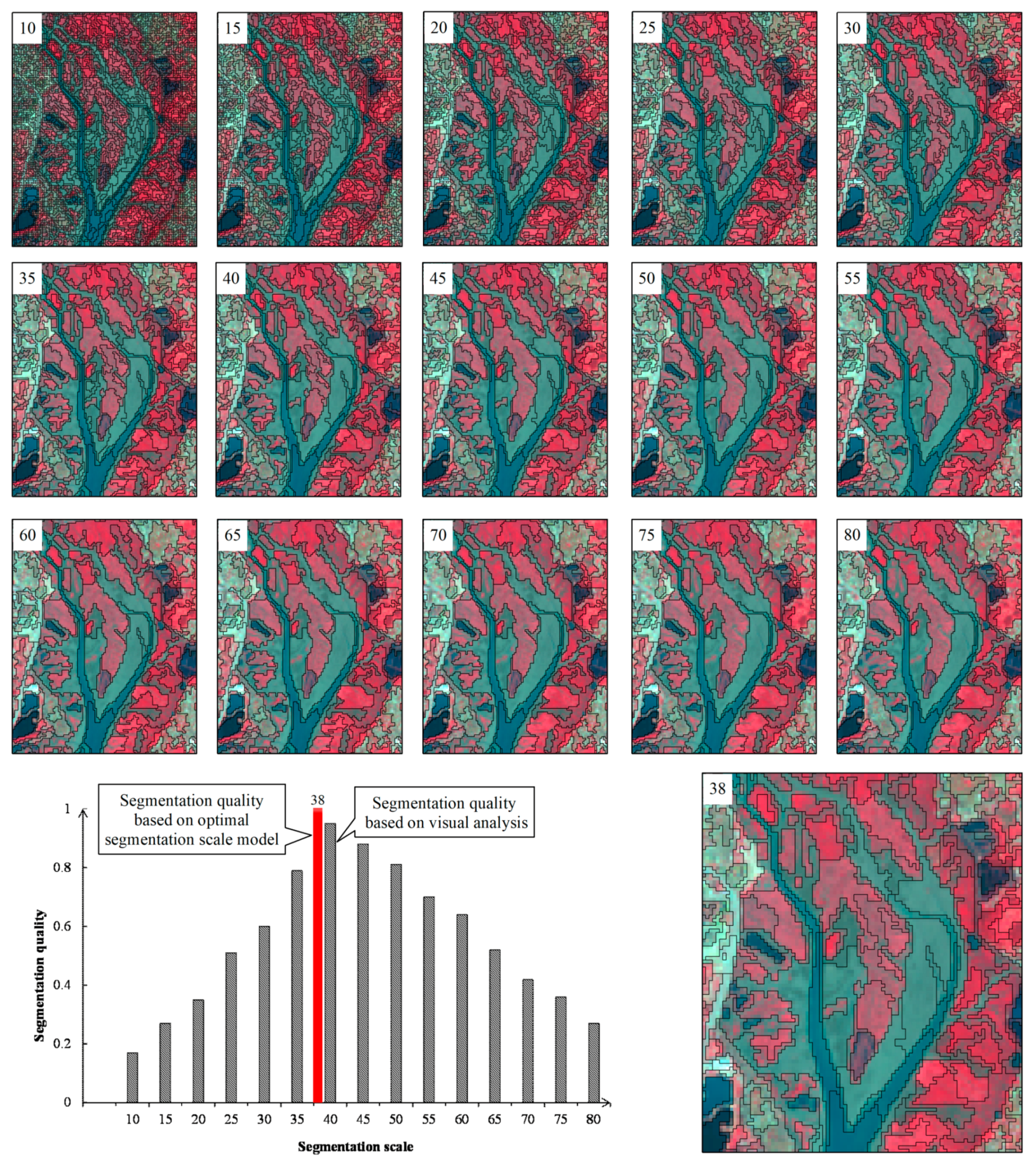
2.4. Optimal Segmentation Scale Model Based on Object-Oriented Classification

To improve the boundary consistency between the segmented image objects and real land cover types, an optimal segmentation scale was applied to process the scale segmentation and selection. It is assumed that when the internal homogeneity (i.e., no mixed objects) and neighboring heterogeneity (i.e., high differentiation among adjacent objects) of segmented objects reaches their optimum, the segmentation scale is optimal. The basic concept of the optimal segmentation scale model was referenced by Chabrier et al. [38] and Espindola et al. [39]. Using the model, the relationship between the internal homogeneity and the heterogeneity of segmented objects is expressed by the segmentation quality function, which can objectively evaluate the quality of segmentation effects. In order to obtain the optimal segmentation scale, a series of pre-segmentation experiments for different segmentation scale was performed. In the study, a segmented image series was obtained using 15 different scales, which started with a scale parameter of 10 and ended at 80, increasing by increments of 5.

Apart from the segmentation scale, the image segmentation parameters also included shape and compactness factor, which were determined by referencing previous studies and from practical experience [31]. After segmentation, the image objects were classified into specific land cover types using a decision tree and visual interpretation.

2.5. Mangrove Forest Change

To analyze and assess the dynamic degree of mangrove forests objectively, the annual land change rate (ALCR) of each land cover type was calculated, which is expressed as follows [40]:

$$ALCR=\frac{U_b-U_a}{U_a}\times \frac{1}{T}\times 100\%$$

(1)

where U_a and U_b represent the area of each land cover type at the beginning and the end of the study period, respectively. T is the number of years. In the study, the time interval was divided into 4 stages: 1990–1997, 1997–2005, 2005–2010 and 2010–2017.

The invasive species of Spartina (Spartina anglica and Spartina alterniflora) pose a significant threat to the existence and expansion of mangrove forests [41]. From the perspective of species competition, the adverse effects of Spartina on mangrove forests can be reflected by analyzing the spatial and temporal reproduction intensity of Spartina. An exponential growth model was applied to describe the expansion of Spartina, which is calculated as follows [31]:

$$S_b=S_a\times {(1+p)}^n$$

(2)

where S_a and S_b are defined as the area of Spartina in the beginning year and ending year in each stage, respectively; n is the number of years; and p is the annual expansion rate of Spartina.

In addition, to analyze the characteristics of spatial change of mangrove forests more explicitly, an overlay analysis in ArcGIS 10 [42] was used to create a conversion matrix between mangrove forests and other land cover types for the time periods 1990–1997, 1997–2005, 2005–2010 and 2010–2017. Meanwhile, a Sankey diagram [43] was used to illustrate the conversion results of each land cover type, which can visualize the dynamics of total land cover types.

2.6. Calculation of Centroid Migration

Centroid migration of different landscapes can reflect their development characteristics in terms of spatial and temporal scales [44]. Analysis of the centroid change of mangrove forests and other land cover types not only allows for the quantitative investigation of the spatial and temporal evolution (direction and distance) of mangrove forests, but also the relationship between mangrove forests and other land cover types. For this purpose, the centroid migrations of mangrove forests and Spartina were analyzed. The equation of centroid is expressed as follows [45]:

$$X_t=\frac{{\displaystyle \sum _{i=1}^n(C_{ti}{X}_i)}}{{\displaystyle \sum _{i=1}^n{C}_{ti}}},Y_t=\frac{{\displaystyle \sum _{i=1}^n(C_{ti}{Y}_i)}}{{\displaystyle \sum _{i=1}^n{C}_{ti}}}$$

(3)

where X_t and Y_t represent the latitude and longitude coordinates of the centroid for one land cover type in the t year, respectively, X_i and Y_i are the latitude and longitude coordinates for the centroid of the ith patch for one land cover type, C_ti is the area of the ith patch, and n is the number of patches for one land cover type.

3. Results

3.1. Optimal Segmentation Scale

We determined the optimal segmentation scale using the optimal segmentation scale model. The segmentation effect and the segmentation quality of different segmentation scales are shown in Figure 3. According to Figure 3, when the segmentation scale was less than 30, the image was over-segmented and one real geo-object was fragmented by more than one resulting segment. When the segmentation scale was greater than 60, the image was under-segmented and one resulting segment covered an area that did not belong to the target geo-object. Moreover, as the segmentation scale increased, additional time was required to segment. Using qualitative visual analysis, we found that the best segmentation effect occurred when the segmentation scale equaled 40, and the corresponding segmentation quality was 0.95. The optimal segmentation scale model calculated the optimal segmentation scale to be 38 and the corresponding segmentation quality was 0.99. The segmentation quality of the optimal segmentation scale obtained by optimal segmentation scale model was better than that of visual judgment.

3.2. Temporal and Spatial Changes of Mangrove Forests

Combining the object-oriented classification, decision tree and visual interpretation, we produced land cover maps of the study area (Figure 4).

Table 3. Summary of land cover classification accuracies from 1990 to 2017.

Land Cover Type	1990		1997		2005		2010		2017
	Pro	Use	Pro	Use	Pro	Use	Pro	Use	Pro	Use
Mangrove	0.96	0.92	0.96	0.92	0.96	0.92	0.96	0.93	0.95	0.97
Spartina	0.90	0.90	0.92	0.92	0.93	0.93	0.93	0.93	0.97	0.91
Mudflat	0.93	0.93	0.91	0.91	0.89	0.89	0.94	0.94	0.94	0.94
Water body	0.94	1.00	0.94	0.94	0.94	0.94	0.89	0.94	0.88	0.93
Aquaculture pond	0.95	1.00	0.90	1.00	0.90	1.00	0.90	0.95	0.92	0.96
Built-up area	0.89	0.80	0.89	0.80	0.89	0.80	0.89	0.89	0.91	0.91
Woodland	0.88	1.00	0.88	1.00	0.86	1.00	0.88	0.88	0.92	0.92
Cropland	1.00	1.00	0.86	1.00	0.86	1.00	0.86	1.00	0.88	1.00
Grassland	0.88	0.88	0.89	0.80	0.89	0.80	0.89	0.80	0.90	0.82
Barren land	0.89	0.80	0.88	0.78	0.89	0.80	1.00	0.88	1.00	0.90
Overall accuracy	0.93		0.91		0.91		0.92		0.93
Kappa coefficient	0.92		0.90		0.90		0.91		0.92

Pro denotes producer accuracy; Use denotes user accuracy.

presents the accuracy assessment results of the land cover types in each study year. The overall accuracies of all the classification results were more than 0.91 and all the Kappa coefficients were more than 0.90, which means that our classification results were consistent with those obtained from the validation points.

Table 4. Change area and annual land change rate (ALCR) of land cover types in study area.

Land Cove Type	1990–997		1997–2005		2005–2010		2010–2017		1990–2017
	Change Area/km2	ALCR/%	Change Area/km2	ALCR/%	Change Area/km2	ALCR/%	Change Area/km2	ALCR/%	Change Area/km2	ALCR/%
Mangrove	0.09	14.29	−0.02	−1.39	0.62	77.5	1.79	32.78	2.48	102.06
Spartina	0.79	38.92	3.15	36.46	2.10	9.93	1.80	4.06	7.84	100.13
Aquaculture pond	0.12	1.11	0.68	5.12	−0.19	−1.62	2.96	19.67	3.57	8.59
Mudflat	−0.83	−0.27	−4.51	−1.33	−3.63	−1.92	−6.78	−2.83	−15.75	−1.35
Water body	0.00	0.00	0.14	0.07	−0.20	−0.17	−0.19	−0.12	−0.25	−0.04
Grassland	0.01	7.14	0.02	8.33	0.04	16.00	0.06	9.52	0.13	24.07
Cropland	0.13	9.77	−0.10	−3.91	−0.02	−1.82	0.00	0.00	0.01	0.19
Woodland	0.06	0.61	0.05	0.43	0.03	0.39	0.03	0.28	0.17	0.45
Built-up area	−0.36	−4.15	0.56	7.95	0.57	7.92	0.99	7.04	1.76	5.26
Barren land	0.00	0.00	0.01	12.50	0.67	670	−0.65	−13.46	0.03	11.11

shows the change area and ALCR of each land cover type. The comparison in extent of mangrove, Spartina and aquaculture pond are illustrated in Figure 5. The results indicate that the mangrove forests experienced a general increasing trend from 0.09 km² in 1990 to 2.57 km² in 2017, with a change rate of 0.09 km²/y and an ALCR of 102.06%. The mangrove forest area decreased only in the period 1997‒2005, while from 2010 to 2017, the mangrove forest area increased rapidly. Spartina exhibited a dramatic increase from 1990 to 2017, implying an average rate of gain of 0.29 km²/y. During 1997‒2005, Spartina expanded markedly, in contrast to the mangrove forest change trend during this period. The distribution range of Spartina expanded from sporadic patches on the West Luoyang River in 1990 to large-scale continuous stands along both sides of the Luoyang River in 2017. During the period 1990‒2017, aquaculture ponds more than tripled in area (from 1.54 to 5.14 km²). Built-up areas increased by 1.76 km² from 1990 to 2017. Although there were small changes in area, the ALCR of grassland and barren land were 24.07% and 11.11%, respectively, which were relatively higher than other land cover types from 1990 to 2017. In contrast, mudflats decreased sharply with a loss of 15.75 km² during 1990‒2017.

The Sankey diagram visualizes the dynamics of total land cover types from 1990 to 2017 (Figure 6a). The results show that mudflats were the principal land cover type invaded by Spartina. The area of Spartina expansion in mudflats was 65.98, 334.08, 305.45 and 412.37 ha during 1990–1997, 1997–2005, 2005–2010, and 2010–2017, respectively, which suggests an increase over time. However, the annual expansion rate for Spartina was 20.66%, 18.61%, 8.40% and 3.64% during 1990–1997, 1997–2005, 2005–2010, and 2010–2017, respectively, suggesting a progressive decline.

3.3. Conversions between Mangrove Forests and Other Land Cover Types

Figure 6b and

Table 5. Conversion comparison between mangrove forests and other land cover types in the Quanzhou Bay Estuary Wetland Nature Reserve (QBEWNR).

Change Type	Conversion Area/ha
	1990–1997	1997–2005	2005–2010	2010–2017
Mangrove → Cropland	—	1.12	—	—
Mangrove → Spartina	—	2.21	—	0.54
Mangrove → Built-up area	0.13	1.36	0.87	0.74
Mangrove →Aquaculture pond	—	0.25	—	—
Mangrove → Mudflat	1.37	2.49	3.00	0.90
Spartina → Mangrove	—	—	7.20	46.22
Built-up area → Mangrove	4.81	—	0.09	0.06
Aquaculture pond → Mangrove	0.69	0.02	0.38	2.75
Mudflat → Mangrove	5.22	5.22	57.81	132.38

illustrate the spatial distribution and area of conversion between mangrove forests and other land cover types. It was found that the conversion region gradually expanded, and the most marked mangrove forest recession occurred from 1997 to 2005, attributed to a large area conversion to mudflats and Spartina, which accounted for 33.51% and 29.74% of mangrove forest reduction in this stage, respectively. During the period 2010‒2017, nearly 181 ha of other land cover types were transformed into mangrove forests and resulted in a significant expansion of mangrove forests in this stage. The proportion of mudflats and Spartina converted into mangrove forests were the highest of the different land cover types, accounting for 72.97% and 25.48%, respectively. There was little conversion among mangrove forests and cropland, built-up areas or aquaculture ponds during the study period. These results suggest that the change in mangrove forest area can be attributed to their expansion in mudflats and the ecological competition with Spartina.

The centroid migration routes of mangrove forests and Spartina are displayed in Figure 7. From 1990 to 2017, the centroid of mangrove forests experienced a trend of shifting landward before 1997 and a process of shifting seaward after 1997. The centroid of Spartina showed a persistent seaward migration throughout the study period. It is noteworthy that the distance between the mangrove forest centroid and the centroid of Spartina was increasing, changing from 159.57 m in 1990 to 7308.92 m in 2017.

4. Discussion

4.1. Mangrove Forest Losses Associated by Human Activities and Possible Environmental Threats

Spartina, as invasive plant species, were first introduced to China’s coastal provinces from the Atlantic Coast of the U.S. for coastal environment promotion in 1976 [46]. However, due to their rapid growth, high productivity and strong adaptability, introduced Spartina expanded rapidly in tidal zones and now pose a tremendous threat to native biodiversity. Once Spartina have invaded the mangrove forest gaps, they inhibit the germination and growth of mangrove seedlings by competing for space, light and nutrients [47,48]. Our results found that the propagation of mangrove forests was suppressed where they grew in or around Spartina (Figure 4). Conversion to Spartina was the primary contributor of mangrove forest losses, especially from 1997 to 2005 (Table 5). Previous studies have also shown Spartina expansion increased the pressure on survival and breeding of mangrove forests [48,49], which is consistent with our findings. Moreover, in other coastal zones of China, for instance, Shankou of Guangxi province, Qi’ao island, and Shenzhen Bay, Spartina invasion has become one of the most serious threats to mangrove forest growth [41,45,50]. Spartina can become established in mudflats, easily resulting in the loss of suitable habitats which are available for mangrove forest reproduction [31,51]. Our results also showed that the Spartina area increased by 7.84 km² with an ALCR of 100.13% from 1990 to 2017, with mudflats as the priority areas of encroachment (Table 4, Figure 4, Figure 5 and Figure 6). Without effective systematic intervention, we posit that Spartina would gradually cover the entire intertidal mudflat and become an irrevocable threat to mangrove ecosystems. Figure 8a,b illustrates the inhibition of mangrove seedling growth by Spartina and its expansion in mudflats, respectively.

Aquaculture development is another factor that has contributed to the losses of mangrove forest in the QBEWNR. Over the period 1990–2017, aquaculture ponds increased significantly by 3.57 km² (Figure 5) and most were established in mudflat areas (Figure 4 and Figure 6). Diseases caused by aquaculture have a negative effect on mangrove forests [52]. The untreated water discharged by aquaculture can bring more pressures against the nutrient load in water bodies. Once the self-purification capacity of water bodies has been exceeded, the health of mangrove forests faces serious threats [53]. In addition, suitable habitat for mangrove forests was encroached upon by constructing aquaculture ponds in mudflats. Consequently, the losses of mangrove forests were due to aquaculture expansion to some extent. In previous studies, researchers have indicated that of the one-third of mangrove forests that have disappeared worldwide in the last 30 years, 35% was lost to aquaculture; this figure may reach 60% by 2030 [54,55]. Figure 8c,d displays aquaculture ponds located adjacent to mangrove forests and aquaculture development in mudflats, respectively.

Due to their location in low coastal elevation areas, mangrove forests are particularly vulnerable to sea-level rise [56,57,58]. Previous research on sea-level change has reported that the sea-level of the Fujian coastal zone increased at an average rate of 2 mm/y during the last half century [59]. In response to rising sea-levels, mangrove forests are more likely to migrate landward [30,60]. However, such a landward migration and establishment has been obstructed by artificial seawalls in the study area (Figure 9), which meant that mangrove forests could only expand seaward. In addition, the roots of mangrove forests should be exposed to the air at a certain time, otherwise they would not be able to complete their own physiological processes and propagation [58,61,62]. As a result of sea-level rise, lower elevation areas would be inundated and waterlogged longer, which means mangrove forests would not meet the time required for mangrove root respiration, so mangrove forests cannot easily establish and propagate seaward.

As shown in Figure 10, the annual average temperature and annual precipitation both increased in the QBEWNR from 1990 to 2017. Although a warmer and wetter climate would favor the establishment of mangrove forests [63], such climate change would promote sea-level rise, leading directly to the space loss of mangrove forest expansion seaward. Therefore, it is evident that, in the context of global warming, the potential for major coastal change aggravates the survival risk and pressures of seaward succession for mangrove forests. Overall, as for the study area, climate change and sea-level rise would potentially have adverse effects on mangrove forests.

4.2. Positive Effects of Reforestation Projects and Spartina Control

One notable caveat to these results is that the area of mangrove forests in the QBEWNR was only 0.09 km² in 1990, had doubled to 0.18 km² in 1997, and then declined to 0.16 km² in 2005. These areas represent a limited distribution. Since 2005, mangrove forests have increased rapidly (Figure 5 and Figure 6). Under the ecological restoration schemes for coastal wetlands in Quanzhou Bay, various national and local ecological conservation projects have been carried out since 2000, including “National Wetland Conservation and Restoration”, “Marine Environment Ecological Restoration Project in Quanzhou Bay”, and “Mangrove Forest Restoration Project in Luoyang River” [64]. One of the common objectives for these ecological engineering projects is to cultivate and replant mangrove forests (i.e., reforestation projects) to increase mangrove forest area. According to the previous report [65], the afforestation area of mangrove forests was approximately 200 ha until 2015, indicating an 80%‒85% increase in mangrove forests because of the reforestation projects. Studies focusing on the mangrove forest dynamics in China from 1973 to 2015 had indicated that protection and reforestation actions had supported mangrove forest restoration greatly, which is consistent with our results [30]. Figure 8e,f demonstrates a monument of mangrove forest reforestation project and the mangrove seedling cultivation base, respectively.

Although awareness of the need to protect mangrove forests has increased, the threats of Spartina invasion and the importance of Spartina control were recognized relatively late in China [30,66]. This probably explains why reforestation engineering was implemented in 2000, but the mangrove forests continued to decrease between 1997 and 2005 (Table 4). Since 2007, both national and local agencies have promoted the implementation and enforcement of Spartina control projects in the QBEWNR [67]. Up to 2017, the area of Spartina converted to mangrove forests had increased to 53.42 ha, including 7.20 ha from 2005 to 2010 and 46.22 ha from 2010 to 2017 (Table 5). Meanwhile, the annual expansion rate of Spartina had declined from 20.66% at the beginning of the same period, to 3.64% at the end. Moreover, the centroid distance between Spartina and mangrove forests has increased (Figure 7). Therefore, it can be inferred that, due to the management and control of Spartina, the disturbance caused by Spartina to mangrove forests has been mitigated to some degree. Figure 8g,h show the specific implementation scenario and subsequent effects of Spartina control, respectively.

As mentioned above, whether through mangrove forest reforestation projects or Spartina control, the performance of conservation activities plays a substantial role in the existence and expansion of mangrove forests, which to a large extent neutralizes or offsets the losses of mangrove forests caused by negative factors.

4.3. Suggestions for Conserving and Managing Mangrove Forests

Monitoring and dynamic change analysis for mangrove forests are critical for their conservation and management, and to help with formulating and implementing government policies [68,69]. The results from this study on the spatio-temporal change of mangrove forests and conversion between mangrove forests and other land cover types (Figure 4, Figure 5 and Figure 6, Table 4 and Table 5) can be used as a guideline for conserving and managing mangrove forests.

First, the implementation of artificial afforestation projects should be continued to increase the area of mangrove forests. Establishing a mangrove forest monitoring system is also indispensable and would allow for the elimination and control of insect pests and effective feedback on all aspects of mangrove forests. Meanwhile, cutting mangrove forests indiscriminately and disposing of rubbish within mangrove forests must be prohibited. Second, prevention and control of Spartina should be further studied, and more feasible measures should be taken to impede the expansion of Spartina in mudflats, with the aim of restoring suitable habitat for mangrove forests. For the zones in which Spartina has been eradicated, breeding conditions should be monitored regularly. Third, strict limitations on aquaculture development should be implemented in the reserve, and the pollution problems caused by aquaculture must be contained. Fourth, in focusing on the important ecological value of mangrove forests, local managers and conservationists should reinforce mangrove forest conservation by teaching local residents about the conservation implications and by disseminating information about the severe threats faced by mangrove forests.

4.4. Advantages and Uncertainties of the Methods for Mangrove Forest Monitoring

So far, the primary segmentation scale determination approach is based on visual analysis, which is subjective and cannot effectively avoid over-segmentation and under-segmentation errors [70]. The optimal segmentation scale model used in our study not only gave a quantitative result, which is based on objective evaluation, but also kept better boundary consistency between the segmented image objects and real land cover types (Figure 3). Moreover, in the visual interpretation process, the manual modification of objects obtained using the optimal segmentation scale model was less than the objects generated through visual analysis determining the best scale, which improved classification efficiency and reduced the workload of interpreters.

Classification accuracy can be improved by using the spectral difference among different land cover types effectively [71]. In this study, the spectral discrimination of mangrove forests, Spartina, and mudflats derived from seasonal change was given a full comparison and analysis, and we found that they were more accurately distinguished than in previous research [21,30,31]. Therefore, multi-seasonal images appear to be feasible and desirable data sources for monitoring mangrove forests located in subtropical areas. In tropical zones, owing to very small phenological differences, it may be difficult to discern spectral distinction between mangrove forests and Spartina. Accordingly, multi-seasonal images may not be applicable for mapping mangrove forests growing in tropical regions.

Our analysis focused on mangrove forest dynamics over a long time series (from 1990 to 2017). This is significant for maintaining the spatial coherence of classification maps derived from various sensor images. Due to the spatial uncertainties that arose from the scanning system, wavelength setting, over-pass time, and angular effect, unbiased maps were difficult to produce. In addition, several uncertainties and limitations also existed in the segmentation parameter selection. Besides the segmentation scale, the shape and compactness variables, which respectively balance spectral homogeneity with the shape of the objects and the compactness with smoothness, are essential for controlling the clustering decision process of image objects. Although the optimal segmentation scale was determined objectively, the selection of other segmentation factors chosen by referencing previous research was subjective.

5. Conclusions

Considering the importance of tidal information for mangrove forest monitoring and the spectral differences among mangrove forests, mudflats, and Spartina, several multi-seasonal Landsat images acquired during low tide were selected as the basic data sources. Combining an optimal segmentation scale model based on object-oriented classification, centroid migration calculations and spatial analysis, we discerned dynamic changes in the mangrove forest and their influencing factors in the QBEWNR from 1990 to 2017. Our results showed that there were some advantages for the approaches used in this study for mangrove forest monitoring, since the classification accuracy and efficiency of land cover map improved. Mangrove forests significantly expanded during the period of 1990–2017: the total area increased by 2.48 km², with a dynamic degree of 102.06%. Most of the expanding mangrove forests transitioned from mudflats and Spartina. Mangrove forest changes were influenced by many factors. Environmental threats, including climate change and sea-level rise, Spartina invasion and aquaculture development exerted negative effects, while reforestation projects and Spartina control had a positive effect. In this study, the role of the latter was greater than the former. We demonstrated that conservation activities benefit the existence and expansion of mangrove forests. These conclusions can be used as a guide for governments and conservationists to make policies and effectively protect and monitor mangrove forests.

References

1. Costanza, R.; Groot, R.D.; Sutton, P.; Ploeg, S.V.D.; Anderson, S.J.; Kubiszewski, I.; Farber, S.; Turner, R.K. Changes in the global value of ecosystem services. Glob. Environ. Chang. 2014, 26, 152–158. [Google Scholar] [CrossRef]
2. Brown, M.I.; Pearce, T.; Leon, J.; Sidle, R.; Wilson, R. Using remote sensing and traditional ecological knowledge (TEK) to understand mangrove change on the Maroochy River, Queensland, Australia. Appl. Geogr. 2018, 94, 71–83. [Google Scholar] [CrossRef]
3. Pham, T.D.; Kaida, N.; Yoshino, K.; Xuan, H.N.; Bui, D.T. Willingness to pay for mangrove restoration in the context of climate change in the Cat Ba biosphere reserve, Vietnam. Ocean Coast. Manag. 2018, 163, 269–277. [Google Scholar] [CrossRef]
4. Kathiresan, K.; Bingham, B.L. Biology of mangroves and mangrove Ecosystems. Adv. Mar. Biol. 2001, 40, 81–251. [Google Scholar]
5. Giri, C.; Ochieng, E.; Tieszen, L.L.; Zhu, Z.; Singh, A.; Loveland, T.; Masek, J.; Duke, N. Status and distribution of mangrove forests of the world using earth observation satellite data. Glob. Ecol. Biogeogr. 2011, 20, 154–159. [Google Scholar] [CrossRef]
6. Jia, M.M.; Liu, M.Y.; Wang, Z.M.; Mao, D.H.; Ren, C.Y.; Cui, H.S. Evaluating the effectiveness of conservation on mangroves: A remote sensing-based comparison for two adjacent protected areas in Shenzhen and Hong Kong, China. Remote Sens. 2016, 8, 627. [Google Scholar] [CrossRef]
7. Gao, Y.; Yu, G.R.; Yang, T.T.; Jia, Y.L.; He, N.P.; Zhuang, J. New insight into global blue carbon estimation under human activity in land-sea interaction area: A case study of China. Earth-Sci. Rev. 2016, 159, 36–46. [Google Scholar] [CrossRef] [Green Version]
8. Pham, T.D.; Yoshino, K.; Le, N.; Bui, D.T. Estimating aboveground biomass of a mangrove plantation on the northern coast of Vietnam using machine learning techniques with an integration of ALOS-2 PALSAR-2 and Sentinel-2A data. Int. J. Remote Sens. 2018. [Google Scholar] [CrossRef]
9. Pham, T.D.; Yoshino, K.; Bui, D.T. Biomass estimation of Sonneratia caseolaris (L.) Engler at a coastal area of Hai Phong city (Vietnam) using ALOS-2 PALSAR imagery and GIS-based multi-layer perceptron neural networks. GISci. Remote Sens. 2017, 54, 329–353. [Google Scholar] [CrossRef]
10. Tamooh, F.; Huxham, M.; Karachi, M.; Mencuccini, M.; Kairo, J.G.; Kirui, B. Below-ground root yield and distribution in natural and replanted mangrove forests at Gazi bay, Kenya. For. Ecol. Manag. 2008, 256, 1290–1297. [Google Scholar] [CrossRef]
11. Alongi, D.M. Carbon sequestration in mangrove forests. Carbon Manag. 2012, 3, 313–322. [Google Scholar] [CrossRef]
12. Kauffman, J.B.; Heider, C.; Norfolk, J.; Payton, F. Carbon stocks of intact mangroves and carbon emissions arising from their conversion in the Dominican Republic. Ecol. Appl. 2013, 24, 518–527. [Google Scholar] [CrossRef]
13. Cavanaugh, K.C.; Kellner, J.R.; Forde, A.J.; Gruner, D.S.; Parker, J.D.; Rodriguez, W.; Feller, I.C. Poleward expansion of mangroves is a threshold response to decreased frequency of extreme cold events. Proc. Natl. Acad. Sci. USA 2014, 111, 723–727. [Google Scholar] [CrossRef] [PubMed]
14. Chen, B.Q.; Xiao, X.M.; Li, X.P.; Pan, L.H.; Doughty, R.; Ma, J.; Dong, J.W.; Qin, Y.W.; Zhao, B.; Wu, Z.X.; et al. A mangrove forest map of China in 2015: Analysis of time series Landsat 7/8 and Sentinel-1A imagery in Google Earth Engine cloud computing platform. ISPRS J. Photogramm. Remote Sens. 2017, 131, 104–120. [Google Scholar] [CrossRef]
15. Rahman, A.F.; Dragoni, D.; Didan, K.; Barreto-Munoz, A.; Hutabarat, J.A. Detecting large scale conversion of mangroves to aquaculture with change point and mixed-pixel analyses of high-fidelity MODIS data. Remote Sens. Environ. 2014, 130, 96–107. [Google Scholar] [CrossRef]
16. Giri, C.; Long, J.; Abbas, S.; Murali, R.M.; Qamer, F.M.; Pengra, B.; Thau, D. Distribution and dynamics of mangrove forests of South Asia. J. Environ. Manag. 2015, 148, 101–111. [Google Scholar] [CrossRef] [PubMed]
17. Matthews, G.V.T. The Ramsar Covention on Wetlands: Its History and Development; Secretariat, R.C., Ed.; Imprimerie Dupuis SA: Gland, Switzerland, 2013. [Google Scholar]
18. Hu, L.J.; Li, W.Y.; Xu, B. Monitoring mangrove forest change in China from 1990 to 2015 using Landsat-derived spectral-temporal variability metrics. Int. J. Appl. Earth Obs. Geoinf. 2018, 73, 88–98. [Google Scholar] [CrossRef]
19. Kuenzer, C.; Bluemel, A.; Gebhard, S.; Vo Quoc, T.; Dech, S. Remote sensing of mangrove ecosystems: A review. Remote Sens. 2011, 3, 878–928. [Google Scholar] [CrossRef]
20. Heumann, B.W. Satellite remote sensing of mangrove forests: Recent advances and future opportunities. Prog. Phys. Geogr. 2011, 35, 87–108. [Google Scholar] [CrossRef]
21. Jia, M.; Wang, Z.; Li, L.; Song, K.; Ren, C.; Liu, B.; Mao, D. Mapping China’s mangroves based on an object-oriented classification of Landsat imagery. Wetlands 2014, 34, 277–283. [Google Scholar] [CrossRef]
22. Tian, J.Y.; Wang, L.; Li, X.J.; Gong, H.L.; Shi, C.; Zhong, R.F.; Liu, X.M. Comparison of UAV and WorldView-2 imagery for mapping leaf area index of mangrove forest. Int. J. Appl. Earth Obs. Geoinf. 2017, 61, 22–31. [Google Scholar] [CrossRef]
23. Wang, L.; Silván-Cárdenas, L.; Sousa, W.P. Neural network classification of mangrove species from multi-seasonal IKONOS imagery. Photogramm. Eng. Remote Sens. 2008, 74, 921–927. [Google Scholar] [CrossRef]
24. Lee, T.M.; Yeh, H.C. Applying remote sensing techniques to monitor shifting wetland vegetation: A case study of Danshui River estuary mangrove communities, Taiwan. Ecol. Eng. 2009, 35, 487–496. [Google Scholar] [CrossRef]
25. Ibharim, N.A.; Mustapha, M.A.; Lihan, T.; Mazlan, A.G. Mapping mangrove changes in the Matang Mangrove Forest using multi temporal satellite imageries. Ocean Coast. Manag. 2015, 114, 64–76. [Google Scholar] [CrossRef]
26. Castillo, J.A.A.; Apan, A.A.; Maraseni, T.N.; Salmo, S.G. Estimation and mapping of above-ground biomass of mangrove forests and their replacement land uses in the Philippines using Sentinel imagery. ISPRS J. Photogramm. 2017, 134, 70–85. [Google Scholar] [CrossRef]
27. Cissell, J.R.; Delgado, A.M.; Sweetman, B.M.; Steinberg, M.K. Monitoring mangrove forest dynamics in Campeche, Mexico, using Landsat satellite data. Remote Sens. Appl. Soc. Environ. 2018, 9, 60–68. [Google Scholar] [CrossRef]
28. Xia, Q.; Qin, C.Z.; Li, H.; Huang, C.; Su, F.Z. Mapping mangrove forests based on multi-tidal high-resolution satellite imagery. Remote Sens. 2018, 10, 1343. [Google Scholar] [CrossRef]
29. Baatz, M.; Schäpe, A. Multiresolution Segmentation: An Optimization Approach for High Quality Multi-Scale Image Segmentation. 2000. Available online: http://www.ecognition.com/sites/default/files/405_baatz_fp_12.pdf (accessed on 25 October 2018).
30. Jia, M.M.; Wang, Z.M.; Zhang, Y.Z.; Mao, D.H.; Wang, C. Monitoring loss and recovery of mangrove forests during 42 years: The achievements of mangrove conservation in China. Int. J. Appl. Earth Obs. Geoinf. 2018, 73, 535–545. [Google Scholar] [CrossRef]
31. Liu, M.Y.; Li, H.Y.; Li, L.; Man, W.D.; Jia, M.M.; Wang, Z.M.; Lu, C.Y. Monitoring the invasion of Spartina alterniflora using multi-source high-resolution imagery in the Zhangjiang Estuary, China. Remote Sens. 2017, 9, 539. [Google Scholar] [CrossRef]
32. Conchedda, G.; Durieux, L.; Mayaux, P. An object-based method for mapping and change analysis in mangrove ecosystems. ISPS J. Photogramm. 2008, 63, 578–589. [Google Scholar] [CrossRef]
33. Su, T.F.; Zhang, S.W. Local and global evaluation for remote sensing image segmentation. ISPS J. Photogramm. 2017, 130, 256–276. [Google Scholar] [CrossRef]
34. Schultz, B.; Immitzer, M.; Formaggio, A.R.; Sanches, I.D.A.; Luiz, A.J.B.; Atzberger, C. Self-Guided segmentation and classification of multi-temporal Landsat 8 images for crop type mapping in Southeastern Brazil. Remote Sens. 2015, 7, 14482–14508. [Google Scholar] [CrossRef]
35. D’Antonio, C.M.; Hobbie, S.E. Plant species effects on ecosystem processes: Insights from invasive species. In Species Invasions: Insights into Ecology, Evolution and Biogeography; Sax, D.F., Stachowicz, J.J., Gaines, S.D., Eds.; Sinauer Associates, Inc.: Sunderland, UK, 2005; pp. 65–84. [Google Scholar]
36. FLAASH User’s Guide; ENVI FLAASH Version 4.1; Research Systems, Inc.: Boulder, CO, USA, 2004; pp. 1–80.
37. Congalton, R.; Green, K. Assessing the Accuracy of Remotely Sensed Data: Principles and Practices; Mapping Science Series; CRC Press: Boca Raton, FL, USA, 2009. [Google Scholar]
38. Chabrier, S.; Emile, B.; Rosenberger, C.; Laurent, H. Unsupervised performance evaluation of image segmentation. EURASIP J. Adv. Signal Process. 2006, 1, 1–12. [Google Scholar] [CrossRef]
39. Espindola, G.M.; Camara, G.; Reis, I.A.; Bins, L.S.; Monteiro, A.M. Parameter selection for region-growing image segmentation algorithms using spatial autocorrelation. Int. J. Remote Sens. 2006, 27, 3035–3040. [Google Scholar] [CrossRef]
40. Zhang, J.Y.; Ma, K.M.; Fu, B.J. Wetland loss under the impact of agricultural development in the Sanjiang Plain, NE China. Environ. Monit. Assess. 2010, 166, 139–148. [Google Scholar] [CrossRef] [PubMed]
41. Wan, H.; Wang, Q.; Jiang, D.; Fu, J.; Yang, Y.; Liu, X. Monitoring the invasion of Spartina alterniflora using very high resolution unmanned aerial vehicle imagery in Beihai, Guangxi (China). Sci. World J. 2014, 2014, 638296. [Google Scholar] [CrossRef] [PubMed]
42. ESRI Inc. ArcGIS Desktop: Release 10, Environmental Systems Research Institute: Redlands, CA, USA, 2011.
43. Cuba, N. Research note: Sankey diagrams for visualizing land cover dynamics. Landsc. Urban Plan. 2015, 139, 163–167. [Google Scholar] [CrossRef]
44. Li, H.Y.; Man, W.D.; Li, X.Y.; Ren, C.Y.; Wang, Z.M.; Li, L.; Jia, M.M.; Mao, D.H. Remote sensing investigation of anthropogenic land cover expansion in the low-elevation coastal zone of Liaoning Province, China. Ocean Coast. Manag. 2017, 148, 245–259. [Google Scholar] [CrossRef]
45. Jia, M.M.; Wang, Z.M.; Zhang, Y.Z.; Ren, C.Y.; Song, K.S. Landsat-based estimation of mangrove forest loss and restoration in Guangxi Province, China, influenced by human and natural factors. IEEE J.-STARS 2015, 8, 311–323. [Google Scholar] [CrossRef]
46. Chung, C.H. Forty years of ecological engineering with Spartina plantations in China. Ecol. Eng. 2006, 27, 49–57. [Google Scholar] [CrossRef]
47. Rogers, K.; Saintilan, N.; Heijnis, H. Mangrove encroachment of salt marsh in Western Port Bay, Victoria: The role of sedimentation, subsidence, and sea level rise. Estuar. Coast. 2005, 28, 551–559. [Google Scholar] [CrossRef]
48. Li, Z.J.; Wang, W.Q.; Zhang, Y.H. Recruitment and herbivory affect spread of invasive Spartina alterniflorain China. Ecology 2014, 95, 1972–1980. [Google Scholar] [CrossRef] [PubMed]
49. Zhang, Y.H.; Huang, G.M.; Wang, W.Q.; Chen, L.Z.; Lin, G.H. Interactions between mangroves and exotic Spartina in an anthropogenically disturbed estuary in southern China. Ecology 2012, 93, 588–597. [Google Scholar] [CrossRef] [PubMed]
50. Biswasa, S.R.; Biswasb, P.L.; Limon, S.H.; Yan, E.R.; Xu, M.S.; Khan, M.S.I. Plant invasion in mangrove forests worldwide. For. Ecol. Manag. 2018, 429, 480–492. [Google Scholar] [CrossRef]
51. Zhou, T.; Liu, S.C.; Feng, Z.L.; Liu, G.; Gan, Q.; Peng, S.L. Use of exotic plants to control Spartina alterniflora invasion and promote mangrove restoration. Sci. Rep. 2015, 5, 12980. [Google Scholar] [CrossRef] [PubMed]
52. Jayanthi, M.; Thirumurthy, S.; Muralidhar, M.; Ravichandran, P. Impact of shrimp aquaculture development on important ecosystems in India. Glob. Environ. Chang. 2018, 52, 10–21. [Google Scholar] [CrossRef]
53. Senarath, U.; Visvanathan, C. Environmental issues in brackishwater shrimp aquaculture in Sri Lanka. Environ. Manag. 2001, 27, 335–348. [Google Scholar] [CrossRef] [PubMed]
54. Alongi, D.M. Present state and future of the world’s mangrove forests. Environ. Conserv. 2002, 29, 331–349. [Google Scholar] [CrossRef]
55. Simard, M.; Rivera-Monroy, V.H.; Mancera-Pineda, J.E.; Castañeda-Moya, E.; Twilley, R.R. A systematic method for 3D mapping of mangrove forests based on Shuttle Radar Topography Mission elevation data, ICEsat/GLAS waveforms, and field data: Application to Ciénaga Grande de Santa Marta, Colombia. Remote Sens. Environ. 2008, 112, 2131–2144. [Google Scholar] [CrossRef]
56. Woodruff, J.D. Future of tidal wetlands depends on coastal management. Nature 2018, 561, 183–185. [Google Scholar] [CrossRef] [PubMed]
57. Rodríguez, J.F.; Saco, P.M.; Sandi, S.; Saintilan, N.; Riccardi, G. Potential increase in coastal wetland vulnerability to sea-level rise suggested by considering hydrodynamic attenuation effects. Nat. Commun. 2017, 8, 16094. [Google Scholar] [CrossRef] [PubMed] [Green Version]
58. Lu, W.Z.; Chen, L.Z.; Wang, W.Q.; Tam, N.F.; Lin, G.H. Effects of sea level rise on mangrove Avicennia population growth, colonization and establishment: Evidence from a field survey and greenhouse manipulation experiment. Acta Oecol. 2013, 49, 83–91. [Google Scholar] [CrossRef]
59. Yuan, F.C.; Zhang, W.Z.; Yang, J.X.; Chen, D.W. Study on sea level variability in off shore Fujian. J. Appl. Oceanogr. 2016, 35, 20–32. [Google Scholar]
60. Soares, M.L.G. A conceptual model for the responses of mangrove forests to sea level rise. J. Coast. Res. 2009, 25, 267–271. [Google Scholar]
61. Wang, W.Q.; Wang, M. The Mangrove of China; Science Press: Beijing, China, 2007. [Google Scholar]
62. Rivera-Monroy, V.H.; Twilley, R.R.; Davis, S.E.; Childers, D.L.; Simard, M.; Chambers, R.; Jaffe, R.; Boyer, J.N.; Rudnick, D.T.; Zhang, K.; et al. The role of the everglades mangrove ecotone region (EMER) in regulating nutrient cycling and wetland productivity in South Florida. Crit. Rev. Environ. Sci. Technol. 2011, 41, 633–669. [Google Scholar] [CrossRef]
63. Osland, M.J.; Feher, L.C.; Lopez-Portillo, J.; Day, R.H.; Suman, D.O.; Menéndez, J.M.G.; Rivera-Monroy, V.H. Mangrove forests in a rapidly changing world: Global change impacts and conservation opportunities along the Gulf of Mexico coast. Estuar. Coast. Shelf Sci. 2018, 214, 120–140. [Google Scholar] [CrossRef]
64. Ecological Restoration of Mangrove Forests in Quanzhou Bay. Available online: http://qz.fjsen.com/2013-09/28/content_12612308.htm (accessed on 28 September 2013).
65. National Ecological City “Flowers Bloom All over the City”. Available online: http://www.qzepb.gov.cn/xxgk/ztzl/cjgjsts/gzdt/201609/t20160907_54283.htm (accessed on 7 September 2016).
66. Tan, F.L. Spartina control strategy of China. Wetlands Sci. 2007, 5, 105–110. [Google Scholar]
67. Cai, N.N. Status and strategy of wetland conservation in Quanzhou Bay Estuary. Mod. Agric. Sci. Technol. 2009, 21, 253–254. [Google Scholar]
68. Giri, C.; Zhu, Z.; Tieszen, L.L.; Singh, A.; Gillette, S.; Kelmelis, J.A. Mangrove forest distributions and dynamics (1975–2005) of the tsunami-affected region of Asia. J. Biogeogr. 2008, 35, 519–528. [Google Scholar] [CrossRef] [Green Version]
69. Liu, K.; Li, X.; Shi, X.; Wang, S.G. Monitoring mangrove forest changes using remote sensing and GIS data with decision-tree learning. Wetlands 2008, 28, 336–346. [Google Scholar] [CrossRef]
70. Drǎguţ, L.; Tiede, D.; Levick, S.R. ESP: A tool to estimate scale parameter for multiresolution image segmentation of remotely sensed data. Int. J. Geogr. Inf. Sci. 2010, 24, 859–871. [Google Scholar] [CrossRef]
71. Hesketh, M.; Sánchez-Azofeifa, G.A. The effect of seasonal spectral variation on species classification in the Panamanian tropical forest. Remote Sens. Environ. 2012, 118, 73–82. [Google Scholar] [CrossRef] [Green Version]
Figure 1. Location of the study area (QBEWNR represents the Quanzhou Bay Estuary Wetland Nature Reserve).
Remotesensing 10 02020 g001
Figure 2. Comparisons of image characteristics and spectral reflectance for mangrove forests, Spartina, and mudflats in different seasons. (a) Image of leaf-on season; (b) image of leaf-off season; (c) spectral reflectance curve of leaf-on season for mangrove forests, Spartina, and mudflats; (d) spectral reflectance curve of leaf-off season for mangrove forests, Spartina, and mudflats (A: mangrove forests, B: Spartina, C: mudflats; Band combination Landsat OLI: R: G: B = Band 5: Band 4: Band 3).
Remotesensing 10 02020 g002
Figure 3. Segmentation effects and segmentation quality evaluation with different scales.
Remotesensing 10 02020 g003
Figure 4. Land cover maps of Quanzhou Bay Estuary Wetland Nature Reserve (QBEWNR) from 1990 to 2017.
Remotesensing 10 02020 g004
Figure 5. Change in total area of Mangrove, aquaculture pond and Spartina from 1990 to 2017.
Remotesensing 10 02020 g005
Figure 6. Comparisons of land cover dynamics. (a) Sankey diagram for comparison of total land cover dynamics from 1990 to 2017; (b) spatial distribution of conversion between mangrove forests and other land cover types in four time intervals from the years 1990, 1997, 2005, 2010, and 2017.
Remotesensing 10 02020 g006
Figure 7. Spatial distribution map of centroid migration for mangrove forests and Spartina from 1990 to 2017.
Remotesensing 10 02020 g007
Figure 8. Positive and negative effects for mangrove forests. (a) Spartina invading the mangrove seedling area; (b) Spartina expansion into mudflats; (c) aquaculture ponds as a threat to mangrove forests; (d) aquaculture development in mudflats; (e) mangrove seedling milestone recorded during the mangrove afforestation project carried out initially in 2001; (f) mangrove seedling cultivation base; (g) artificial control of Spartina by mowing; (h) Spartina were cut off.
Remotesensing 10 02020 g008aRemotesensing 10 02020 g008b
Figure 9. Artificial seawalls with landward mangrove forests. (a) Artificial seawall located in the western boundary of the study area; (b) artificial seawall located in the eastern boundary of the study area.
Remotesensing 10 02020 g009
Figure 10. Change in annual average temperature and annual precipitation in the Quanzhou Bay Estuary Wetland Nature Reserve (QBEWNR) from 1990 to 2017. (a) Annual average temperature in QBEWNR from 1990 to 2017; (b) annual precipitation in QBEWNR from 1990 to 2017.
Remotesensing 10 02020 g010