A Novel Method for High-Voltage Bundle Conductor Reconstruction from Airborne LiDAR Data


1
State Key Laboratory of Information Engineering in Surveying, Mapping and Remote Sensing, Wuhan University, Wuhan 430079, China
2
Collaborative Innovation Center of Geospatial Technology, Wuhan University, Wuhan 430079, China
3
School of Computer Science, China University of Geosciences, Wuhan 430074, China
*
Author to whom correspondence should be addressed.
Remote Sens. 2018, 10(12), 2051; https://doi.org/10.3390/rs10122051
Submission received: 26 October 2018
/
Revised: 4 December 2018
/
Accepted: 15 December 2018
/
Published: 17 December 2018
(This article belongs to the Special Issue Future Trends and Applications for Airborne Laser Scanning)
Abstract
:The security of high-voltage power transmission corridors is significantly vital to the national economy and daily life. With its rapid development, LiDAR (Light Detection and Ranging) technology has been widely applied in the inspection of transmission lines. As the basis of potential hazard detection, a robust and precise power line model is a necessary requirement for rapid and correct clearance. Thus, this paper proposes a novel method for high-voltage bundle conductor reconstruction, which can precisely reconstruct each sub-conductor. First, points in high-voltage power transmission corridors are detected and classified into four categories; second, for classified power lines, single power line spans are extracted, and bundle conductors are identified by analyzing the single spans’ fitting residuals; and then, each sub-conductor of bundle conductors is extracted by a projected dichotomy method on the XOY and XOZ planes, respectively; finally, a double-RANSAC (random sample consensus)-based algorithm was introduced to reconstruct each power line. The proposed method makes use of the distribution of bundle conductors in high-voltage transmission lines, and our experiments showed that it could preferably reconstruct the real structure of bundle conductors robustly with a high precision better than 0.2 m.
1. Introduction
Electricity, as one of the indispensable energies, plays an important role in the normal operation of modern societies [1]. High-voltage power lines are core components for electricity transmission over long distance and in high capacity, and as such, they have a great impact on the national economy and daily life [2]. With economic development, the demand for electricity is increasing, leading to a rapid growth of high-voltage transmission lines. For example, by 2020, the total length of high-voltage transmission lines will be up to 6.8 million kilometers worldwide, and in particular, will grow by 0.44 million kilometers in China when compared to 2014, with a global growth of 48% [3,4]. Exposed to the natural environment in the long term, power lines are often infringed upon by many factors such as lightning, storms, strong wind, bird damage, and vegetation encroachment [1,4], which may result in large-scale blackouts, and even significant financial losses [5,6]. To guarantee the normal transmission of electricity, the regular monitoring and maintenance of power lines are needed [1,7].
For administrative departments that are responsible for power transmission lines, there are basically two main components in transmission line inspection [1,7,8]: power line monitoring (including their structure and components), and surrounding objects monitoring (especially vegetation). For decades, limited by detecting technology, the major methods for traditional transmission line inspection are field surveys and airborne surveys [1]. Although field-based methods have a high hazard detection rate, both of the above methods are human-dominated, depending on the personal inspection ability, and they have a high level of time consumption and labor intensity [1,7]. Moreover, most of the high-voltage power lines extend to complex environments (e.g., lakes, mountains, and forests), and their distribution is becoming more complicated (e.g., multi-loop and multi-bundle) [9], which are great challenges for the inspection of power lines. With the continuous improvement of hardware and innovative data processing algorithms, various advanced remote sensing data (such as video [1], optical image [10,11], SAR (synthetic aperture radars) [12], thermal image [13], and LiDAR (Light Detection and Ranging) [1,7,8,9]) and multitudinous monitoring platforms at different ranges (such as satellite, airborne, unmanned aerial vehicles (UAVs) [14,15], mobile mapping [16,17], and cable inspection robot (CIR) [4,9]) have been introduced into the management of smart grids. Compared with other remotely sensed data, airborne LiDAR technology, which can easily acquire high accuracy and high density 3D point clouds over a large range, has been widely applied to the inspection of transmission lines in recent years. This provides a new solution for the urgent demand for monitoring power lines conveniently, rapidly, accurately, and objectively.
1.1. Related Work
As an important application of LiDAR technology, transmission line inspection has drawn a lot of attention, and many studies have been conducted on this topic. Generally, most of the reported studies can be divided into three categories according to their final results: power line extraction, power line reconstruction, and power pylon reconstruction.
Power line extraction: Methods related to power line extraction can be categorized into two types [7,18]: line-shape-based extraction methods (e.g., RANSAC (random sample consensus) and the Hough transformation), and supervised classification methods (e.g., support vector machine (SVM), random forest (RF), JointBoost, and the Markov random field). For instance, McLaughlin [19] used a Gaussian mixture model, together with neighborhood structures, computed by a covariance matrix, to classify airborne LiDAR data of power transmission corridors into three categories: power lines, vegetation, and surfaces. Zhu and Hyyppä [18] proposed an automated computationally-effective extraction method for low-voltage power lines in forest areas from LiDAR data, where statistical analysis and 2D image-based processing were adopted. However, a set of criteria (e.g., height criteria, density criteria, and histogram thresholds) may result in poor adaptability. Cheng et al. [17] introduced a hierarchical voxel-based method for urban power line extraction from vehicle-borne LiDAR data, where single voxel filtering was aimed at extracting power line points, and neighboring voxel filtering was used for noise filtering. Kim and Sohn [20] proposed a point-based classification method with a random forest classifier and 21 features calculated from the airborne LiDAR data to classify points into power lines, pylons, vegetation, buildings, and low objects. Guo et al. [21] proposed a contextual JointBoost-based method to classify airborne point clouds into five classes, with various geometry and echo features: buildings, ground, vegetation, power lines, and pylons. However, this method directly processed large point clouds, where most of the non-interest points increased the computation time. Wang et al. [22] proposed a supervised power line extraction framework based on an SVM classifier, where ground points were filtered by software, and candidate line points were detected based on the Hough transform and RANSAC algorithms. Yang et al. [7] developed a voxel-based method for power line extraction with the Markov random field model, where Laplacian smoothing was used for skeleton structure extraction, and latent Dirichlet allocation topic models were used for voxel feature construction. Experiments showed that this method was of high precision, recall, and quality.
Power line reconstruction: These kinds of studies usually consist of two steps: single power line span extraction, and model fitting. Mathematical models such as parabola, piecewise line, and catenary have mainly been adopted in power line reconstruction with a RANSAC [23,24] or least square (LS) [25] algorithm. For example, Melzer and Briese [26] introduced an iterative Hough transformation method and a minimum linkage hierarchical clustering approach to obtain single power line spans, then each individual power line was fitted by a catenary model, and its parameters were estimated robustly by a RANSAC algorithm. McLaughlin [19] proposed a model-based method to extract each individual span of transmission lines from classified power line point clouds. The catenary model was first fitted to a local small seed region, then grown by adding adjacent points consistent with the trend of the model. The parameters of the corresponding model were re-estimated after the region was updated. Considering that points in a same power line span would be much closer than points in different spans, Liang et al. [27] proposed a spatial clustering method based on KD trees to extract single power line spans, then two polynomial models on the XOY and XOZ planes were used for power line fitting. This method only took the distance between points into account, and errors would occur when breakage existed. Guo et al. [8] introduced a robust algorithm for single power line span reconstruction for airborne LiDAR data. The distribution of power lines was detected by a similarity detection method, then each span was fitted by a RANSAC-based algorithm. This method could well solve the problem of broken power lines. Cheng et al. [17] introduced an iterative clustering method for urban power line extraction from vehicle-borne LiDAR data, where the initial clustering and clustering recovery procedures were conducted iteratively to identify each power line span, and a parabola model was used to fit the identified power lines. Qin et al. [4] constructed a new collection mode of LiDAR data for power lines, using a cable inspection robot (CIR). After the CIR LiDAR data were generated, a POS-based crude extraction was conducted. Then, single power line spans were extracted by a voxel-based extraction and clustering, and reconstructed by a RANSAC algorithm.
Power pylon reconstruction: There are three kinds of strategies that are widely used for object reconstruction [2]: data-driven, model-driven, and hybrid-driven. Due to the power pylons’ complex structure, the data-driven strategy is rarely used alone for their reconstruction. For example, a semi-automatic model-driven method was first proposed by Chen et al. [28], and further developed by Li and Chen et al. [29]. In their method, a pylon was divided into three parts: legs, body, and head, where the pylon body was reconstructed with four planes, while the pylon head was recognized by a SVM algorithm from a manual modeling library. Guo et al. [30] proposed a fully automatic model-driven pylon reconstruction workflow where the pylon type, and all parameters were solved together by a reversible jump Markov chain Monte Carlo (RJMCMC) sampler with a simulated annealing algorithm. However, this method was time-consuming [8], since a large proportion of iteration times were wasted in recognizing the pylon’s type. Zhou et al. [2] made use of the power pylons’ structure, and proposed a heuristic hybrid-driven reconstruction method from airborne LiDAR data. Each power pylon was structurally decomposed into two parts: the pylon body and head, where the pylon body was reconstructed by a data-driven strategy, and a model-driven strategy was used to reconstruct the pylon head with the aid of a predefined 3D head model library. Experiments showed that the proposed method could efficiently reconstruct power pylons with high precision.
1.2. Contribution
In order to suppress corona discharge and reactance, bundle conductors are usually widely constructed in high-voltage transmission lines instead of single conductors. To maintain their structural stability, bundle conductors are fixed by spacers [1]. However, as mentioned in literature reviews, most of the research concerning power line reconstruction from LiDAR data [4,8,17,19,26,27] has focused on single power line spans, or they regard bundle conductors as single conductors, while limited studies have been reported for bundle conductor reconstruction. Thus, this paper makes use of the distribution of bundle conductors in high-voltage power transmission lines, and proposes a novel method for their reconstruction, which can robustly and precisely reconstruct each sub-conductor.
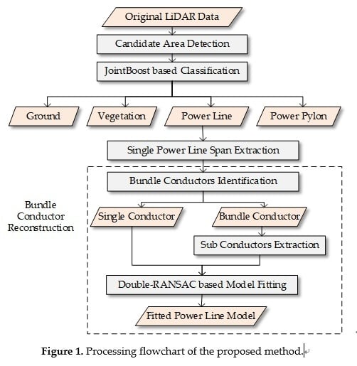
The processing flowchart of the proposed method is shown in Figure 1. First, points in the high-voltage power transmission corridors were detected by the Hough transformation and classified into four categories by a JointBoost classifier: ground, vegetation, power lines, and power pylons; second, for classified power lines, each single power line span was extracted by a spatial clustering-based method, and a fitting residual analyzing based method was introduced to identify bundle conductors from all power lines; third, a projected dichotomy method was adopted to extract each sub-conductor, on the XOY and XOZ planes, respectively; and finally, a double-RANSAC based model fitting algorithm was introduced to reconstruct each power line robustly and precisely.
1.3. Overview
The rest of the paper is organized as follows. Section 2 introduces a workflow for bundle conductor reconstruction. The experimental data and results are shown in Section 3 and Section 4, respectively. The robustness to noise and breakage of the proposed bundle conductor reconstruction method are discussed in Section 5. Finally, conclusions drawn from experiments are presented in Section 6.
2. Methodology
In this section, a JointBoost-based classification method for power transmission corridors and a spatial clustering method for single power line extraction are simply introduced in Section 2.1 and Section 2.2, respectively. Then, a fitting residual analyzing-based method for the identification of the bundle conductors is introduced in Section 2.3, and a projected dichotomy for sub-conductor extraction is introduced in Section 2.4. Finally, a double-RANSAC-based model fitting method is introduced in Section 2.5.
2.1. Power Transmission Corridor Detection and Classification
The real threat to the safety of power transmission lines are objects within a certain distance. However, during data acquisition, because of the flying height and the scanning angle of airborne LiDAR systems, a large number of non-interest points are usually acquired. To reduce the number of point clouds for subsequent processing, it is necessary to detect the candidate regions of the power transmission corridors first, and then to classify the points in the detected candidate regions.
According to the height characteristics of high-voltage power transmission corridors [18], the original point clouds are first converted to an elevation image to detect candidate regions by the Hough transformation [18,22]. Second, by referring to Guo et al.’s method [21], a JointBoost-based classification method was adopted with multiscale features [20,21,31] such as height features, surface features, eigen features, and density features, to classify points in candidate regions into four categories: ground, vegetation, power lines, and power pylons.
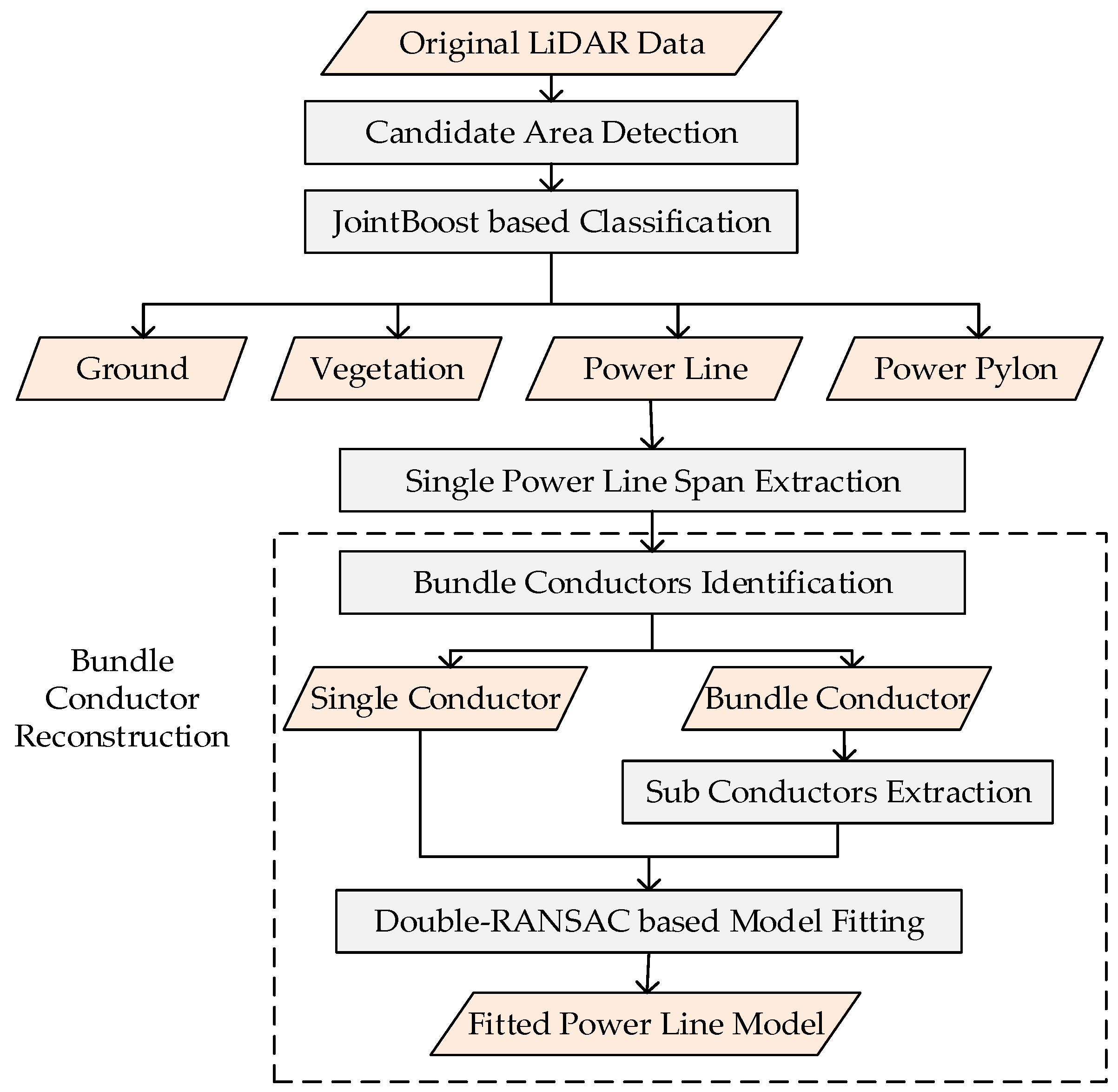
After the power lines between two power pylons were extracted, a local right-handed coordinate system was constructed. As shown in Figure 2, the lowest point of the power lines was defined as the origin, while the X-axis and Z-axis were parallel to the directions of the power lines and the height, respectively. It is worth noting that all following operations on the power lines were carried out on the local coordinate system.
2.2. Spatial Clustering-Based Single Power Line Span Extraction
Single power line span extraction is a basic step for precise bundle conductor extraction. As shown in Figure 3a, one obvious characteristic is that points in the same span are much closer than points in different spans. Since this was not the focus of this paper, by referring to the existing algorithm of Liang et al. [27], this paper extracted single power line spans by a spatial clustering method, according to their spatial distribution.
For line breaks, consistency checking was adopted based on the projected line equations. As shown in Figure 3b, first, the two breakage points A and B are located; then, considering that the same power line span appears as a straight line between two power pylons on the XOY plane, clustered power line spans are projected on the XOY plane to calculate their projected line equations by a least square algorithm [25]. Taking into account the situation of different spans in a vertical arrangement where the height differences of points in the same spans are much smaller than points in different spans, a height difference threshold Th is set. When the power lines satisfy the following conditions at the same time, the power lines are regarded as the same span and reconnected: (1) the slope and intercept differences of the two projected line equations are less than thresholds Tk and Tb, respectively; and (2) the height difference of the two points A and B is less than a threshold TH. According to the characteristics of power lines in high-voltage transmission corridors, in the experiments, we set the Tk = 0.05, Tb =1.5, and TH = 1 m.
2.3. Fitting Residuals-Based Bundle Conductor Identification
Identifying bundle conductors is the premise to extract each sub-conductor. The bundle conductor is a set of parallel conductors that are arranged on the vertices of regular symmetrical polygons [7]. Sub-conductors are spaced at a certain splitting diameter (0.2–0.5 m). Generally, for high-voltage transmission lines, the number of bundle conductors is not more than four. For example, as shown in Figure 4, the 220 kV high-voltage transmission lines are usually 2-bundled conductors (Figure 4a,b), while the 500 kV high-voltage transmission lines are 4-bundled conductors (Figure 4c).
According to the above features, theoretically, bundle conductors can be identified through the fitting residuals of single power line spans, since the fitting residuals of bundle conductors are large, while the fitting residuals of single conductors are small. Therefore, single power line span fitting is conducted first, then the fitting residuals from the original point to the nearest fitting point are calculated according to Equation (1). If the fitting residual of a single power line span is larger than a residual threshold TR (TR is generally half of the diameter), this power line is identified as a bundle conductor; otherwise, it is a single conductor.
where n is the number of points in a span; r(xi) is the distance from the original point to the nearest fitting point.
To distinguish the arrangement of bundle conductors, the fitting residuals in the XY direction and the Z direction are also respectively computed, according to Equation (1). For 2-bundled conductors, if the residual in the XY direction is much larger than the residual in the Z direction, it is in a horizontal arrangement; otherwise, it is in a vertical arrangement.
2.4. Projected Dichotomy for Sub-Conductor Extraction
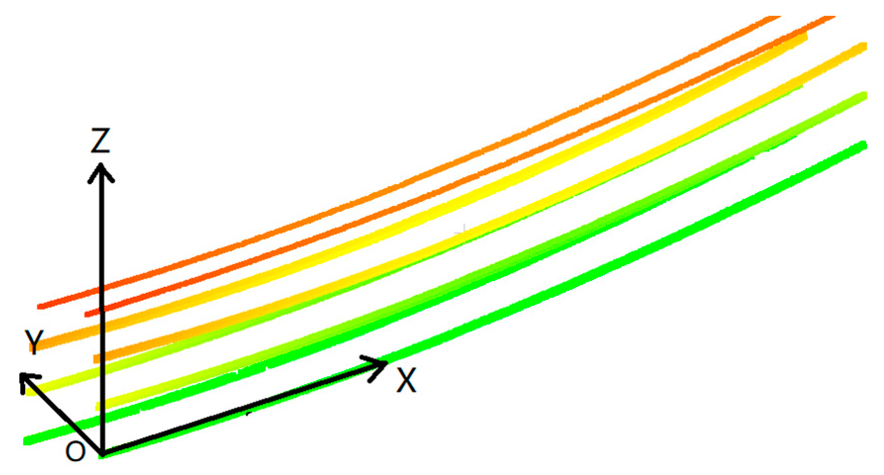
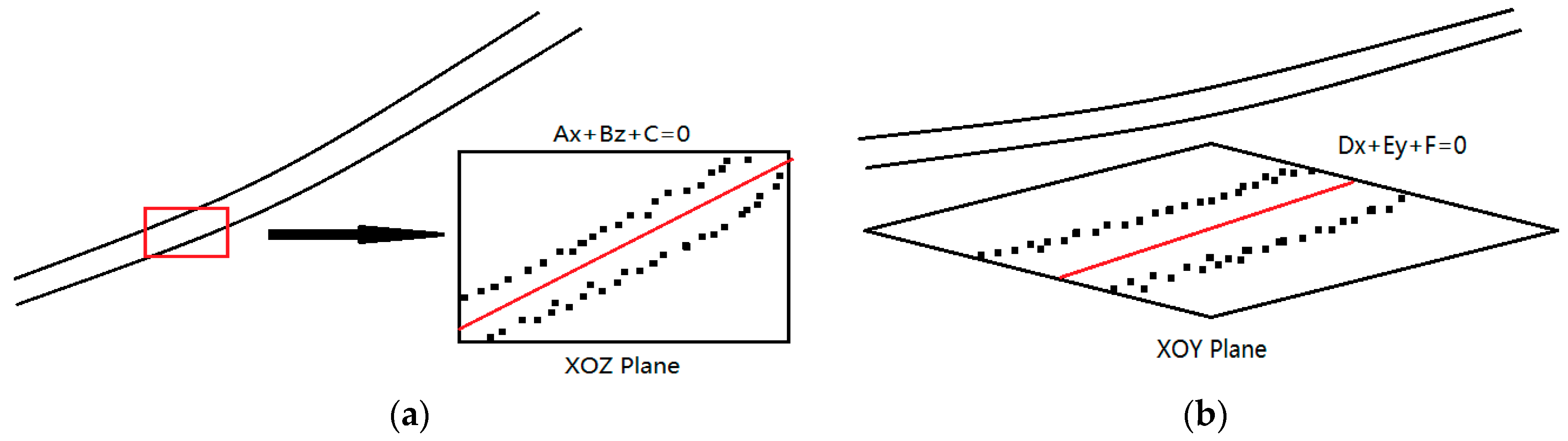
After a bundle conductor is identified, a projected dichotomy method is introduced for sub-conductor extraction. As shown in Figure 5, the projection dichotomy mainly includes the projections on two planes: the XOY plane and the XOZ plane.
Projected dichotomy on the XOZ plane: This step is mainly performed to divide a whole into two subsets: up and bottom. As shown in Figure 5a, point clouds of a single power line span are first divided into several segments, and then each segment is projected onto the XOZ plane. When their length is small enough, each sub-conductor in the segment can be considered as a straight line. Therefore, a least square-based line model fitting is first adopted for each segment to obtain a projected line equation Ax + Bz + C = 0 on the XOZ plane. Then, the distances for all points Dis_xoz in this segment are calculated according to Equation (2) and located according to Equation (3). If the distance Dis_xoz from the point to the projected line is larger than 0, it is assumed to be in the up of the section; otherwise, it is on the bottom.
Projected dichotomy on the XOY plane: This step is mainly performed to divide a whole into two subsets: left and right. As shown in Figure 5b, the whole point clouds of a single span is first projected onto the XOY plane, and then, similar to the XOZ plane projected dichotomy, a least square based-line model fitting is adopted to obtain the projected line equation Dx + Ey + F = 0 on the XOY plane. Finally, the distances of all points Dis_xoy are calculated according to Equation (4) and located according to Equation (5): If the distance Dis_xoy from the point to the projected line is larger than 0, it is assumed to be on the left of the section; otherwise, it is on the right.
For 2-bundled conductors, as mentioned in Section 2.3, there are two kind of arrangements: horizontal and vertical. If it is in a horizontal arrangement, a projected dichotomy only on the XOY plane is adopted to divide the bundle conductor into left and right subsets; otherwise, a projected dichotomy on the XOZ plane is adopted to divide it into up and bottom subsets. For 4-bundled conductors, a projected dichotomy on the XOZ plane is first conducted to divide them into two subsets: up and bottom, and then for each subset, a projected dichotomy on the XOZ plane is required respectively to extract each sub-conductor.
2.5. Double-RANSAC-Based Model Fitting
As mentioned in the literature reviews, most model fitting methods of power lines usually consist of two key parts: choosing a mathematical model and selecting the parameter estimation algorithm.
For model choosing, a 3D model can be decomposed into two parts: a 2D model on the XOY plane, and a 2D model on the XOZ plane [32]. Mathematical models such as parabola [27], piecewise line, and catenary [4,8,19,33,34] are mainly adopted for power line fitting. Since power lines between two adjacent pylons (i.e., over a span) have the shape of a catenary curve [1,33,34], thus, the 3D model used in this paper decomposed into two parts: a linear model on the XOY plane (Equation (6)) and a catenary model on the XOZ plane (Equation (7)):
where (x, y, z) is the coordinate of a power line point; a, b, k are the parameters to be solved; , , , and other parameters are defined as shown in Figure 6:
For parameter estimation, RANSAC [23,24] and least square [25] are two widely applied algorithms. The LS-based methods estimate parameters by minimizing the square error sum between the measured data and the modeled data, while RANSAC iteratively determines the optimal parameters from data containing a large number of outliers. As shown in Figure 7, the RANSAC algorithm iterates the following two steps [8]: (1) randomly generating a hypothesis; and (2) verifying the hypothesis by the remaining data. Given a set of seed points, the initial parameters of a model can be calculated, where a hypothesis is generated. Through iteration, the optimal parameters are solved. Since the LS algorithm is sensitive to noise, while RANSAC is much more robust, a double-RANSAC based method was used to fit the power line accurately, where RANSAC-based line fitting was used to fit power lines onto the XOY plane, and RANSAC-based catenary fitting was used to fit them on the XOZ plane.
The RANSAC-based catenary fitting algorithm on the XOZ plane first calculates the catenary model parameter k according to randomly generated points, then verifies its correctness by the remaining points. As shown in Figure 8, in the sub-step of the Initial Catenary Model Calculation, an iteration based on a least square algorithm was used to solve the unknown parameter k in the catenary equation. The detailed procedure is shown in Algorithm 1. The optimal parameter k is estimated by iteration, then the fitting points are calculated according to the optimal parameter k, with the aid of the start and end of the power line. The noise points can be effectively removed by calculating the distance from the original point to the nearest fitting point.
| Algorithm 1. Detailed procedure of initial catenary model calculation. |
|
The RANSAC-based line-fitting algorithm on the XOY plane was similar to that of the fitting process on the XOZ plane, and the only difference was the mathematical model, where the linear model (Equation (6)) was used instead of the catenary model (Equation (7)).
3. Experimental Data
To verify the feasibility of the proposed method, a set of experiments was conducted on three LiDAR datasets that were collected from different transmission lines in Guangdong Province, China. The original point clouds were collected by a Riegl VUX-1 laser measurement system.
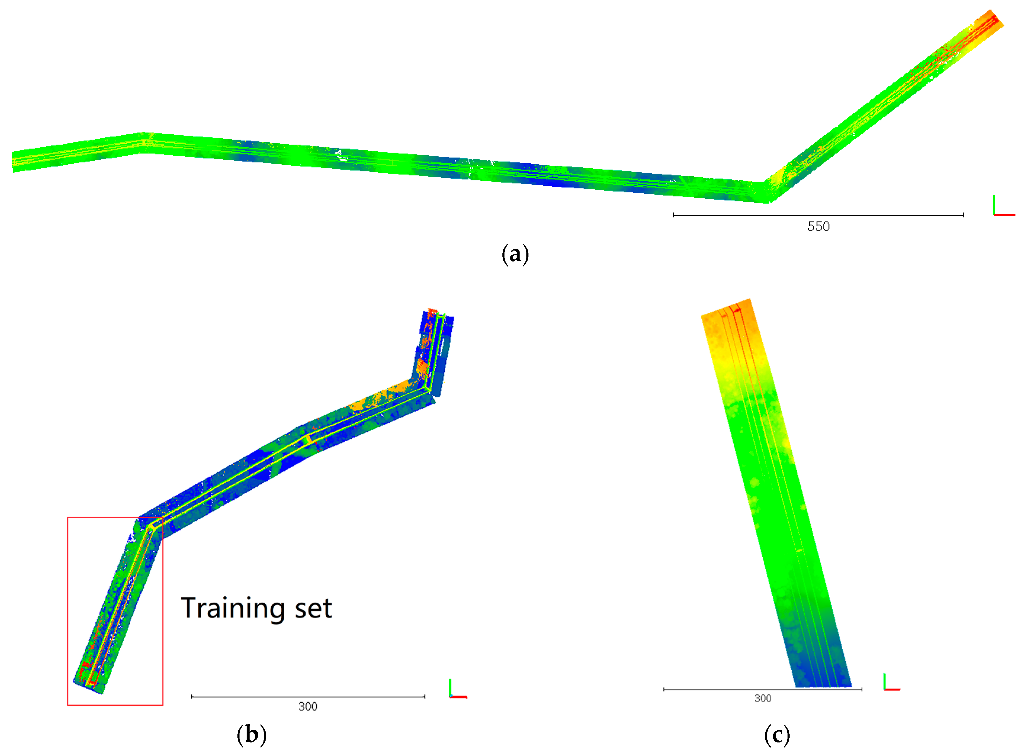
As mentioned in Section 2.1, to reduce the number of points for subsequent processing, the transmission corridors of three datasets were first detected. Although they were collected from the same scanner, the three datasets were quite different because of the differences in flying height, speed, and topography. Details about the three processed datasets are shown in Table 1, and their overviews are shown in Figure 9.
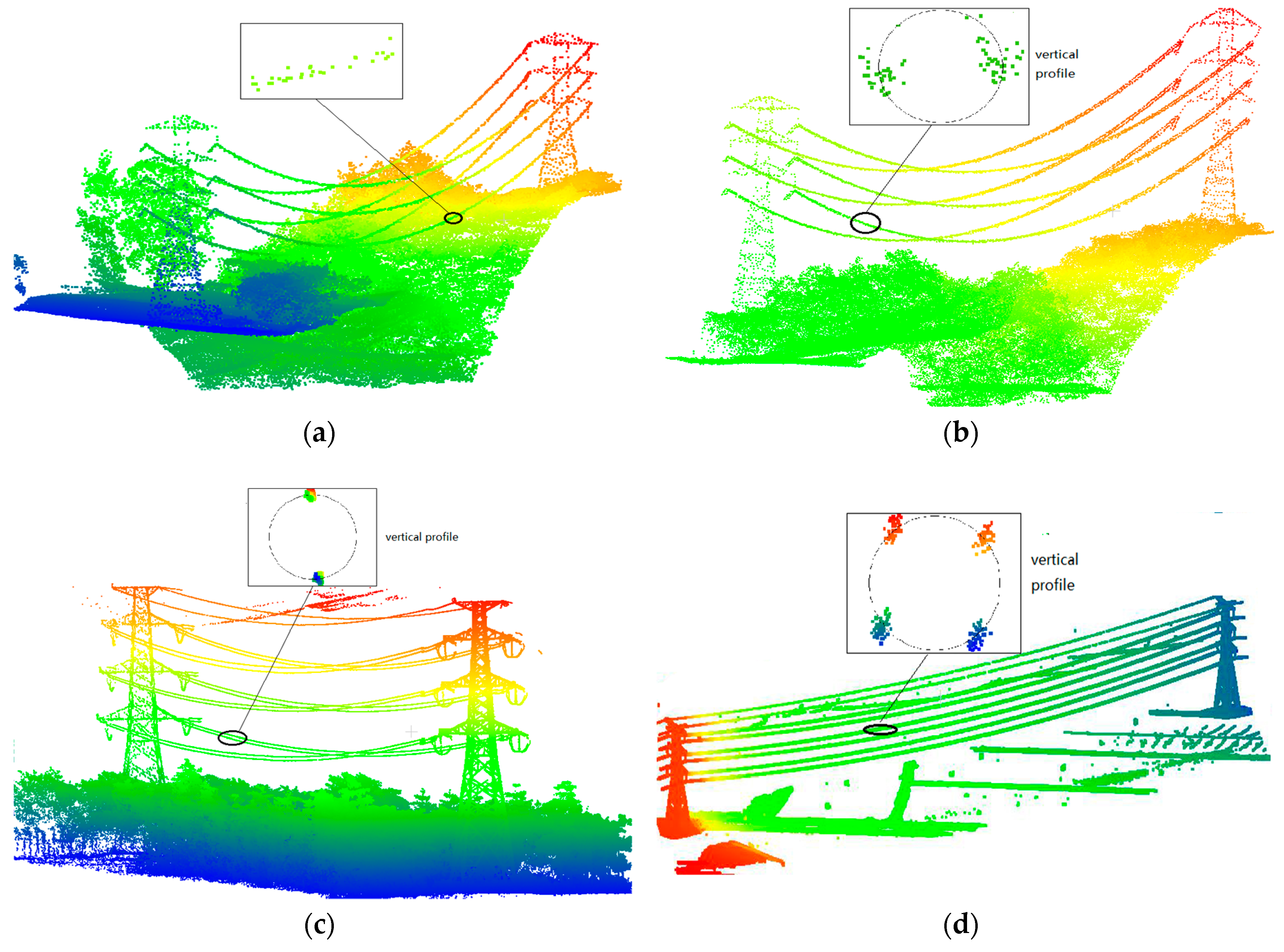
For high-voltage transmission corridors, as shown in Figure 10, there are four main objects: ground, vegetation, power lines, and power pylons. Inevitably, as shown in Figure 10c,d, there is some noise caused by external factors (such as light, vibration, noise, etc.) and the scanner itself during working. The above three datasets included four typical power lines in high-voltage transmission corridors: (1) single conductor (Figure 10a); (2) 2-bundled conductor in horizontal arrangement (Figure 10b); (3) 2-bundled conductor in vertical arrangement (Figure 10c); and (4) 4-bundled conductor (Figure 10d). In particular, there were two transmission lines that were located closely in Dataset III, which contained two kinds of power lines: a 2-bundled conductor in a horizontal arrangement, and a single conductor.
4. Results
In this section, experiments were conducted on the three datasets with the proposed method, and the results are shown as follows: the classification accuracy of the power transmission corridors based on a JointBoost classifier is first listed in Section 4.1; then, the accuracy of the bundle conductor identification is shown in Section 4.2; the sub-conductor extraction results are shown in Section 4.3; and the accuracy of power line model fitting is listed in Section 4.4.
4.1. Power Transmission Corridor Classification
To obtain the object distribution in high-voltage transmission corridors, a JointBoost-based method was adopted to classify points in the detected corridors into four categories: ground, vegetation, power lines, and power pylons. As shown in Figure 9b, the point clouds between the two power pylons in Dataset II were first selected as the training set, and manually labeled to train the JointBoost classifier model. Other data were regarded as the testing sets. Considering that the unbalanced distribution of training examples per class (especially power lines and power pylons) in the training set may often have a detrimental effect on the training process [35,36,37], this paper adopted a re-balancing strategy by repeating the training samples in small amounts to keep all samples in the same magnitude. The information of the training data is listed in Table 2. Typical classification results of the testing sets are shown in Figure 11.
It can be seen from the Figure 11 that the continuous vegetation and isolated vegetation are basically classified correctly, and the distribution of power lines, power pylons, and ground points are generally in accordance with the actual situation. However, there are still some misclassifications, for example, due to the local features’ similarity between vegetation and the power pylons at the bottom, some points at the bottom of the power pylons are misclassified as vegetation.
To quantitatively evaluate the accuracy of the classified results, the point clouds in dataset II are all manually classified as reference, and the three-point accuracy evaluation method, Precise, Recall and Overall Accuracy [8,38] are adopted. As shown in Table 3, the vegetation and power lines have both high precision and recall, which satisfy the requirements of vegetation monitoring and power line monitoring.
4.2. Bundle Conductor Identification
To verify the proposed fitting residual-based bundle conductor identification method, experiments are conducted on 73 classified power lines (25 lines in dataset I, 24 lines in dataset II, and 24 lines in dataset III). The identification results are shown in Table 4, where the fitting residual threshold TR is set to 0.2 m in this paper.
As shown in Table 4, most of the bundle conductors were correctly identified according to the fitting residual analysis, while two single conductors in Dataset III were misidentified as 2-bundled conductors. This was due to the low point density and low data quality. As shown in Figure 12, when the point density and data quality were high, the shape of the power line was more regular and more in accordance with the catenary (Figure 12a); when the point density and data quality were low, the points of power lines were more discrete (Figure 12b), leading the fitting residual to be much higher, and then misidentification always occurred.
To obtain a better understanding of the fitting residual of different power lines, the fitting residuals of four typical power lines were listed in Table 5, Table 6, Table 7 and Table 8, respectively. Additionally, the fitting residuals in the XY direction and Z direction were calculated to explore the relationship between their arrangements and their fitting residuals. It can be seen clearly that, for the single conductors, their fitting residuals in all directions were very small; for 2-bundled conductors, their fitting residuals in the splitting direction were much larger than the others; and for 4-bundled conductors, which can be regarded as splitting in both directions, all fitting residuals were large. This shows that the fitting residual analysis-based method is suitable for most situations with high point density and high data quality to identify bundle conductors.
4.3. Sub-Conductor Extraction
As mentioned in Section 2.3, the bundle conductor is a set of parallel conductors where sub-conductors are spaced at a certain diameter and arranged on the vertices of regular symmetrical polygons. According to these features, a projected dichotomy method was proposed for sub-conductor extraction. To verify the proposed method, experiments were conducted on all bundle conductors. The extraction results are shown in Table 9.
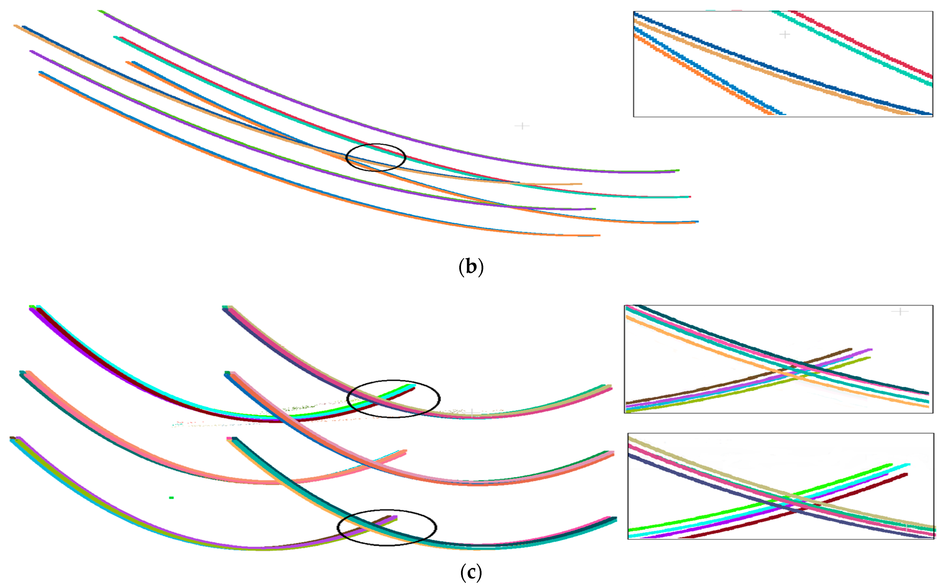
In this experiment, all bundle conductors with various arrangements and bundle numbers in the three datasets were correctly extracted. To visually check the extraction results of the sub-conductors, three typical results are shown in Figure 13, and each sub-conductor is colored differently to easily distinguish them. Although residing very close together, each sub-conductor was still well extracted effectively through this method.
It is worth noting that, for 2-bundled conductors, as mentioned in Section 2.3, a projected dichotomy on only one plane was adopted, according to their arrangement. For 4-bundled conductors, the projected dichotomy on the both XOY and XOZ plane were conducted, respectively.
4.4. Power Line Model Fitting
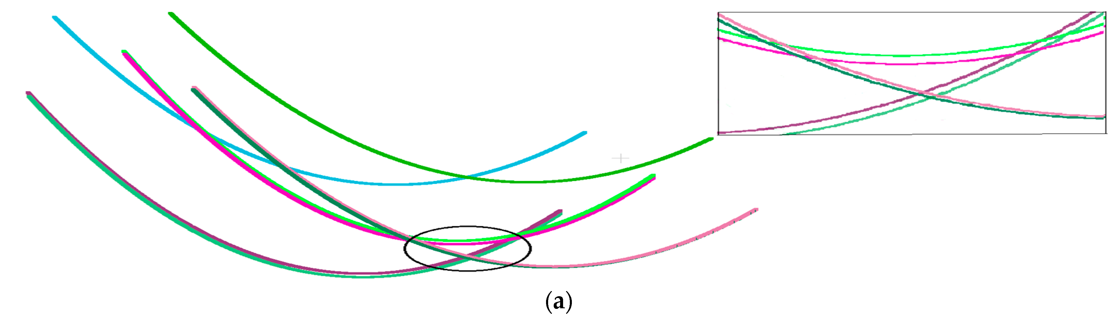
In this section, a double-RANSAC based method was proposed to fit the extracted power lines. All power lines in the three datasets were tested. Typical results are shown in Figure 14, where each of the fitted power lines is colored in a different color. It can be seen that the fitted power lines were parallel and disjointed, basically consistent with the distribution of the power lines.
To give a quantitative precision of the fitted power line model, the fitting residuals defined in Section 2.3 were calculated. The experiment showed that, after sub-conductor extraction, the fitting residuals of most power lines were less than 0.2 m. To compare the difference between the single power line span fitting and sub-conductor fitting, the fitting residual of the single power line span D_sum, and the residual of each sub-conductor D_sub were calculated. Three examples are listed in Table 10. It was found that the fitting residuals of each sub-conductor were smaller than 1/n of the whole span’s fitting residuals, where n is the splitting number.
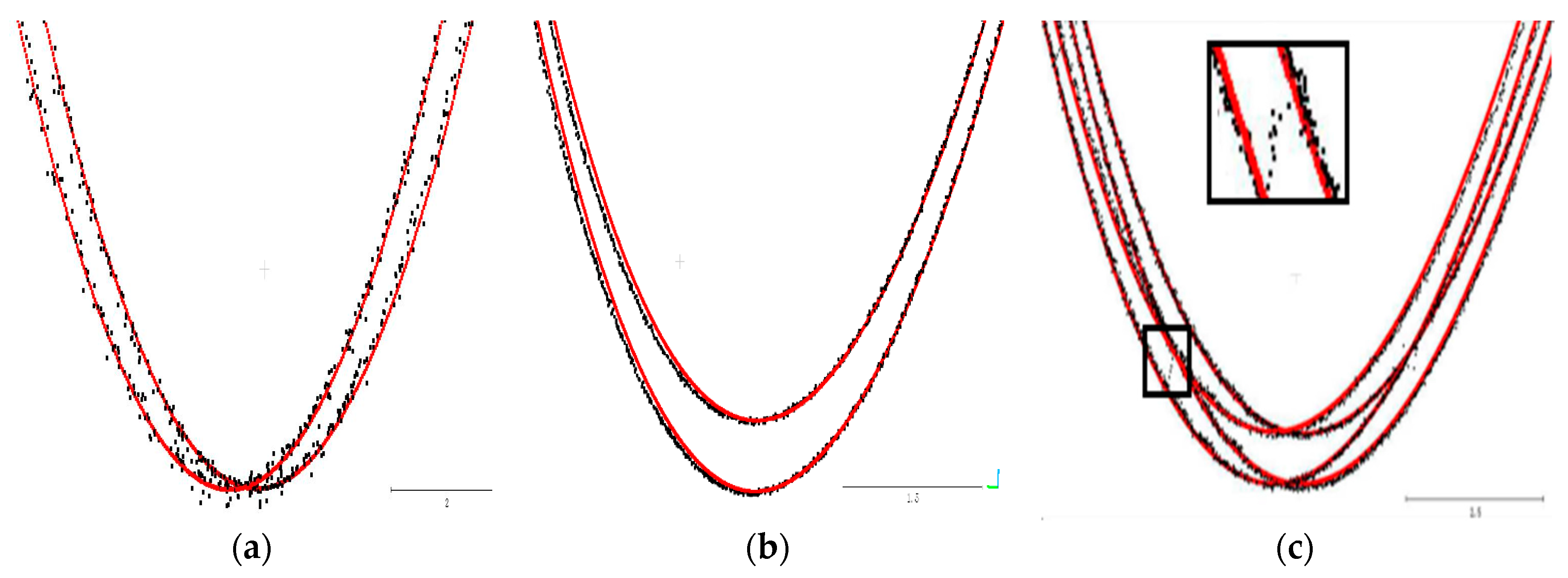
For direct comparison, three typical fitted power lines were magnified and overlaid with original points in Figure 15, where the fitted models are colored in red and the original points are colored in black. Through the comparison, it shows that even if there were spacers in the bundle conductor (Figure 15c), the projected dichotomy could still work to accurately extract each sub-conductor, and the power lines were accurately fitted by the double-RANSAC fitting method.
5. Discussion
In this section, the robustness to noise and the breakage of the proposed method is discussed. The robustness to noise, which is mostly due to the double-RANSAC-based model fitting method, is discussed in Section 5.1, and the robustness to breakage, which is thanks to the projected dichotomy-based extraction method, is discussed in Section 5.2; and the effect of data quality is quantitatively analyzed in Section 5.3.
5.1. Robustness to Noise
In data acquisition, which is affected by external factors (such as light, vibration, noise, etc.) and the scanner itself, there is inevitably some noise. As shown in Figure 16a, there was a large continuous noise across the two power line spans, which caused additional difficulty for model fitting with high precision. However, through the proposed double-RANSAC based model fitting method, noise could be efficiently removed (Figure 16b), and the fitting results were mostly in accordance with the power lines’ distribution, which were not badly affected by noise.
This is mainly due to the advance of the RANSAC algorithm: on the XOY plane, power lines are linear, and the effect of noise can be reduced when calculating the optimal linear model by RANSAC, resulting in the linear model being basically in accordance with the linear characteristics of the power line; on the XOZ plane, the power line’s catenary characteristics are obvious. When calculating the optimal catenary model, the influence of noise points can be minimized or avoided as much as possible, so that the parameters basically conform to the catenary characteristics of the power line.
Additionally, most noise can be removed by calculating the fitting residual from the original point to the nearest fitting point. As the residual between the power line point and the fitting point is generally small, while the residual between the noise point and the fitting point is large, the noise points can be eliminated effectively.
5.2. Robustness to Breakage
Sparseness and large gaps often occur when a section of power line is obscured by vegetation or lacks data points, leading to a small number of power lines being split into several parts, or being undetected [8]. To analyze the robustness to breakage, a set of experiments were conducted by the proposed method.
Taking a 2-bundled conductor in a vertical arrangement as an example, as shown in Figure 17, there was a large breakage of the 2-bundled conductor, where both sub-conductors disappeared. Through a projected dichotomy on the XOZ plane, the power lines were divided into several parts and projected onto the XOZ plane (Figure 17a), then each sub-conductor was extracted (Figure 17b). The fitting result of the broken bundle conductor is shown in Figure 17c, and shows that the proposed method could efficiently reduce the impact of breakage.
This also works for breakages where single sub-conductors have been removed. As shown in Figure 18a, only one sub-conductor of a single span was removed. Although the points in the breakage section were wrongly extracted (red box in Figure 18b), each sub-conductor was still well modeled through a double-RANSAC-based model fitting method (Figure 18c). Thus, it shows that the proposed bundle conductor reconstruction method has a high fault-tolerant capability.
5.3. Effect of Data Quality
As mentioned in Section 4.2, misidentifications always occur when the point density or data quality is low. To quantitatively analyze the impact of the data quality required for the successful bundle conductor extraction and reconstruction, a set of experiments was conducted by controlling the degradation of high quality data.
As shown in Figure 19, we selected power lines between two power pylons with high data quality as the original data. The power lines included six 2-bundled conductors in a vertical arrangement, and two single conductors. The splitting diameter of the six 2-bundled conductor was about 0.7 m. There was little noise and breakage, and the point distance was about 0.2 m.
To explore the effect of difference point distances and Gaussian noise, we respectively sampled the original power lines and added Gaussian noise, and then the bundle conductor extraction and reconstruction were conducted on the processed data. Table 11 and Table 12 list the results of different sample distances and Gaussian noise, where Success is the number of correctly reconstructed power lines, Failure is the number of wrongly reconstructed power lines, and mr is the sample distance.
Table 11 shows that as the sample distance increased from 0.2 m to 0.6 m, the power lines were still correctly reconstructed. When the sample distance was up to 0.7 m, misidentification occurred, and two 2-bundled conductors were misclassified as single conductors. Then, the larger the sample distance, the higher the Failure rate.
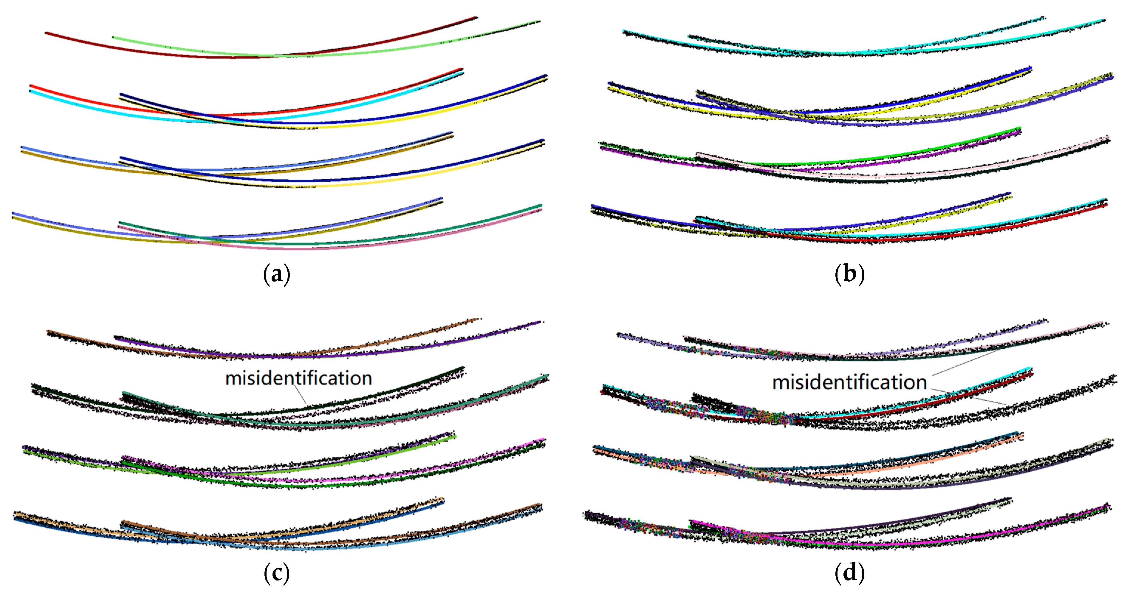
Table 12 shows that as the standard deviation of Gaussian noise increased from 0.1 mr to 0.6 mr, the proposed method could still work well, which indicates its robustness to noise. However, when the deviation was up to 0.7 mr or larger, misidentification occurred: (1) the vertical arrangement was misidentified as the horizontal arrangement; (2) 2-bundled conductors were misclassified as single conductors; and (3) single conductors were misrecognized as bundled conductors. Typical results of different Gaussian noise are shown in Figure 20.
Experiments showed that the extraction and reconstruction of bundle conductors relies highly on the point density and data quality. The larger the sample distance, the less obvious the bundle conductor feature. Additionally, the thresholds of the sample distances are related to the splitting diameters of the bundle conductors. The experiments suggest that for good reconstruction, the point distance should be smaller than the splitting diameters. As for noise, the proposed method has a high robustness to noise. However, if noise increases, the points of the power lines will be more discrete, and the shapes of the bundle conductors will be indistinct, consequently leading to misidentification.
6. Conclusions
For the inspection of power transmission lines, power lines are the focus of hazard detection (e.g., vegetation monitoring and power line monitoring), and its reconstruction has received much attention. A robust and precise power line model is a necessary requirement for rapid and correct clearance in cases of potential hazards. However, most of the existing research has only focused on single power line span reconstruction, and limited methods have been reported for bundle conductor reconstruction. Thus, this paper proposed a novel method for high-voltage power line reconstruction, which could precisely reconstruct each sub-conductor. After a single power line span was extracted, and each bundle conductor was first identified by analyzing their fitting residuals; then, each sub-conductor of each bundle conductor was extracted by a projected dichotomy method on the XOY and XOZ planes, respectively; finally, a double-RANSAC-based algorithm was introduced to reconstruct each line.
The proposed reconstruction method has several merits: (1) the structure characteristics of bundle conductors in high-voltage transmission corridors are used for their identification and extraction; (2) the proposed projected dichotomy method can efficiently and precisely extract each sub-conductor, and is robust to noise and breakage; and (3) the double-RANSAC based model fitting method can reduce the effect of continuous noise. Overall, the proposed method can preferably reconstruct the real structure of bundle conductors robustly, with a high precision of better than 0.2 m. Additionally, with the classified power transmission and well-reconstructed power lines, related applications such as vegetation monitoring and power line monitoring can be conducted.
It is worth noting that the reconstruction of bundle conductors relies highly on the point density and data quality. Errors always occur when points are sparse and their structure is not apparent. In our future work, for better power transmission inspection and management, the power line reconstruction results will be combined with reconstructed power pylons to add contextual information. As the distribution of high-voltage transmission lines is becoming more complicated (e.g., multi-loop and multi-bundle), more attention will be paid on more applicable and general 3D methods for bundle conductor reconstruction. Due to the limited research that is reported for bundle conductor reconstruction, our work may inspire more researchers to work in this field and to achieve better results.
Author Contributions
Conceptualization, W.J. and R.Z.; Methodology, R.Z.; Validation, W.J., R.Z. and S.J.; Formal Analysis, R.Z.; Investigation, W.J.; Resources, W.J. and R.Z.; Data Curation, W.J.; Writing-Original Draft Preparation, R.Z.; Writing-Review & Editing, R.Z. and S.J.; Supervision, W.J. and S.J.; Project Administration, W.J.; Funding Acquisition, W.J.
Funding
This research was funded by the Key Technology Program of China South Power Grid grant number GDKJQQ20161187.
Acknowledgments
The authors would like to express their gratitude to the editors and the reviewers for their constructive and helpful comments for the substantial improvement of this paper. The dataset was provided by the patrol operation center of Guangdong Power Grid Co. Ltd.
Conflicts of Interest
The authors declare no conflict of interest.
References
- Matikainen, L.; Lehtomäki, M.; Ahokas, E.; Hyyppä, J.; Karjalainen, M.; Jaakkola, A.; Kukko, A.; Heinonen, T. Remote sensing methods for power line corridor surveys. ISPRS J. Photogramm. Remote Sens. 2016, 119, 10–31. [Google Scholar] [CrossRef]
- Zhou, R.; Jiang, W.; Huang, W.; Xu, B.; Jiang, S. A Heuristic Method for Power Pylon Reconstruction from Airborne LiDAR Data. Remote Sens. 2017, 9, 1172. [Google Scholar] [CrossRef]
- Global Transmission and Distribution Report—Infrastructure, Upcoming Projects, Investments, Key Operators and Analysis to 2020. Available online: https://www.globaldata.com/store/search/power/ (accessed on 20 July 2017).
- Qin, X.; Wu, G.; Ye, X.; Huang, L.; Lei, J. A Novel Method to Reconstruct Overhead High-Voltage Power Lines Using Cable Inspection Robot LiDAR Data. Remote Sens. 2017, 9, 753. [Google Scholar] [CrossRef]
- Aggarwal, R.K.; Johns, A.T.; Jayasinghe, J.A.S.B.; Su, W. An overview of the condition monitoring of overhead lines. Electr. Power Syst. Res. 2000, 53, 15–22. [Google Scholar] [CrossRef]
- Torabzadeh, H.; Morsdorf, F.; Schaepman, M.E. Fusion of imaging spectroscopy and airborne laser scanning data for characterization of forest ecosystems—A review. ISPRS J. Photogramm. Remote Sens. 2014, 97, 25–35. [Google Scholar] [CrossRef]
- Yang, J.; Kang, Z. Voxel-Based Extraction of Transmission Lines from Airborne LiDAR Point Cloud Data. IEEE J. Sel. Top. Appl. Earth Obs. Remote Sens. 2018, 11, 1–13. [Google Scholar] [CrossRef]
- Guo, B.; Li, Q.; Huang, X.; Wang, C. An improved method for power-line reconstruction from point cloud data. Remote Sens. 2016, 8, 36. [Google Scholar] [CrossRef]
- Qin, X.; Wu, G.; Lei, J.; Fan, F.; Ye, X. Detecting Inspection Objects of Power Line from Cable Inspection Robot LiDAR Data. Sensors (Basel) 2018, 18, 1284. [Google Scholar] [CrossRef]
- Mills, S.J.; Castro, M.P.G.; Li, Z.; Cai, J.; Member, S.; Hayward, R.; Mejias, L.; Walker, R.A. Evaluation of Aerial Remote Sensing Techniques for Vegetation Management in Power-Line Corridors. IEEE Trans. Geosci. Remote Sens. 2010, 48, 3379–3390. [Google Scholar] [CrossRef] [Green Version]
- Bartholomew, N.R.; Burdett, J.M.; Vandenbrooks, J.M.; Quinlan, M.C.; Call, G.B. Impaired climbing and flight behaviour in Drosophila melanogaster following carbon dioxide anaesthesia. Sci. Rep. 2015, 5, 339–352. [Google Scholar] [CrossRef]
- Sarabandi, K.; Park, M. Extraction of Power Line Maps from Millimeter-Wave Polarimetric SAR Images. IEEE Trans. Antennas Propag. 2000, 48, 1802–1809. [Google Scholar] [CrossRef]
- Stockton, G.R. Advances in applications and methodology for aerial infrared thermography. Proc. SPIE Int. Soc. Opt. Eng. 2004, 6205, 124. [Google Scholar] [CrossRef]
- Li, Z.; Liu, Y.; Walker, R.; Hayward, R.; Zhang, J. Toward automatic power line detection for a UAV surveillance system using pulse coupled neural filter and an improved hough transform. Mach. Vis. Appl. 2010, 21, 677–686. [Google Scholar] [CrossRef]
- Jiang, S.; Jiang, W.; Huang, W.; Yang, L. UAV-based oblique photogrammetry for outdoor data acquisition and offsite visual inspection of transmission line. Remote Sens. 2017, 9, 278. [Google Scholar] [CrossRef]
- Xiang, Q.; Li, J.; Wen, C.; Huang, P. Extraction of power lines from mobile laser scanning data. Proc. SPIE 2016, 9901, 990105. [Google Scholar] [CrossRef]
- Cheng, L.; Tong, L.; Wang, Y.; Li, M. Extraction of Urban Power Lines from Vehicle-Borne LiDAR Data. Remote Sens. 2014, 6, 3302–3320. [Google Scholar] [CrossRef] [Green Version]
- Zhu, L.; Hyyppä, J. Fully-automated power line extraction from airborne laser scanning point clouds in forest areas. Remote Sens. 2014, 6, 11267–11282. [Google Scholar] [CrossRef]
- McLaughlin, R.A. Extracting transmission lines from airborne LIDAR data. IEEE Geosci. Remote Sens. Lett. 2006, 3, 222–226. [Google Scholar] [CrossRef]
- Kim, H.B.; Sohn, G. Point-based Classification of Power Line Corridor Scene Using Random Forests. Photogramm. Eng. Remote Sens. 2013, 79, 821–833. [Google Scholar] [CrossRef]
- Guo, B.; Huang, X.; Zhang, F.; Sohn, G. Classification of airborne laser scanning data using JointBoost. ISPRS J. Photogramm. Remote Sens. 2015, 100, 71–83. [Google Scholar] [CrossRef]
- Wang, Y.; Chen, Q.; Liu, L.; Zheng, D.; Li, C.; Li, K. Supervised classification of power lines from airborne LiDAR data in Urban Areas. Remote Sens. 2017, 9, 771. [Google Scholar] [CrossRef]
- Choi, S.; Kim, T.; Yu, W. Performance evaluation of RANSAC family. In Proceedings of the British Machine Vision Conference, London, UK, 7–10 September 2009. [Google Scholar]
- Chum, O.; Matas, J. Optimal randomized RANSAC. IEEE Trans. Pattern Anal. Mach. Intell. 2008, 30, 1472–1482. [Google Scholar] [CrossRef] [PubMed]
- Stigler, S.M. Gauss and the Invention of Least Squares. Ann. Stat. 1981, 9, 465–474. [Google Scholar] [CrossRef]
- Melzer, T.; Briese, C. Extraction and Modeling of Power Lines from ALS Point Clouds. In Proceedings of the 28th Work Austrian Association Pattern Recognition, Hagenberg, Austria, 17–18 June 2004; Volume 8. [Google Scholar]
- Liang, J.; Zhang, J. A New Power-line Extraction Method Based on Airborne LiDAR Point Cloud Data. Int. Symp. Image Data Fusion 2011, 2–5. [Google Scholar] [CrossRef]
- Chen, Z.; Lan, Z.; Long, H.; Hu, Q. 3D modeling of pylon from airborne LiDAR data. In Proceedings of the SPIE 9158, Remote Sensing of the Environment: 18th National Symposium on Remote Sensing of China, 915807, Wuhan, China, 20–23 October 2012. [Google Scholar]
- Li, Q.; Chen, Z.; Hu, Q. A model-driven approach for 3d modeling of pylon from airborne LiDAR data. Remote Sens. 2015, 7, 11501–11524. [Google Scholar] [CrossRef]
- Guo, B.; Huang, X.; Li, Q. A Stochastic Geometry Method for Pylon Reconstruction from Airborne LiDAR Data. Remote Sens. 2016, 8, 243. [Google Scholar] [CrossRef]
- Blomley, R.; Jutzi, B.; Weinmann, M. Classification of Airborne Laser Scanning Data Using Geometric Multi-Scale Features and Different Neighbourhood Types. ISPRS Ann. Photogramm. Remote Sens. Spat. Inf. Sci. 2016, III-3, 169–176. [Google Scholar] [CrossRef]
- Chen, C.; Yang, B.; Song, S.; Peng, X.; Huang, R. Automatic clearance anomaly detection for transmission line corridors utilizing UAV-Borne LIDAR data. Remote Sens. 2018, 10, 613. [Google Scholar] [CrossRef]
- Guan, H.; Yu, Y.; Li, J.; Ji, Z.; Zhang, Q. Extraction of power-transmission lines from vehicle-borne lidar data. Int. J. Remote Sens. 2016, 37, 229–247. [Google Scholar] [CrossRef]
- Jwa, Y.; Sohn, G. A piecewise catenary curve model growing for 3D power line reconstruction. Photogramm. Eng. Remote Sens. 2015, 78, 1227–1240. [Google Scholar] [CrossRef]
- Chen, C.; Breiman, L. Using Random Forest to Learn Imbalanced Data; Technical Report 666; University of California, Berkeley: Berkeley, CA, USA, 2004. [Google Scholar]
- Weinmann, M.; Jutzi, B.; Hinz, S.; Mallet, C. Semantic point cloud interpretation based on optimal neighborhoods, relevant features and efficient classifiers. ISPRS J. Photogramm. Remote Sens. 2015, 105, 286–304. [Google Scholar] [CrossRef]
- Yang, Z.; Jiang, W.; Xu, B.; Zhu, Q.; Jiang, S.; Huang, W. A convolutional neural network-based 3D semantic labeling method for ALS point clouds. Remote Sens. 2017, 9, 936. [Google Scholar] [CrossRef]
- Yang, B.; Dong, Z.; Liu, Y.; Liang, F.; Wang, Y. Computing multiple aggregation levels and contextual features for road facilities recognition using mobile laser scanning data. ISPRS J. Photogramm. Remote Sens. 2017, 126, 180–194. [Google Scholar] [CrossRef]
Figure 1.
Processing flowchart of the proposed method.

Figure 2.
Local right-handed coordinate system.

Figure 3.
Extraction single power line span: (a) spatial clustering; and (b) consistency checking.

Figure 4.
Structure of three typical bundle conductors: (a) and (b) are a 2-bundled conductor in the horizontal arrangement and vertical arrangement, respectively; and (c) is a 4-bundled conductor.
Figure 4.
Structure of three typical bundle conductors: (a) and (b) are a 2-bundled conductor in the horizontal arrangement and vertical arrangement, respectively; and (c) is a 4-bundled conductor.

Figure 5.
Sub-conductor extraction: (a) projected dichotomy on the XOZ plane; and (b) projected dichotomy on the XOY plane.
Figure 5.
Sub-conductor extraction: (a) projected dichotomy on the XOZ plane; and (b) projected dichotomy on the XOY plane.

Figure 6.
Diagram of the catenary equation parameter.

Figure 7.
Flowchart of the RANSAC algorithm.

Figure 8.
Calculation of the initial catenary model.

Figure 9.
Airborne LiDAR (Light Detection and Ranging) data of the three processed datasets. (a–c) are the three detected high-voltage power transmission corridors of datasets I–III, respectively.
Figure 9.
Airborne LiDAR (Light Detection and Ranging) data of the three processed datasets. (a–c) are the three detected high-voltage power transmission corridors of datasets I–III, respectively.

Figure 10.
Original point clouds of four typical power lines. (a) single conductor; (b) 2-bundled conductor in a horizontal arrangement; (c) 2-bundled conductor in a vertical arrangement; and (d) 4-bundled conductor.
Figure 10.
Original point clouds of four typical power lines. (a) single conductor; (b) 2-bundled conductor in a horizontal arrangement; (c) 2-bundled conductor in a vertical arrangement; and (d) 4-bundled conductor.

Figure 11.
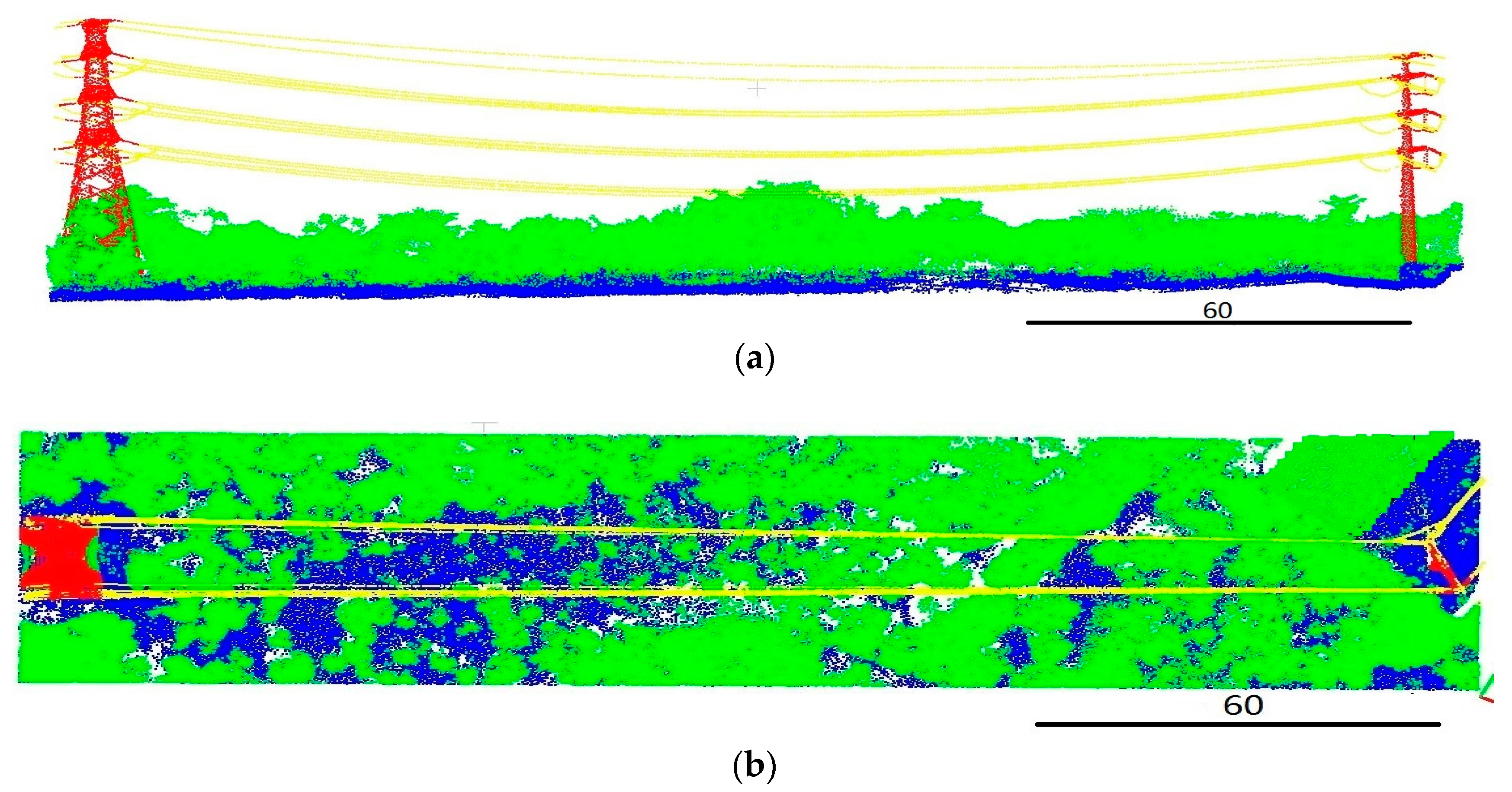
Power transmission corridor classification results. (a) front view; (b) vertical view. Ground points are colored in blue, vegetation points are colored in green, power lines are colored in yellow, and power pylons are colored in red.
Figure 11.
Power transmission corridor classification results. (a) front view; (b) vertical view. Ground points are colored in blue, vegetation points are colored in green, power lines are colored in yellow, and power pylons are colored in red.

Figure 12.
Original point clouds of single conductors. (a) is the correctly identified single conductor of high point density and high data quality, while (b) is the misidentified single conductor of low point density and low data quality.
Figure 12.
Original point clouds of single conductors. (a) is the correctly identified single conductor of high point density and high data quality, while (b) is the misidentified single conductor of low point density and low data quality.

Figure 13.
Results of the bundle conductor extraction. (a–c) are the extraction results of 2-bundled conductors in a horizontal arrangement; 2-bundled conductors in a vertical arrangement; and 4-bundled conductors, respectively.
Figure 13.
Results of the bundle conductor extraction. (a–c) are the extraction results of 2-bundled conductors in a horizontal arrangement; 2-bundled conductors in a vertical arrangement; and 4-bundled conductors, respectively.


Figure 14.
Model fitting results of power lines. (a–c) are the fitting results of the 2-bundled conductors in a horizontal arrangement, 2-bundled conductors in a vertical arrangement, and 4-bundled conductors, respectively.
Figure 14.
Model fitting results of power lines. (a–c) are the fitting results of the 2-bundled conductors in a horizontal arrangement, 2-bundled conductors in a vertical arrangement, and 4-bundled conductors, respectively.


Figure 15.
Comparison between the fitted power lines and the original points: (a) comparison of a 2-bundled conductor with a horizontal arrangement; (b) comparison of a 2-bundled conductor with a vertical arrangement; and (c) comparison of a 4-bundled conductor.
Figure 15.
Comparison between the fitted power lines and the original points: (a) comparison of a 2-bundled conductor with a horizontal arrangement; (b) comparison of a 2-bundled conductor with a vertical arrangement; and (c) comparison of a 4-bundled conductor.

Figure 16.
Robustness to noise: (a) the original power line points with noise; (b) bundle conductor extraction results; and (c) the double-RANSAC-based fitting results.
Figure 16.
Robustness to noise: (a) the original power line points with noise; (b) bundle conductor extraction results; and (c) the double-RANSAC-based fitting results.


Figure 17.
Robustness to breakage with both sub-conductors removed: (a) the original break power line; (b) sub-conductor extraction results; and (c) the double-RANSAC-based fitting results.
Figure 17.
Robustness to breakage with both sub-conductors removed: (a) the original break power line; (b) sub-conductor extraction results; and (c) the double-RANSAC-based fitting results.

Figure 18.
Robustness to breakage with single sub-conductors removed: (a) the original break power line; (b) sub-conductor extraction results; and (c) the double-RANSAC-based fitting results.
Figure 18.
Robustness to breakage with single sub-conductors removed: (a) the original break power line; (b) sub-conductor extraction results; and (c) the double-RANSAC-based fitting results.

Figure 19.
Original point clouds of power lines with high data quality.

Figure 20.
Effect of Gaussian noise. (a–d) are the Gaussian standard deviation = 0.3 mr, 0.5 mr, 0.7 mr, and 0.8 mr, respectively.
Figure 20.
Effect of Gaussian noise. (a–d) are the Gaussian standard deviation = 0.3 mr, 0.5 mr, 0.7 mr, and 0.8 mr, respectively.


Table 1.
Details of the three processed datasets.
| Dataset | Points Number | Area (m2) | Density (pts/m2) | Point Distance (m) | Line Number | Data Quality | Bundle Conductor Arrangement | |
|---|---|---|---|---|---|---|---|---|
| Along | Vertical | |||||||
| I | 43,879,821 | 40 ∗ 2000 | 548.5 | 0.10 | 0.35 | 25 | middle | 2-bundled in vertical |
| II | 25,212,971 | 40 ∗ 730 | 863.5 | 0.07 | 0.15 | 24 | high | 4-bundled conductor |
| III | 459,709 | 80 ∗ 600 | 9.6 | 0.45 | 0.50 | 24 | low | 2-bundled in horizontal; single conductor |
Table 2.
Information of training data.
| Type | Ground | Vegetation | Power Line | Power Pylon |
|---|---|---|---|---|
| Points number | 64,157 | 164,949 | 8507 | 6120 |
| Repeat number | 2 | 1 | 19 | 26 |
Table 3.
Classification accuracy of Dataset II.
| Overall Accuracy: 97.71% | ||||
|---|---|---|---|---|
| Ground | Vegetation | Power Line | Power Pylon | |
| Precision (%) | 99.35 | 97.40 | 97.02 | 94.35 |
| Recall (%) | 95.09 | 99.81 | 98.17 | 86.17 |
Table 4.
Bundle conductor identification.
| Single Conductor | 2-Bundled Conductor | 4-Bundled Conductor | ||
|---|---|---|---|---|
| Horizontal | Vertical | |||
| Total | 34 | 12 | 21 | 16 |
| Identified | 32 | 12 | 21 | 16 |
| Correctness | 94.17% | 100% | 100% | 100% |
Table 5.
Fitting residuals of single conductors.
| Residual | 1 | 2 | 3 | 4 | 5 | 6 |
|---|---|---|---|---|---|---|
| XY (m) | 0.04 | 0.03 | 0.05 | 0.05 | 0.06 | 0.07 |
| Z (m) | 0.02 | 0.04 | 0.07 | 0.05 | 0.02 | 0.03 |
| Sum (m) | 0.04 | 0.06 | 0.09 | 0.08 | 0.07 | 0.08 |
Table 6.
Fitting residuals of 2-bundled conductors in a vertical arrangement.
| Residual (m) | 1 | 2 | 3 | 4 | 5 | 6 |
|---|---|---|---|---|---|---|
| XY (m) | 0.09 | 0.06 | 0.06 | 0.07 | 0.09 | 0.05 |
| Z (m) | 0.32 | 0.29 | 0.31 | 0.40 | 0.24 | 0.27 |
| Sum (m) | 0.36 | 0.30 | 0.32 | 0.41 | 0.27 | 0.28 |
Table 7.
Fitting residuals of 2-bundled conductors in a horizontal arrangement.
| Residual (m) | 1 | 2 | 3 | 4 | 5 | 6 |
|---|---|---|---|---|---|---|
| XY (m) | 0.34 | 0.26 | 0.29 | 0.32 | 0.32 | 0.26 |
| Z (m) | 0.21 | 0.08 | 0.10 | 0.11 | 0.19 | 0.07 |
| Sum (m) | 0.42 | 0.28 | 0.32 | 0.36 | 0.40 | 0.28 |
Table 8.
Fitting residuals of 4-bundled conductors.
| Residual (m) | 1 | 2 | 3 | 4 | 5 | 6 |
|---|---|---|---|---|---|---|
| XY (m) | 0.35 | 0.29 | 0.24 | 0.29 | 0.29 | 0.24 |
| Z (m) | 0.31 | 0.27 | 0.32 | 0.28 | 0.24 | 0.32 |
| Sum (m) | 0.53 | 0.46 | 0.44 | 0.44 | 0.43 | 0.44 |
Table 9.
Accuracy of sub-conductor extraction.
| 2-Bundled Conductor | 4-Bundled Conductor | ||
|---|---|---|---|
| Horizontal | Vertical | ||
| Extracted number | 24 (12 × 2) | 42 (21 × 2) | 64 (16 × 4) |
| Correctness | 100% | 100% | 100% |
Table 10.
Fitting residuals of power lines (m).
| Single Conductor | 2-Bundled Conductor | 4-Bundled Conductor | ||||||
|---|---|---|---|---|---|---|---|---|
| D_sum | D_sum | D_sub | D_sum | D_sum | ||||
| 0.04 | 0.36 | 0.09 | 0.04 | 0.36 | 0.09 | 0.04 | 0.36 | 0.09 |
| 0.06 | 0.30 | 0.12 | 0.06 | 0.30 | 0.12 | 0.06 | 0.30 | 0.12 |
| 0.09 | 0.32 | 0.12 | 0.09 | 0.32 | 0.12 | 0.09 | 0.32 | 0.12 |
| 0.08 | 0.41 | 0.10 | 0.08 | 0.41 | 0.10 | 0.08 | 0.41 | 0.10 |
| 0.07 | 0.27 | 0.07 | 0.07 | 0.27 | 0.07 | 0.07 | 0.27 | 0.07 |
| 0.08 | 0.28 | 0.08 | 0.08 | 0.28 | 0.08 | 0.08 | 0.28 | 0.08 |
Table 11.
Effect of sample distance (Gaussian noise = 0).
| Sample Distance (m) | 0.2 | 0.3 | 0.4 | 0.5 | 0.6 | 0.7 | 0.8 |
|---|---|---|---|---|---|---|---|
| Success | 8 | 8 | 8 | 8 | 8 | 6 | 2 |
| Failure | 0 | 0 | 0 | 0 | 0 | 2 | 6 |
Table 12.
Effect of Gaussian noise (sample distance = 0.2 m).
| Standard Deviation (mr) | 0.1 | 0.3 | 0.5 | 0.6 | 0.7 | 0.8 | 0.9 |
|---|---|---|---|---|---|---|---|
| Success | 8 | 8 | 8 | 8 | 7 | 6 | 6 |
| Failure | 0 | 0 | 0 | 0 | 1 | 2 | 2 |
© 2018 by the authors. Licensee MDPI, Basel, Switzerland. This article is an open access article distributed under the terms and conditions of the Creative Commons Attribution (CC BY) license (http://creativecommons.org/licenses/by/4.0/).
Share and Cite
MDPI and ACS Style
Zhou, R.; Jiang, W.; Jiang, S. A Novel Method for High-Voltage Bundle Conductor Reconstruction from Airborne LiDAR Data. Remote Sens. 2018, 10, 2051. https://doi.org/10.3390/rs10122051
AMA Style
Zhou R, Jiang W, Jiang S. A Novel Method for High-Voltage Bundle Conductor Reconstruction from Airborne LiDAR Data. Remote Sensing. 2018; 10(12):2051. https://doi.org/10.3390/rs10122051
Chicago/Turabian StyleZhou, Ruqin, Wanshou Jiang, and San Jiang. 2018. "A Novel Method for High-Voltage Bundle Conductor Reconstruction from Airborne LiDAR Data" Remote Sensing 10, no. 12: 2051. https://doi.org/10.3390/rs10122051
Note that from the first issue of 2016, this journal uses article numbers instead of page numbers. See further details here.