Stable Water Isotopologues in the Stratosphere Retrieved from Odin/SMR Measurements

 ,
,
Abstract
1. Introduction
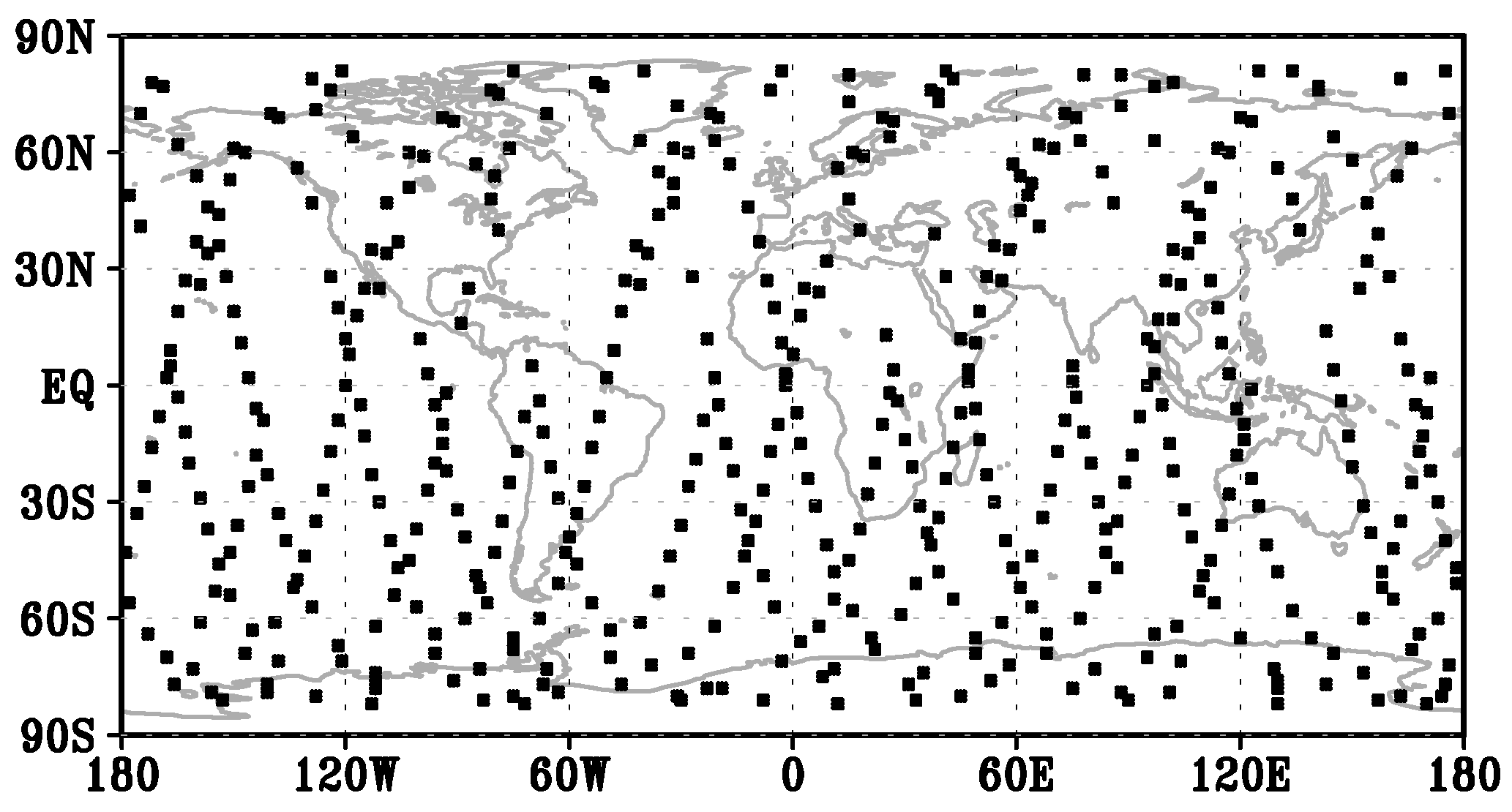
2. Data and Method
3. Climatology of the SWIs in the Stratosphere
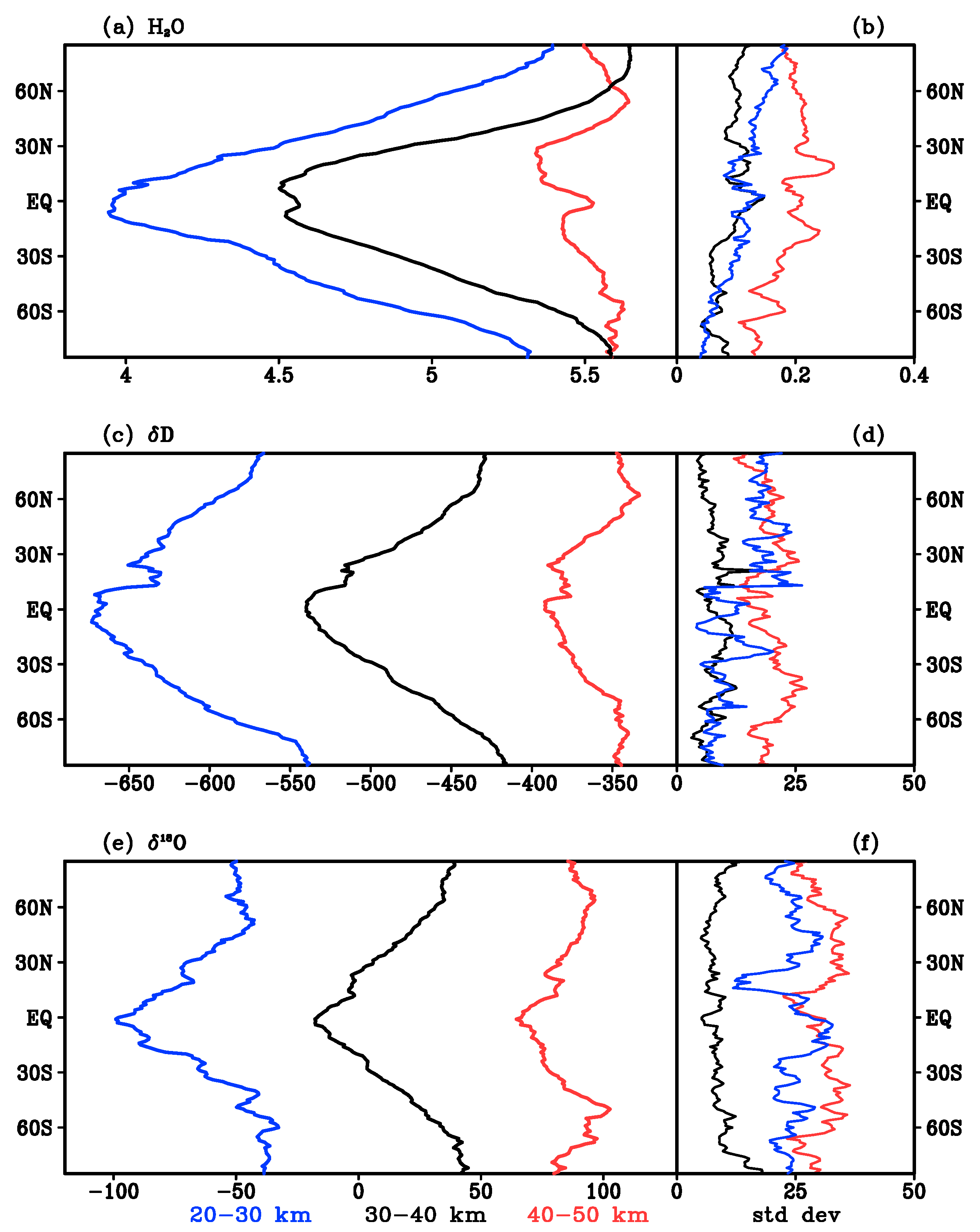
3.1. Global Mean Vertical Profiles
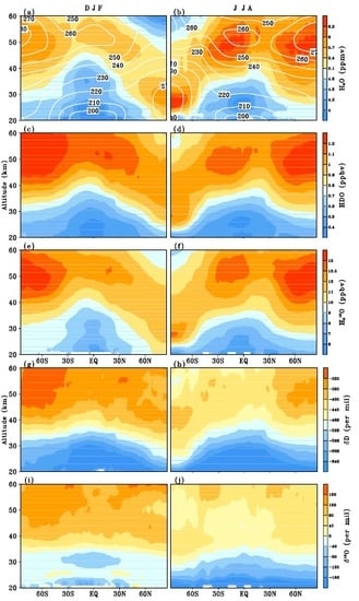
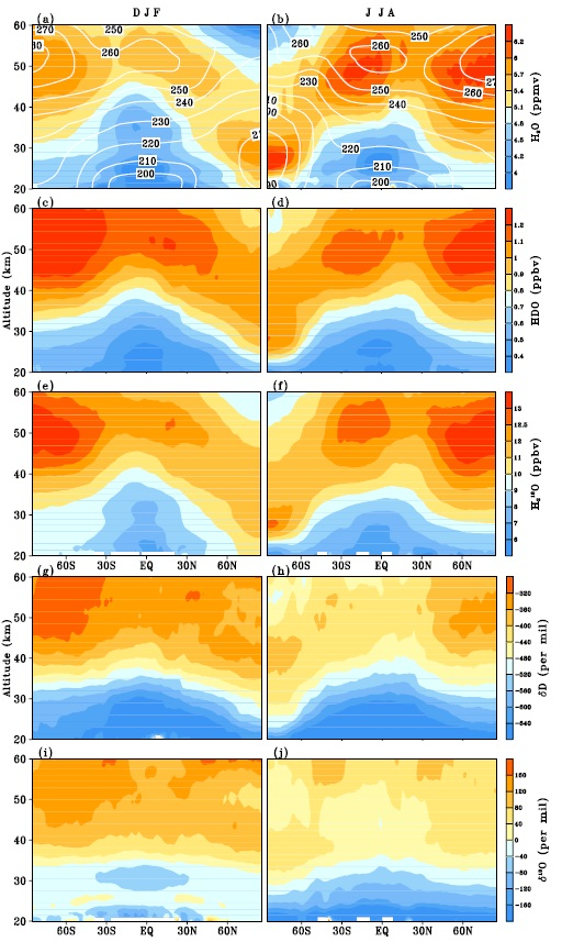
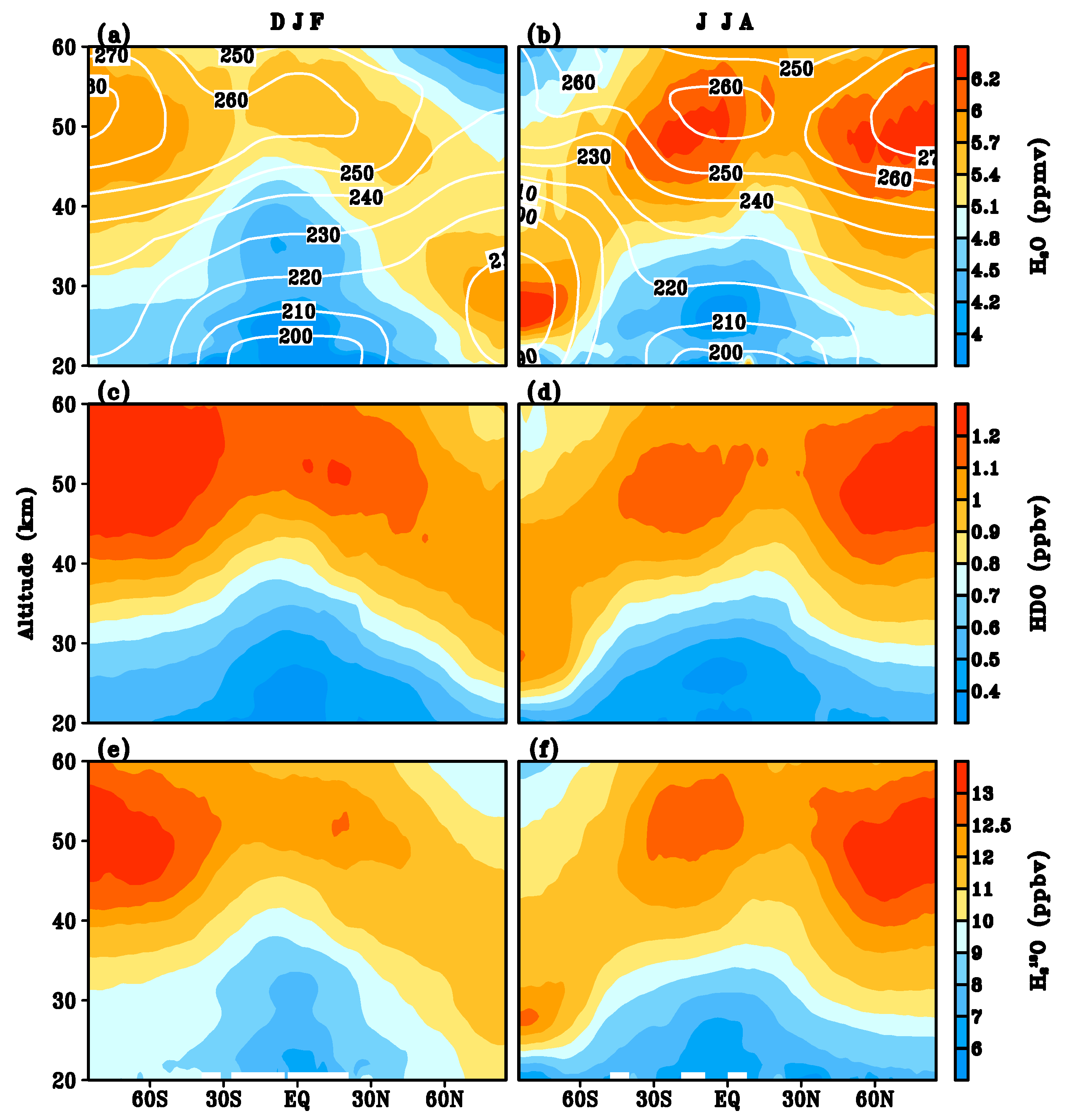
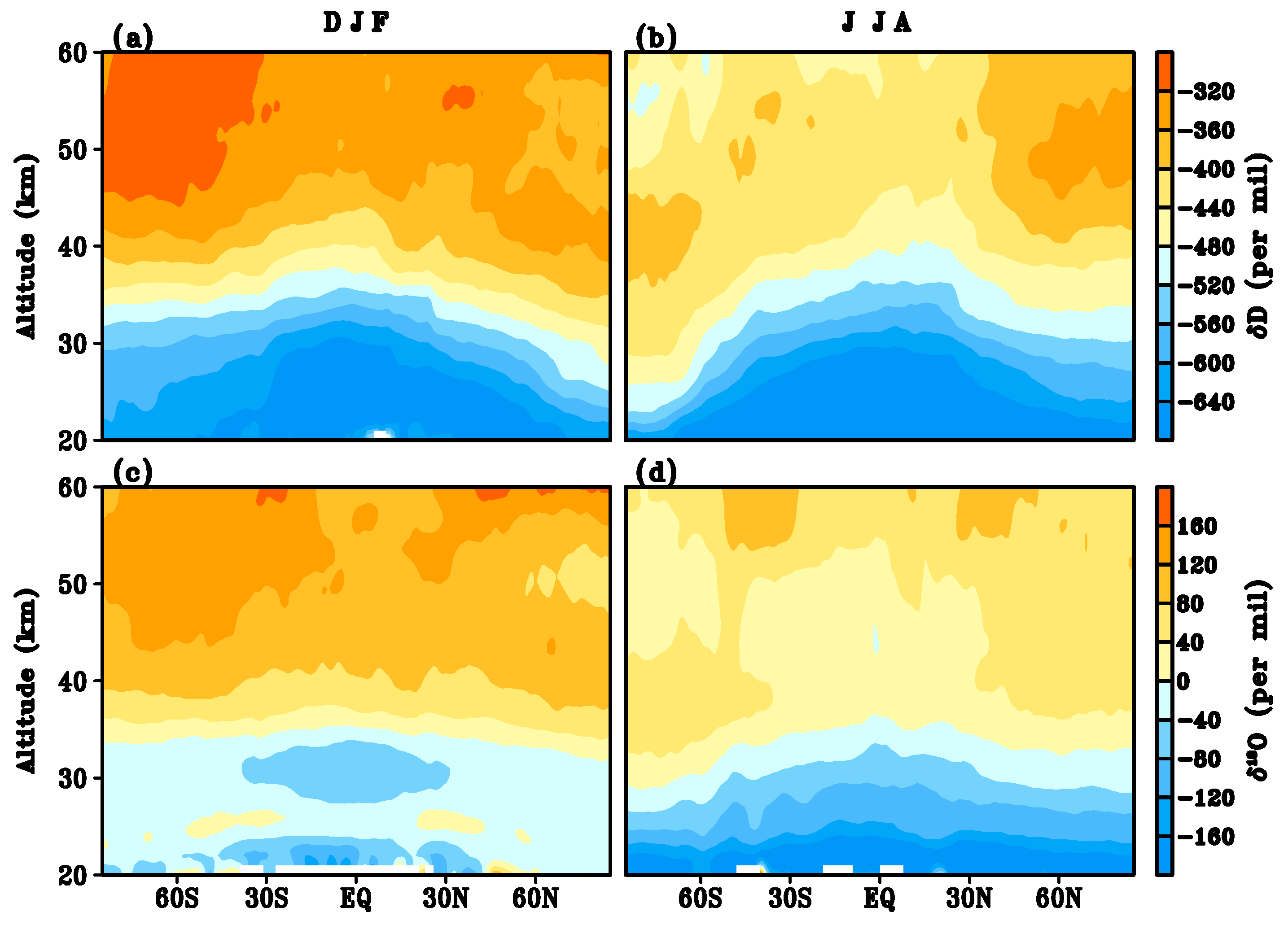
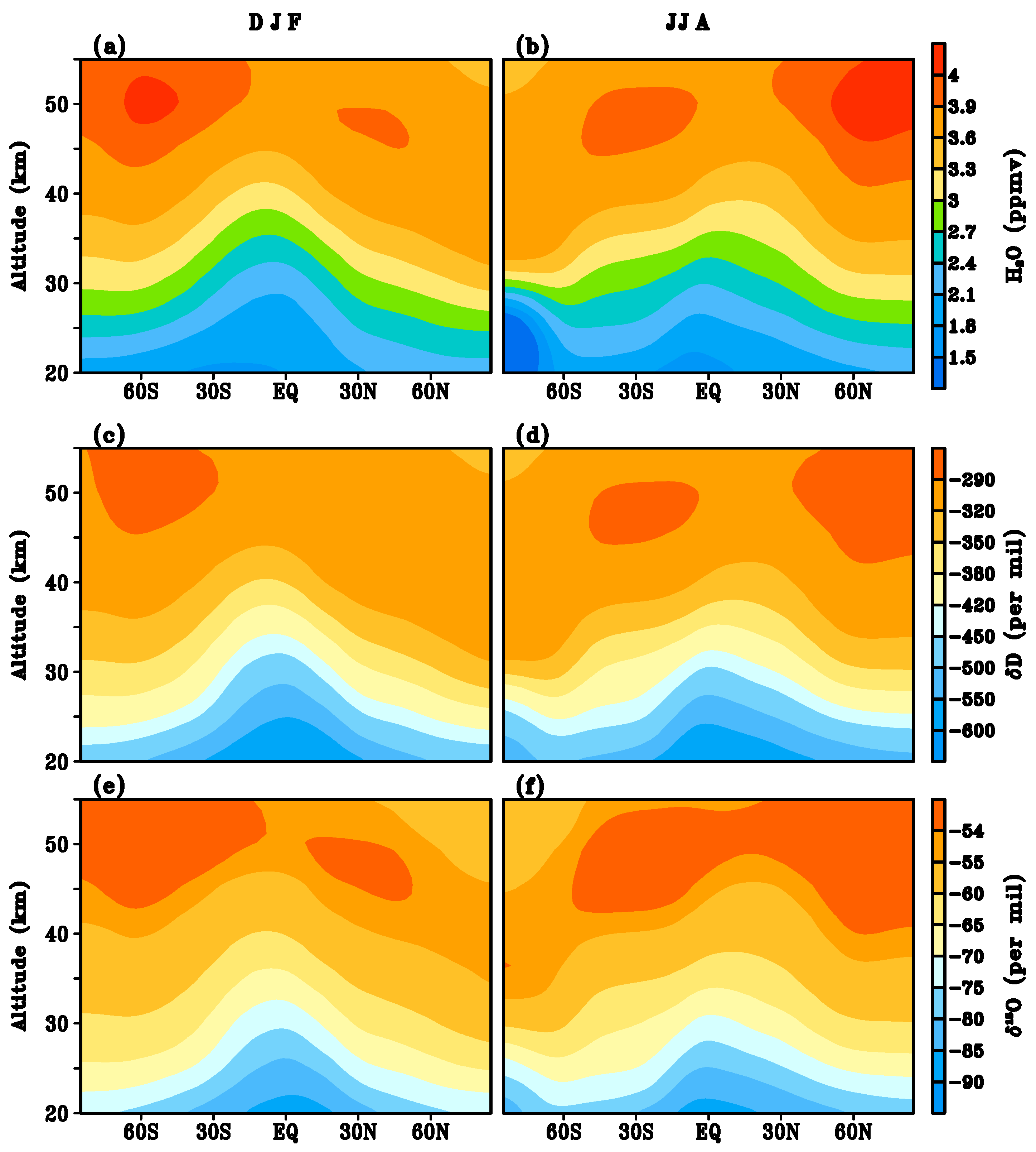
3.2. Zonal Mean Structure in the Lower and Upper Stratosphere
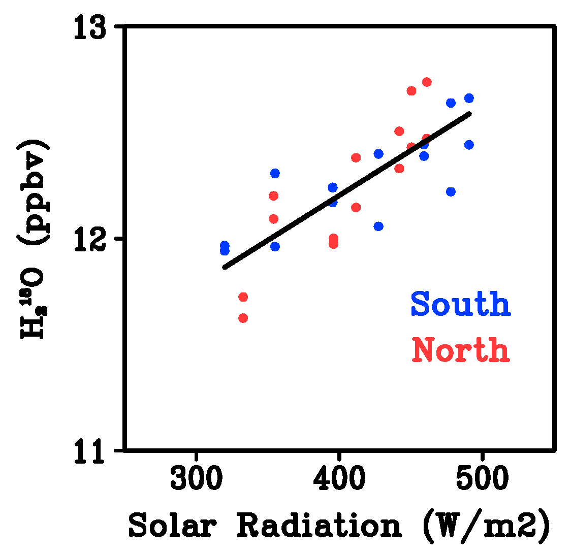
3.3. Seasonal Cycle and Related Processes
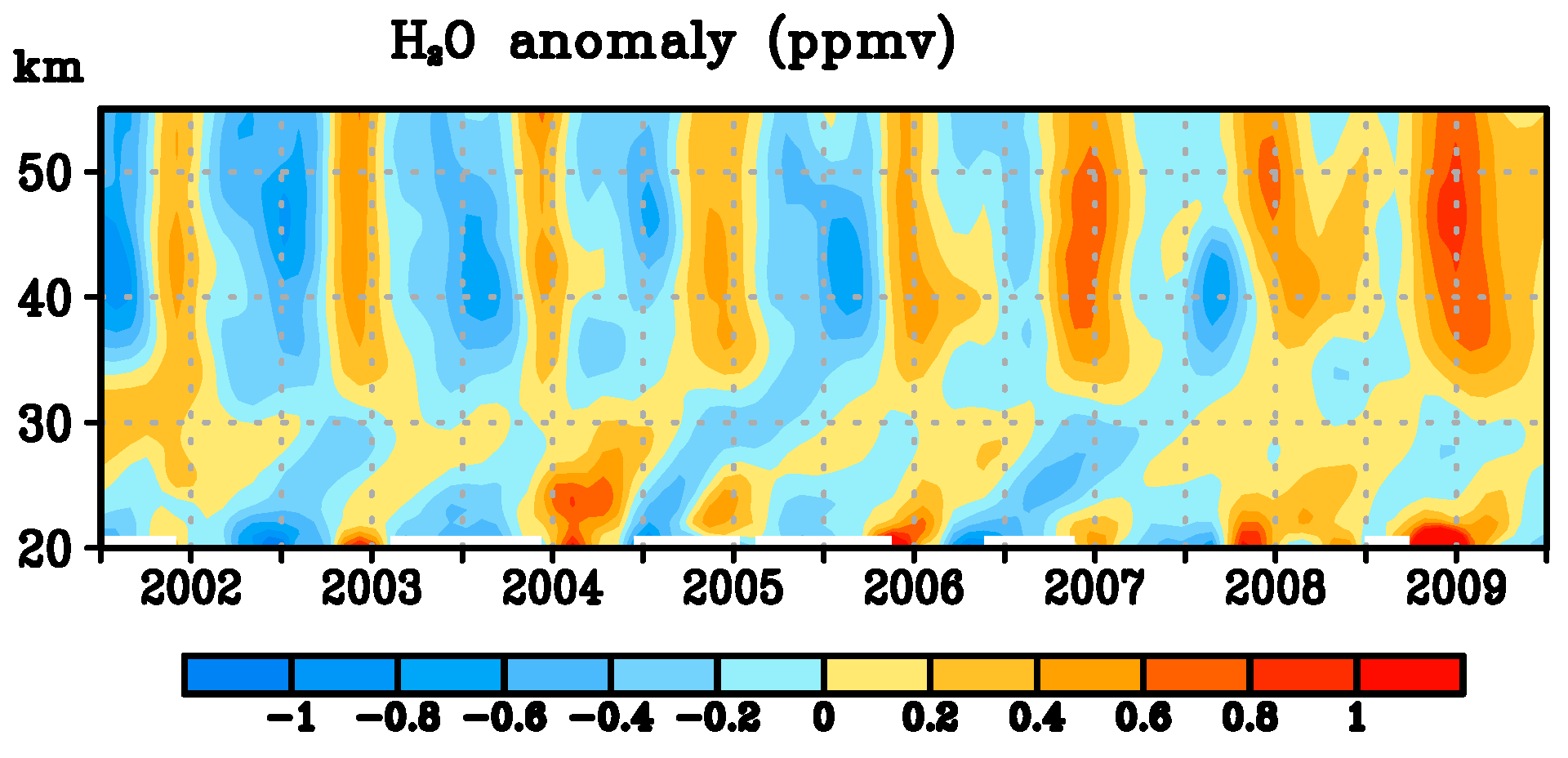
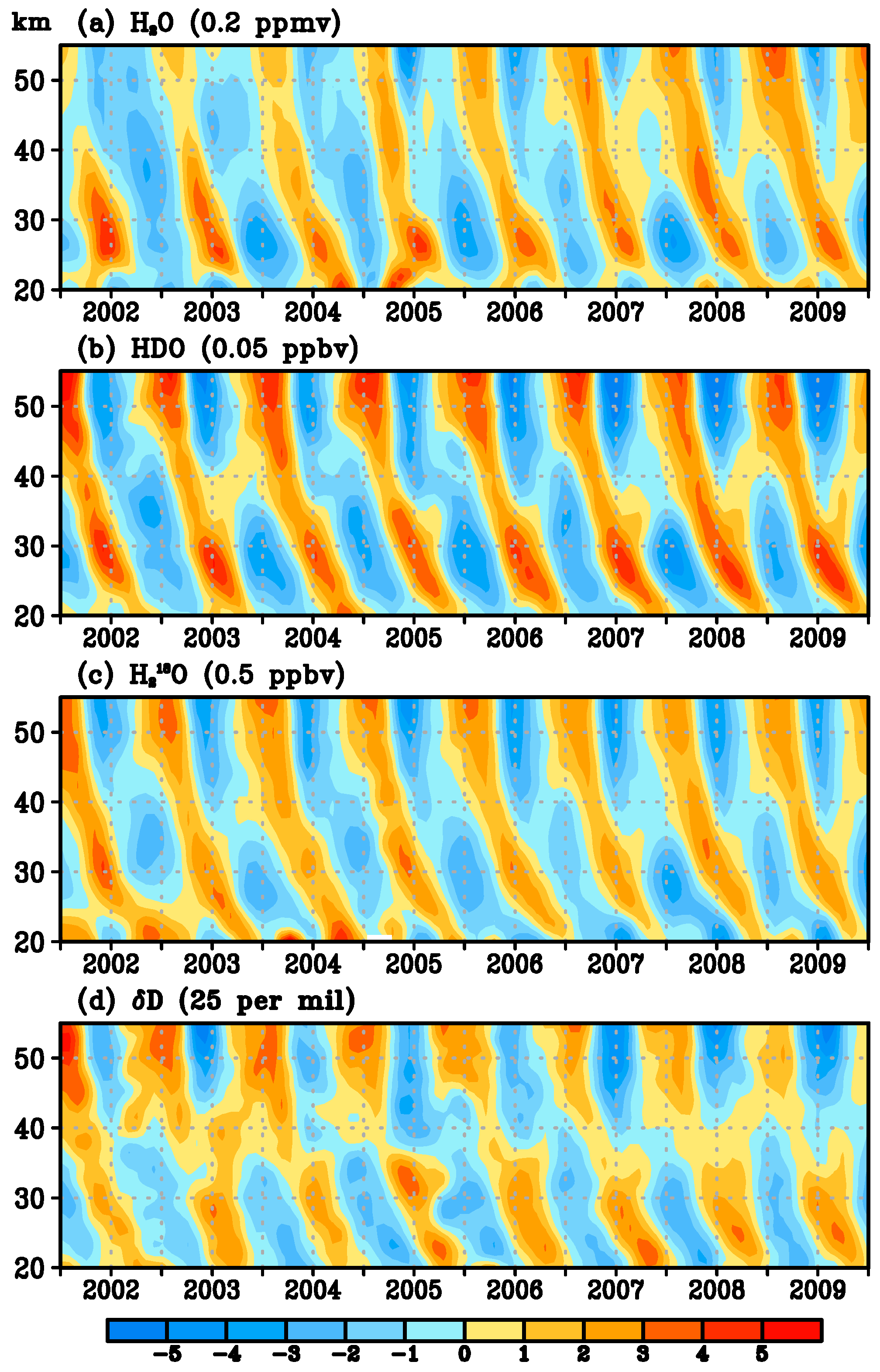
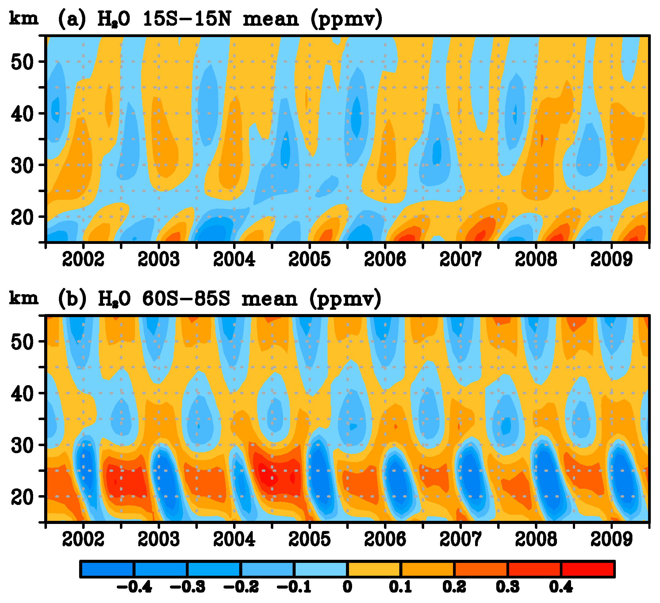
3.4. Vertical Propagation of Seasonal Signal
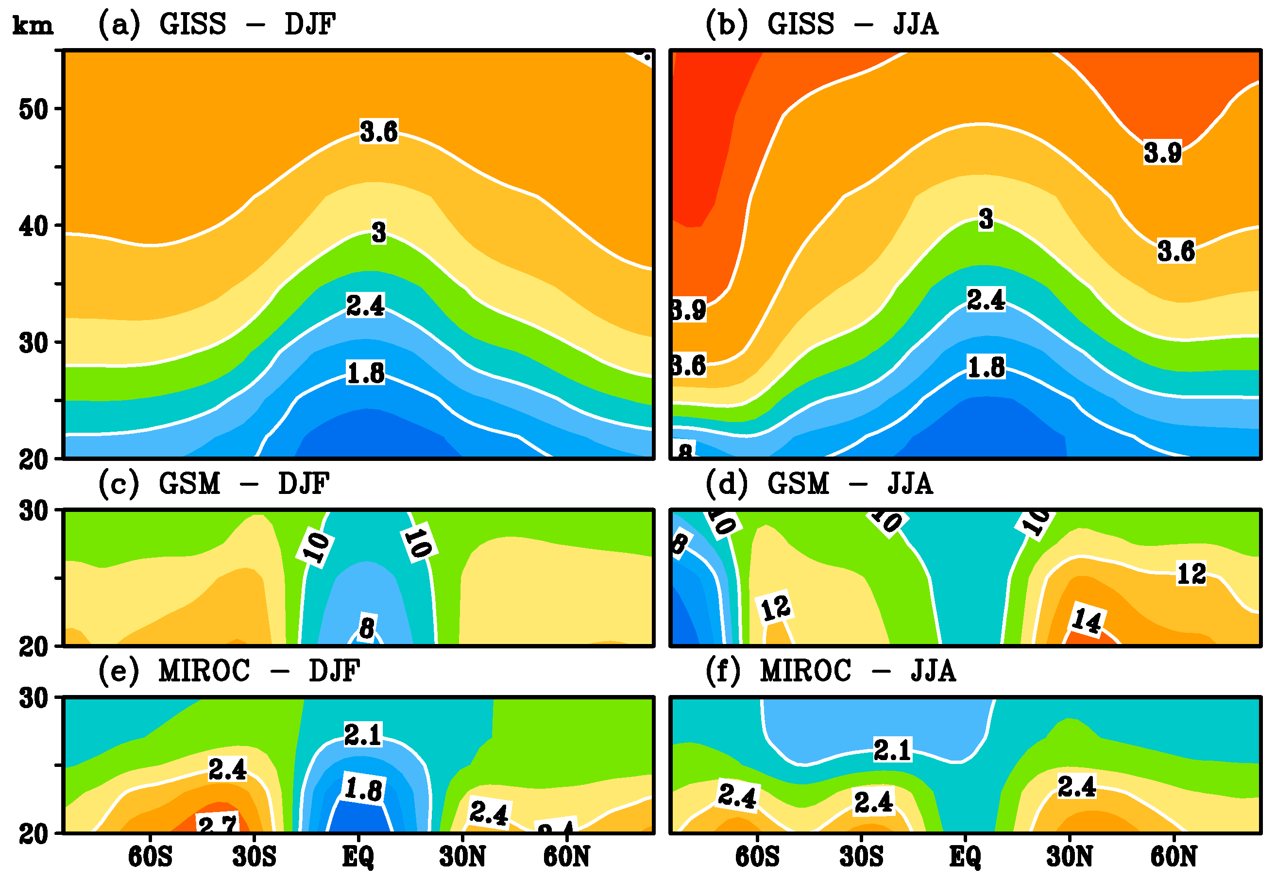
4. Comparison with SWI-Enabled GCM Simulation
5. Discussion
6. Conclusions
Acknowledgments
Author Contributions
Conflicts of Interest
References
- Solomon, S.; Rosenlof, K.H.; Portmann, R.W.; Daniel, J.S.; Davis, S.M.; Sanford, T.J.; Plattner, J.K. Contributions of stratospheric water vapor to decadal changes in the rate of global warming. Science 2010, 327, 1219–1223. [Google Scholar] [CrossRef] [PubMed]
- Dessler, A.; Schoeberl, M.R.; Wang, T.; Davis, S.M.; Rosenlof, K.H. Stratospheric water vapor feedback. Proc. Natl. Acad. Sci. USA 2013, 110, 18087–18091. [Google Scholar] [CrossRef] [PubMed]
- Johnson, D.G.; Jucks, K.W.; Traub, W.A.; Chance, K.V. Isotopic composition of stratospheric water vapor: Implications for transport. J. Geophys. Res. 2001, 106, 12219–12226. [Google Scholar] [CrossRef]
- Bechtel, C.; Zahn, A. The isotope composition of water vapour: A powerful tool to study transport and chemistry of middle atmospheric water vapour. Atmos. Chem. Phys. Discuss. 2003, 3, 3991–4036. [Google Scholar] [CrossRef]
- Brewer, A.W. Evidence for a world circulation provided by the measurements of helium and water vapour distribution in the stratosphere. Q. J. R. Meteorol. Soc. 1949, 75, 351–363. [Google Scholar] [CrossRef]
- Dobson, G.M.B. Origin and distribution of the polyatomic molecules in the atmosphere. Proc. R. Soc. Lond. Ser. A Math. Phys. Sci. 1956, 236, 187–193. [Google Scholar] [CrossRef]
- Gettelman, A.; Kinnison, D.E.; Dunkerton, T.J.; Brasseur, G.P. Impact of monsoon circulations on the upper troposphere and lower stratosphere. J. Geophys. Res. 2004, 109. [Google Scholar] [CrossRef]
- Khaykin, S.; Pommereau, J.P.; Korshunov, L.; Yushkov, V.; Nielsen, J.; Larsen, N.; Christensen, T.; Garnier, A.; Lukyanov, A.; Williams, E. Hydration of the lower stratosphere by ice crystal geysers over land convective systems. Atmos. Chem. Phys. 2009, 9, 2275–2287. [Google Scholar] [CrossRef]
- Zahn, A. Constraints on 2-way transport across the Arctic tropopause based on O3, stratospheric tracer (SF6) ages, and water vapor isotope (D, T) tracers. J. Atmos. Chem. 2001, 39, 303–325. [Google Scholar] [CrossRef]
- Texier, H.L.; Solomon, S.; Garcia, R.R. The role of molecular hydrogen and methane oxidation in the water vapour budget of the stratosphere. Q. J. R. Meteorol. Soc. 1988, 114, 281–295. [Google Scholar] [CrossRef]
- Ravishankara, A.R. Kinetics of radical reactions in the atmospheric oxidation of CH4. Annu. Rev. Phys. Chem. 1988, 39, 367–394. [Google Scholar] [CrossRef]
- Röckmann, T.; Rhee, T.S.; Engel, A. Heavy hydrogen in the stratosphere. Atmos. Chem. Phys. 2003, 3, 2015–2023. [Google Scholar] [CrossRef]
- Lyons, J.R. Transfer of mass-independent fractionation in ozone to other oxygen-containing radicals in the atmosphere. Geophys. Res. Lett. 2001, 28, 3231–3234. [Google Scholar] [CrossRef]
- Rinsland, C.P.; Gunson, M.R.; Foster, J.C.; Toth, R.A.; Farmer, C.B.; Zander, R. Stratospheric profiles of heavy water vapor isotopes and CH3D from analysis of the ATMOS Spacelab 3 infrared solar spectra. J. Geophys. Res. 1991, 96, 1057–1068. [Google Scholar] [CrossRef]
- Worden, J. Tropospheric Emission Spectrometer observations of the tropospheric HDO/H2O ratio: Estimation approach and characterization. J. Geophys. Res. 2006, 111, D16309. [Google Scholar] [CrossRef]
- Steinwagner, J.; Milz, M.; Clarmann, T.V.; Glatthor, N.; Grabowski, U.; Höpfner, M.; Stiller, G.; Röckmann, T. HDO measurements with MIPAS. Atmos. Chem. Phys. 2007, 7, 2601–2615. [Google Scholar] [CrossRef]
- Payne, V.H.; Noone, D.; Dudhia, A.; Piccolo, C.; Graingerb, R.G. Global satellite measurements of HDO and implications for understanding the transport of water vapour into the stratosphere. Q. J. R. Meteorol. Soc. 2007, 133, 1459–1471. [Google Scholar] [CrossRef]
- Steinwagner, J.; Fueglistaler, S.; Stiller, G.; Clarmann, T.V.; Kiefer, M.; Borsboom, P.P.; Delden, A.V.; Röckmann, T. Tropical dehydration processes constrained by the seasonality of stratospheric deuterated water. Nat. Geosci. 2010, 3, 262–266. [Google Scholar] [CrossRef]
- Randel, W.J.; Moyer, E.; Park, M.; Jensen, E.; Bernath, P.; Walker, K.; Boone, C. Global variations of HDO and HDO/H2O ratios in the upper troposphere and lower stratosphere derived from ACE-FTS satellite measurements. J. Geophys. Res. 2012, 117, D06303. [Google Scholar] [CrossRef]
- Zelinger, Z.; Barret, B.; Kubát, P.; Ricaud, P.; Attie, J.L.; Flochmoën, L.E.; Urban, J.; Murtagh, D.; Střižík, M. Observation of HD18O, CH3OH and vibrationally-excited N2O from Odin/SMR measurements. Mol. Phys. 2006, 104, 2815–2820. [Google Scholar] [CrossRef]
- Nassar, R.; Bernath, P.F.; Boone, C.D.; Gettelman, A.; McLeod, S.D.; Rinsland, C.P. Variability in HDO/H2O abundance ratios in the tropical tropopause layer. J. Geophys. Res. 2007, 112, D21305. [Google Scholar] [CrossRef]
- Schmidt, G.A.; Hoffmann, G.; Shindell, D.T.; Hu, Y. Modeling atmospheric stable water isotopes and the potential for constraining cloud processes and stratosphere—Troposphere water exchange. J. Geophys. Res. 2005, 110, D21314. [Google Scholar] [CrossRef]
- Noone, D. Evaluation of hydrological cycles and processes with water isotopes: Report to GEWEX-GHP from the Stable Water-isotope Intercomparison Group (SWING). In Proceedings of the Pan-GEWEX Meeting, Frascati, Italy, 9–13 October 2006. [Google Scholar]
- Risi, C.; Noone, D.; Worden, J.; Frankenberg, C.; Stiller, G.; Kiefer, M.; Funke, B.; Walker, K.; Bernath, P.; Schneider, M. Process-evaluation of tropospheric humidity simulated by general circulation models using water vapor isotopologues: 1. Comparison between models and observations. J. Geophys. Res. 2012, 117, D05303. [Google Scholar] [CrossRef]
- Risi, C.; Noone, D.; Worden, J.; Frankenberg, C.; Stiller, G.; Kiefer, M.; Funke, B.; Walker, K.; Bernath, P.; Schneider, M. Process-evaluation of tropospheric humidity simulated by general circulation models using water vapor isotopic observations: 2. Using isotopic diagnostics to understand the mid and upper tropospheric moist bias in the tropics and subtropics. J. Geophys. Res. Atmos. 2012, 117, 214–221. [Google Scholar] [CrossRef]
- Conroy, J.L.; Cobb, K.M.; Noone, D. Comparison of precipitation isotope variability across the tropical Pacific in observations and SWING2 model simulations. J. Geophys. Res. Atmos. 2013, 118, 5867–5892. [Google Scholar] [CrossRef]
- Hourdin, F.; Musat, I.; Bony, S.; Braconnot, P.; Codron, F.; Dufresne, J.L.; Fairhead, L.; Filiberti, M.A.; Friedlingstein, P.; Grandpeix, J.Y.; et al. The LMDZ general circulation model: Climate performance and sensitivity to parametrized physics with emphasis on tropical convection. Clim. Dyn. 2006, 27, 787–813. [Google Scholar] [CrossRef]
- Murtagh, D.; Frisk, U.; Merino, F.; Ridal, M.; Jonsson, A.; Stegman, J.; Witt, G.; Eriksson, P.; Jiménez, C.; Megie, G. An overview of the Odin atmospheric mission. Can. J. Phys. 2002, 80, 309–319. [Google Scholar] [CrossRef]
- Urban, J.; Lautié, N.; Murtagh, D.; Eriksson, P.; Kasai, Y.; Lossow, S.; Dupuy, E.; De La Noë, J.; Frisk, U.; Olberg, M.; et al. Global observations of middle atmospheric water vapour by the Odin satellite: An overview. Planet. Space Sci. 2007, 55, 1093–1102. [Google Scholar] [CrossRef]
- Urban, J.; Lautié, N.; Flochmoën, E.L.; Jiménez, C.; Eriksson, P.; Noë, J.L.; Dupuy, E.; Ekström, M.; Amraoui, L.E.; Frisk, U. Odin/SMR limb observations of stratospheric trace gases: Level 2 processing of ClO, N2O, HNO3, and O3. J. Geophys. Res. 2005, 110, D14307. [Google Scholar] [CrossRef]
- Jones, A.; Walker, K.A.; Jin, J.J.; Taylor, J.R.; Boone, C.D.; Bernath, P.F.; Brohede, S.; Manney, G.L.; McLeod, S.; Hughes, R.; et al. Technical Note: A trace gas climatology derived from the Atmospheric Chemistry Experiment Fourier Transform Spectrometer (ACE-FTS) data set. Atmos. Chem. Phys. 2012, 12, 5207–5220. [Google Scholar] [CrossRef]
- Rienecker, M.M.; Suarez, M.J.; Gelaro, R.; Todling, R.; Bacmeister, J.; Liu, E.; Bosilovich, M.G.; Schubert, S.D.; Takacs, L.; Kim, G.K. MERRA: NASA’s modern-era retrospective analysis for research and applications. J. Clim. 2011, 24, 3624–3648. [Google Scholar] [CrossRef]
- Coddington, O.; Lean, J.L.; Pilewskie, P.; Snow, M.; Lindholm, D. A solar irradiance climate data record. Bull. Am. Meteorol. Soc. 2015, 97, 1265–1282. [Google Scholar] [CrossRef]
- International Atomic Energy Agency (IAEA). Reference Sheet for VSMOW2 and SLAP2 International Measurement Standards; International Atomic Energy Agency: Vienna, Austria, 2009; p. 5. [Google Scholar]
- Lossow, S.; Steinwagner, J.; Urban, J.; Dupuy, E.; Boone, C.D.; Kellmann, S.; Linden, A.; Kiefer, M.; Grabowski, U.; Glatthor, N.; et al. Comparison of HDO measurements from Envisat/MIPAS with observations by Odin/SMR and SCISAT/ACE-FTS. Atmos. Meas. Tech. 2011, 4, 1855–1874. [Google Scholar] [CrossRef]
- Hurst, D.F.; Oltmans, S.J.; Vömel, H.; Rosenlof, K.H.; Davis, S.M.; Ray, E.A.; Hall, E.G.; Jordan, A.F. Stratospheric water vapor trends over Boulder, Colorado: Analysis of the 30 year Boulder record. J. Geophys. Res. 2011, 116, D02306. [Google Scholar] [CrossRef]
- Dessler, A.; Sherwood, S. A model of HDO in the tropical tropopause layer. Atmos. Chem. Phys. 2003, 3, 2173–2181. [Google Scholar] [CrossRef]
- Dessler, A.; Sherwood, S. Effect of convection on the summertime extratropical lower stratosphere. J. Geophys. Res. 2004, 109, D23301. [Google Scholar] [CrossRef]
- Moyer, E.J.; Irion, F.W.; Yung, Y.L.; Gunson, M.R. ATMOS stratospheric deuterated water and implications for troposphere-stratosphere transport. Geophys. Res. Lett. 1996, 23, 2385–2388. [Google Scholar] [CrossRef]
- Stiller, G.P.; Clarmann, T.V.; Haenel, F.; Funke, B.; Glatthor, N.; Grabowski, U.; Kellmann, S.; Kiefer, M.; Linden, A.; Lossow, S. Observed temporal evolution of global mean age of stratospheric air for the 2002 to 2010 period. Atmos. Chem. Phys. 2012, 12, 3311–3331. [Google Scholar] [CrossRef]
- Holton, J.R.; Haynes, P.H.; Mcintyre, M.E.; Douglass, A.R.; Rood, R.B.; Pfister, L. Stratosphere-troposphere exchange. Rev. Geophys. 1995, 33, 403–439. [Google Scholar] [CrossRef]
- Dunkerton, T. On the mean meridional mass motions of the stratosphere and mesosphere. J. Atmos. Sci. 1978, 35, 2325–2333. [Google Scholar] [CrossRef]
- Randel, W.J.; Wu, F.; Russell, J.M., III; Roche, A.; Waters, J.W. Seasonal cycles and QBO variations in stratospheric CH4 and H2O observed in UARS HALOE data. J. Atmos. Sci. 1998, 55, 163–185. [Google Scholar] [CrossRef]
- Mote, P.W.; Rosenlof, K.H.; McIntyre, M.E.; Carr, E.S.; Gille, J.C.; Holton, J.R.; Kinnersley, J.S.; Pumphrey, H.C.; Russell, J.M.; Waters, J.W. An atmospheric tape recorder: The imprint of tropical tropopause temperatures on stratospheric water vapor. J. Geophys. Res. 1996, 101, 3989–4006. [Google Scholar] [CrossRef]
- Eichinger, R.; Jöckel, P.; Brinkop, S.; Werner, M.; Lossow, S. Simulation of the isotopic composition of stratospheric water vapour–Part 1: Description and evaluation of the EMAC model. Atmos. Chem. Phys. 2015, 15, 5537–5555. [Google Scholar] [CrossRef]
- Sturm, C.; Zhang, Q.; Noone, D. An introduction to stable water isotopes in climate models: Benefits of forward proxy modelling for paleoclimatology. Clim. Past 2010, 6, 115–129. [Google Scholar] [CrossRef]
- Risi, C.; Bony, S.; Vimeux, F.; Jouzel, J. Water-stable isotopes in the LMDZ4 general circulation model: Model evaluation for present-day and past climates and applications to climatic interpretations of tropical isotopic records. J. Geophys. Res. 2010, 115, D12118. [Google Scholar] [CrossRef]
- Marti, O.; Braconnot, P.; Bellier, J.; Benshile, R.; Bony, S.; Brockmann, P.; Cadulle, P.; Caubel, A.; Denvil, S.; Dufresne, J.L.; et al. The New IPSL Climate System Model: IPSL-CM4; Institut Pierre Simon Laplace: Paris, France, 2005; 86p. [Google Scholar]
- Emanuel, K.A.; Živković-Rothman, M. Development and evaluation of a convection scheme for use in climate models. J. Atmos. Sci. 1999, 56, 1766–1782. [Google Scholar] [CrossRef]
- Bony, S.; Emanuel, K.A. A parameterization of the cloudiness associated with cumulus convection; evaluation using TOGA COARE data. J. Atmos. Sci. 2001, 58, 3158–3183. [Google Scholar] [CrossRef]
- Klinker, E.; Rabier, F.; Kelly, G.; Mahfouf, J.F. The ecmwf operational implementation of four-dimensional variational assimilation. III: Experimental results and diagnostics with operational configuration. Q. J. R. Meteorol. Soc. 2000, 126, 1191–1215. [Google Scholar] [CrossRef]
- Van, L.B. Towards the ultimate conservative difference scheme. V. A second-order sequel to Godunov’s method. J. Comput. Phys. 1979, 32, 101–136. [Google Scholar]
- Brasseur, G.; Solomon, S. Aeronomy of the Middle Atmosphere; D. Reidel Publishing Co.: Dordrecht, The Netherlands, 1984. [Google Scholar]
- Lott, F.; Fairhead, L.; Hourdin, F.; Levan, P. The stratospheric version of LMDz: Dynamical Climatologies, Arctic Oscillation, and Impact on the Surface Climate. Clim. Dyn. 2005, 25, 851–868. [Google Scholar] [CrossRef]
- Schmidt, G.; LeGrande, A.; Hoffmann, G. Water isotope expressions of intrinsic and forced variability in a coupled ocean-atmosphere model. J. Geophys. Res. 2007, 112, D10103. [Google Scholar] [CrossRef]
- Yoshimura, K.; Kanamitsu, M.; Noone, D.; Oki, T. Historical isotope simulation using Reanalysis atmospheric data. J. Geophys. Res. 2008, 113, D19108. [Google Scholar] [CrossRef]
- Kurita, K.; Noone, D.; Risi, C.; Schmidt, G.A.; Yamada, H.; Yoneyama, K. Intraseasonal isotopic variation associated with the Madden-Julian Oscillation. J. Geophys. Res. 2011, 116, D24101. [Google Scholar] [CrossRef]
- Gates, W.L. AMIP: The atmospheric model intercomparison project. Bull. Am. Meteorol. Soc. 1992, 73, 1962–1970. [Google Scholar] [CrossRef]
- Godunov, S.K. A difference method for numerical calculation of discontinuous solutions of the equations of hydrodynamics. Mat. Sb. 1959, 89, 271–306. [Google Scholar]
- Craig, H. Isotopic variations in meteoric waters. Science 1961, 133, 1702–1703. [Google Scholar] [CrossRef] [PubMed]
- Dansgaard, W. Stable isotopes in precipitation. Tellus 1964, 16, 436–468. [Google Scholar] [CrossRef]


© 2018 by the authors. Licensee MDPI, Basel, Switzerland. This article is an open access article distributed under the terms and conditions of the Creative Commons Attribution (CC BY) license (http://creativecommons.org/licenses/by/4.0/).
Share and Cite
Wang, T.; Zhang, Q.; Lossow, S.; Chafik, L.; Risi, C.; Murtagh, D.; Hannachi, A. Stable Water Isotopologues in the Stratosphere Retrieved from Odin/SMR Measurements. Remote Sens. 2018, 10, 166. https://doi.org/10.3390/rs10020166
Wang T, Zhang Q, Lossow S, Chafik L, Risi C, Murtagh D, Hannachi A. Stable Water Isotopologues in the Stratosphere Retrieved from Odin/SMR Measurements. Remote Sensing. 2018; 10(2):166. https://doi.org/10.3390/rs10020166
Chicago/Turabian StyleWang, Tongmei, Qiong Zhang, Stefan Lossow, Léon Chafik, Camille Risi, Donal Murtagh, and Abdel Hannachi. 2018. "Stable Water Isotopologues in the Stratosphere Retrieved from Odin/SMR Measurements" Remote Sensing 10, no. 2: 166. https://doi.org/10.3390/rs10020166
APA StyleWang, T., Zhang, Q., Lossow, S., Chafik, L., Risi, C., Murtagh, D., & Hannachi, A. (2018). Stable Water Isotopologues in the Stratosphere Retrieved from Odin/SMR Measurements. Remote Sensing, 10(2), 166. https://doi.org/10.3390/rs10020166