Retrieval Accuracy of HCHO Vertical Column Density from Ground-Based Direct-Sun Measurement and First HCHO Column Measurement Using Pandora

Abstract

In the present study, we investigate the effects of signal to noise (SNR), slit function (FWHM), and aerosol optical depth (AOD) on the accuracy of formaldehyde (HCHO) vertical column density (HCHO_VCD) using the ground-based direct-sun synthetic radiance based on differential optical absorption spectroscopy (DOAS). We found that the effect of SNR on HCHO retrieval accuracy is larger than those of FWHM and AOD. When SNR = 650 (1300), FWHM = 0.6, and AOD = 0.2, the absolute percentage difference (APD) between the true HCHO_VCD values and those retrieved ranges from 54 (30%) to 5% (1%) for the HCHO_VCD of 5.0 × 10¹⁵ and 1.1 × 10¹⁷ molecules cm⁻², respectively. Interestingly, the maximum AOD effect on the HCHO accuracy was found for the HCHO_VCD of 3.0 × 10¹⁶ molecules cm⁻². In addition, we carried out the first ground-based direct-sun measurements in the ultraviolet (UV) wavelength range to retrieve the HCHO_VCD using Pandora in Seoul. The HCHO_VCD was low at 12:00 p.m. local time (LT) in all seasons, whereas it was high in the morning (10:00 a.m. LT) and late afternoon (4:00 p.m. LT), except in winter. The maximum HCHO_VCD values were 2.68 × 10¹⁶, 3.19 × 10¹⁶, 2.00 × 10¹⁶, and 1.63 × 10¹⁶ molecules cm⁻² at 10:00 a.m. LT in spring, 10:00 a.m. LT in summer, 1:00 p.m. LT in autumn, and 9:00 a.m. LT in winter, respectively. The minimum values of Pandora HCHO_VCD were 1.63 × 10¹⁶, 2.23 × 10¹⁶, 1.26 × 10¹⁶, and 0.82 × 10¹⁶ molecules cm⁻² at around 1:45 p.m. LT in spring, summer, autumn, and winter, respectively. This seasonal pattern of high values in summer and low values in winter implies that photo-oxidation plays an important role in HCHO production. The correlation coefficient (R) between the monthly HCHO_VCD values from Pandora and those from the Ozone Monitoring Instrument (OMI) is 0.61, and the slope is 1.25.

1. Introduction

Despite its relatively short atmospheric lifetime [1,2,3], which is less than five hours near the surface [4], formaldehyde (HCHO) is one of the most abundant carbonyl compounds in the atmosphere. HCHO in the atmosphere has a surface mixing ratio of several tens of ppbv in a polluted atmosphere [5,6,7,8]; in an uncontaminated atmosphere, it has a background concentration of several tens of pptv [9,10,11,12].

Atmospheric HCHO levels have been measured for more than 15 years using satellite sensors from the Global Ozone Monitoring Experiment (GOME) onboard the European Remote Sensing-2 satellite (ERS-2) launched in April 1995, the SCanning Imaging Absorption SpectroMeter for Atmospheric CHartographY (SCIAMACHY) onboard the European Environment Satellite (ENVISAT) launched in March 2002, the Atmospheric Chemistry Experiment-Fourier Transform Spectrometer (ACE-FTS) onboard the Science Satellite (SCISAT-1) launched in August 2003, the Ozone Monitoring Instrument (OMI) on the Aura satellite launched in June 2004, GOME-2 onboard the Meteorological Operational satellites launched in January 2007 (MetOp-A) and September 2012 (MetOp-B), and the Ozone Mapping and Profiler Suite (OMPS) on the Suomi National Polar-orbiting Partnership (Suomi NPP) satellite launched in October 2011. Each of these satellites uses a different fitting window to retrieve the HCHO data. The GOME, SCIAMACHY, OMI, GOME-2, and OMPS sensors have fitting windows of 337.0–359.0, 334.0–348.0, 328.5–356.5, 328.5–346, and 328.5–356.5 nm, respectively.

Chance et al. [13] retrieved HCHO data for North America from GOME measurements. De Smedt et al. [14] calculated the global tropospheric vertical column density (VCD) of HCHO (HCHO_VCD) based on the GOME and SCIAMACHY measurements and reported the temporal trend in HCHO between 1997 and 2009. To investigate the spatiotemporal characteristics of the HCHO column between 2004 and 2014, De Smedt et al. [15] used data from SCIAMACHY, GOME-2, and OMI to develop a new version (v14) of the BIRA-IASB algorithm for HCHO retrieval.

A number of ground-based HCHO retrieval studies have also been conducted to validate the satellite-based HCHO observations using various ground-based remote sensing techniques. In particular, Multi-AXis Differential Optical Absorption Spectroscopy (MAX-DOAS), which is highly sensitive to trace gases in the planetary boundary layer (PBL) and uses scattered sunlight as a light source to retrieve the column density of HCHO in the atmosphere, has been used successfully in several studies. Among these MAX-DOAS studies of HCHO, Li et al. [16] retrieved the vertical HCHO distribution using a fitting window of 335.0–358.0 nm based on MAX-DOAS data from Shanghai, and reported the summertime diurnal characteristics of HCHO_VCD. Lee et al. [17] investigated diurnal variations in the vertical distribution of HCHO using a fitting window of 335.0–357.0 nm based on MAX-DOAS data from Beijing in summer, and compared these retrieved HCHO data with OMI HCHO data. Franco et al. [18] retrieved the vertical HCHO distribution using a fitting window of 328.5–358.0 nm with MAX-DOAS data and Fourier Transform InfraRed (FTIR) measurements from Jungfraujoch in Switzerland, and investigated the sensitivity difference of the vertical HCHO distribution between the two ground-based instruments. Previous HCHO-related MAX-DOAS studies are summarized in

Table 1. Summary of previous studies using Multi-AXis Differential Optical Absorption Spectroscopy (MAX-DOAS) measurements.

Study	Location	Date or Campaign	Target Species	Instrument	Unit
Heckel et al. [19]	Po Valley, Northern Italy	Formaldehyde as a tracer of photo oxidation in the Troposphere (FORMAT; summer 2002)	HCHO	MAX-DOAS	Mixing ratio
Vigouroux et al. [20]	Réunion Island	2004–2005 (2004–2007)	HCHO	MAX-DOAS, (FTIR)	Column density, Mixing ratio
Irie et al. [21]	Cabauw, the Netherlands	The Cabauw Intercomparison Campaign of Nitrogen Dioxide measuring Instruments (CINDI; summer 2009)	HCHO NO2 CHOCHO H2O SO2 O3	MAX-DOAS	Mixing ratio
Peters et al. [22]	Western Pacific Ocean	TransBrom campaign (9–24 October 2009)	HCHO NO2	MAX-DOAS	Column density
Pinardi et al. [23]	Cabauw, the Netherlands	The Cabauw Intercomparison Campaign of Nitrogen Dioxide measuring Instruments (CINDI; summer 2009)	HCHO	MAX-DOAS	Column density
Li et al. [16]	Shanghai, China	April 2010–April 2011	HCHO NO2	MAX-DOAS	Mixing ratio
De Smedt et al. [15]	Europe, China, and Africa	2004–2014	HCHO	MAX-DOAS, FTIR	Column density, Vertical profile
Lee et al. [17]	Beijing, China	Campaign of Air Quality Research in Beijing 2006 (CAREBEIJING-2006; August–September 2006)	HCHO O4	MAX-DOAS	Column density, Vertical profile
Franco et al. [18]	Jungfraujoch and Monch on the northern edge of the Swiss Alps	July 2010–December 2012	HCHO	MAX-DOAS, FTIR	Column density, Vertical profile

.

Among the instruments that use direct ultraviolet (UV) and visible sunlight as a light source, MultiFunction Differential Optical Absorption Spectroscopy (MFDOAS) has been used to measure NO₂ VCD at the Goddard Space Flight Center [24]. The Pandora Spectrometer Instrument (PSI) has also been used to retrieve O₃ VCD in Boulder, USA, and to retrieve NO₂ VCD in Maryland, USA, and in Thessaloniki, Greece [24,25]. Fioletov et al. [26] retrieved SO₂ VCD data from Pandora measurements in the Canadian oil sands region. To date, no studies have measured the HCHO column using MFDOAS or Pandora.

To use a ground-based instrument as a tool to validate satellite products, the accuracy of the data obtained from the ground-based instrument must be quantified and understood. We understand some of the retrieval uncertainty associated with MAX-DOAS measurement since there have been many studies that reported the retrieval accuracy of MAX-DOAS [22,27,28]. However, although there are either no, or negligible, air mass factor (AMF) errors in ground-based direct-sun measurements, the light absorption path length of direct-sun measurements is generally shorter than that of scattered-sun light measurements made using MAX-DOAS in most regions, which implies that the retrieval sensitivity of direct-sun measurements with respect to trace gases in PBL such as HCHO is lower than that of MAX-DOAS. Unfortunately, there is no information available regarding the errors associated with the products retrieved from such ground-based direct-sun measurements using the DOAS technique.

Therefore, the aims of this study are as follows: (1) to quantify the effects of signal-to-noise ratios (SNR), slit function (FWHM), and aerosol optical depth (AOD) on the HCHO_VCD accuracy of DOAS HCHO retrieval at various HCHO levels obtained from ground-based direct-sun measurement; (2) to retrieve, for the first time, HCHO_VCD using Pandora data and compare this with the values retrieved from the OMI in Seoul, South Korea; (3) to analyze the seasonal and diurnal characteristics of the retrieved HCHO columns from Seoul.

2. Methods

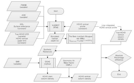
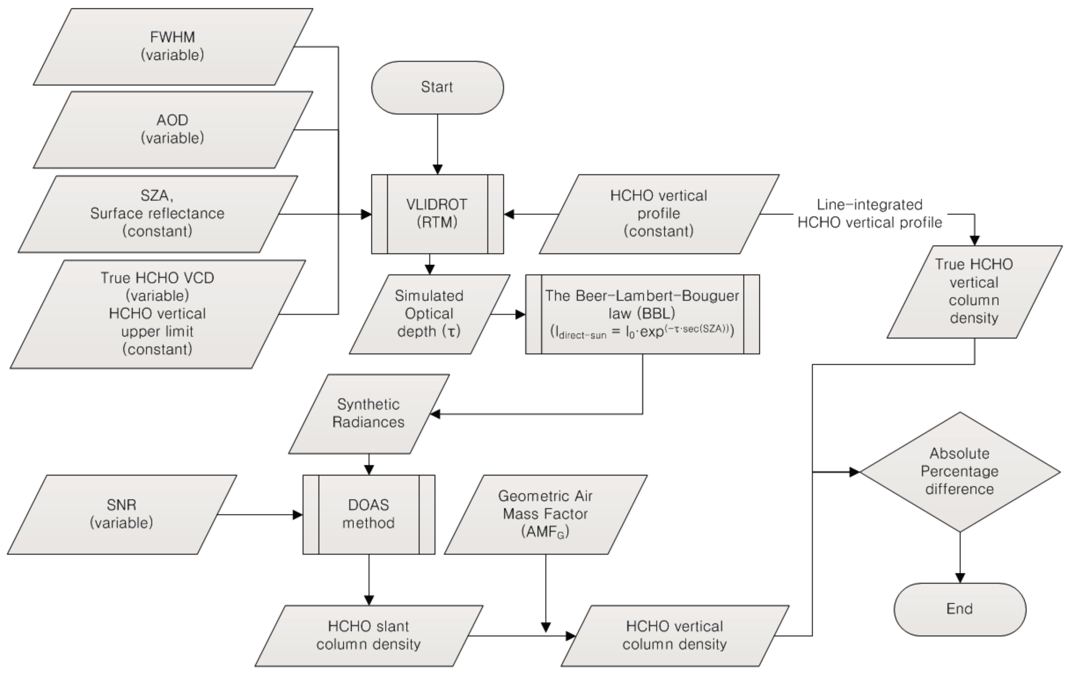
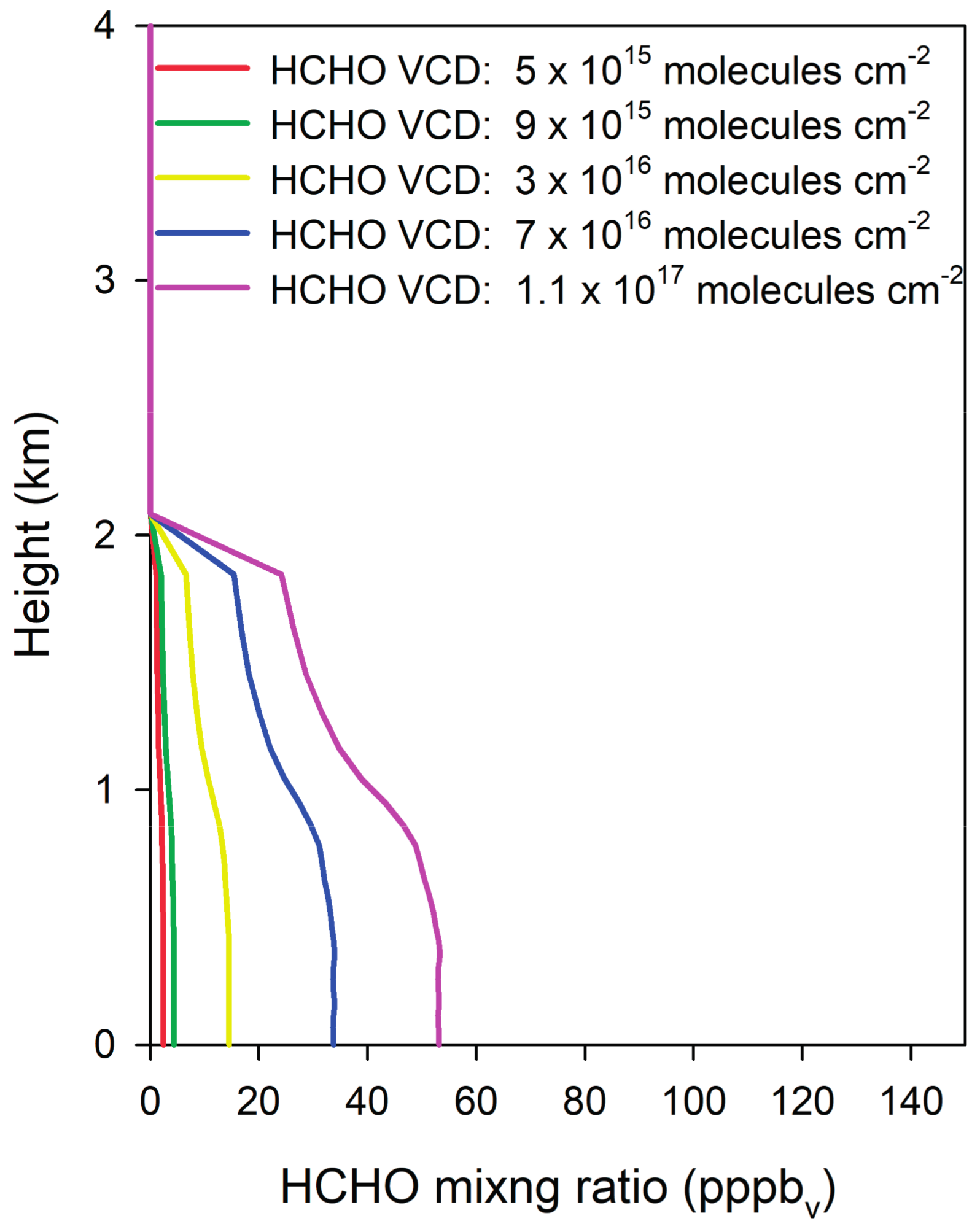
2.1. Estimation of HCHO_VCD Retrieval Accuracy

Figure 1 shows a flowchart of the HCHO_VCD retrieval accuracy test. We used a four-step process to determine which parameters affect the HCHO_VCD retrieval accuracy. First, a total 135 of synthetic radiances were generated using the linearized pseudo-spherical scalar and vector discrete ordinate radiative transfer (VLIDORT, version 2.6) model [29] between 290 and 510 nm and with a 0.2 nm sampling resolution under various SNR, FWHM, AOD, and HCHO_VCD. Here, the HCHO vertical profile was assumed to be a box profile [30] (Figure 2). The values of the HCHO_VCD and HCHO vertical upper limit, model input parameters such as aerosol properties (aerosol type, AOD, and aerosol peak height (APH)), and the geometry information (solar zenith angle (SZA) and surface reflectance) are summarized in

Table 2. Variables and constant used to calculate synthetic radiances.

Variable	Value	Constant	Value
HCHOVCD (molecules cm−2)	$5\times {10}^{15}$ $9\times {10}^{15}$ $3\times {10}^{16}$ $7\times {10}^{16}$ $1.1\times {10}^{17}$	Surface reflectance	0.04
		SZA	30°
		Aerosol Type	Smoke Type
AOD	0.2, 0.6, and 1.5	APH (km)	0
SNR	650, 920, and 1300	HCHO Vertical Upper Limit (km)	2
FWHM (nm)	0.2, 0.6, and 1.0

. Other gas vertical profiles, such as ozone (O₃) and nitrogen dioxide (NO₂), were obtained from the Deriving Information of Surface Conditions from Column and Vertically Resolved Observations Relevant to Air Quality (Discover-AQ) dataset [31,32].

The aerosol profile is based on a Gaussian distribution function (GDF), as used by Jeong et al. [33] and Hong et al. [34], and the GDF equation is as follows:

$$\mathrm{GDF}={{\displaystyle \int }}_{z_{n1}}^{z_{n2}}W\frac{e^{-h\left(z-z_p\right)}}{{\left[1+e^{-h\left(z-z_p\right)}\right]}^2}dz$$

(1)

$$\mathsf{\eta }=\frac{\ln \left(3+\sqrt{8}\right)}{h}$$

(2)

where $z_{n1}$ and $z_{n2}$ are the aerosol lower and upper limits, respectively, W is a normalization constant related to total aerosol loading, h is related to the half width $\mathsf{\eta }$, and $z_p$ is the APH [29,33,34].

Second, random noise (SNR from 650, 920, and 1300) was added to the simulated synthetic radiances. Herman et al. [25] reported that the Pandora spectrometer system is not noise limited when measuring under clear-sky conditions [25]. Moreover, Herman et al. [25] assume that, if the entire variability were instrument noise, the signal-to-noise ratio would be 650:1. SNRs of 920 and 1300 calculated when the exposure time is doubled and quadrupled, respectively. These synthetic radiances were convolved using various Gaussian slit functions with a full-width-half-maximums (FWHMs) of 0.2, 0.6, and 1.0. The SNR of each synthetic radiance was calculated using the following equation [35]:

$$SN{R}_i\left(\mathsf{\lambda }\right)=SN{R}_a\sqrt{\frac{I_i\left(\mathsf{\lambda }\right)}{I_a}}$$

(3)

where $SN{R}_i\left(\mathsf{\lambda }\right)$ and $I_i\left(\mathsf{\lambda }\right)$ are the i-th SNR and radiance at wavelength $\mathsf{\lambda }$, respectively, $I_a$ is the average value of all synthetic radiances from 290 to 510 nm, and $SN{R}_a$ is its corresponding SNR.

Third, in the present study, the AMF_G was used as the AMF because Pandora takes ground-based direct-sun measurements [25]. The AMF_G is calculated as follows:

$$AM{F}_G=\sec \left(SZA\right).$$

(4)

Then, the retrieved HCHO Slant Column Densities (HCHO_SCDs) were divided by the AMF_G to convert them to HCHO_VCD values. The spectral fitting method used to retrieve HCHO_SCD is described in Section 2.2.2.

Finally, the retrieved HCHO_VCD values were compared with the true HCHO_VCD values. Here, the true HCHO_VCD denotes the line-integrated value of the HCHO vertical profile data, which are inputted in the RTM to calculate the synthetic radiances (Figure 1). The absolute percentage difference (APD) was calculated through the difference between the true HCHO_VCD retrieved from the HCHO vertical profile, which are inputted in the RTM to calculate the synthetic radiances and the HCHO_VCD retrieved by the spectral fitting method and AMF_G described above. The HCHO_VCD error, which is the difference between the retrieved and true HCHO_VCD values, occurs only due to the spectral fitting because we used AMF_G values in this study.

2.2. Description of Pandora Measurements and Additional Datasets

2.2.1. Pandora Measurements

The Pandora measurements were made on the rooftop of the Science Building at Yonsei University in Seoul (37.56$°$N, 126.94$°$E) between March 2012 and December 2014. The PSI consists of a two filter wheel optical head sensor mounted on a computer-controlled sun tracker and sky scanner connected via a 400-micron core diameter single-strand multi-mode optical fiber to an Avantes symmetric Czerny-Turner 2048 × 64 pixels charge-coupled device (CCD) detector maintained at a temperature of 1 °C to reduce the dark current noise. This spectrometer operates in the 280–530 nm spectral range with a 0.6 nm slit function width (full width at half maximum). A fiber optic cable allows the temperature-sensitive spectrometer to be stored away from the sun in an insulated box equipped with a thermoelectric heating and cooling system that maintains the temperature within ±1 °C of 20 °C. The sensor head has a multiply baffled collimating tube with a 1.6° FOV (field of view). Light passing through the collimator then passes through a filter wheel assembly that contains the two UV band-pass filters (280–320 and 280–380 nm) used for SO₂ and O₃ measurements, respectively, an open hole, and a blocked region for measuring the dark current after each measurement. In addition, there is a circuit board for controlling the filter wheel and a sun-tracking device connected through an RS-232 serial computer interface. A flat quartz window constitutes the first optical element, which protects the intimal optical and electrical components from rain, dust, and humidity. Herman et al. [24,25] provided a detailed description of the instrument.

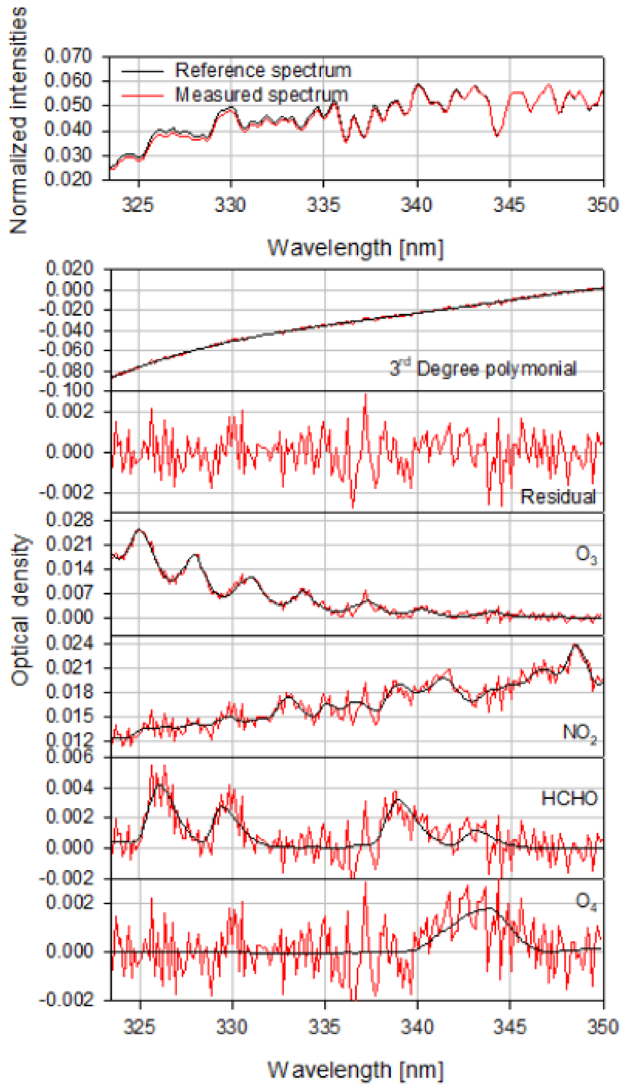
2.2.2. Spectral Analysis (Retrieval of HCHO Slant Column Density)

To derive the slant column density (SCD) of HCHO (HCHO_SCD), we analyzed the PSI data using QDOAS software [36], which is based on difference optical absorption spectroscopy (DOAS) [37,38]. The noise signals, including the dark current and offset signals from the Pandora CCD detector, were recorded during each measurement routine and then removed from the direct sunlight spectra. The wavelengths of the spectra recorded by the Pandora system were calibrated by fitting the raw spectra to a solar reference spectrum [39]. The DOAS fitting was carried out over the wavelength interval (332.5–350 nm). This spectral interval, with three strong HCHO absorption bands, was found to have the smallest fitting residual. A spectrum recorded at ~12:00 p.m. LT on 9 September was used as the reference spectrum (RS). The minimum HCHO_SCD was calculated from the RS via DOAS spectral fitting. The RS and the absorption cross sections of HCHO, NO₂, O₃, and O₄ were simultaneously fitted to the measurement spectra using a nonlinear least squares method [37,38] and QDOAS software. We used the HCHO absorption cross section [40], NO₂ absorption cross sections (220 K and 296 K; [41]), O₃ absorption cross sections (223 K and 243 K; [42]), and the O₄ absorption cross section [43] to perform the DOAS fitting. The BrO absorption cross section was excluded from the spectral fitting since no (or negligible) BrO absorption features were found during the spectral fitting process. All reference absorption cross-sectional spectra were convolved with the measured Pandora slit function. The NO₂ and O₃ spectra were I_o-corrected using QDOAS software. We used the third-order polynomial to eliminate the effects of Rayleigh and Mie scattering.

Figure 3 shows an example of the deconvolution of the DOAS spectrum that was used to evaluate the HCHO_SCD at 12:00 p.m. LT on 13 March 2012. Finally, the HCHO_SCD obtained from the DOAS technique was converted to the HCHO_VCD by dividing the SCD by the AMF_G (described in Section 2.1).

2.2.3. Ozone Monitoring Instrument (OMI) Data

To compare the Pandora HCHO_VCD values with those from the OMI measurements, we used the OMI/Aura HCHO total column global 0.25° latitude/longitude grid (V003) HCHO level 2G data [44]. The OMI is onboard NASA’s Earth Observing System (EOS)/Aura satellite [45] that was launched on 15 July 2004 into a sun-synchronous ascending polar orbit at an altitude of 705 km and with a local equator crossing time of 1:45 p.m. A detailed description of the OMI HCHO algorithm can be found in Chance [46]. The OMI HCHO data used here were cloud-free (cloud fraction < 0.2) and flagged as “0” (quality flag = 0), which indicates a good quality level [47,48]. The use of quality flagged as “0” only uses the data that passes all quality checks including the row anomaly.

Table 3. Ozone monitoring instrument (OMI) data and flags considered.

Product Name	Filter Flags and Conditions
HCHO (OMHCHOG)	Cloud fraction > 0.2 Solar zenith angle > 70° Suspect (quality flag = 1) Bad (quality flag = 2) Missing (quality flag ≤ −1)

summarizes the product name, filter flags, and the condition of the OMI HCHO product that we used [47].

We used the Pandora and OMI data in the cloud-free condition, which is determined on the basis of the cloud observation data [49] of the Korea Meteorological Administration (KMA) and the OMI cloud data (cloud fraction < 0.2; quality flag = 0) [47,48].

3. Results

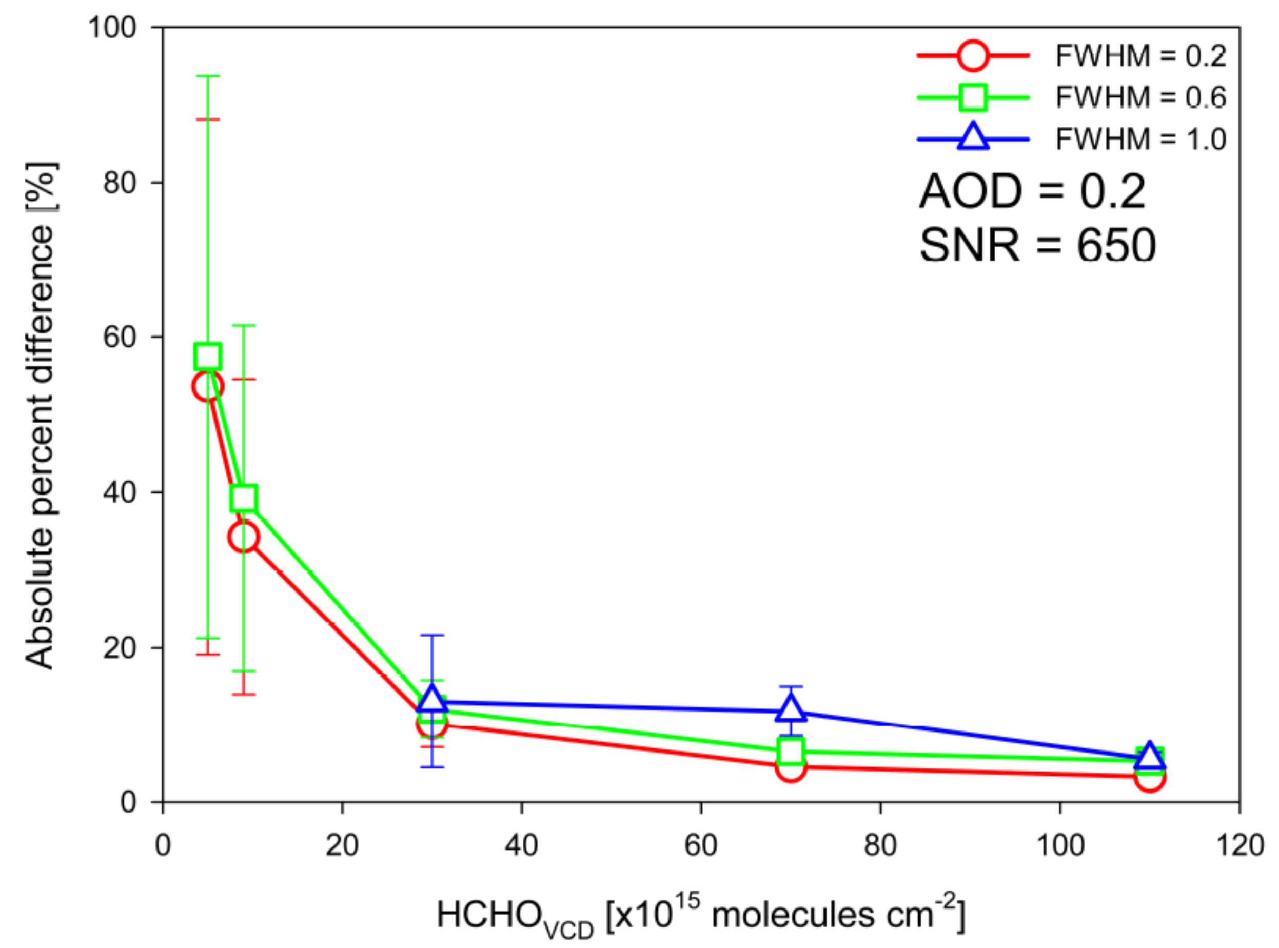
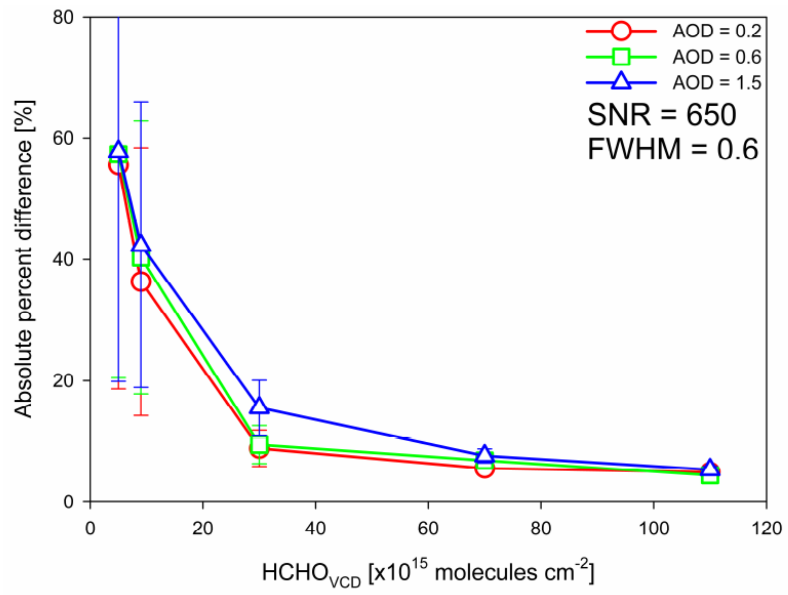
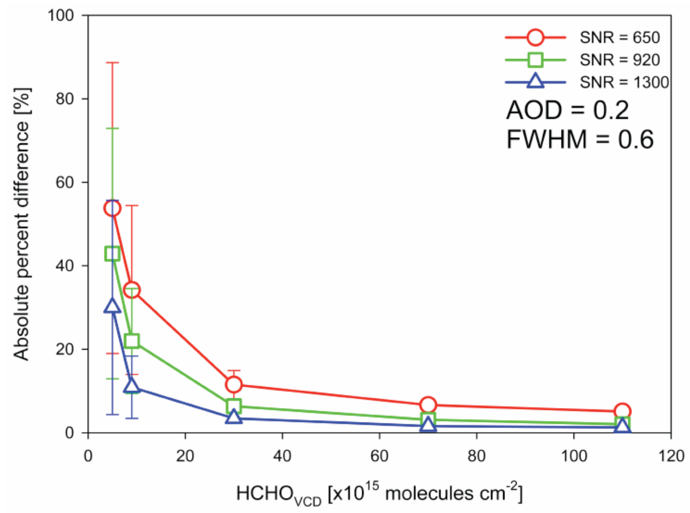
3.1. HCHO Precision Estimations

To investigate the effects of SNR, slit function (FWHM), and AOD on the accuracy on the HCHO_VCD values obtained from the ground-based direct-sun measurements, the HCHO SCDs were retrieved using the DOAS method from synthetic radiances. The retrieved SCDs were converted into VCDs by divided them by the AMF_G (described in Section 2.1), which we assumed to have no errors.

Figure 4 shows the APD between the true and retrieved HCHO_VCD values as a function of HCHO_VCD values under various SNR conditions (SNRs of 650, 920, and 1300) with an FWHM of 0.6 nm and an AOD of 0.2. A significant increase in the APDs was found for the HCHO_VCD values less than 3 × 10¹⁶ molecules cm⁻² (molec. cm⁻²). In particular, when SNR = 650, the APDs were found to be larger than those of high SNR conditions (SNR = 920 and 1300). In Figure 4, for an SNR of 1300, the APD ranges from 1 to 3% for HCHO_VCD values equal to or greater than 3 × 10¹⁶ molec. cm⁻², whereas the APD is between 3 and 30% for HCHO_VCD values less than 3 × 10¹⁶ molec. cm⁻². However, the APD for an SNR of 650 ranges from 5 to 11% for HCHO_VCD values equal to or greater than 3 × 10¹⁶ molec. cm⁻², whereas the APD is between 11 and 53% for HCHO_VCD values less than 3 × 10¹⁶ molec. cm⁻².

Figure 5 shows the slit function (FWHM) effects as a function of HCHO_VCD values for an SNR of 650. The effects of small and large FWHM values on the APD are found to be small. The APDs of FWHM 0.2 (0.6) ranges from 3 (5%) to 10% (12%) for HCHO_VCD values equal to or greater than 3 × 10¹⁶ molec. cm⁻² and ranges from 10 (12%) to 53% (57%) for HCHO_VCD values less than 3 × 10¹⁶ molec. cm⁻². The average APD of all three FWHM (0.2, 0.6, and 1.0) conditions is 8% for HCHO_VCD values equal to or greater than 3 × 10¹⁶ molec. cm⁻², while it is 46% for HCHO_VCD values less than 3 × 10¹⁶ molec. cm⁻². The APDs were not calculated for HCHO_VCD values of 5 × 10¹⁵ and 9 × 10¹⁵ molec. cm⁻² at an FWHM of 1.0 due to the spectral fitting failure.

Figure 6 shows the effect of AOD variation as a function of HCHO_VCD values for an SNR = 650, SZA = 30, and FWHM = 0.6. An increasing AOD leads to an increase in APD. For an AOD of 0.2, the APD ranges from 4 to 8% when HCHO_VCD values are equal to or greater than 3 × 10¹⁶ molec. cm⁻². However, the APD is between 8 and 55% when HCHO_VCD values are less than 3 × 10¹⁶ molec. cm⁻². For an AOD of 0.6 (1.0), the APD ranges from 4 (5%) to 9% (15%) when HCHO_VCD values are equal to or greater than 3 × 10¹⁶ molec. cm⁻². However, the APD is between 9 (15%) and 57% (57%) when the HCHO_VCD values are less than 3 × 10¹⁶ molec. cm⁻². For the small HCHO_VCD values (5 × 10¹⁵ molec. cm⁻²), the APD of low AOD (AOD = 0.2) was found to be similar to that of high AOD (AOD = 1.5), which implies that the large noise associated with the poor SNR (650) dominantly influences the APD compared to the AOD effect for the small HCHO_VCD values. As shown in Figure 5, we found that the APDs are similar between the various FWHM values at the poor SNR condition (650), which supports that the large noise with the poor SNR is dominant on the APD for the small HCHO_VCD values. Meanwhile, for the large HCHO_VCD values (1.1 × 10¹⁷ molec. cm⁻²), the APD of low AOD (AOD = 0.2) was found to be similar to that of high AOD (AOD = 1.5), which implies that the sensitivity of the Pandora to this high HCHO_VCD value was so great that the AOD effect was negligible. Therefore, we found, interestingly, that the maximum AOD effect on HCHO accuracy for the HCHO_VCD value was 3.0 × 10¹⁶ molecules cm⁻², for which both the noise effect at small HCHO_VCD values and the high sensitivity effect at high HCHO_VCD values are minimal.

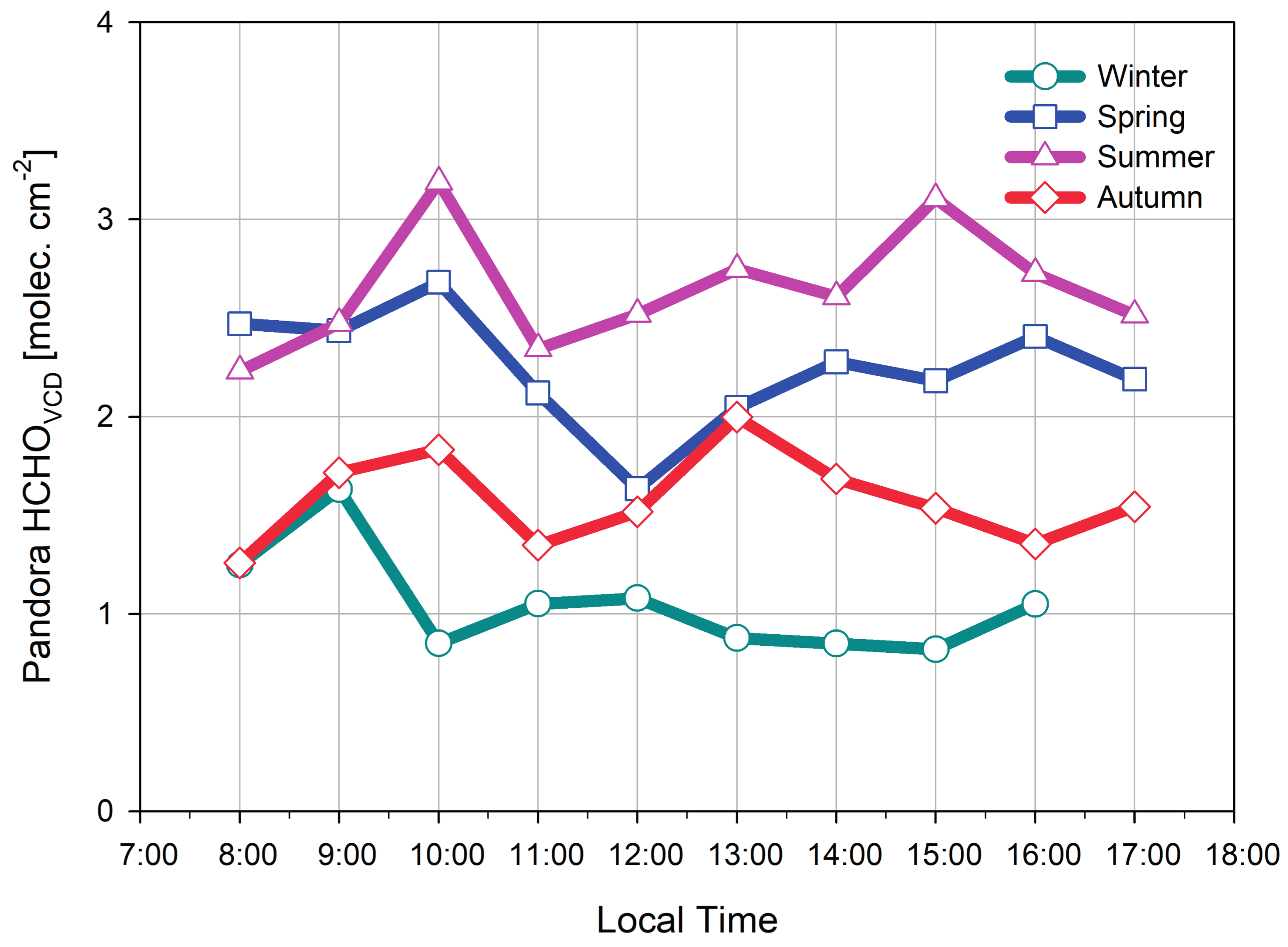
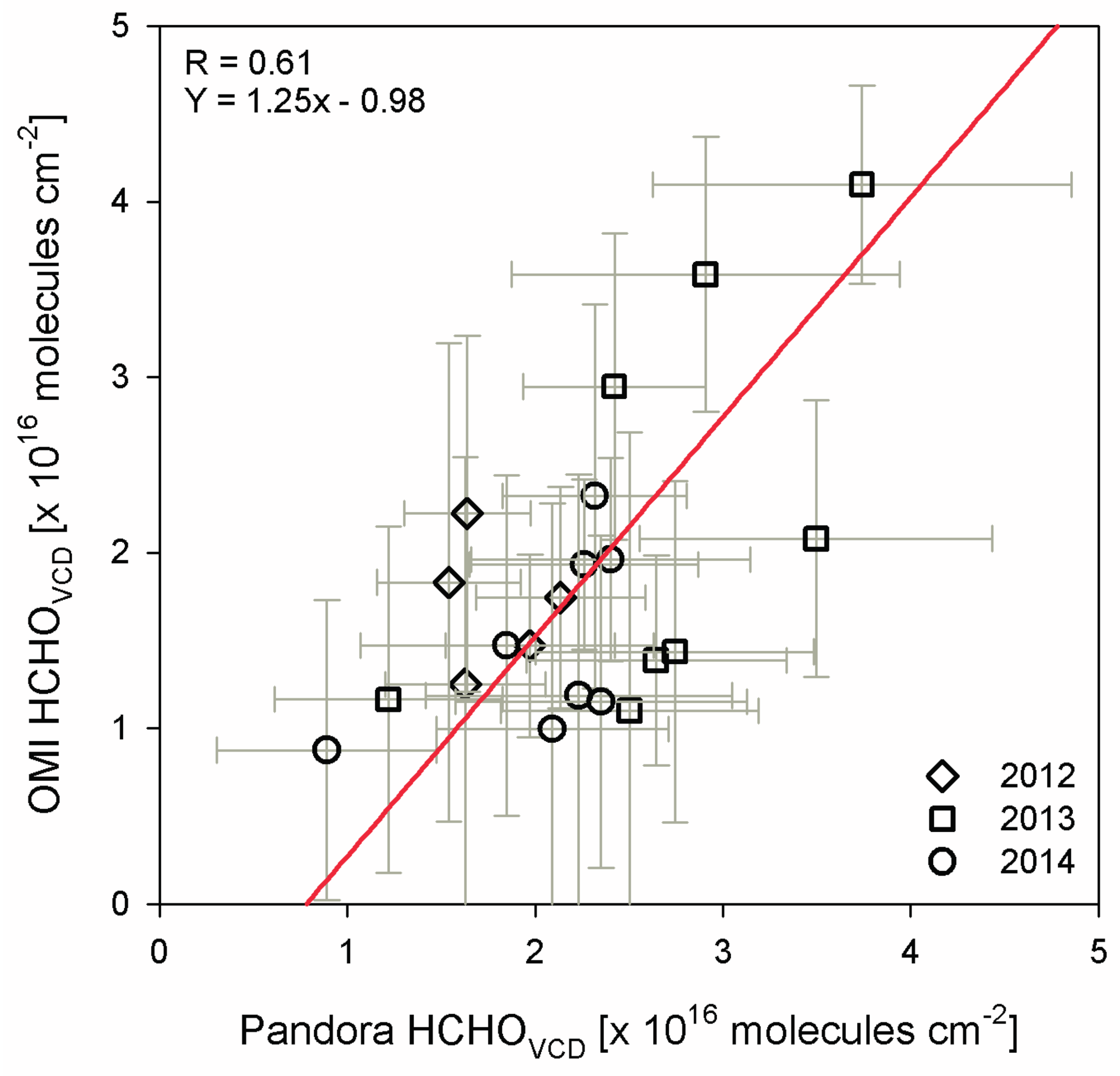
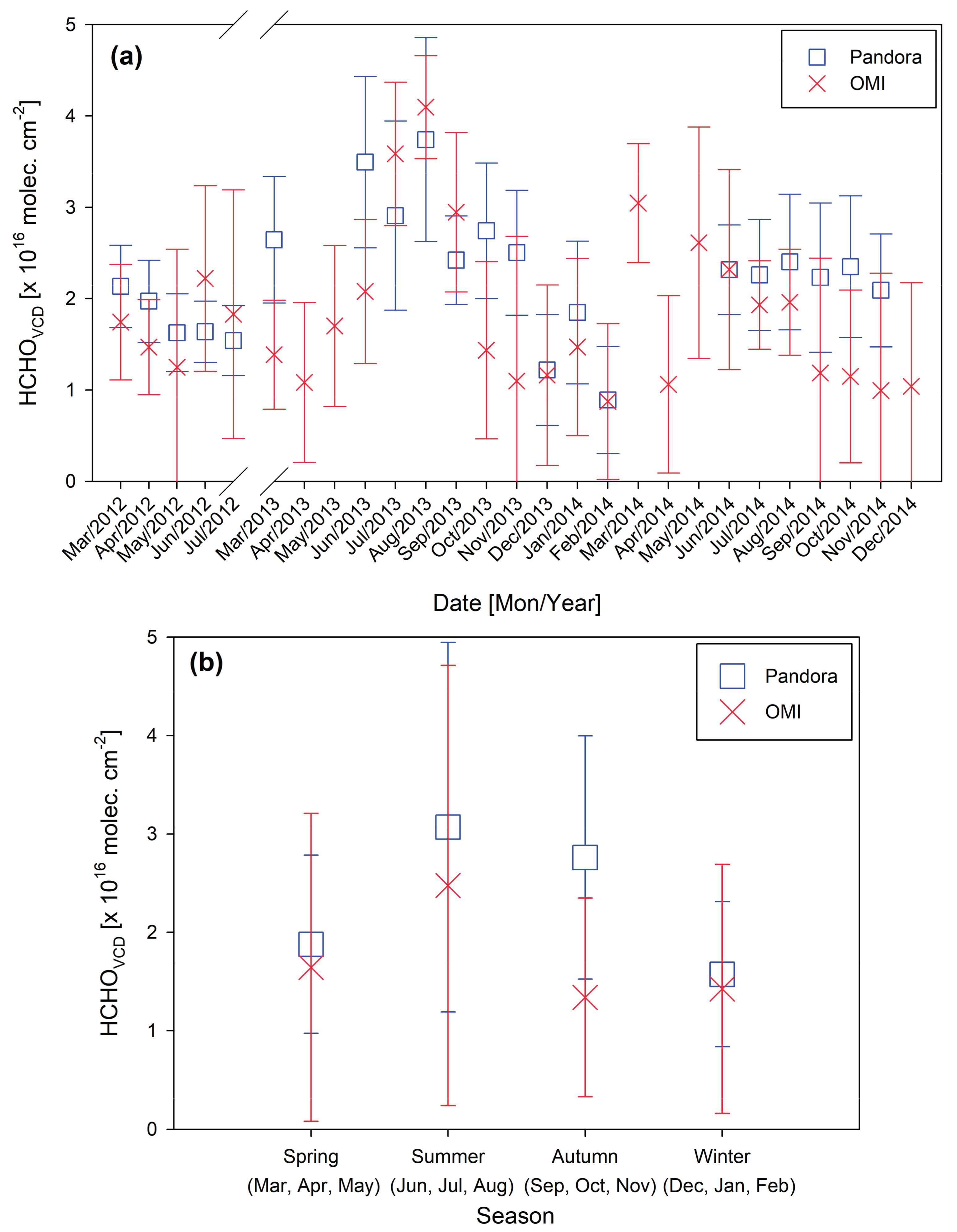
3.2. HCHO_VCD Retrieval in Seoul Using Pandora

Figure 7 shows the diurnal variations in HCHO_VCD for each season based on the Pandora data from Seoul. The maximum (minimum) values of Pandora HCHO_VCD were 2.68 × 10¹⁶ (1.63 × 10¹⁶), 3.19 × 10¹⁶ (2.23 × 10¹⁶), 2.00 × 10¹⁶ (1.26 × 10¹⁶), and 1.63 × 10¹⁶ (0.82 × 10¹⁶) molec. cm⁻² for spring, summer, autumn, and winter, respectively. Figure 7 shows that the Pandora HCHO_VCD value tends to be high between 9:00 and 10:00 a.m. in the morning in all seasons. We interpret these high Pandora HCHO_VCD levels in Seoul in the morning to be associated with significant increases in the emissions of volatile organic compounds (VOCs) and their subsequent photo-oxidation from traffic during the rush hour. A small contribution may also be derived from direct HCHO emissions during this time [51]. The Pandora HCHO_VCD is low throughout the late morning between 10:00 a.m. and 12:00 p.m. LT in all seasons. An increase in HCHO_VCD is also evident in Figure 7 sometime in the afternoon for all seasons except winter, but the specific time varies with the season (i.e., 2:00 p.m. in spring, 3:00 p.m. in summer, and 1:00 p.m. in autumn). These increases in all seasons except winter can be attributed to the photolysis of VOCs and hydrocarbon photo-oxidation by the OH${}^{\bullet }$ radical and ozone [52]. However, there is no peak on winter afternoons, possibly due to the weak UV solar radiation at that time, even in the afternoon, and an increase in wind speed compared with the summer.

The diurnal pattern of Pandora HCHO_VCD shown in Figure 7 is similar to that of the HCHO mixing ratio near the ground seen in the MAX-DOAS and Long-Path DOAS (LP-DOAS) measurements from several cities including Seoul and Beijing [52,53,54]. However, previous studies [55,56] have reported high HCHO levels at noon and low HCHO levels in the morning from the Houston–Galveston Airshed (HGA) and Southern China, which are opposite to the diurnal pattern found in Seoul in this study. As discussed in [52], the different diurnal variations of HCHO seen among various urban areas might be related to differences in the HCHO sources and loss mechanisms at each site.

Figure 8 shows the monthly (Figure 8a) and seasonally averaged (Figure 8b) variations in the Pandora HCHO_VCD and OMI HCHO_VCD from Seoul during the study period when both OMI HCHO column and Pandora HCHO data are available, and the error bars represent the calculated HCHO_VCD uncertainties for each measurement. The monthly Pandora HCHO_VCD values were unavailable for some months due to instrument malfunctions. Figure 8 shows that both the Pandora HCHO_VCD and OMI HCHO_VCD are high in summer, whereas they are low in winter, with similar HCHO_VCD patterns in both the Pandora and OMI data. This high-in-summer, low-in-winter pattern of HCHO_VCD implies that the solar radiation energy leads to photo-oxidation that plays a key role in the seasonal HCHO pattern in Seoul. Biogenic species, especially isoprene, may also influence the seasonal HCHO pattern in Seoul. The monthly and seasonal HCHO patterns in Seoul are similar to those reported previously [52,53] in studies carried out in urban areas.

Figure 9 shows a scatter plot of the monthly Pandora and OMI HCHO_VCD levels from Seoul between 2012 and 2014. To determine the Pandora HCHO_VCD retrieval errors, we calculated the error covariance of the spectral fitting errors, but with no errors associated with the direct-sun AMF_G calculation (Figure 8 and Figure 9). Then, the error covariance was used in the error propagation equation [17,50]. The error bars of the OMI HCHO_VCD in Figure 9 were obtained from the OMI Level 2G product. The HCHO retrieval uncertainty of the OMI Level 2G product varies between 50 and 105% (https://www.cfa.harvard.edu/atmosphere/Instruments/OMI/PGEReleases/READMEs/OMHCHO_README_v3.0.pdf). In Figure 9, the average spectral fitting error of the Pandora (OMI) data was 85% (157%). Given the Pandora SNR of 950 in Seoul and the HCHO_VCD interval in Figure 9, the APD may range from 11 to 34%, as shown in Figure 4. Nevertheless, the correlation coefficient (R) between the Pandora HCHO_VCD and OMI HCHO_VCD was 0.61, with a slope of 1.25. The Pandora HCHO_VCD values generally tend to be larger than those of the OMI HCHO_VCD (Figure 9) over the study period of 2012–2014. This tendency for the Pandora HCHO_VCD values to be greater than the OMI HCHO_VCD values could be associated with differences in the sensitivities as well as bias to the true HCHO value between the ground-based Pandora and satellite-based OMI instruments. We found a positive bias trend in the Pandora HCHO_VCD to the true HCHO value, which is partly in agreement with the tendency for the Pandora HCHO_VCD values to be greater than the OMI HCHO_VCD values in Figure 9, if we assume that the OMI HCHO_VCD is true. However, in order to identify the reasons for the relationship between the HCHO_VCD values retrieved from Pandora and OMI in Figure 9, additional synthetic and field validation studies need to be carried out to understand the information, such as the accuracy and bias of the OMI HCHO measurements.

4. Discussion

To use a ground-based instrument as a tool to validate satellite products, the accuracy of the data obtained from the ground-based instrument need to be quantified and understood. In the present study, we quantified the accuracy of DOAS HCHO retrieval using ground-based direct-sun measurements. The most important finding of this HCHO accuracy study was that the APDs always significantly increase for HCHO_VCD values less than 3 × 10¹⁶ molec. cm⁻² under various SNR, FWHM, and AOD conditions. The APD of a low SNR (SNR = 650) is much larger than that of a high SNR (SNR = 1300) for HCHO_VCD values less than 3 × 10¹⁶ molec. cm⁻². When Pandora HCHO data are compared to those of satellite data, one should be aware that the HCHO_VCD error may be larger than about 55% in the condition of SNR = 650. In order to enhance Pandora HCHO accuracy, especially over low HCHO conditions less than 2 × 10¹⁶ molec. cm⁻², the SNR of the Pandora needs to be increased to 1300. For example, as the SNR increases from 650 to 1300, the average APD decreases from 53 (34%) to 30% (10%) under the HCHO_VCD of 5 × 10¹⁵ (9 × 10¹⁵) molec. cm⁻².

In addition, we retrieved the HCHO_VCD values using Pandora in a megacity and here report its diurnal and seasonal variations. The diurnal variation found in the present study is similar to that of the HCHO mixing ratio near the ground seen in the MAX-DOAS and Long-Path DOAS (LP-DOAS) measurements in Seoul and Beijing [52,53,54]. However, Pang et al. [55] and Rappenglück et al. [56] reported high HCHO levels at noon and low HCHO levels in the morning from the Houston–Galveston Airshed (HGA) and Southern China, which are different from the diurnal characteristics found in Seoul in the present study. As discussed by Lee et al. [52], the different diurnal variations of HCHO seen among various urban areas might be related to differences in the HCHO sources and loss mechanisms at each site. These high-in-summer, low-in-winter patterns found in both Pandora and OMI HCHO_VCD values in Seoul are similar to those reported by Lee et al. [52] and Pang et al. [53] carried out in Seoul and Beijing. The HCHO_VCD and its temporal pattern reported in the present study are thought to be useful in validating the HCHO_VCD data produced by both satellite observations and CTMs, since the temporal characteristics of HCHO_VCD values are different among observations sites.

5. Conclusions

In the present study, for the first time, we investigate the sensitivity of HCHO retrieval under various SNR, FWHM, AOD, and HCHO_VCD conditions based on ground-based direct-sun measurement. Increasing SNR leads to a significant increase in the APD under various AOD and FWHM conditions. In a high-HCHO condition (HCHO_VCD = 1.1 × 10¹⁷ molec. cm⁻²) and a low-HCHO condition (HCHO_VCD = 5.0 × 10¹⁵ molec. cm⁻²), the APD of low AOD (AOD = 0.2) is found to be similar to that of high AOD (AOD = 1.5). We found the maximum AOD effect when the HCHO_VCD is 3.0 × 10¹⁶ molec. cm⁻². In terms of first-time HCHO measurements using Pandora, the HCHO_VCD tends to be higher in the morning (9:00 a.m.–10:00 a.m. LT) but lower through the late morning (10:00 a.m.–12:00 p.m. LT) in all seasons in Seoul. An increase in HCHO_VCD occurred in the afternoon for all seasons except winter. Both Pandora HCHO_VCD and OMI HCHO are high in summer and low in winter. The correlation coefficient between Pandora HCHO_VCD and OMI HCHO_VCD is 0.61. The Pandora HCHO_VCD values generally tend to be larger than those derived from the OMI observations.

References

1. Logan, J.A.; Prather, M.J.; Wofsy, S.C.; McElroy, M.B. Tropospheric chemistry: A global perspective. J. Geophys. Res. Oceans 1981, 86, 7210–7254. [Google Scholar] [CrossRef]
2. Jiménez, R.; Martilli, A.; Balin, I.; Van den Bergh, H.; Calpini, B.; Larsen, B.; Favaro, G.; Kita, D. Measurement of Formaldehyde (HCHO) by DOAS: Intercomparison to DNPH Measurements and Interpretation from Eulerian Model Calculations. In Proceedings of the A&WMA 93rd Annual Conference, Salt Lake City, UT, USA, 18–22 June 2000. [Google Scholar]
3. Hak, C.; Pundt, I.; Trick, S.; Kern, C.; Platt, U.; Dommen, J.; Ordóñez, C.; Prévôt, A.; Junkermann, W.; Astorga-Lloréns, C. Intercomparison of four different in-situ techniques for ambient formaldehyde measurements in urban air. Atmos. Chem. Phys. 2005, 5, 2881–2900. [Google Scholar] [CrossRef]
4. Jones, N.; Riedel, K.; Allan, W.; Wood, S.; Palmer, P.; Chance, K.; Notholt, J. Long-term tropospheric formaldehyde concentrations deduced from ground-based fourier transform solar infrared measurements. Atmos. Chem. Phys. 2009, 9, 7131–7142. [Google Scholar] [CrossRef]
5. Neitzert, V.; Seiler, W. Measurement of formaldehyde in clean air. Geophys. Res. Lett. 1981, 8, 79–82. [Google Scholar] [CrossRef]
6. Tanner, R.L.; Meng, Z. Seasonal variations in ambient atmospheric levels of formaldehyde and acetaldehyde. Environ. Sci. Technol. 1984, 18, 723–726. [Google Scholar] [CrossRef]
7. Harris, G.; Mackay, G.; Iguchi, T.; Mayne, L.; Schiff, H. Measurements of formaldehyde in the troposphere by tunable diode laser absorption spectroscopy. J. Atmos. Chem. 1989, 8, 119–137. [Google Scholar] [CrossRef]
8. Grosjean, D.; Williams, E.L.; Seinfeld, J.H. Atmospheric oxidation of selected terpenes and related carbonyls: Gas-phase carbonyl products. Environ. Sci. Technol. 1992, 26, 1526–1533. [Google Scholar] [CrossRef]
9. Arlander, D.; Cronn, D.; Farmer, J.; Menzia, F.; Westberg, H. Gaseous oxygenated hydrocarbons in the remote marine troposphere. J. Geophys. Res. Atmos. 1990, 95, 16391–16403. [Google Scholar] [CrossRef]
10. Heikes, B.G. Formaldehyde and hydroperoxides at Mauna Loa observatory. J. Geophys. Res. Atmos. 1992, 97, 18001–18013. [Google Scholar] [CrossRef]
11. Zhou, X.; Lee, Y.N.; Newman, L.; Chen, X.; Mopper, K. Tropospheric formaldehyde concentration at the Mauna Loa observatory during the Mauna Loa observatory photochemistry experiment 2. J. Geophys. Res. Atmos. 1996, 101, 14711–14719. [Google Scholar] [CrossRef]
12. Ayers, G.; Gillett, R.; Granek, H.; De Serves, C.; Cox, R. Formaldehyde production in clean marine air. Geophys. Res. Lett. 1997, 24, 401–404. [Google Scholar] [CrossRef]
13. Chance, K.V.; Palmer, P.I.; Spurr, R.J.; Martin, R.V.; Kurosu, T.P.; Jacob, D.J. Satellite observations of formaldehyde over North America from GOME. Geophys. Res. Lett. 2000. [Google Scholar] [CrossRef]
14. De Smedt, I.; Müller, J.-F.; Stavrakou, T.; Van Der, A.R.; Eskes, H.; Van Roozendael, M. Twelve years of global observations of formaldehyde in the troposphere using GOME and SCIAMACHY sensors. Atmos. Chem. Phys. 2008, 8. [Google Scholar] [CrossRef]
15. De Smedt, I.; Stavrakou, T.; Hendrick, F.; Danckaert, T.; Vlemmix, T.; Pinardi, G.; Theys, N.; Lerot, C.; Gielen, C.; Vigouroux, C. Diurnal, seasonal and long-term variations of global formaldehyde columns inferred from combined OMI and GOME-2 observations. Atmos. Chem. Phys. 2015, 15, 12519–12545. [Google Scholar] [CrossRef]
16. Li, X.; Brauers, T.; Hofzumahaus, A.; Lu, K.; Li, Y.; Shao, M.; Wagner, T.; Wahner, A. MAX-DOAS measurements of NO2, HCHO and CHOCHO at a rural site in Southern China. Atmos. Chem. Phys. 2013, 13, 2133–2151. [Google Scholar] [CrossRef]
17. Lee, H.; Ryu, J.; Irie, H.; Jang, S.-H.; Park, J.; Choi, W.; Hong, H. Investigations of the Diurnal Variation of Vertical HCHO Profiles Based on MAX-DOAS Measurements in Beijing: Comparisons with OMI Vertical Column Data. Atmosphere 2015, 6, 1816–1832. [Google Scholar] [CrossRef]
18. Franco, B.; Hendrick, F.; Van Roozendael, M.; Müller, J.-F.; Stavrakou, T.; Marais, E.; Bovy, B.; Bader, W.; Fayt, C.; Hermans, C. Retrievals of formaldehyde from ground-based FTIR and MAX-DOAS observations at the Jungfraujoch station and comparisons with GEOS-Chem and IMAGES model simulations. Atmos. Meas. Tech. 2015, 8, 1733–1756. [Google Scholar] [CrossRef]
19. Heckel, A.; Richter, A.; Tarsu, T.; Wittrock, F.; Hak, C.; Pundt, I.; Junkermann, W.; Burrows, J. MAX-DOAS measurements of formaldehyde in the Po-Valley. Atmos. Chem. Phys. 2005, 5, 909–918. [Google Scholar] [CrossRef]
20. Vigouroux, C.; Hendrick, F.; Stavrakou, T.; Dils, B.; Smedt, I.D.; Hermans, C.; Merlaud, A.; Scolas, F.; Senten, C.; Vanhaelewyn, G. Ground-based FTIR and MAX-DOAS observations of formaldehyde at Réunion Island and comparisons with satellite and model data. Atmos. Chem. Phys. 2009, 9, 9523–9544. [Google Scholar] [CrossRef]
21. Irie, H.; Takashima, H.; Kanaya, Y.; Boersma, K.; Gast, L.; Wittrock, F.; Brunner, D.; Zhou, Y.; Roozendael, M.V. Eight-component retrievals from ground-based MAX-DOAS observations. Atmos. Meas. Tech. 2011, 4, 1027–1044. [Google Scholar] [CrossRef] [Green Version]
22. Peters, E.; Wittrock, F.; Großmann, K.; Frieß, U.; Richter, A.; Burrows, J. Formaldehyde and nitrogen dioxide over the remote western Pacific Ocean: SCIAMACHY and GOME-2 validation using ship-based MAX-DOAS observations. Atmos. Chem. Phys. 2012, 12, 11179–11197. [Google Scholar] [CrossRef] [Green Version]
23. Pinardi, G.; Van Roozendael, M.; Abuhassan, N.; Adams, C.; Cede, A.; Clémer, K.; Fayt, C.; Frieß, U.; Gil, M.; Herman, J. MAX-DOAS formaldehyde slant column measurements during CINDI: Intercomparison and analysis improvement. Atmos. Meas. Tech. 2013, 6, 167. [Google Scholar] [CrossRef]
24. Herman, J.; Cede, A.; Spinei, E.; Mount, G.; Tzortziou, M.; Abuhassan, N. NO2 column amounts from ground-based Pandora and MFDOAS spectrometers using the direct-Sun DOAS technique: Intercomparisons and application to OMI validation. J. Geophys. Res. Atmos. 2009, 114. [Google Scholar] [CrossRef]
25. Herman, J.; Evans, R.; Cede, A.; Abuhassan, N.; Petropavlovskikh, I.; McConville, G. Comparison of ozone retrievals from the Pandora spectrometer system and Dobson spectrophotometer in Boulder, Colorado. Atmos. Meas. Tech. 2015, 8, 3407–3418. [Google Scholar] [CrossRef]
26. Fioletov, V.E.; McLinden, C.A. Sulfur dioxide (SO2) vertical column density measurements by Pandora spectrometer over the Canadian oil sands. Atmos. Meas. Tech. 2016, 9, 2961. [Google Scholar] [CrossRef]
27. Volkamer, R.; Coburn, S.; Dix, B.; Sinreich, R. MAX-DOAS observations from ground, ship, and research aircraft: Maximizing signal-to-noise to measure “weak” absorbers. In Proceeding of the SPIE Optical Engineering Applications, San Diego, CA, USA, 2–6 August 2009; Volume 7462. [Google Scholar]
28. Rivera, C.; Stremme, W.; Grutter, M. Nitrogen dioxide DOAS measurements from ground and space: Comparison of zenith scattered sunlight ground-based measurements and OMI data in Central Mexico. Atmósfera 2013, 26, 401–414. [Google Scholar] [CrossRef]
29. Spurr, R.; Christi, M. On the generation of atmospheric property Jacobians from the (V) LIDORT linearized radiative transfer models. J. Quant. Spectrosc. Radiat. Transf. 2014, 142, 109–115. [Google Scholar] [CrossRef]
30. Wagner, T.; Beirle, S.; Brauers, T.; Deutschmann, T.; Frieß, U.; Hak, C.; Halla, J.D.; Heue, K.P.; Junkermann, W.; Li, X.; et al. Inversion of tropospheric profiles of aerosol extinction and HCHO and NO2 mixing ratios from MAX-DOAS observations in Milano during the summer of 2003 and comparison with independent data sets. Atmos. Meas. Tech. 2011, 4, 2685–2715. [Google Scholar] [CrossRef]
31. Deriving Information of Surface Conditions from Column and Vertically Resolved Observations Relevant to Air Quality (Discover-AQ) Data. Available online: https://www-air.larc.nasa.gov/missions/discover-aq/discover-aq.html (accessed on 5 January 2018).
32. Flynn, C.; Pickering, K.; Crawford, J.; Lamsal, L.; Krotkov, N.; Herman, J.; Weinheimer, A.; Chen, G.; Liu, X.; Szykman, J.; et al. Relationship between column-density and surface mixing ratio: Statistical analysis of O3 and NO2 data from the July 2011 Maryland DISCOVER-AQ mission. Atmos. Environ. 2014, 92, 429–441. [Google Scholar] [CrossRef]
33. Jeong, U.; Kim, J.; Ahn, C.; Torres, O.; Liu, X.; Bhartia, P.K.; Spurr, R.J.; Haffner, D.; Chance, K.; Holben, B.N. An optimal-estimation-based aerosol retrieval algorithm using OMI near-UV observations. Atmos. Chem. Phys. 2016, 16, 177–193. [Google Scholar] [CrossRef]
34. Hong, H.; Kim, J.; Jeong, U.; Han, K.S.; Lee, H. The Effects of Aerosol on the Retrieval Accuracy of NO2 Slant Column Density. Remote Sens. 2017, 9, 867. [Google Scholar] [CrossRef]
35. Natraj, V.; Liu, X.; Kulawik, S.; Chance, K.; Chatfield, R.; Edwards, D.P.; Eldering, A.; Francis, G.; Kurosu, T.; Pickering, K. Multi-spectral sensitivity studies for the retrieval of tropospheric and lowermost tropospheric ozone from simulated clear-sky GEO-CAPE measurements. Atmos. Environ. 2011, 45, 7151–7165. [Google Scholar] [CrossRef]
36. Fayt, C.; De Smedt, I.; Letocart, V.; Merlaud, A.; Pinardi, G.; Van Roozendael, M. QDOAS Software User Manual Version 1.00. 2011. Available online: http://uv-vis.aeronomie.be/software.QDOAS/index.php (accessed on 15 February 2012).
37. Stutz, J.; Platt, U. Numerical analysis and estimation of the statistical error of differential optical absorption spectroscopy measurements with least-squares methods. Appl. Opt. 1996, 35, 6041–6053. [Google Scholar] [CrossRef] [PubMed]
38. Platt, U.; Stutz, J. Differential absorption spectroscopy. In Differential Optical Absorption Spectroscopy; Springer: Berlin, Germany, 2008; pp. 135–174. [Google Scholar]
39. Kurucz, R.L.; Furenlid, I.; Brault, J.; Testerman, L. Solar Flux Atlas from 296 to 1300 nm; National Solar Observatory Atlas, National Solar Observatory: Sunspot, NM, USA, 1984. [Google Scholar]
40. Meller, R.; Moortgat, G.K. Temperature dependence of the absorption cross sections of formaldehyde between 223 and 323 K in the wavelength range 225–375 nm. J. Geophys. Res. Atmos. 2000, 105, 7089–7101. [Google Scholar] [CrossRef]
41. Vandaele, A.; Hermans, C.; Simon, P.; Van Roozendael, M.; Guilmot, J.; Carleer, M.; Colin, R. Fourier transform measurement of NO2 absorption cross-section in the visible range at room temperature. J. Atmos. Chem. 1996, 25, 289–305. [Google Scholar] [CrossRef]
42. Bogumil, K.; Orphal, J.; Homann, T.; Voigt, S.; Spietz, P.; Fleischmann, O.; Vogel, A.; Hartmann, M.; Kromminga, H.; Bovensmann, H. Measurements of molecular absorption spectra with the SCIAMACHY pre-flight model: Instrument characterization and reference data for atmospheric remote-sensing in the 230–2380 nm region. J. Photochem. Photobiol. A Chem. 2003, 157, 167–184. [Google Scholar] [CrossRef]
43. Thalman, R.; Volkamer, R. Temperature dependent absorption cross-sections of O2–O2 collision pairs between 340 and 630 nm and at atmospherically relevant pressure. Phys. Chem. Chem. Phys. 2013, 15, 15371–15381. [Google Scholar] [CrossRef] [PubMed]
44. Goddard Earth Sciences Data and Information Services Center (GES-DISC). Available online: https://disc.sci.gsfc.nasa.gov (accessed on 27 June 2017).
45. Levelt, P.F.; Van den Oord, G.H.; Dobber, M.R.; Malkki, A.; Visser, H.; de Vries, J.; Stammes, P.; Lundell, J.O.; Saari, H. The ozone monitoring instrument. IEEE Trans. Geosci. Remote Sens. 2006, 44, 1093–1101. [Google Scholar] [CrossRef]
46. Chance, K. OMI algorithm theoretical basis document. In OMI Trace Gas Algorithms; Smithsonian Astrophysical Observatory: Cambridge, MA, USA, 2002; Volume 4. [Google Scholar]
47. Ozone Monitoring Instrument README FILE. Available online: https://www.cfa.harvard.edu/atmosphere/Instruments/OMI/PGEReleases/READMEs/OMHCHO_README_v3.0.pdf (accessed on 27 June 2017).
48. Ozone Monitoring Instrument Data User’s Guide. Available online: https://disc.gsfc.nasa.gov/Aura/data-holdings/additional/documentation/README.OMI_DUG.pdf (accessed on 27 June 2017).
49. National Climate Data Service System (NCDSS). Available online: http://sts.kma.go.kr/eng/jsp/home/contents/main/main.do (accessed on 17 January 2018).
50. Park, J.; Ryu, J.; Kim, D.; Yeo, J.; Lee, H. Long-Range Transport of SO2 from Continental Asia to Northeast Asia and the Northwest Pacific Ocean: Flow Rate Estimation Using OMI Data, Surface in Situ Data, and the HYSPLIT Model. Atmosphere 2016, 7, 53. [Google Scholar] [CrossRef]
51. Anderson, L.G.; Lanning, J.A.; Barrell, R.; Miyagishima, J.; Jones, R.H.; Wolfe, P. Sources and sinks of formaldehyde and acetaldehyde: An analysis of Denver's ambient concentration data. Atmos. Environ. 1996, 30, 2113–2123. [Google Scholar] [CrossRef]
52. Lee, C.; Kim, Y.J.; Hong, S.-B.; Lee, H.; Jung, J.; Choi, Y.-J.; Park, J.; Kim, K.-H.; Lee, J.-H.; Chun, K.-J. Measurement of atmospheric formaldehyde and monoaromatic hydrocarbons using differential optical absorption spectroscopy during winter and summer intensive periods in Seoul, Korea. Water Air Soil Pollut. 2005, 166, 181–195. [Google Scholar] [CrossRef]
53. Pang, X.; Mu, Y. Seasonal and diurnal variations of carbonyl compounds in Beijing ambient air. Atmos. Environ. 2006, 40, 6313–6320. [Google Scholar] [CrossRef]
54. Pang, X.; Mu, Y.; Zhang, Y.; Lee, X.; Yuan, J. Contribution of isoprene to formaldehyde and ozone formation based on its oxidation products measurement in Beijing, China. Atmos. Environ. 2009, 43, 2142–2147. [Google Scholar] [CrossRef]
55. Pang, X.; Lee, X. Temporal variations of atmospheric carbonyls in urban ambient air and street canyons of a Mountainous city in Southwest China. Atmos. Environ. 2010, 44, 2098–2106. [Google Scholar] [CrossRef]
56. Rappenglück, B.; Dasgupta, P.; Leuchner, M.; Li, Q.; Luke, W. Formaldehyde and its relation to CO, PAN, and SO2 in the Houston-Galveston airshed. Atmos. Chem. Phys. 2010, 10, 2413–2424. [Google Scholar] [CrossRef]
Figure 1. Flow charts for the air mass factor (AMF) and synthetic radiance calculation, and the absolute percentage difference (APD) calculation.
Remotesensing 10 00173 g001
Figure 2. HCHO mixing ratio profiles between the surface and 2 km as a function of HCHOVCD, as used to calculate synthetic radiance.
Remotesensing 10 00173 g002
Figure 3. Example of deconvolution of the DOAS spectrum for evaluating HCHO slant column densities. Black lines represents the absorption signal and red lines represent the sum of the absorption signal and the fit residual. The residual is small compared with HCHO absorption. The example measured spectrum was obtained at 12:00 p.m. LT on 13 March 2012. Reference spectrum (RS) represents the spectrum measured at 12:00 p.m. LT on 9 September 2012. Measured spectrum (MS) represents the spectrum measured at 12:00 p.m. LT on 13 March 2012.
Remotesensing 10 00173 g003
Figure 4. Absolute percentage difference (APD) between the retrieved HCHOVCD values and true HCHOVCD values using a radiance with various random SNR values (650, 920, and 1300) and under conditions of SZA = 30, AOD = 0.2, and FWHM = 0.6. Y-axis error bars represent the HCHOVCD errors calculated using the error propagation equation [17,50] with covariance between the HCHOSCD error and the AMFG error. No error is assumed for AMFG in the present study due to negligible scattering effects for the direct-sun measurement.
Remotesensing 10 00173 g004
Figure 5. Absolute percentage difference (APD) between the retrieved HCHOVCD values and true HCHOVCD values using a radiance with various FWHM (0.2, 0.6, and 1.0) and under conditions of SZA = 30, AOD = 0.2, and SNR = 650. Y-axis error bars represent the HCHOVCD errors calculated using the error propagation equation [17,50] with covariance between HCHOSCD error and AMFG error. No error is assumed for AMFG in the present study due to negligible scattering effects for the direct-sun measurement.
Remotesensing 10 00173 g005
Figure 6. Absolute percentage difference (APD) between the retrieved HCHOVCD values and true HCHOVCD values using a radiance with various AOD (0.2, 0.6, and 1.5) and under conditions of SZA = 30, SNR = 650, FWHM = 0.6. Y-axis error bars represent the HCHOVCD errors calculated using the error propagation equation [17,50] with covariance between HCHOSCD error and AMFG error. No error is assumed for AMFG in the present study due to negligible scattering effects for the direct-sun measurement.
Remotesensing 10 00173 g006
Figure 7. Diurnal variations in seasonal HCHOVCD over Seoul between 2012 and 2014.
Remotesensing 10 00173 g007
Figure 8. (a) Monthly variations in HCHOVCD obtained from the Pandora and OMI measurements in Seoul between 2012 and 2014. (b) Seasonal (spring, summer, autumn, and winter) variations in HCHOVCD in Seoul between 2012 and 2014. The blue and red error bars represent the monthly averaged retrieval errors associated with the Pandora HCHOVCD and monthly averaged retrieval uncertainty associated with the OMI HCHOVCD, respectively.
Remotesensing 10 00173 g008
Figure 9. Correlation between monthly averaged HCHOVCD retrieved from Pandora measurements and those obtained from OMI measurements in Seoul between 2012 and 2014. The Pandora error bars represent the errors calculated using the error propagation equation, whereas the OMI error bars represent the retrieval uncertainties [17,50]. X-axis error bar represents the monthly averaged retrieval errors of Pandora HCHOVCD. Y-axis error bar represents the retrieval uncertainties obtained from the OMI Level 2G product (https://www.cfa.harvard.edu/atmosphere/Instruments/OMI/PGEReleases/READMEs/OMHCHO_README_v3.0.pdf). The red lines represent major axis regression between Pandora HCHOVCD and OMI HCHOVCD.
Remotesensing 10 00173 g009