Hyperspectral Unmixing via Low-Rank Representation with Space Consistency Constraint and Spectral Library Pruning

 ,
, 
Abstract
:
1. Introduction
2. Related Work
2.1. Linear Spectral Unmixing
2.2. Abundance Estimation via LRR
2.3. Low-Rank Representation of Coefficient Constraints
3. Unmixing via LRR Based on Space Consistency Constraint with Spectral Library Pruning
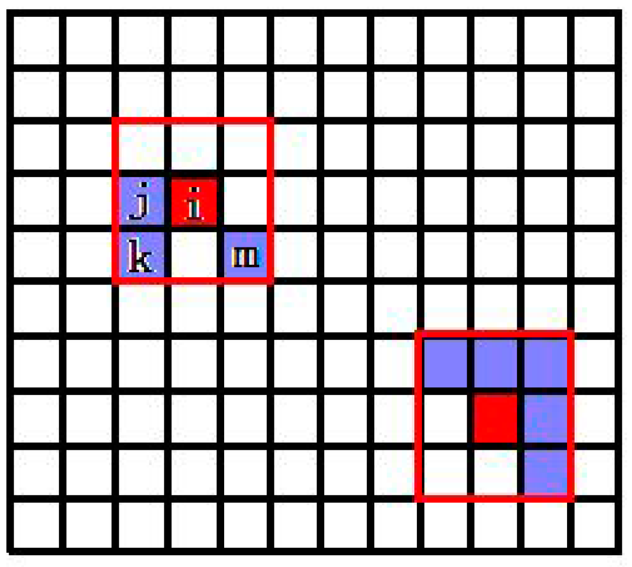
3.1. Space Consistency Constraint
- (1)
- The pixels of the near neighbourhood in the image have similar endmembers and their corresponding abundance.
- (2)
- The pixels of the near spectral distance have similar endmembers and their corresponding abundance.
- (3)
- At the same time, combined with the above two points, selecting p pixels with the nearest distance to the current pixels in the n neighbourhood as its real neighbourhood, constrain its abundances to be similar.
| Algorithm 1: Solve the SCC-LRR problem by ALM |
| Input: library A, data matrix Y, near neighbourhood consistency constraint matrix H, and regularization parameter λ, β. Initialize: X = J = L = 0, E = 0, Y1 = 0, Y2 = 0, Y3 = 0, µ = 10–6, maxu = 1010, ρ = 1.1, ε = 10–8. while not converged do 1: Fix the others and update J by , . 2: Fix the others and update X by . 3: Fix the others and update E by . 4: Fix the others and update L by . 5: Update the multipliers . 6: Update the parameter μ by . 7: check the convergence condition . end Output: representation coefficient X. |
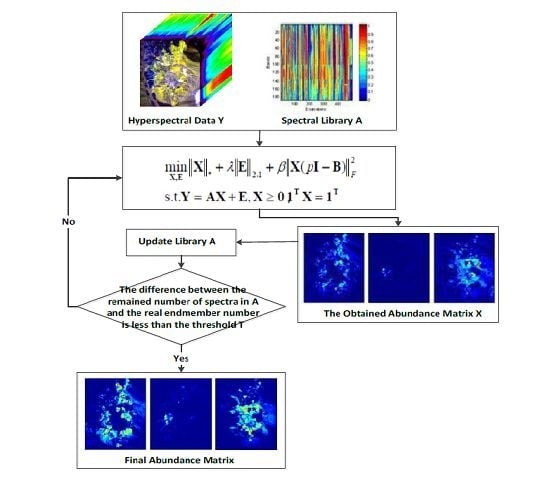
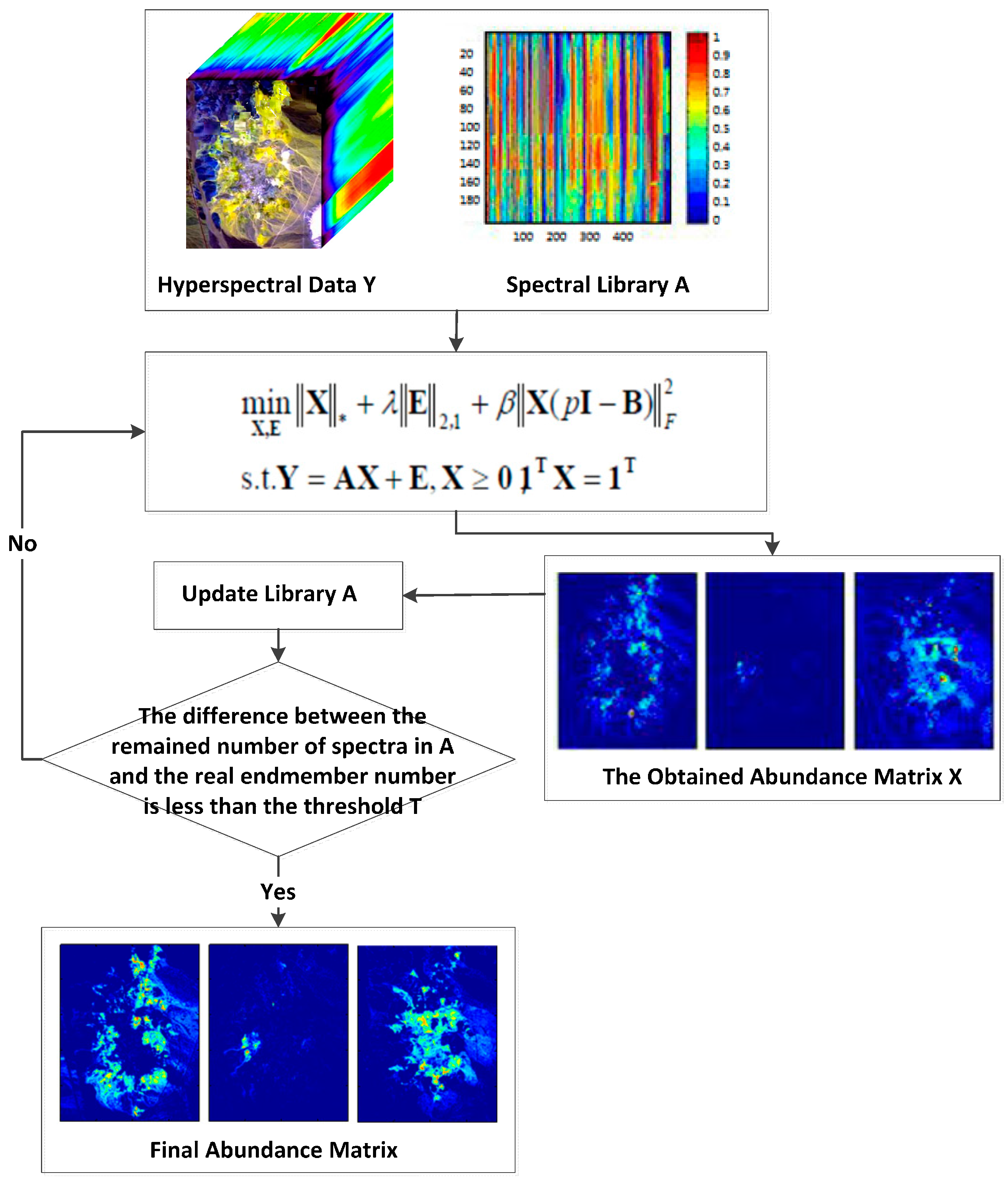
3.2. Spectral Library Pruning
- (1)
- Compute the number of the pixels whose abundance value corresponding to one endmember is smaller than a preset threshold denoted by .
- (2)
- If the number is equal to the total number of pixels in the scene, we will get rid of the spectral signature from the endmember matrix.
4. Experiments with Simulated Data and Real Data
4.1. Simulated Datasets
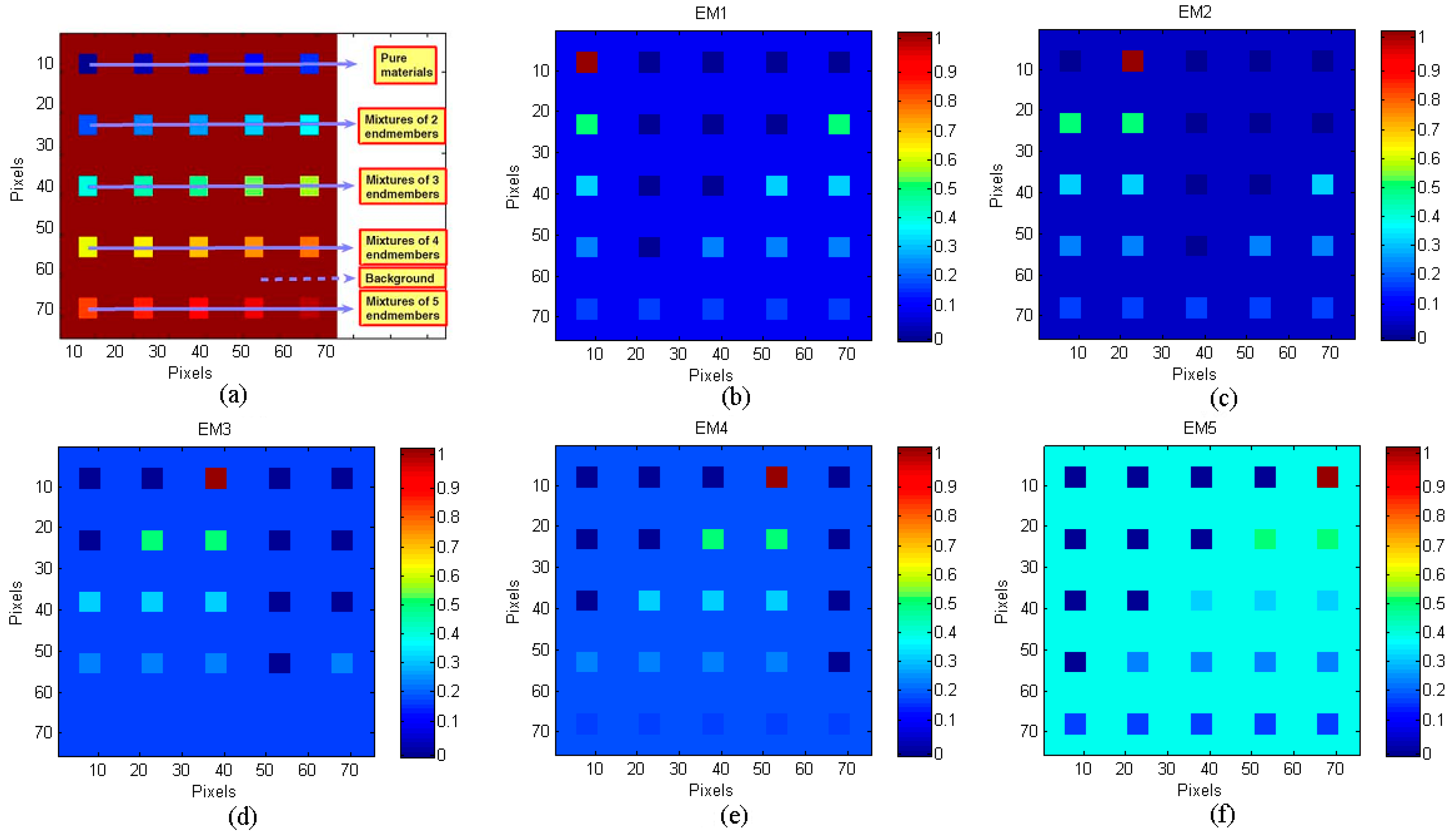
- (1)
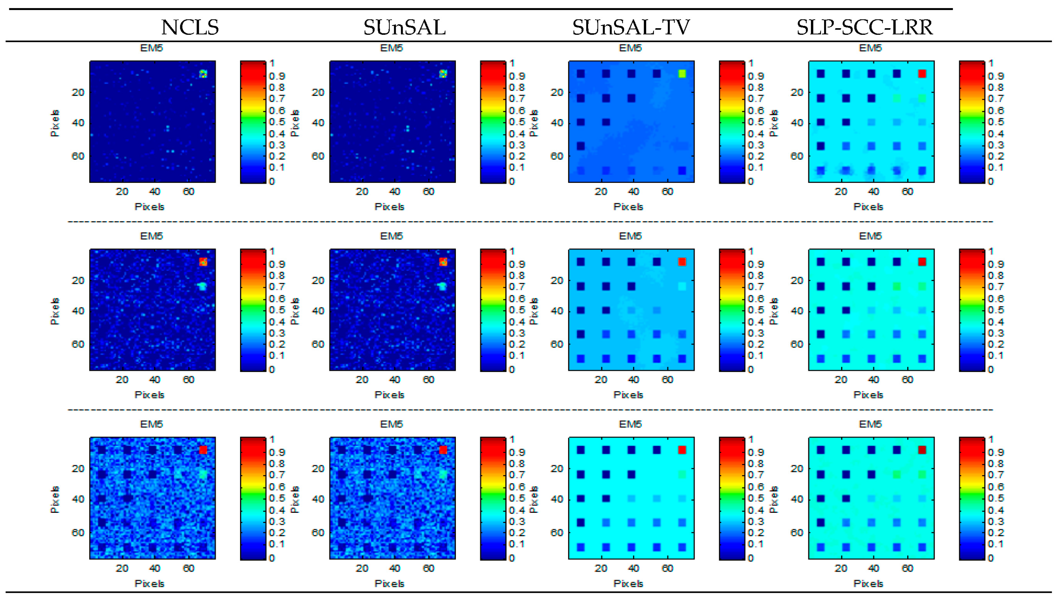
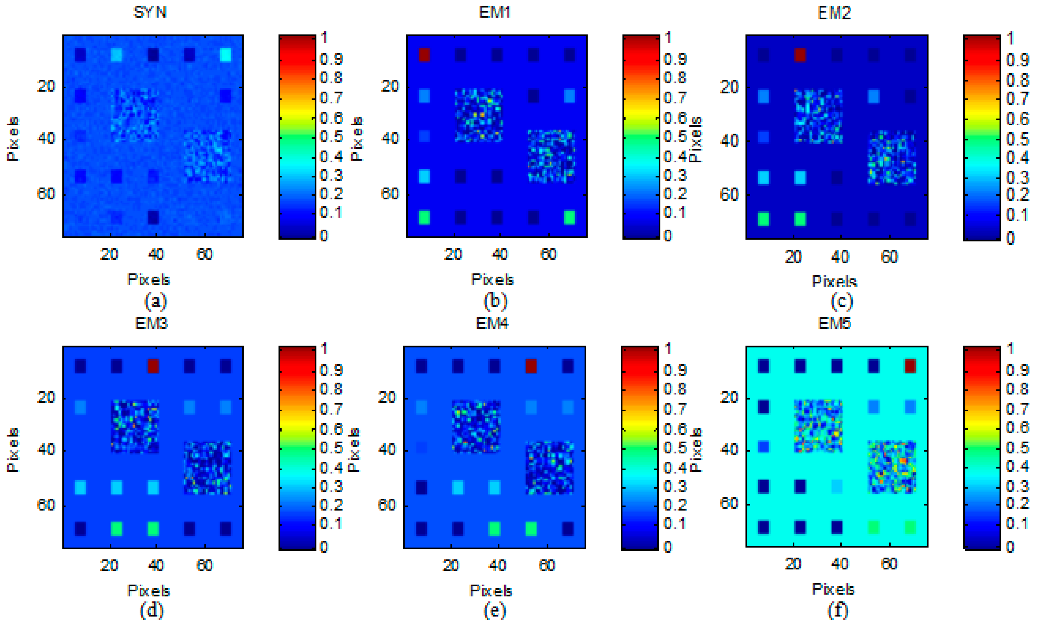
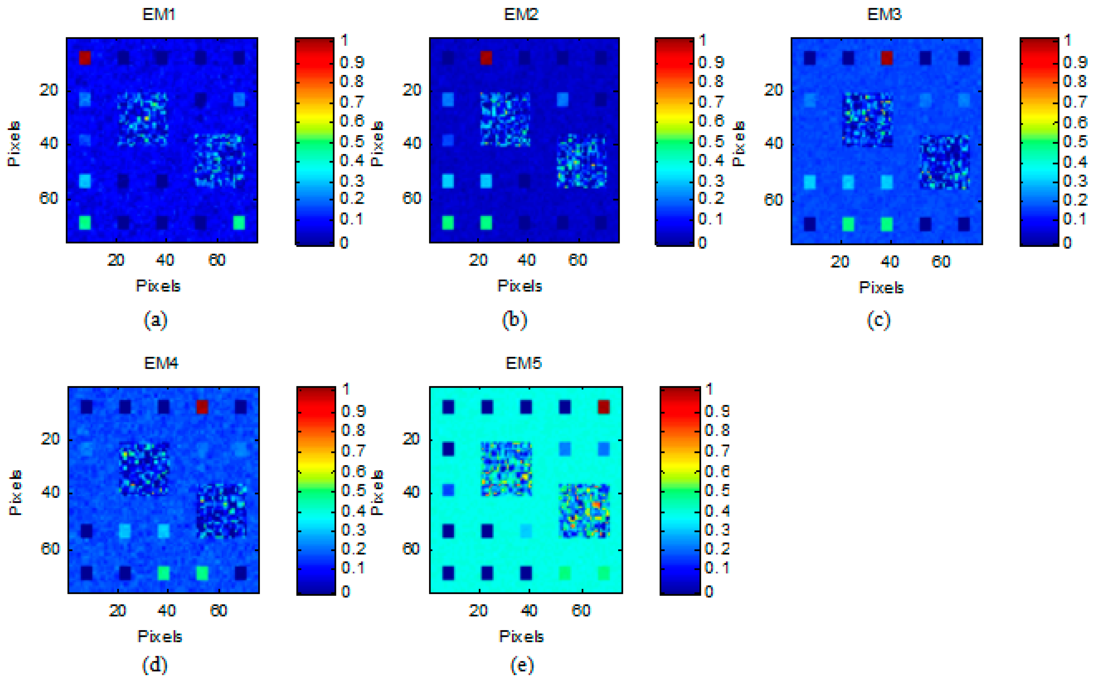
- Simulated Data Cube 1 (DC1): This simulated data cube is generated following the methodology of [26], using five randomly selected spectral signatures from A1. DC1 has 75 × 75 pixels and each simulated pixel was generated using a LMM, with the five endmembers and imposing the ASC in it. In the resulting simulated image, shown in Figure 3a, there are pure regions as well as mixed regions constructed using mixtures ranging between two and five endmembers, distributed spatially in the form of distinct square regions. Figure 3b–f, respectively, shows the true fractional abundances for each of the five endmembers. The background pixels are made up of mixtures of the same five endmembers, but their respective fractional abundances values were randomly fixed as 0.1149, 0.0741, 0.2003, 0.2055 and 0.4051, respectively. The obtained data cube was then contaminated with white noise, having different levels of the signal-to-noise ratio (SNR): 20, 30 and 40 dB.
- (2)
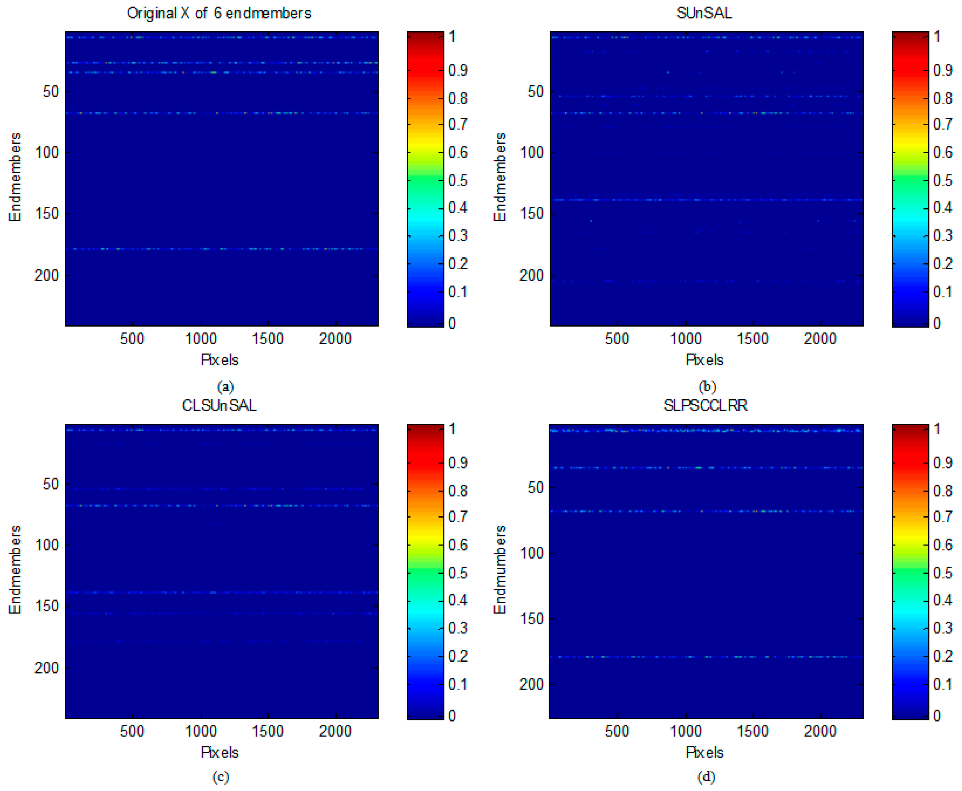
- Simulated Data Cube 2 (DC2): Using the library A1, we generated a data cube of 48 × 48 pixels and it contains six endmembers. The endmembers were randomly selected from library A1. In each simulated pixel, the fractional abundances of the endmembers follow a Dirichlet distribution [14]. As DC1, the scene was again contaminated with white noise using the same SNR value adopted for DC1.
- (3)
- Simulated Data Cube 3 (DC3): Using the library A1, we generate various data cubes of 75 × 75 pixels, each containing five endmembers. The simulated method is similar to the first simulated data. There are pure regions as well as mixed regions constructed using mixtures ranging between two and five endmembers, distributed spatially in the form of distinct square regions. The background pixels are made up of mixtures of the same five endmembers, but their respective fractional abundances values were randomly fixed as 0.1149, 0.0741, 0.2003, 0.2055 and 0.4051, respectively. The obtained data cube was then contaminated with white noise
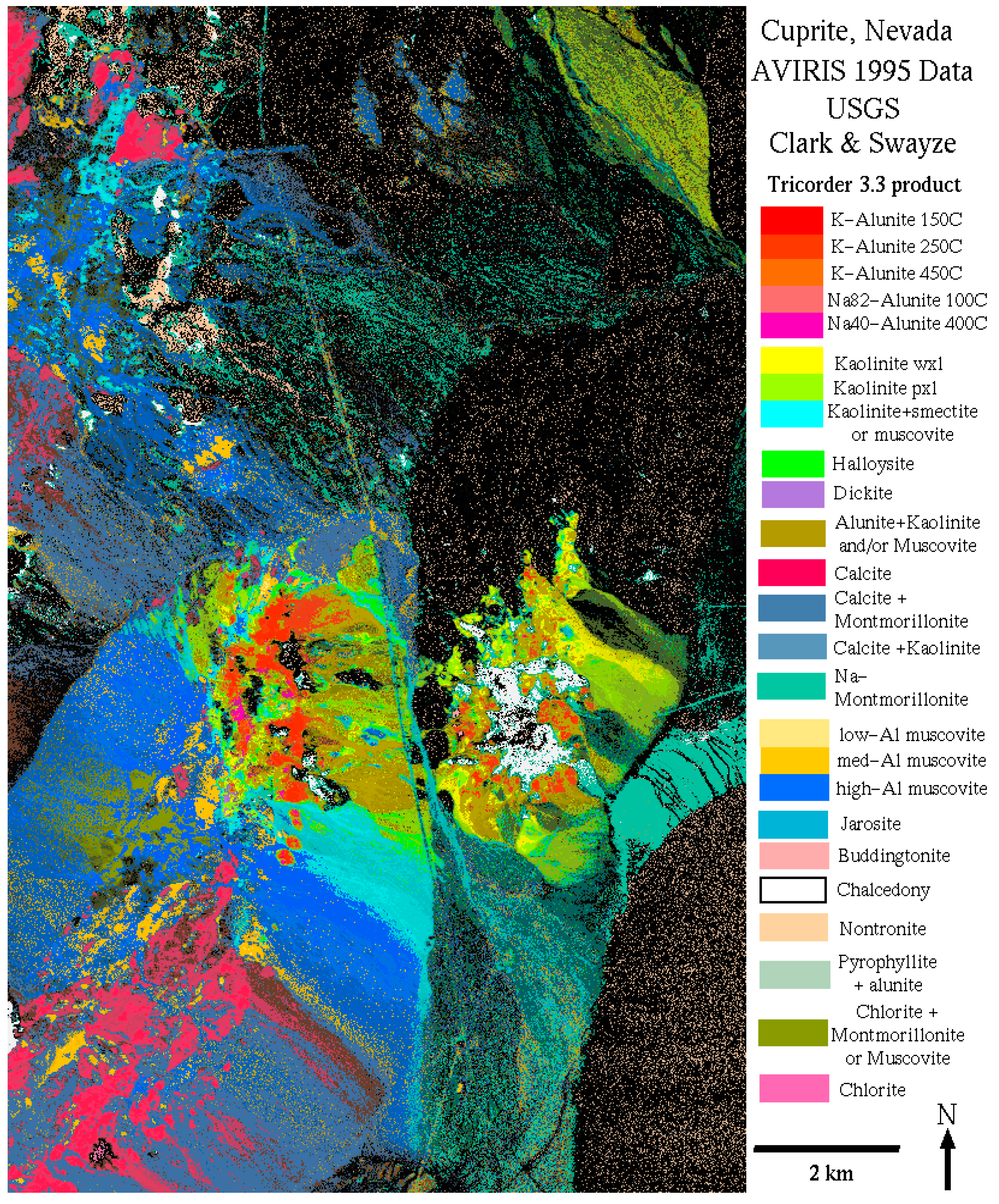
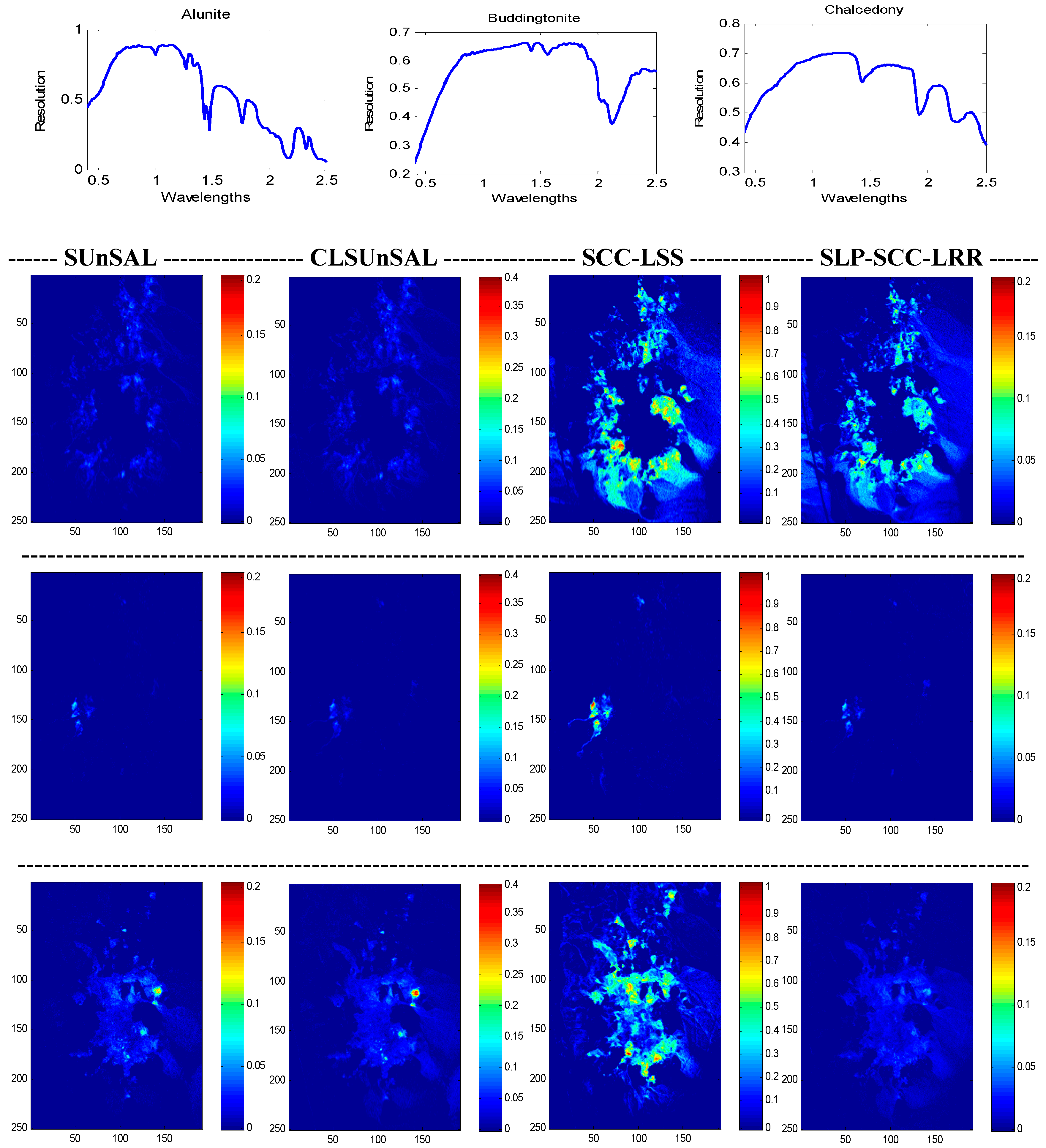
4.2. Real Datasets
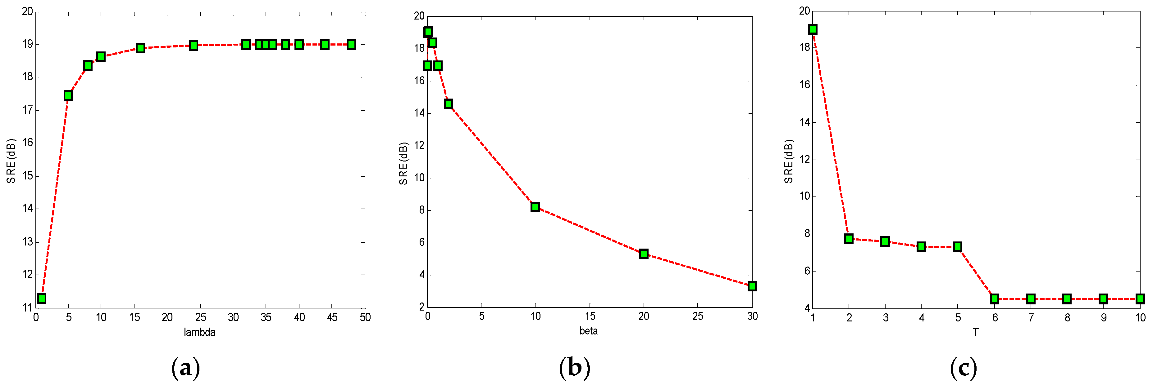
4.3. Discussion of the Parameters Setting and Time Complexity
5. Conclusions
Acknowledgments
Author Contributions
Conflicts of Interest
References
- Plaza, A.; Du, Q.; Bioucas-Dias, J. Foreword to the special issue on spectral unmixing of remotely sensed data. IEEE Trans. Geosci. Remote Sens. 2011, 49, 4103–4110. [Google Scholar] [CrossRef]
- Bioucas-Dias, J.M.; Plaza, A.; Dobigeon, N. Hyperspectral unmixing overview: Geometrical, statistical, and sparse regression-based approaches. IEEE J. Sel. Top. Appl. Earth Obs. 2012, 5, 354–379. [Google Scholar] [CrossRef]
- Keshava, N.; Mustard, J.F. Spectral unmixing. IEEE Signal Process. Mag. 2002, 19, 44–57. [Google Scholar] [CrossRef]
- Settle, J.; Drake, N. Linear mixing and the estimation of ground cover proportions. Int. J. Remote Sens. 1993, 14, 1159–1177. [Google Scholar] [CrossRef]
- Borel, C.; Gerstl, S. Nonlinear spectral mixing model for vegetative and soil surfaces. Remote Sens. Environ. 1994, 47, 403–416. [Google Scholar]
- Liu, W.; Wu, E. Comparison of non-linear mixture models. Remote Sens. Environ. 2004, 18, 1976–2003. [Google Scholar]
- Raksuntorn, N.; Du, Q. Nonlinear spectral mixture analysis for hyperspectral imagery in an unknown environment. IEEE Geosci. Remote Sens. Lett. 2010, 7, 836–840. [Google Scholar]
- Ahmed, M.; Duran, O.; Zweiri, Y. Hybrid spectral unmixing: Using artificial neural networks for linear/non-linear switching. Remote Sens. 2017, 9, 775. [Google Scholar] [CrossRef]
- Plaza, A.; Martinez, P.; Perez, R. A quantitative and comparative analysis of endmember extraction algorithms from hyperspectral data. IEEE Trans. Geosci. Remote Sens. 2004, 42, 650–663. [Google Scholar] [CrossRef]
- Du, Q.; Raksuntorn, N.; Younan, N. End-member extraction for hyperspectral image analysis. Appl. Opt. 2008, 47, 77–84. [Google Scholar] [CrossRef]
- Heinz, D.; Chang, C.-I. Fully constrained least squares linear mixture analysis for material quantification in hyperspectral imagery. IEEE Trans. Geosci. Remote Sens. 2001, 39, 529–545. [Google Scholar] [CrossRef]
- Boardman, J.W.; Kruse, F.A.; Green, R.O. Mapping target signatures via partial unmixing of AVIRIS data. In Proceedings of the Fifth JPL Airborne Earth Science Workshop, Pasadena, CA, USA, 23–26 January 1995; pp. 95–101. [Google Scholar]
- Winter, M.E. N-FINDR: An algorithm for fast autonomous spectral end-member determination in hyperspectral data. In Proceedings of the SPIE Imaging Spectrometry V, Denver, CO, USA, 19–21 July 2003; Volume 3753, pp. 266–275. [Google Scholar]
- Nascimento, J.; Bioucas-Dias, J. Vertex component analysis: A fast algorithm to unmix hyperspectral data. IEEE Trans. Geosci. Remote Sens. 2005, 43, 898–910. [Google Scholar] [CrossRef]
- Neville, R.A.; Staenz, K.; Szeredi, T.; Lefebvre, J. Automatic endmember extraction from hyperspectral data for mineral exploration. In Proceedings of the 21st Canadian Symposium on remote Sensing, Ottawa, ON, Canada, 21–24 July 1999; pp. 891–897. [Google Scholar]
- Berman, M.; Kiiveri, H.; Lagerstrom, R. ICE: A statistical approach to identifying endmembers in hyperspectral images. IEEE Trans. Geosci. Remote Sens. 2004, 42, 2085–2095. [Google Scholar] [CrossRef]
- Iordache, M.D.; Bioucas-Dias, J.M.; Plaza, A. Sparse unmixing of hyperspectral data. IEEE Trans. Geosci. Remote Sens. 2011, 49, 2014–2039. [Google Scholar] [CrossRef]
- Li, J.; Dias, J.M.B.; Plaza, A. Robust collaborative nonnegative matrix factorization for hyperspectral unmixing. IEEE Trans. Geosci. Remote Sens. 2016, 54, 6076–6090. [Google Scholar] [CrossRef]
- Bioucas-Dias, J.; Figueiredo, M. Alternating direction algorithms for constrained sparse regression: Application to hyperspectral unmixing. In Proceedings of the 2010 2nd Workshop on Hyperspectral Image and Signal Processing: Evolution in Remote Sensing (WHISPERS), Reykjavik, Iceland, 14–16 June 2010; pp. 1–4. [Google Scholar]
- Donoho, D.; Elad, M. Optimal sparse representation in general (nonorthogonal) dictionaries via l1 minimization. Proc. Natl. Acad. Sci. USA 2003, 100, 2197–2202. [Google Scholar] [CrossRef] [PubMed]
- Van der Meer, F.D.; Jia, X. Collinearity and orthogonality of endmembers in linear spectral unmixing. Int. J. Appl. Earth Obs. Geoinf. 2012, 18, 491–503. [Google Scholar] [CrossRef]
- Chen, X.; Chen, J.; Jia, X. A quantitative analysis of virtual endmembers’ increased impact on the collinearity effect in spectral unmixing. IEEE Trans. Geosci. Remote Sens. 2011, 49, 2945–2956. [Google Scholar] [CrossRef]
- Iordache, M.D.; Bioucas-Dias, J.M.; Plaza, A. Total variation spatial regularization for sparse hyperspectral unmixing. IEEE Trans. Geosci. Remote Sens. 2012, 50, 4484–4502. [Google Scholar] [CrossRef]
- Iordache, M.D.; Bioucas-Dias, J.M.; Plaza, A. Hyperspectral unmixing with sparse group lasso. In Proceedings of the 2011 IEEE International Geoscience and Remote Sensing Symposium (IGARSS), Vancouver, BC, Canada, 24–29 July 2011; pp. 3586–3589. [Google Scholar]
- Sprechmann, P.; Ramirez, I.; Sapiro, G.; Eldar, Y. C-Hilasso: A collaborative hierarchical sparse modeling framework. IEEE Trans. Signal Process. 2011, 59, 4183–4198. [Google Scholar] [CrossRef]
- Iordache, D.; Bioucas-Dias, J.; Plaza, A. Collaborative sparse regression for hyperspectral unmixing. IEEE Trans. Geosci. Remote Sens. 2014, 52, 341–354. [Google Scholar] [CrossRef]
- Li, C.; Ma, Y. Sparse unmixing of hyperspectral data with noise level estimation. Remote Sens. 2017, 9, 1166. [Google Scholar] [CrossRef]
- Zhang, Y.; Jiang, Z.; Davis, L.S. Learning structured low-rank representations for image classification. In Proceedings of the IEEE Conference on Computer Vision and Pattern Recognition, Portland, OR, USA, 23–28 June 2013. [Google Scholar]
- Williams, M.D.; Parody, R.J. Validation of abundance map reference data for spectral unmixing. Remote Sens. 2017, 9, 473. [Google Scholar] [CrossRef]
- Qian, Y.; Xiong, F. Matrix-vector nonnegative tensor factorization for blind unmixing of hyperspectral imagery. IEEE Trans. Geosci. Remote Sens. 2017, 55, 1776–1792. [Google Scholar] [CrossRef]
- Fan, H.; Chen, Y. Hyperspectral image restoration using low-rank tensor recovery. IEEE J. Sel. Top. Appl. Earth Obs. Remote Sens. 2017, 10, 4589–4604. [Google Scholar] [CrossRef]
- Ertürk, A.; Iordache, M.-D.; Plaza, A. Sparse unmixing based change detection for multitemporal hyperspectral images. IEEE J. Sel. Top. Appl. Earth Obs. Remote Sens. 2016, 9, 708–719. [Google Scholar] [CrossRef]
- Ertürk, A.; Iordache, M.-D.; Plaza, A. Sparse unmixing with dictionary pruning for hyperspectral change detection. IEEE J. Sel. Top. Appl. Earth Obs. Remote Sens. 2017, 10, 321–330. [Google Scholar] [CrossRef]
- Zortea, M.; Plaza, A. Spatial preprocessing for endmember extraction. IEEE Trans. Geosci. Remote Sens. 2009, 47, 2679–2693. [Google Scholar] [CrossRef]
- Plaza, A.; Martinez, P.; Perez, R. Spatial/spectral endmember extraction by multidimensional morphological operations. IEEE Trans. Geosci. Remote Sens. 2002, 40, 2025–2041. [Google Scholar] [CrossRef]
- Rogge, D.; Rivard, B.; Zhang, J. Integration of spatial-spectral information for the improved extraction of endmembers. Remote Sens. Environ. 2007, 110, 287–303. [Google Scholar] [CrossRef]
- Horn, R.; Johnson, C. Matrix Analysis; Cambridge University Press: Cambridge, UK, 1990. [Google Scholar]
- Qu, Q.; Nasrabadi, N.M.; Tran, T.D. Abundance estimation for bilinear mixture models via joint sparse and low-rank representation. IEEE Trans. Geosci. Remote Sens. 2014, 52, 4404–4423. [Google Scholar]
- Liu, G.; Lin, Z.; Yan, S. Robust recovery of subspace structures by low-rank representation. IEEE Trans. Pattern Anal. Mach. Intell. 2013, 35, 171–184. [Google Scholar] [CrossRef] [PubMed]
- Liu, G.; Lin, Z.; Yu, Y. Robust subspace segmentation by low rank representation. In Proceedings of the 27th International Conference on International Conference on Machine Learning, Haifa, Israel, 21–24 June 2010; pp. 663–670. [Google Scholar]
- Zhouchen, L.; Minming, C.; Leqin, W. The Augmented Lagrange Multiplier Method for Exact Recovery of Corrupted Low-Rank Matrices; Technical Report, UIUC Technical Report UILU-ENG-09-2215; University of Illinois at Urbana–Champaign (UIUC): Champaign, IL, USA, 2009. [Google Scholar]
- Fazel, M. Matrix Rank Minimization with Applications. Ph.D. Thesis, Department of Electrical Engineering, Stanford University, Stanford, CA, USA, 2002. [Google Scholar]
- Iordache, M.-D.; Bioucas-Dias, J.M.; Plaza, A. MusicCSR: Hyperspectral unmixing via multiple signal classification and collaborative sparse regression. IEEE Trans. Geosci. Remote Sens. 2014, 52, 4364–4382. [Google Scholar] [CrossRef]
- Shi, Z.; Tang, W.; Duren, Z. Subspace matching pursuit for sparse unmixing of hyperspectral data. IEEE Trans. Geosci. Remote Sens. 2013, 52, 3256–3274. [Google Scholar] [CrossRef]


| Methods | DC1 | SNR = 20 dB | SNR = 30 dB | SNR = 40 dB |
|---|---|---|---|---|
| NCLS | SRE | 1.2648 | 2.5000 | 7.5332 |
| AAD | 0.8512 | 0.5657 | 0.2211 | |
| SUnSAL | SRE | 1.5753 | 3.2432 | 8.2820 |
| AAD | 0.8276 | 0.6414 | 0.1853 | |
| SUnSAL-TV | SRE | 5.5956 | 15.0211 | 23.6639 |
| AAD | 0.4530 | 0.0486 | 0.0206 | |
| LRR | SRE | 1.6232 | 3.5426 | 6.7140 |
| AAD | 0.4777 | 0.2779 | 0.1401 | |
| SCC-LRR | SRE | 2.8598 | 5.1026 | 4.8676 |
| AAD | 0.1838 | 0.0753 | 0.1823 | |
| SLP-SCC-LRR | SRE | 21.8418 | 32.7520 | 44.5256 |
| AAD | 0.0318 | 0.0221 | 0.0074 |
| Methods | DC1 | SNR = 20 dB | SNR = 30 dB | SNR = 40 dB |
|---|---|---|---|---|
| NCLS | Times | 41.8314 | 28.7967 | 23.2396 |
| SUnSAL | Parameters | λ = 8 × 10⁻² | λ = 8 × 10⁻² | λ = 1 × 10⁻² |
| Times | 21.2719 | 22.4660 | 24.2318 | |
| SUnSAL-TV | Parameters | λ = 5 × 10⁻² λTV = 5 × 10⁻² | λ = 5 × 10⁻³ λTV = 1 × 10⁻² | λ = 3 × 10⁻³ λTV = 5 × 10⁻³ |
| Times | 523.0716 | 527.0992 | 611.4388 | |
| LRR | Parameters | λ = 0.5 | λ = 4 | λ = 70 |
| Times | 861.1286 | 936.9994 | 784.9693 | |
| SCC-LRR | Parameters | λ = 6 β = 100 | λ =15 β = 110 | λ = 6 β = 100 |
| Times | 232.0626 | 246.2892 | 264.2972 | |
| SLP-SCC-LRR | Parameters | λ = 6 β = 100 T = 3 | λ = 15 β = 110 T = 2 | λ = 6 β = 100 T = 1 |
| Times | 400.3627 | 374.6602 | 412.6240 |
| Methods (DC2) | SNR = 20 dB | SNR = 30 dB | SNR = 40 dB | |||
|---|---|---|---|---|---|---|
| SRE | AAD | SRE | AAD | SRE | AAD | |
| SUnSAL | 1.7227 | 0.9619 | 3.1024 | 0.7060 | 6.0602 | 0.3963 |
| CLSUnSAL | 2.1666 | 0.7251 | 4.0155 | 0.4013 | 9.4707 | 0.0958 |
| LRR | 1.7299 | 0.5822 | 3.0060 | 0.3143 | 4.0263 | 0.1781 |
| SCC-LRR | 0.6004 | 0.4881 | 1.3476 | 0.2931 | 1.7065 | 0.2102 |
| SMP + SUnSAL | 2.1126 | 0.8923 | 3.4765 | 0.6654 | 6.9170 | 0.3579 |
| SMP + CLSUnSAL | 2.9256 | 0.8083 | 4.3575 | 0.2092 | 7.6023 | 0.2367 |
| SMP + LRR | 1.8926 | 0.5424 | 3.0206 | 0.3123 | 4.7494 | 0.1866 |
| SMP + SCC-LRR | 0.6582 | 0.4881 | 1.4118 | 0.2931 | 1.7759 | 0.2102 |
| RSFoBa + SUnSAL | 2.3032 | 0.8520 | 5.4326 | 0.4982 | 11.5092 | 0.2134 |
| RSFoBa + CLSUnSAL | 2.8469 | 0.6162 | 9.6058 | 0.1628 | 20.3783 | 0.0521 |
| RSFoBa + LRR | 2.5989 | 0.4672 | 5.4969 | 0.3503 | 9.8677 | 0.1443 |
| RSFoBa + SCC-LRR | 0.7044 | 0.4881 | 1.6437 | 0.2931 | 1.9177 | 0.2102 |
| SLP + SUnSAL | 4.9159 | 0.5632 | 18.9343 | 0.1100 | 28.5571 | 0.0363 |
| SLP + CLSUnSAL | 3.6273 | 0.3010 | 19.0567 | 0.1090 | 28.4343 | 0.0367 |
| SLP-LRR | 5.3920 | 0.3386 | 19.0560 | 0.1090 | 28.5731 | 0.0363 |
| SLP-SCC-LRR | 4.4974 | 0.4054 | 19.0002 | 0.1097 | 28.4715 | 0.0366 |
| Methods (DC2) | SNR = 20 dB | SNR = 30 dB | SNR = 40 dB | |||
|---|---|---|---|---|---|---|
| Parameters | Times | Parameters | Times | Parameters | Times | |
| SUnSAL | λ = 0.05 | 16.9724 | λ = 0.01 | 11.6911 | λ = 1 × 10⁻³ | 8.7732 |
| CLSUnSAL | λ = 0.9 | 40.8787 | λ = 0.2 | 41.5278 | λ = 0.05 | 41.3956 |
| LRR | λ = 2 | 206.4049 | λ = 20 | 182.7591 | λ = 50 | 164.0270 |
| SCC-LRR | λ = 2 β = 0.01 | 122.5415 | λ = 36 β = 0.1 | 109.7295 | λ = 6 β = 0.01 | 117.2215 |
| SMP + SUnSAL | λ = 0.08 | 6.4694 | λ = 0.01 | 6.1948 | λ = 9 × 10⁻⁴ | 4.6662 |
| SMP + CLSUnSAL | λ = 2 | 11.8081 | λ = 0.2 | 12.5174 | λ = 8 × 10⁻³ | 12.5302 |
| SMP + LRR | λ = 2 | 64.0299 | λ = 10 | 73.1744 | λ = 80 | 79.6736 |
| SMP + SCC-LRR | λ =2 β = 0.01 | 114.3858 | λ =36 β = 0.1 | 111.7261 | λ = 6 β = 0.01 | 123.7080 |
| RSFoBa + SUnSAL | λ = 0.03 | 3.1553 | λ = 4 × 10⁻³ | 1.9873 | λ = 6 × 10⁻⁴ | 0.8679 |
| RSFoBa + CLSUnSAL | λ = 0.2 | 19.9172 | λ = 0.2 | 9.6373 | λ = 0.1 | 6.0128 |
| RSFoBa + LRR | λ = 2 | 54.3540 | λ = 35 | 35.4342 | λ = 80 | 21.1428 |
| RSFoBa + SCC-LRR | λ = 2 β = 0.01 | 118.9212 | λ = 36 β = 0.1 | 118.7259 | λ = 6 β = 0.01 | 128.7818 |
| SLP + SUnSAL | λ = 0.05 T = 10 | 76.3745 | λ = 6 × 10⁻³ T = 1 | 45.0329 | λ = 1 × 10⁻³ T = 1 | 19.0163 |
| SLP + CLSUnSAL | λ = 2 T = 10 | 25.0145 | λ = 0.1 T = 1 | 33.0251 | λ = 0.04 T = 1 | 23.7061 |
| SLP-LRR | λ = 2 T = 10 | 689.9156 | λ = 8 T = 1 | 471.5313 | λ = 80 T = 1 | 324.2536 |
| SLP-SCC-LRR | λ = 2 β = 0.01 T = 10 | 290.9236 | λ = 36 β = 0.1 T = 1 | 489.6472 | λ = 6 β = 0.01 T = 1 | 323.6368 |
| Methods | DC3 | SNR = 40 dB | Parameters | Times |
|---|---|---|---|---|
| LRR | SRE | 0.2997 | λ = 1 × 10⁻¹ | 486.9841 |
| AAD | 1.1210 | |||
| SUnSAL | SRE | 0.2419 | λ = 1 × 10⁻² | 11.4843 |
| AAD | 1.2584 | |||
| SUnSAL-TV | SRE | 0.0971 | λ = 1 λTV = 5 × 10⁻² | 228.4922 |
| AAD | 0.9397 | |||
| SCC-LRR | SRE | 0.4061 | λ = 10 β = 50 | 232.9945 |
| AAD | 0.8596 | |||
| SLP-SCC-LRR | SRE | 22.3349 | λ = 1 β = 111 T = 1 | 840.1768 |
| AAD | 0.0903 |
© 2018 by the authors. Licensee MDPI, Basel, Switzerland. This article is an open access article distributed under the terms and conditions of the Creative Commons Attribution (CC BY) license (http://creativecommons.org/licenses/by/4.0/).
Share and Cite
Zhang, X.; Li, C.; Zhang, J.; Chen, Q.; Feng, J.; Jiao, L.; Zhou, H. Hyperspectral Unmixing via Low-Rank Representation with Space Consistency Constraint and Spectral Library Pruning. Remote Sens. 2018, 10, 339. https://doi.org/10.3390/rs10020339
Zhang X, Li C, Zhang J, Chen Q, Feng J, Jiao L, Zhou H. Hyperspectral Unmixing via Low-Rank Representation with Space Consistency Constraint and Spectral Library Pruning. Remote Sensing. 2018; 10(2):339. https://doi.org/10.3390/rs10020339
Chicago/Turabian StyleZhang, Xiangrong, Chen Li, Jingyan Zhang, Qimeng Chen, Jie Feng, Licheng Jiao, and Huiyu Zhou. 2018. "Hyperspectral Unmixing via Low-Rank Representation with Space Consistency Constraint and Spectral Library Pruning" Remote Sensing 10, no. 2: 339. https://doi.org/10.3390/rs10020339