A Hierarchical Fully Convolutional Network Integrated with Sparse and Low-Rank Subspace Representations for PolSAR Imagery Classification


1
Electronic Information School, Wuhan University, Wuhan 430072, China
2
State Key Laboratory for Information Engineering in Surveying, Mapping and Remote Sensing, Wuhan University, Wuhan 430079, China
3
Collaborative Innovation Center of Geospatial Technology, 129 Luoyu Road, Wuhan 430079, China
*
Author to whom correspondence should be addressed.
Remote Sens. 2018, 10(2), 342; https://doi.org/10.3390/rs10020342
Submission received: 14 January 2018
/
Revised: 10 February 2018
/
Accepted: 13 February 2018
/
Published: 23 February 2018
(This article belongs to the Special Issue Deep Learning for Remote Sensing)
Abstract
:Inspired by enormous success of fully convolutional network (FCN) in semantic segmentation, as well as the similarity between semantic segmentation and pixel-by-pixel polarimetric synthetic aperture radar (PolSAR) image classification, exploring how to effectively combine the unique polarimetric properties with FCN is a promising attempt at PolSAR image classification. Moreover, recent research shows that sparse and low-rank representations can convey valuable information for classification purposes. Therefore, this paper presents an effective PolSAR image classification scheme, which integrates deep spatial patterns learned automatically by FCN with sparse and low-rank subspace features: (1) a shallow subspace learning based on sparse and low-rank graph embedding is firstly introduced to capture the local and global structures of high-dimensional polarimetric data; (2) a pre-trained deep FCN-8s model is transferred to extract the nonlinear deep multi-scale spatial information of PolSAR image; and (3) the shallow sparse and low-rank subspace features are integrated to boost the discrimination of deep spatial features. Then, the integrated hierarchical subspace features are used for subsequent classification combined with a discriminative model. Extensive experiments on three pieces of real PolSAR data indicate that the proposed method can achieve competitive performance, particularly in the case where the available training samples are limited.
1. Introduction
1.1. Background
Synthetic Aperture Radar (SAR), characterized by almost all-weather, all-day imaging capability, has become increasingly important in various Earth observation applications. As an advanced type of SAR, the fully polarimetric SAR (PolSAR) measures the complex scattering matrix of a medium with quad polarizations, which contains the amplitude, phase and polarimetric characteristics of targets. Thus, PolSAR data can greatly improve the ability to identify different terrain targets when used for classification tasks. Recently, extensive attention to this topic has gradually arisen.
Over the past few decades, numerous pixel-based classification methods have been proposed, which generally employ one of three major types of information [1]: (1) the statistical characteristics of the scattering coherent matrix [2,3]; (2) the inherent characteristics of polarimetric scattering mechanisms [4,5]; and (3) the combination of statistical properties and polarimetric scattering characteristics [6,7,8]. However, under the influence of speckle noise, the features based on pixel-wise polarimetric target decomposition parameters cannot perform well. To solve the problem, semantic information such as spatial relations, texture, shape, etc. should be concerned, hence an mount of region-based methods have been developed. A common way is to use the Markov random field and conditional random field to model the spatial interactions [9,10,11], or segment data into homogeneous objects [12]. In addition, some researchers also undertake to combine the neural network models with superpixel segmentation to remedy this matter [13,14].
Although the region-based approaches can obviously improve classification results, they are shallow in architectures, thus can extract only low-level handcrafted spatial features of the original data, whose representation and discrimination abilities are usually limited. Especially for PolSAR data with high spatial resolution, most shallow methods will fail. Thus, one needs an in-depth understanding of the involved physics with a deep model, as well as to automatically learn high-level spatial representations from PolSAR data.
SAR Image Classification Meets Deep Learning. Recently, deep learning (DL), a powerful technique for adaptively learning the representative and discriminative features in a hierarchical manner from data, has become a hot topic in remote sensing community. So far, the DL-related studies for SAR image classification can be roughly divided into two large categories [15]. The first category involves the unsupervised generative graphical models, such as autoencoder neural networks, the deep belief networks (DBN) and restricted Boltzmann machines (RBM). Xie et al. [16] introduce stacked sparse autoencoder (SAE), constructed by multiple SAEs, to learn features automatically instead of the handcrafted feature for PolSAR image classification. To reduce speckle noise, researchers in [17] improve the SAE method to deep convolutional autoencoder by adding a convolutional layer and a scale transformation layer. In addition, to obtain effective feature representation when denoising, Geng et al. [18] propose a novel deep supervised and contractive neural network that consists of four layers of supervised and contractive autoencoders. Lv et al. [19] carry out the DBN model on urban land use and land cover classification, which can extract contextual mapping features with preserved shape details. However, the DBN model cascaded by multiple RBMs requires large data volumes. To address this problem, authors in [12] use RBM as the base classifier to construct an ensemble boosting model to perform object-oriented classification.
The other stream of the DL-related SAR image classification studies is based on the supervised convolutional neural network (CNN). Zhou et al. [20] employ a four-layer CNN to perform PolSAR image classification on six-channel real-valued data. Following this idea, Zhang et al. [21] propose a complex-valued CNN (CV-CNN), which extends the entire network into the complex domain, to fully utilize amplitude and phase information of complex SAR imagery. However, the patch-based CNN can just predict one label for the entire image. To overcome the drawback, Wang et al. [22] integrate H-A- polarimetric decomposition with a fully convolutional network (FCN) [23], which is fine-tuned based on a deep VGG-16 CNN, to obtain an end-to-end PolSAR image classification.
So far, the research on DL for remote sensing data analysis is still young and many problems remain to be solved. In summary, there exist four major challenges [24]: (1) the lack of high-quality training samples; (2) the complexity of remote sensing data prevents learning robust and discriminative representations; (3) the transfer problem between data sets from different sensors; and (4) the selection of the proper depth of a DL model when the computation time and training data are limited. As a result, it is not practical to completely rely on deep learning to cope with the PolSAR classification task at present. In this case, a synergy of physics-based model and DL model will be a promising direction [15], which is the main standing point of this study.
Sparse and Low-Rank Representations. Recently, a growing number of publications show that sparse and low-rank representations can convey valuable information for image processing and pattern classification. From the point of statistical signal processing, sparse representation (SR) is based on an over-complete dictionary consisting of basic vectors, and it represents the input signal as the sparsest linear combination of basic vectors [25]. The great potential of SR to interpret remote sensing images has been explored. Authors in [26] present an SAR target classification approach that uses SR to describe the local features in each sub-region. Zhang et al. [27] propose an SR-based supervised classification method for PolSAR image. Fang et al. [28] perform multiclasses classification for large area glacier based on two layers of sparse learning. These methods fully take advantage of the local discrimination of sparse representations of features. However, SR seeks the sparsest representation of each sample individually, lacking global constraints on its solutions; thus, the SR-based methods may be ineffective in capturing the global structure of data.
Different from SR, low-rank representation (LRR) proposed first in [29] aims at seeking the lowest-rank representation of a group of vectors jointly, and thus can capture the global information, which has been verified useful for SAR image classification in several pioneering studies. Ren et al. [30] use LRR to capture the intrinsic global structure of PolSAR data and achieve a better classification performance. To make features more discriminative, SR and LRR should be employed jointly to make their respective advantages complementary to each other. Researchers in [31,32] combine SR with LRR to obtain the local and global structures of data simultaneously, which noticeably improve classification accuracy.
1.2. Problems and Motivation
In practice, on the one hand, for the sake of describing variety of terrain targets in study scenes as certainly as possible, a reasonable way is to bring multiple features derived from different polarimetric decomposition methods together, due to the fact that different decomposition methods can only benefit for specific types of targets. However, this kind of stacked polarimetric feature possesses high dimensionality and redundancy. Thus, an effective and efficient dimensionality reduction (DR) method is needed to capture the intrinsic structures in a low-dimensional subspace and to discard redundancy. In consideration of the important role of sparse and low-rank representations in classification tasks as discussed above, we introduce a linear DR approach, sparse and low-rank graph-based discriminant analysis (SLGDA) [31], to tackle this problem, which can capture the local and global structures of PolSAR data simultaneously.
On the other hand, motivated by enormous success of FCN in semantic segmentation [23], as well as the similarity between semantic segmentation in computer vision and pixel-wise PolSAR image classification, i.e., assigning a label for each pixel, employing FCN for the latter is possible. However, there is a little research in this area. At present, using FCN directly to perform PolSAR image classification is impractical because very few labeled PolSAR samples are available, which makes it impossible to train an effective FCN model with limited PolSAR data from scratch. Moreover, fine-tuning a pre-trained FCN model with available PolSAR data to obtain satisfied performance is also difficult without post-precessing [33], due to the imaging mechanisms of optical image and PolSAR image are inherently different, which may lead to that most of model parameters pre-trained on optical images do not hold any longer, thus the unique and critical polarimetric information of PolSAR data is not well preserved. However, it should be noted that FCN has a powerful potential to learn the nonlinear deep spatial representations. Although pre-trained on optical images, this potential is also effective for other types of images, which has been empirically verified [33,34].
It is known that land covers are continuous in the spatial domain, and adjacent pixels in a PolSAR image belong to the same class with a very high probability. Thus, the use of spatial features can significantly improve the classification accuracy, as indicated in many studies [1,11]. However, the previous methods cannot extract robust deep spatial feature representations due to their shallow architectures. Therefore, in this work, we take a pre-trained FCN model as a spatial feature extractor to exploit the nonlinear deep spatial patterns. Considering that very deep FCN is weak in capturing the local details, and from the point of view of DL, SLGDA is a shallow subspace learning and lack of spatial constraints, we integrate deep spatial features of FCN with sparse and low-rank subspace features of SLGDA to make their advantages beneficial for each other.
1.3. Contributions and Structure
This paper presents a hierarchical fully convolutional network, which is integrated with sparse and low-rank subspace representations, for PolSAR imagery classification, as shown in Figure 1. The contributions of this work are summarized as follows:
- An effective linear subspace learning based on sparse and low-rank graph embedding discriminant analysis is firstly introduced to perform DR on the stacked multiple polarimetric features, which not only removes the redundant features that potentially aggravate classification performance, but also captures the local and global structures of PolSAR data simultaneously.
- An FCN-8s model pre-trained on optical images is firstly transferred to learn the nonlinear deep multi-scale spatial features of PolSAR image, where we take Pauli-decomposed pseudo-color image as an input “RGB“ image to match model parameters. This kind of high-level semantic information learned adaptively by FCN-8s can significantly facilitate classification.
- The shallow sparse and low-rank representations of PolSAR data in a reduced-dimensional subspace are integrated with the deep spatial features by using a weighted strategy to make their advantages beneficial for each other. In the integrated hierarchical subspace features, multiple types of information, ranging from shallow to deep, linear to nonlinear, local to global, and polarimetric to spatial, is incorporated to boost the discrimination of features for subsequent classification.
The remainder of this paper is organized as follows. Section 2 introduces preliminaries about PolSAR data, subspace learning based on graph embedding and FCN architectures. The subsequent Section 3 formulates the algorithm theory of learning sparse and low-rank subspace features by SLGDA, the process of extracting multi-scale spatial features via FCN-8s and integrating hierarchical subspace features for PolSAR image classification. Section 4 presents the experimental results and analysis. Finally, the discussion and conclusion are given in Section 5 and Section 6, respectively.
2. Preliminaries
2.1. Multidimensional PolSAR Data
Polarimetric SAR focuses on emitting and receiving fully polarized radar waves to characterize terrain targets. For reciprocal media case, the responses of polarimetric SAR can be considered as the interactions of three correlated coherent interference processes: horizontal transmitting and horizontal receiving (HH), horizontal transmitting and vertical receiving (HV), as well as vertical transmitting and vertical receiving (VV) polarization channels [35]. Polarimetric radar measures the complex scattering matrix of a medium with quad polarizations. In the linear polarization base, the scattering matrix can be expressed as
where element denotes complex scattering characteristics (coefficients or amplitudes) obtained by emitting j-polarization and receiving i-polarization radar waves, respectively. In the case of monostatic backscattering in a reciprocal medium, i.e., , the polarimtric scattering information can be represented by a Pauli scattering vector, that is
where superscript T denotes the transpose operation.
Although the scattering matrix can well describe coherence or pure scatterers, most of the complex targets in the natural scene belong to the distributed scatterer, which cannot be represented by . Moreover, under the influence of speckle noise, it has to resort to a statistic method such as coherence matrix or covariance matrix to describe scattering characteristics. Based on Pauli basis, the coherence matrix generated by multilook processing is expressed as
where n and H denote the number of looks and conjugation transpose operation, respectively, and represents the ensemble average in the data processing.
Taking into account the complexity of scattering process, it is extremely difficult to explore the physical properties of specific scatterers through analyzing the coherence matrix directly. Therefore, many incoherent target decomposition methods have been developed to obtain an easier physical interpretation. These decomposition theories can be formulized uniformly into
where and denote the scattering model and model coefficient of the i-th component of polarimetric decomposition matrix , respectively.
In practice, there is no single polarimetric decomposition method that can describe all types of terrain targets completely. Allowing for the fact that each method has its individual advantages, a reasonable and effective representation is to put several different methods together. Therefore, in this work, we stack a 46D feature to represent a PolSAR image by using three typical features: (1) statistical characteristics of the scattering coherent matrix ; (2) polarimetric coherent decomposition features based on matrix, such as Pauli decomposition [36] and Krogager decomposition [37]; (3) polarimetric incoherent decomposition features based on matrix, involving Huynen decomposition [38], Freeman–Durden decomposition [39], and so on.
2.2. Fully Convolutional Networks
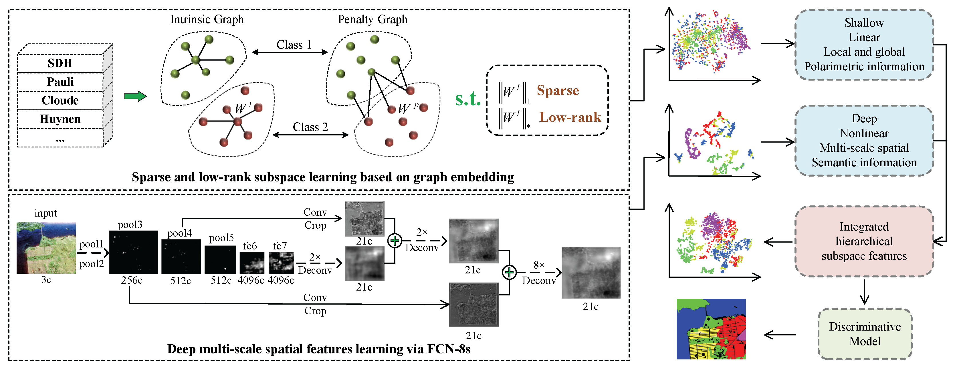
As a powerful semantic segmentation technique, FCNs [40] are trained end-to-end, pixels-to-pixels on the pre-trained VGG-16 classifier, which mainly consists of thirteen convolutional layers, three fully connected layers, and other basic components such as pooling and activation layers, etc., as shown at the first row in Figure 2. In the case of staged training, FCNs have three different architectures: the single-stream FCN-32s, the two-stream FCN-16s and the three-stream FCN-8s, as depicted at the second, third and fourth row in Figure 2, respectively. The difference among them lies in the fusion of layers with different depths.
To convert classification networks to fully convolutional networks for dense prediction, the following key operations are designed specially. Firstly, all fully connected layers are substituted by convolutional layers to ensure the nets can take arbitrary-sized inputs and produce 2D spatial outputs, where the fully connected layers just have fixed dimensions and generate a feature vector. Secondly, to output the same size as the input image, the fully convolutional layers are followed by several deconvolutional layers, since the output spatial dimensions of ahead layers are reduced by subsampling.
Subsequently, to further refine the spatial precision performance, a skip architecture is developed to combine fine layers and coarse layers. Specifically, as described in Figure 2, the fourth pooling layer is followed by “” layer containing a 1 × 1 convolution, and then the outputs of layer are element-wise summed with 2× upsampling of the final fully convolutional layer, thus yielding the two-stream FCN-16s after 16× upsampled. Similarly, the three-stream FCN-8s is generated by this way. Finally, the last classifier layer is discarded and a 1 × 1 convolution with channel dimension 21 (only for PASCAL VOC 2011 image set with 21 classes) is appended to predict score for each class.
2.3. Subspace Learning Based on Graph Embedding
Graph embedding (GE) proposed first in [41] refers to a general framework for dimensionality reduction, and it represents data and similarities between data with an undirected weighted graph. Specifically, each vertex of graph denotes a data point or a feature while the weight of edge represents similarity between the connected vertex pair, where similarity is measured by a graph adjacency matrix formed by using various similarity criteria. GE has three extensions: linearization, kernelization, and tensorization. Among of them, linearization is used to reduce dimension of PolSAR data in this paper, because of its empirical success in practice and its computational efficiency.
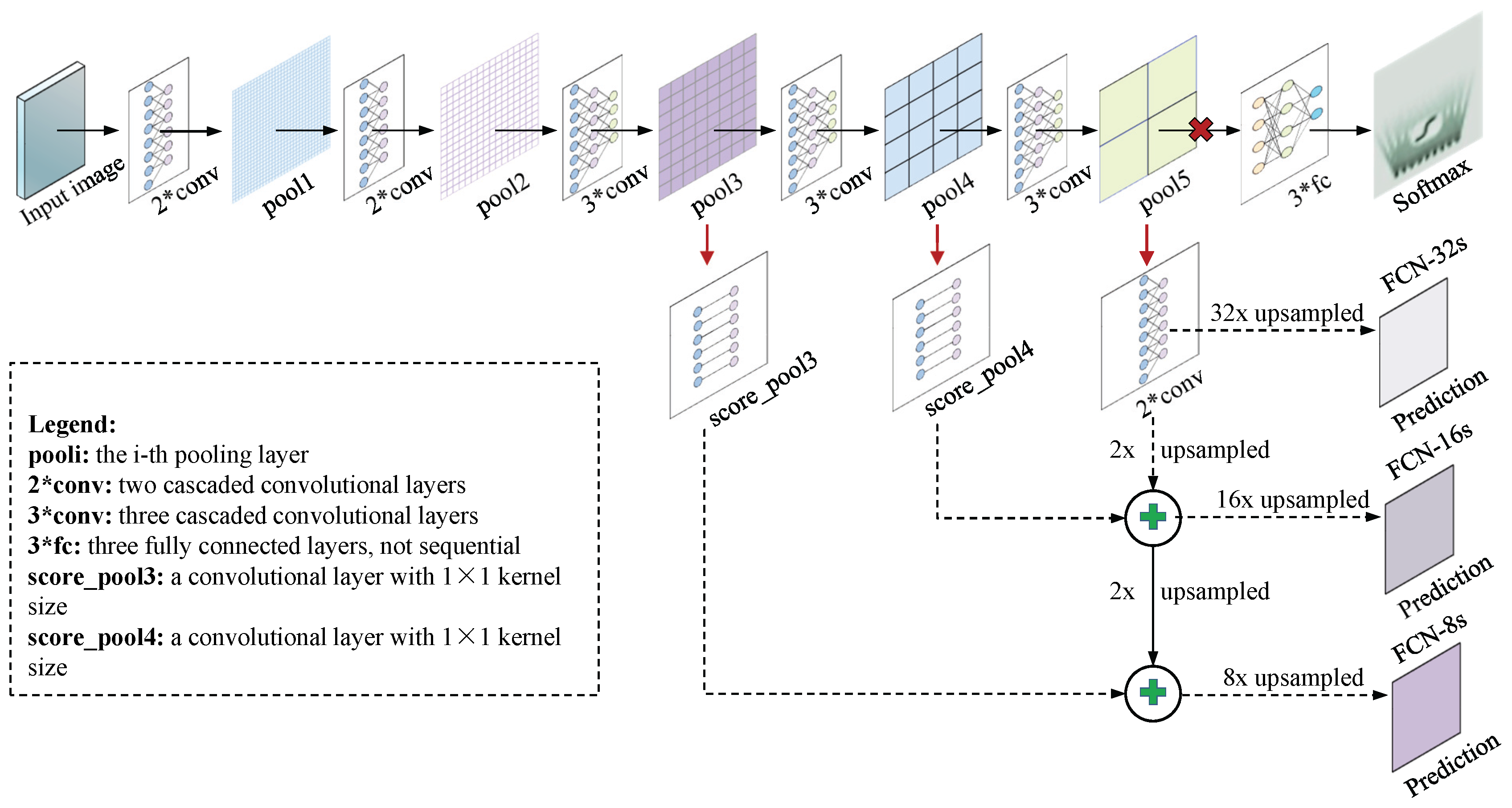
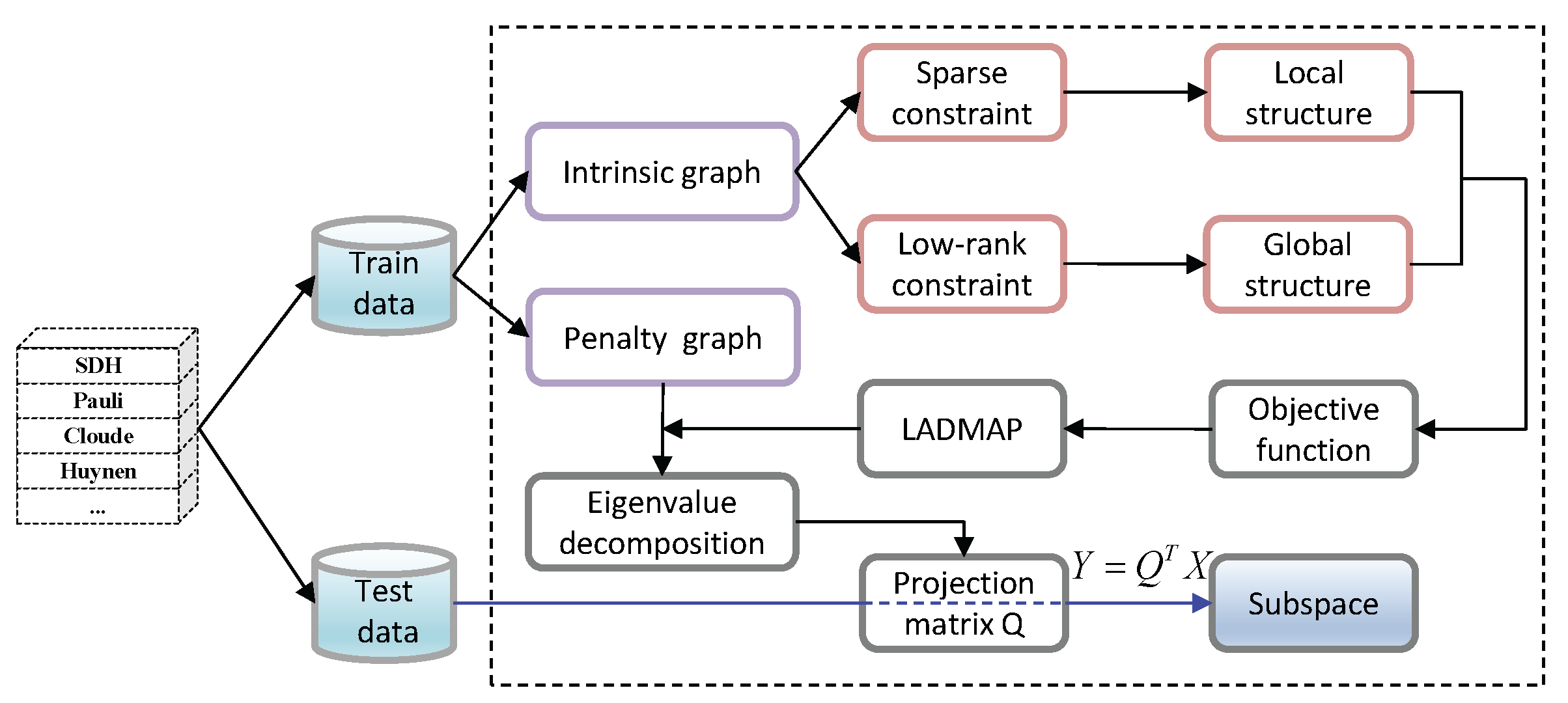
In GE, an intrinsic graph and a penalty graph are designed to characterize desired properties and suppressed properties in the dimension-reduced subspace, respectively. In the intrinsic graph, if two vertexes among the k1-nearest neighbor belong to the same class, then they are connected. On the contrary, in the penalty graph, the connected two vertexes among the k2-nearest neighbor are from different classes, as illustrated in Figure 3.
Given a training PolSAR data set containing M samples, denoted as , , where N is the dimension of the stacked polarimetric features, then an intrinsic graph and a penalty graph can be defined, where the real symmetric similarity matrix can be computed according to different similarity criteria, such as local neighborhood relationship [41], and the constraint matrix can optionally be an identity matrix for scale normalization. The linear version of GE aims to seek a projection matrix to project onto a low-dimensional subspace, which is , where , , is the subspace representation of , K denotes the dimension of subspace, and . In the dimension-reduced subspace, the similarity preservation property from the intrinsic graph should be measured by minimizing the distances of the vertex pairs from the same class, as well as maximizing the distances of vertex pairs that belongs to different classes. Therefore, the subspace learning algorithm based on GE can be formulated as:
where c is a constant. With some algebra, the objective function in Equation (5) is simplified as
where is Laplacian matrix of graph , defined as , is a diagonal matrix, whose diagonal elements . Laplacian matrix of graph is defined similarly. The optimal projection matrix can be represented as
The solutions of Equation (7) can be obtained by solving the following generalized eigenvalue decomposition problem:
where is eigenvalue matrix, and the feature vectors corresponding to the first K smallest eigenvalues constitute a K projection matrix . In essence, the difference of different subspace learning algorithms based on GE lies in the design of .
3. Integrating Hierarchical Subspace Features for PolSAR Image Classification
3.1. Sparse and Low-Rank Subspace Representations of PolSAR Data
As discussed in Section 1.1, SR and LRR can make significant contributions to enhance the discrimination of feature for classification. Therefore, we enforce the sparse and low-rank constraints on similarity matrix as done in [31] to reduce the dimension of PolSAR data. Specifically, the sparsity and low-rankness are implemented by -norm and nuclear-norm optimization problems, respectively. Thus, the objective function can be described as
where and denote the nuclear norm, -norm of matrix, respectively. is a parameter used to control the tradeoff between the nuclear norm and the -norm, and denotes the sparse representation based on dictionary . The column of intrinsic graph weight matrix denotes the sparse representation coefficient vector corresponding to atom of dictionary. To utilize class-label information, the similarity matrix is estimated by using within-class samples to generate class-specific sparse coefficients. To this end, is designed to be a block-diagonal matrix as follows:
where is the total number of class, denotes the weight matrix obtained by sparse representation only using labeled samples in the c-th class; here, is the number of samples of the c-th class, and . Thus, the subspace learning algorithm is called block SLGDA (BSLGDA). By introducing two auxiliary variables: similarity matrix and residual matrix , the objective function can be further simplified into
where is the -norm. This problem can be solved by the linearized alternating direction method with adaptive penalty (LADMAP) [42], which minimizes the following augmented Lagrangian function:
where and are Lagrangian multipliers, is a penalty parameter, denotes Frobenius norm, and . A natural way to solve the problem is to iteratively optimize Equation (12) over one variable, while fixing the others. Specifically, in the th iteration, the variables are first alternately updated by the following formula:
where is the singular value shrinkage operator [43], , and is soft-thresholding shrinkage operator, which is equal to: if , if , and 0 elsewhere. Subsequently, two Lagrangian multipliers are updated by
and those variables are updated alternately until the preset convergence condition is satisfied. For more details, we recommend readers to refer to [31,44].
Once the optimal similarity matrix is obtained, by specifying the identity matrix for and then solving Equation (8), we can perform DR on the high-dimensional stacked polarimetric features to acquire the sparse and low-rank feature representations in dimension-reduced subspace. Figure 4 illustrates the whole procedure of learning a low-dimensional sparse and low-rank subspace representations of PolSAR data based upon GE.
3.2. Deep Multi-Scale Spatial Features Learning via FCN-8s
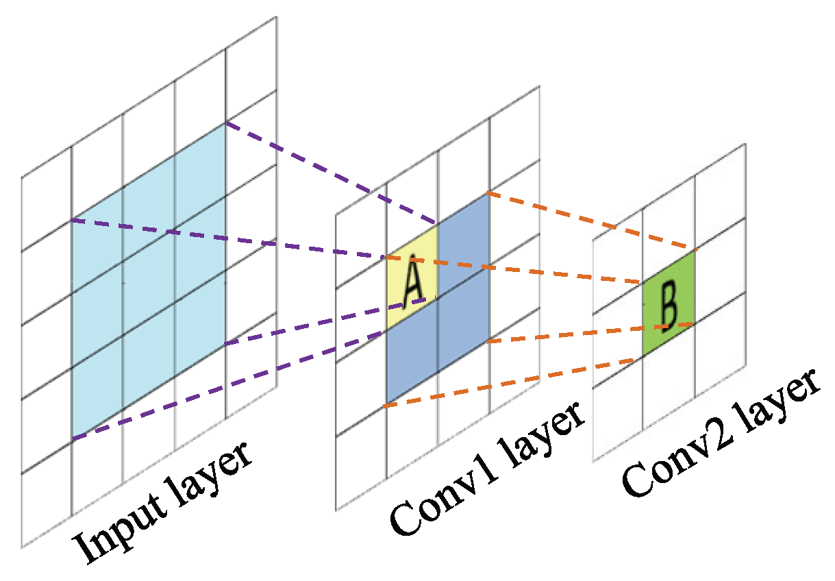
Different from the ordinary CNNs, FCNs can maintain the important 2D structure of the input image, which make it possible to learn spatial properties. In our work, this kind of superiority is used for PolSAR data analysis. Among of three architectures of FCNs mentioned in Section 2.2, FCN-8s is demonstrated in both theory and practice to perform best on semantic segmentation. To explain it, the receptive field (RF) is concerned. As shown in Figure 5, the RF of locations in higher layers refers to the specific region of the input image that they are path-connected to. From the top layer to down layer, the RF size of layer depends on the kernel sizes of top layers and the strides of top l layers. Writing for the RF of layer l, for the kernel size of layer , and for the stride of n-th layer, then the RF of layer can be computed by
where the RF of input layer is defined as . Obviously, the deeper the layer is, the larger the RF size will be. In FCN-8s, the kernel sizes of all the convolutional layers and pooling layers are 3 × 3 and 2 × 2, respectively, and the corresponding strides are 1 and 2. The skip architecture of FCN-8s, i.e., combining the shallower coarse layers and deep fine layers, determines it has multi-scale RFs, including 44, 100, 404, etc. [34]. Thus, FCN-8s has the potential to capture multi-scale local-to-global spatial features, due to the fact that shallow layers can learn local features while deep layers can learn global ones.
Let denote the three-dimensional input of l-th layer with pixel size , and channels, and denote the feature map of i-th channel in layer l, and then the outputs of feature map of j-th channel in layer can be computed by
where is the nonlinear Rectified Linear Units activation function. represents convolutional kernel of layer that connects the i-th map in layer l and the j-th map in layer , the kernel size is , denotes the bias of output j-th map in layer , and ∗ stands for convolutional operator. Equation (16) implies that FCN-8s can capture the nonlinear properties, which are very useful for PolSAR image classification.
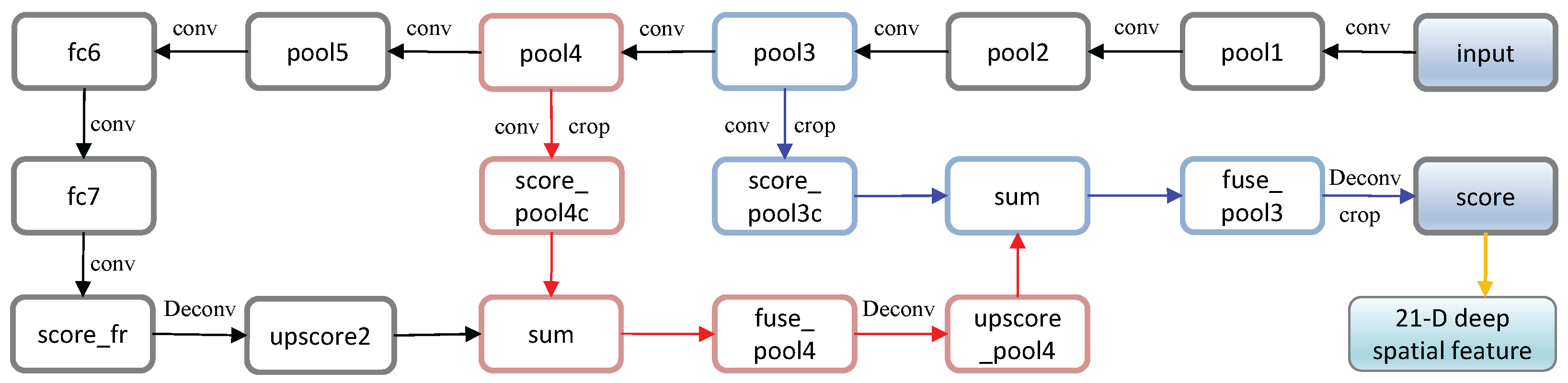
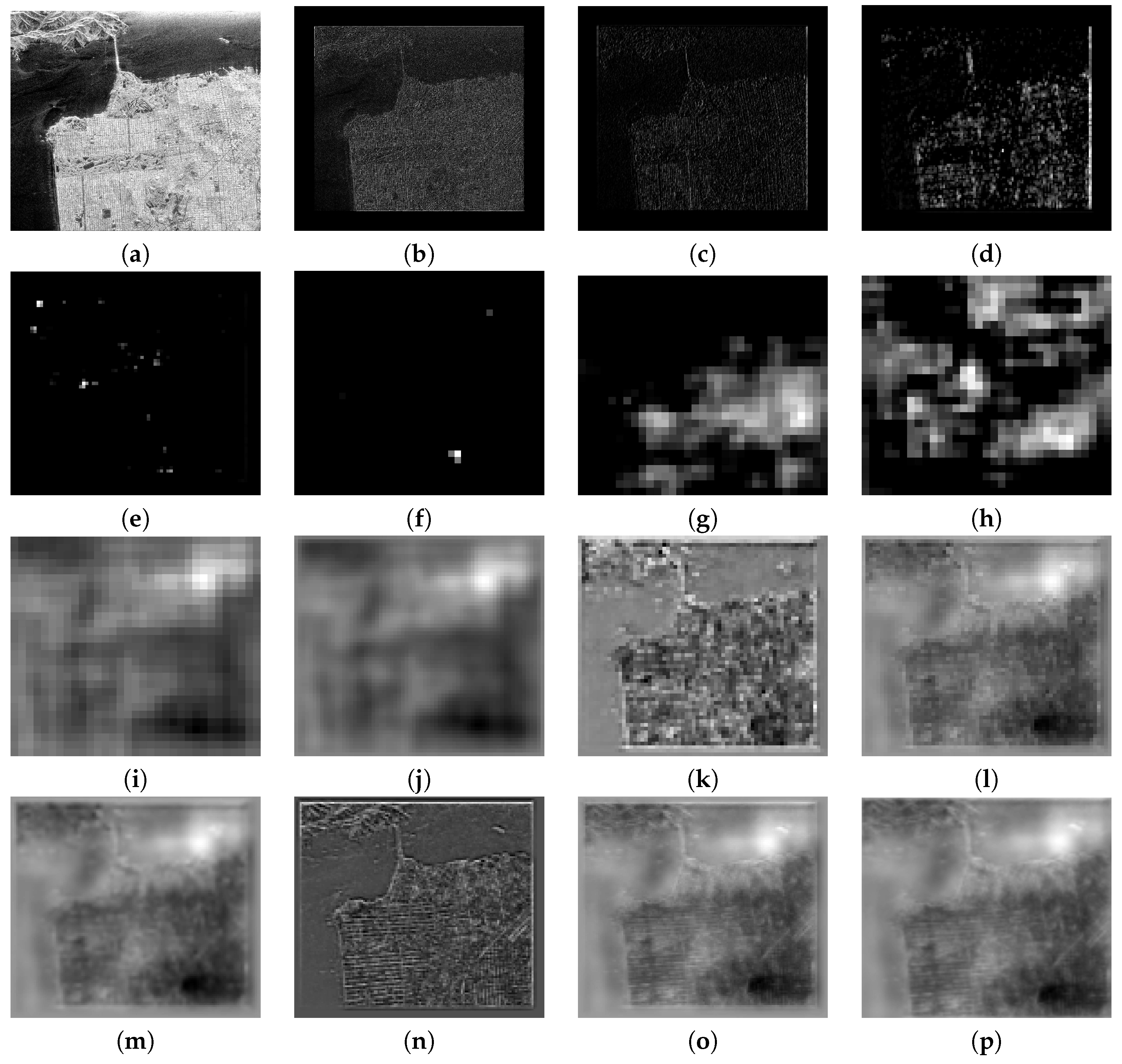
Motivated by the successful application of FCN-8s in hyperspectral image classification [34], we transfer the FCN-8s model pre-trained on PASCAL VOC 2011 image set to extract the potential deep structural information of PolSAR data. To match the pre-trained model parameters well, we input the Pauli-decomposed pseudo-color image of PolSAR data, whose “RGB” channels are , and , respectively. Figure 6 shows the procedure of extracting deep multi-scale spatial features of PolSAR data by FCN-8s, and the visual feature maps corresponding to the first channel of the major specific layers are displayed in Figure 7, where the Pauli pseudo-color image of San Francisco data is used as an example.
Comparing the visual feature maps of different layers in Figure 7, such as “” layer, “” layer and “upscore2” layer, it can be concluded that shallow layers are better at learning appearance features, while deep layers have advantages for obtaining the more abstract structure, and the combination of shallow layers and deep layers can refine the feature. For instance, the features of “” layer are finer than these of “” layer and “upscore2” layer, and “” layer contains more informative spatial features than “” layer. The final 21D deep spatial features from 21 kinds of different filters, i.e., the outputs of “score” layer, contain nonlinear multi-scale spatial information. Therefore, they are selected to facilitate PolSAR image classification in our work.
3.3. Integrating FCN with Sparse and Low-Rank Subspace Representations for PolSAR Imagery Classification
Actually, although FCN-8s has a powerful potential to learn nonlinear deep multi-scale spatial features, it is weak in processing boundary and other details, due to its relatively large RF. While SLGDA can capture more local details and global structures, but it is linear and lack of spatial constraints. Therefore, we integrate two types of features to make their individual advantages beneficial for each other with a weighted strategy. Considering that they have different dimensions and orders of magnitude, we employ Z-score to eliminate the effect following the idea in [34].
Let , denote deep spatial feature of M samples with dimension , where , and , represent the sparse and low-rank subspace feature with dimension ; then, the integrated hierarchical subspace feature can be represented as
where and are weighting factors, and
which computes Z-score of X, where and denote the mean value and standard deviation of X along the row, respectively, and subscript denotes the calculation is performed column-by-column. In feature , , each sample is represented by a -dimensional feature vector, which contains multiple types of information, ranging from low-level to high-level, linear to nonlinear, local to global, and polarimetric to multi-scale spatial.
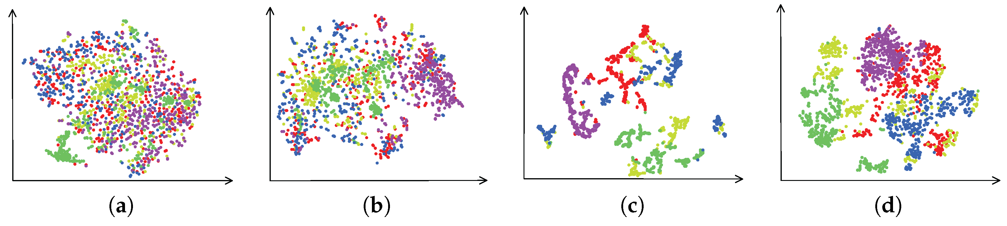
To investigate the discrimination of the learned feature, t-distributed stochastic neighbor embedding (t-SNE) [45] is used to visualize feature in a 2D space.
We conduct experiments on San Francisco data, and randomly select 300 samples of each class to be visualized. From the visualizations of different features shown in Figure 8, it can be observed that deep spatial features can make the intraclass samples become compact, but cannot separate the interclass samples very well. However, this problem can be improved when the sparse and low-rank subspace feature is incorporated, which indicates that the integrated hierarchical subspace features have powerful discrimination.
4. Experiment
4.1. Experimental Data Sets
To validate the effectiveness of the proposed classification scheme, we conduct experiments on several popular PolSAR data sets.
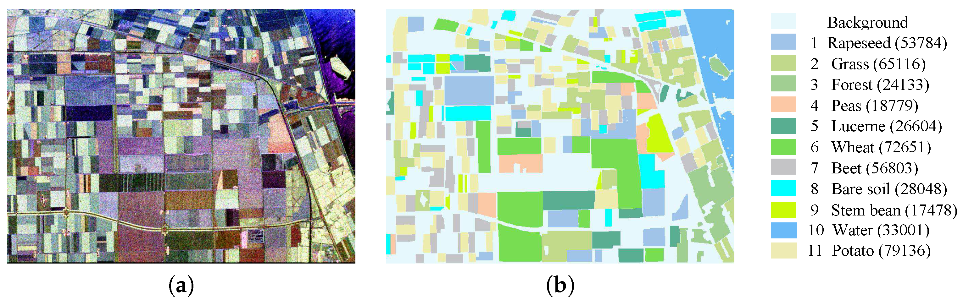
- Flevoland data set: The PolSAR data set of Flevoland is a subset of an L-band four-look image acquired by the NASA/Jet Propulsion Laboratory Airborne SAR (AIRSAR) platform in 1989. The data set measured 750 × 1024 pixels with a resolution of 12 m × 6 m, and it is divided into 11 classes referring to [12], where rapeseed, grass, forest, peas, Lucerne, wheat, beet, bare soil, stem beans, water and potato are included. For illustrative purposes, the Pauli-decomposed pseudo-color image and its corresponding ground truth are shown in Figure 9.
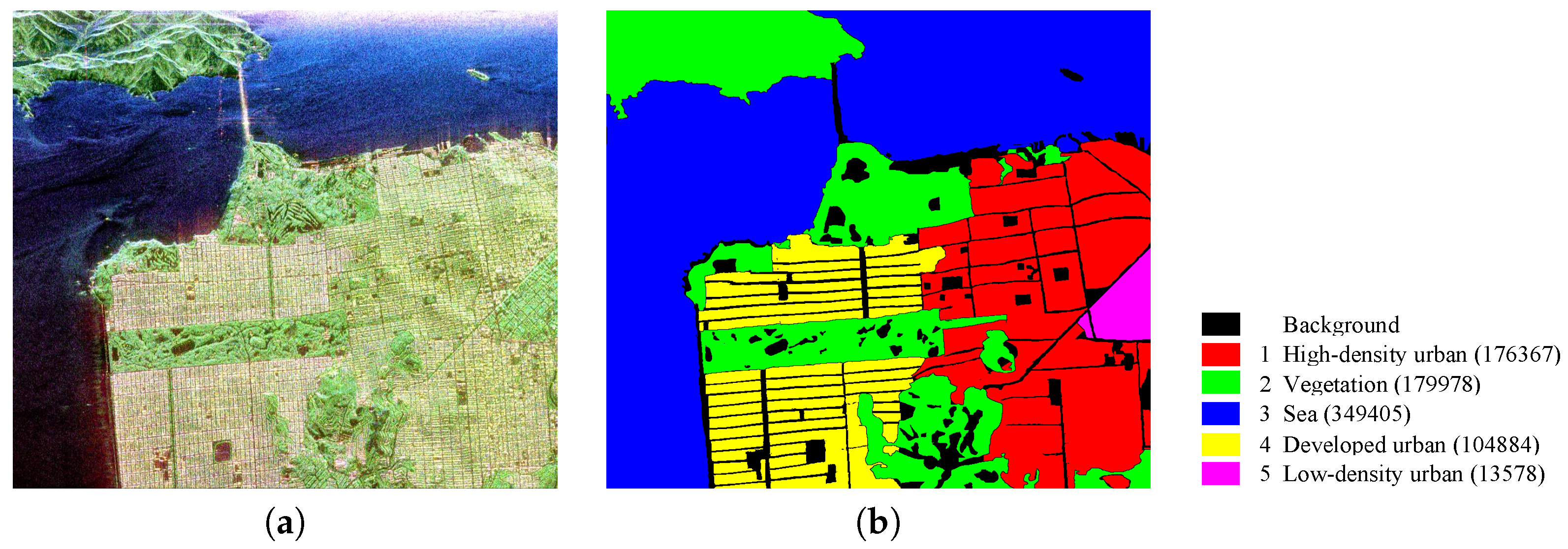
- San Francisco data set: The PolSAR data of San Francisco Bay area, acquired by the NASA/Jet Propulsion Laboratory AIRSAR at L-band, consists of five kinds of terrain types: water, mountain, three types of urban areas. This polarimetric SAR data has a size of 900 × 1024 pixels, and its spatial resolution is about 10 m × 10 m. The Pauli color coded image and its ground truth are given in Figure 10.
- Flevoland Benchmark data set: The third PolSAR data used for validation is the benchmark data set of an L-band AIRSAR data obtained in 1991 over Flevoland. The selected image covers a size of 1020 × 1024 pixels, and Figure 11 shows the Pauli-decomposed pseudo-color image and its corresponding ground truth, respectively, where the ground truth comes from [21]. The ground truth shows that the benchmark data contain 14 classes.
4.2. Experiment Settings and Parameters Analysis
4.2.1. Experiment Settings
In each experiment, we randomly select a certain percentage of polarimetric data mentioned in Section 2.1 as training set, and the remaining samples are used for testing. Then, the training set is used to construct an intrinsic graph and a penalty graph, which are used to learn a linear projection relationship from the polarimetric feature space to a low-dimensional subspace with BSLGDA. Next, the test set is directly projected onto the subspace by .
Meanwhile, the Pauli color coded images of training and test sets are fed into an FCN-8s model pre-trained on PASCAL VOC 2011 image set to extract the 21-dimensional deep multi-scale spatial features. Afterwards, the spatial features are integrated with the shallow sparse and low-rank subspace features by a weighted way. Finally, a discriminative model, i.e., SVM with Gaussian kernel, is well trained to obtain the class label of testing samples.
In order to robustly evaluate the classification performance of the proposed algorithm, we randomly select the samples and repeat the experiments ten times per data set. The overall accuracy (OA) of classification, Kappa coefficient and confusion matrix are used for evaluation. For comparison, we conduct extensive experiments with different features derived from the following algorithms:
- BSLGDA: only employ BSLGDA to learn the low-dimensional sparse and low-rank representations of high-dimensional polaimetric features, which are linear and shallow from the point of view of DL feature, where spatial features are not concerned.
- FCN: only transfer the pre-trained FCN-8s to extract deep multi-scale spatial structural information of Pauli-decomposed pseudo-color image, which are nonlinear and high-level abstract spatial representations.
- PCA + FCN: use the traditional principal component analysis (PCA) to perform DR on high-dimensional polaimetric features, then integrate PCA features with FCN features by using a weighted strategy.
- BSLGDA + FCN: integrate shallow sparse and low-rank subspace representations of high-dimensional polaimetric features with deep multi-scale spatial features by using a weighted strategy.
- BLGDA+FCN: use block low-rank graph embedding discriminative analysis (BLGDA) to perform DR. Compared with BSLGDA+FCN, the only difference lies in that sparsity is not concerned.
- BSGDA+FCN: use block sparse graph embedding discriminative analysis (BSGDA) to complete DR. Compared with BSLGDA+FCN, the only difference lies in that low-rankness is not considered.
4.2.2. Parameters Tuning
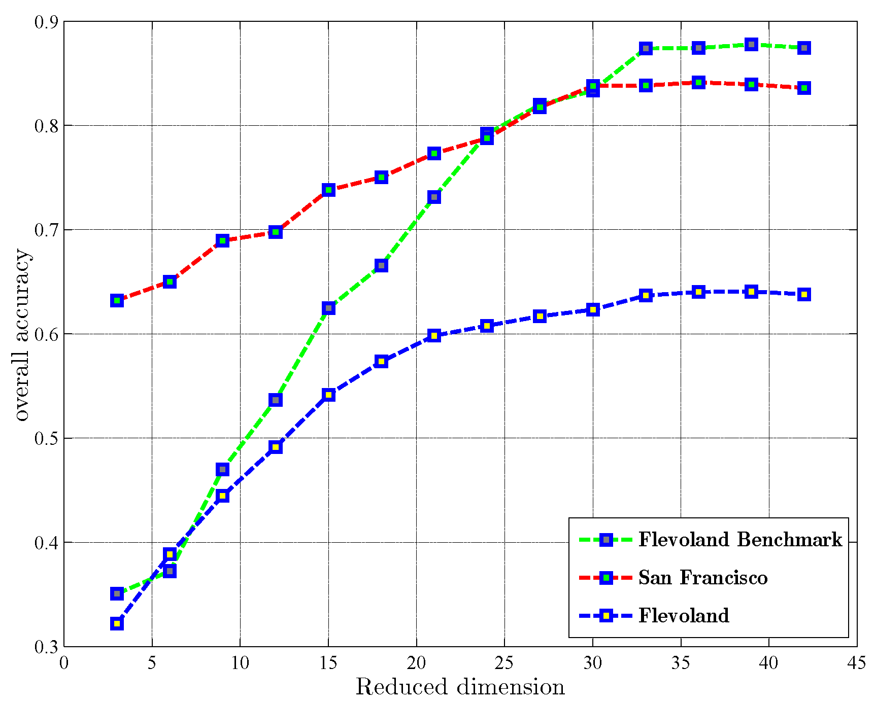
The proposed classification scheme involves several major parameters, and they are well tuned before classification with cross-validation strategy. At the DR stage, in the BSLGDA, the regularization parameter and are empirically set to 0.5 and 0.001, when , the BSLGDA degenerates into the BLGDA. The parameters in BSGDA are set according to the original publication [31]. To find an appropriate reduced dimension of subspace for BSLGDA, 1% labeled samples are randomly selected from each class, and the rest are used for testing. Then, the classification OA curves with respect to the reduced dimension by using BSLGDA on three PolSAR data are shown in Figure 12. According to the curves, the reduced-dimensionality for Flevoland, San Francisco and Flevoland Benchmark data sets are set to 33, 30 and 33, respectively. For a fair contrast, the other comparing methods are tuned to their optimum dimensions.
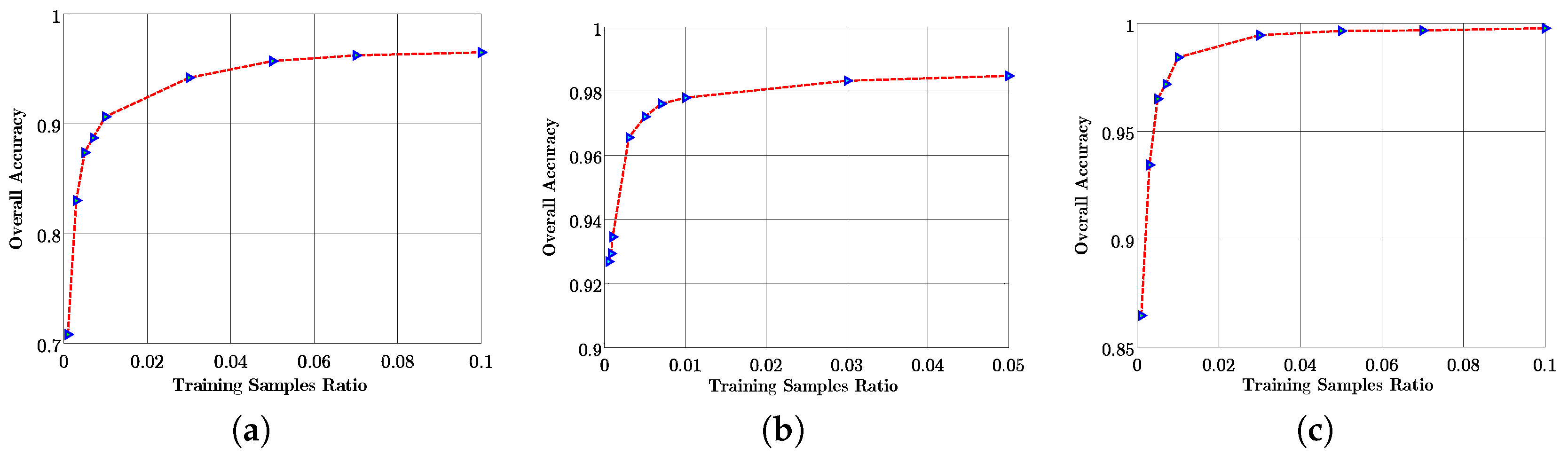
Furthermore, to seek a proper rate of training samples for the proposed BSLGDA+FCN algorithm, we change the ratio in the optimal reduced-dimensionality, and obtain the classification OA curves with respect to different training sample rates, as displayed in Figure 13. Taking into account both accuracy and time cost, the training rates of each class are set to 5%, 3% and 5% for Flevoland, San Francisco and Flevoland Benchmark data sets, respectively.
At the stage of integrating hierarchical subspace features, the weighting factors and are chosen between 0 and 1 with a stride 0.1. Empirically, they are set to 0.8 and 0.2, respectively. When , , only spatial features learned by FCN are used, and when , , only the features learned by BSLGDA are employed. Finally, a Gaussian kernel of SVM is tuned to be optimal by cross-validation.
4.3. Classification Performance
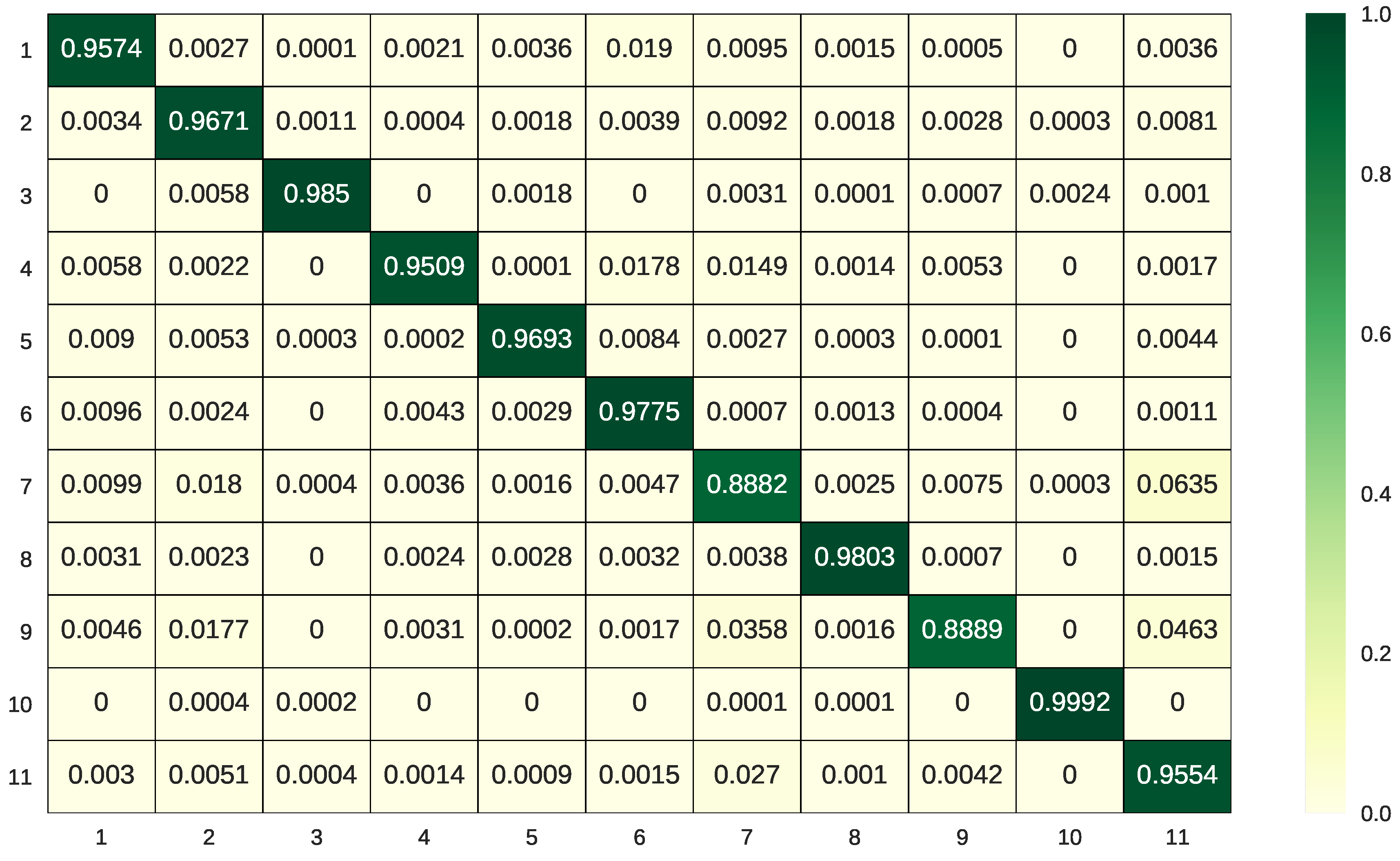
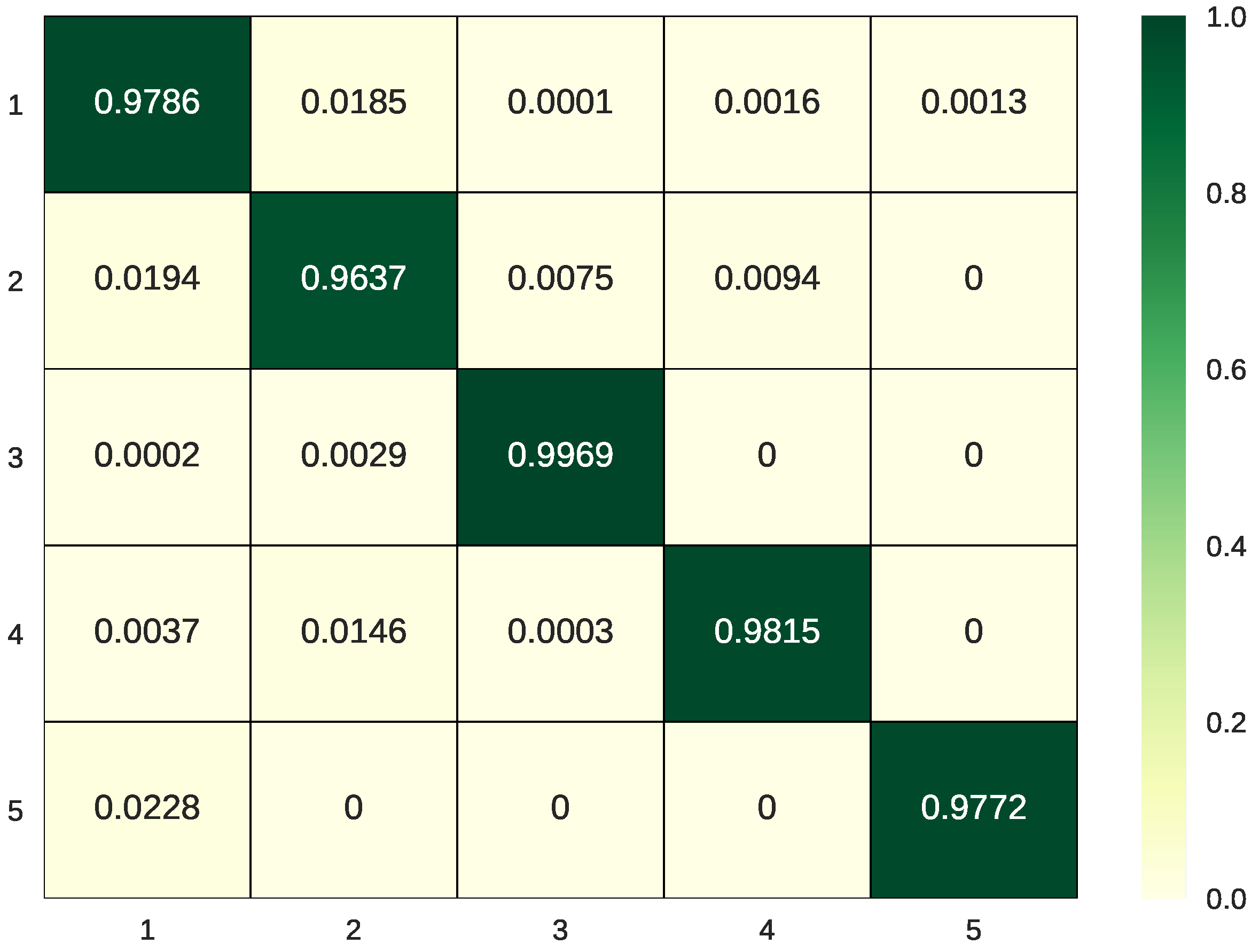
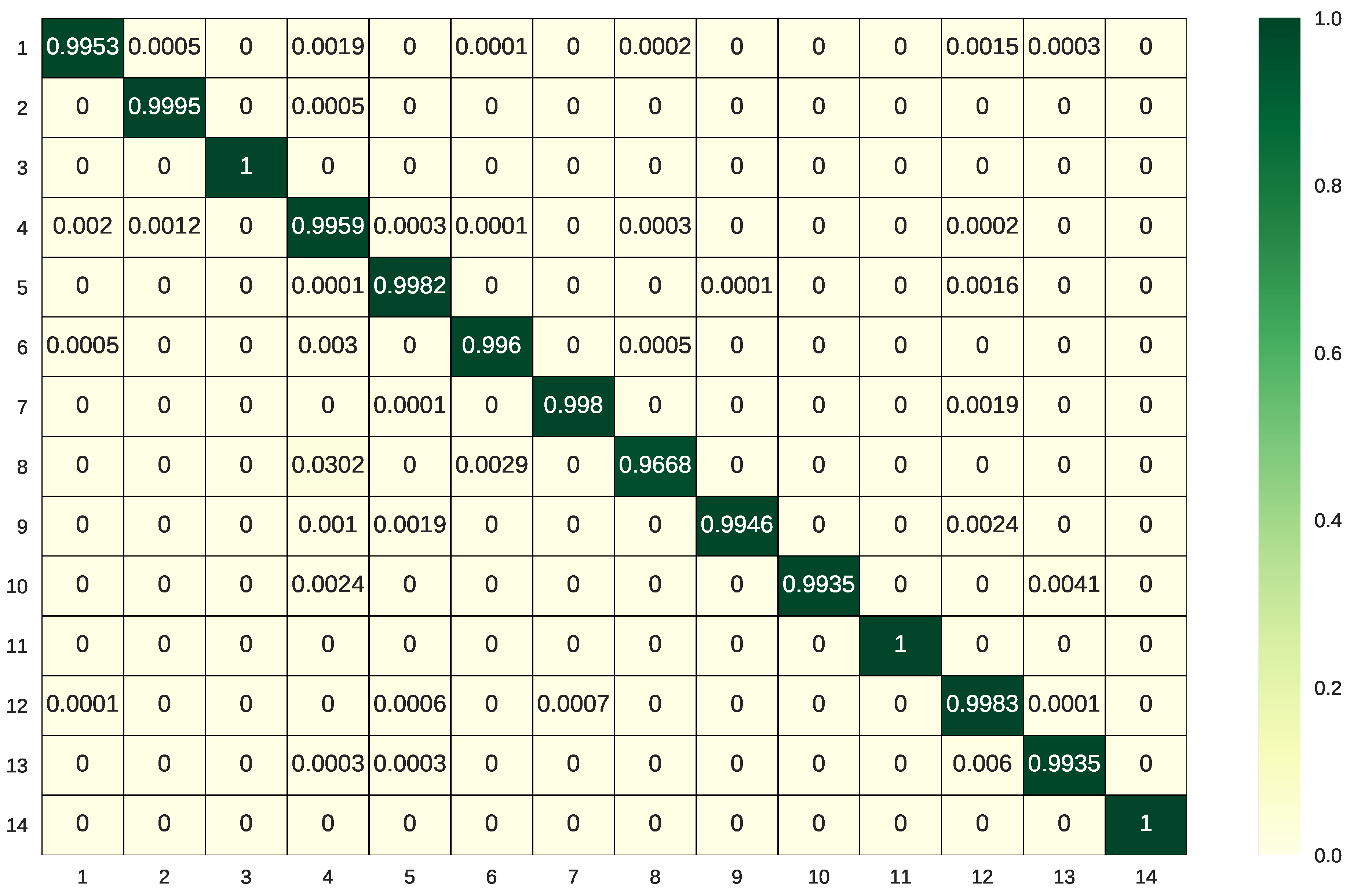
In this section, we report the classification performance of the proposed BSLGDA+FCN and other methods for comparison on three PolSAR data. Specifically, the class-specific accuracy, OA and Kappa coefficient are listed in Table 1, Table 2 and Table 3 for the Flevoland, San Francisco and Flevoland Benchmark data, respectively. Accordingly, the classification confusion matrix based on the proposed method are presented in Figure 14, Figure 15 and Figure 16, and Figure 17, Figure 18 and Figure 19 show the visual classification results for the three experimental data.
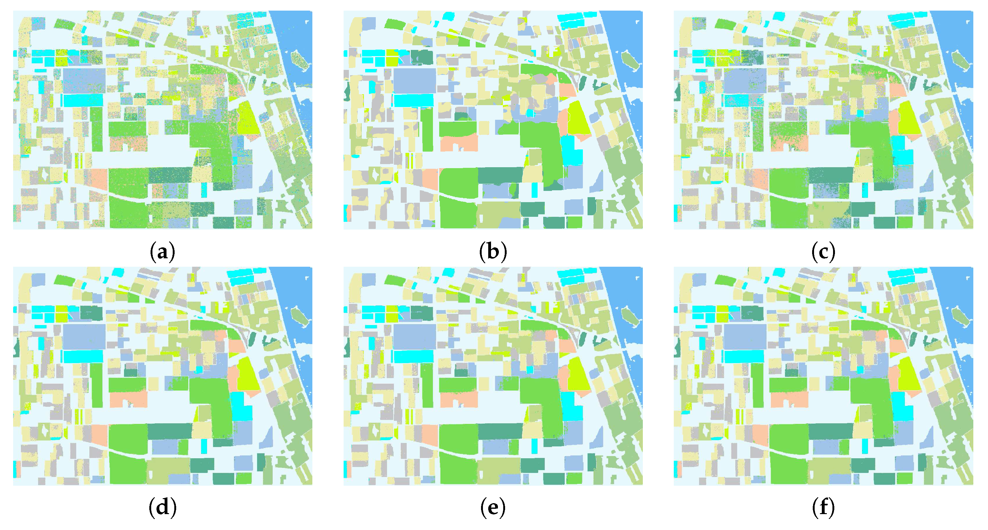
For the Flevoland data set, the classification results given in Table 1 show that BSLGDA performs worst almost on every class, the OA is low as 73.77%, which can be explained by its linearity and lack of spatial constraints. While FCN can offer a higher OA of 90.99%, it performs well except for on Beet (class 7) and Stem Bean (class 9), where the accuracy for Stem Bean , 71.13% , is even lower than that of BSLGDA, 71.70% . By contrast, the integration of deep spatial features learned by FCN with the features learned via graph embedding discriminative analysis (GDA), whether it is BLGDA, BSGDA or BSLGDA, can greatly improve the accuracy almost for all classes, especially for Beet, Stem Bean and Potato (class 11), the accuracy is about 11%, 17%, and 4% higher than that of FCN, respectively. This indicates that the shallow sparse and (or) low-rank subspace representations can boost the discrimination of deep multi-scale spatial features. Among the three GDAs, BLGDA + FCN has the highest OA of 96.12%, and BSLGDA + FCN is the second best on most of classes. However, not all of the synergies of subspace methods with FCN can perform well. For instance, compared with FCN, the PCA + FCN just benefits for Beet, Stem Bean and Potato while worsening the performance on other classes, the OA is reduced by 9.02%.
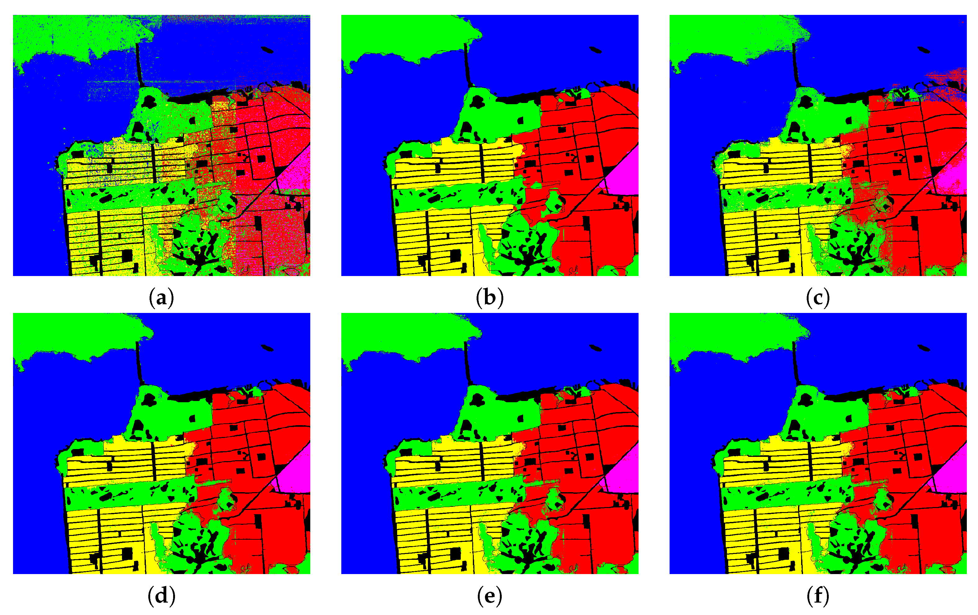
For the San Francisco data, the classification results listed in Table 2 indicate that integration of FCN with GDAs can offer a higher OA than BSLGDA, 86.51%, and FCN, 97.82%. Even if FCN has outperformed BSLGDA far away, the accuracies for all the classes are higher than 95% and that for Sea (class3) reaches to 99.44%, which demonstrates that deep spatial structural features learned via FCN can make a great contribution to distinguish different classes. However, from the visual classification results shown in Figure 18b, it can be obviously observed that there are a lot of incorrectly classified pixels on the border, such as the junction of areas represented by yellow and green, due to the fact that FCN cannot deal with boundary well. Fortunately, the weakness of FCN can be greatly improved by incorporating sparse and (or) low-rank subspace representations into FCN features. The cooperation of FCN with BLGDA, BSGDA, and BSLGDA improves the OA up to 98.38%, 98.04% and 98.34%, respectively, and they have almost the same performance. Figure 15 shows the classification confusion matrix based on BSLGDA+FCN, which illustrates that only a few pixels are wrongly classified by using the proposed scheme. However, it is worth noting that PCA+FCN makes results worse instead of facilitating classification, which suggests that the integrated subspace features of FCN and PCA are not beneficial for PolSAR image classification.
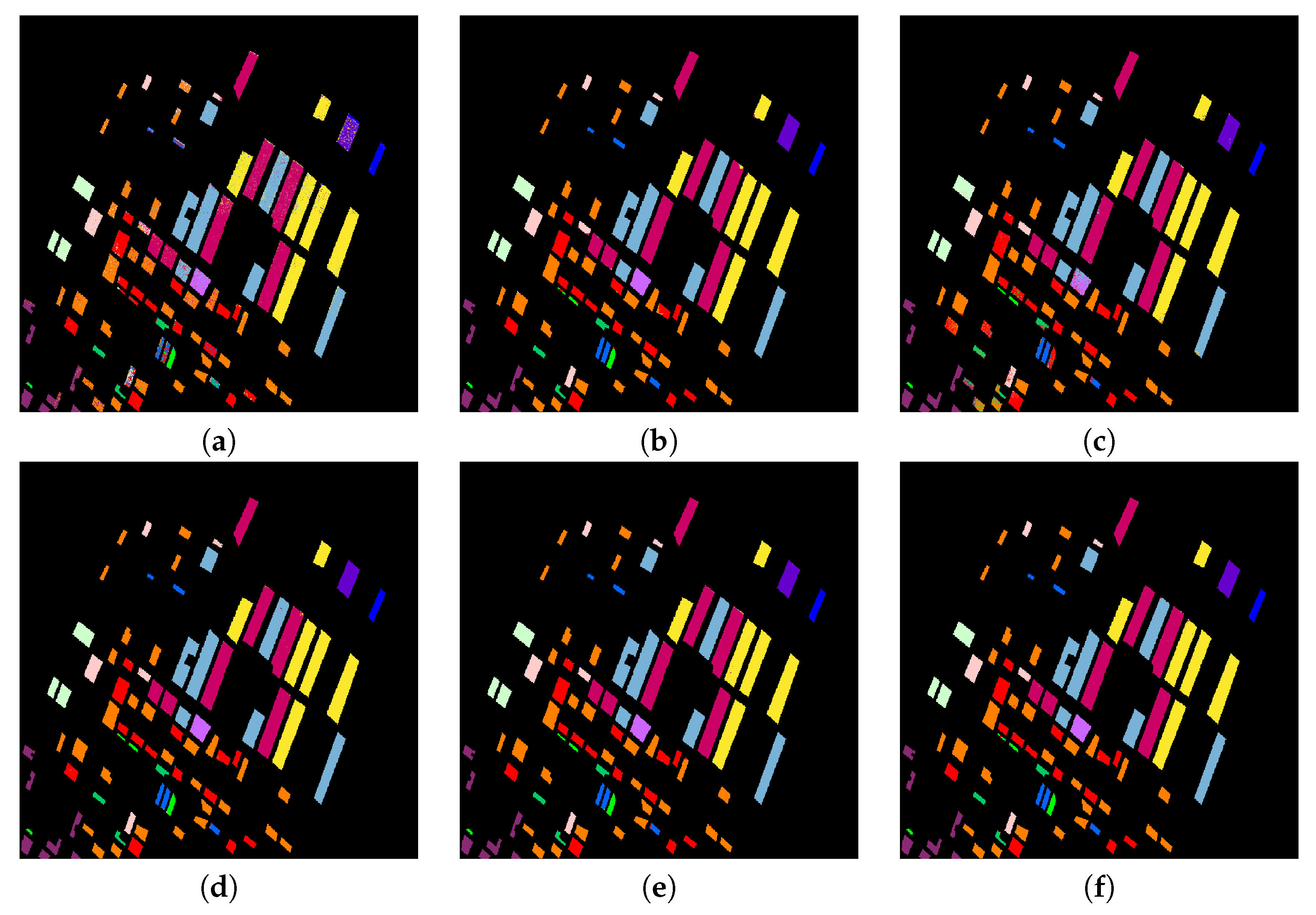
Figure 19 shows the visual classification results on Flevoland Benchmark data, and the accuracy for each class, OA and Kappa coefficient corresponding to different algorithms are listed in Table 3. Although the sparse and low-rank subspace representations can achieve a high OA of 92.80%, when integrated with deep spatial information, the better classification performance, an OA of 99.72%, can be obtained. The proposed BSLGDA+FCN has the best visual effect and the highest accuracy 99.46% and 99.83% for Peas (class 9) and Rapeseed (class 12), respectively. Figure 16 demonstrates the classification confusion matrix of the proposed method, and this clearly indicates the almost perfect performance of BSLGDA+FCN on every terrain. Particularly, BSLGDA+FCN achieves an accuracy of 100% for Oats (class 3), Flax (class 11) and Lucerne (class 14). Moreover, compared with the FCN, the accuracy 90.54% for Beans (class 8) is increased to 99.51% by BSGDA + FCN. Actually, taking the randomness into account, the tiny differences in accuracy of BSLGDA + FCN, BLGDA + FCN and BSGDA + FCN are negligible, that is to say, all the integrations of FCN with three GDAs obtain comparable results on Flevoland Benchmark data. Although the FCN alone has excellent performance, i.e., a very high OA of 97.45%, the synergy effect can maximize the accuracy. However, the classification OA, 96.49%, by using PCA+FCN indicate that the subspace features from PCA are not fit for being incorporated into FCN features to facilitate the classification.
Finally, the computational time of the proposed algorithm and other methods for comparison are given in Table 4 and Table 5. Except for the experiment that extracts deep multi-scale spatial structural features by FCN-8s is conducted under the Caffe framework on a NVIDIA Tesla K40 GPU, the execution time is 60.44 s, 70.14 s and 79.98 s for Flevoland, San Francisco and Flevoland Benchmark data sets, respectively. Table 4 shows an approximately linear relationship exists between pixels and execution time. The other experiments are implemented using MATLAB 2014 on an Intel Core i5-4570 CPU machine with 32 GB of RAM. The execution time presented in Table 5 demonstrates that the single FCN and PCA + FCN have much lower computational costs, while the cost of BSGDA + FCN is the highest due to the fact that BSGDA is solved by interior-point method in [46], which takes a huge amount of time. In contrast, although BSLGDA + FCN and BLGDA + FCN have medium computational time cost, they also take too much time due to the solving method, i.e., LADMAP, involves singular value decomposition, which is time-consuming and takes up most of the time. Therefore, a faster method for solving BSLGDA remains to be studied to speed up the proposed method.
5. Discussion
This paper has presented an effective classification scheme for PolSAR image, which integrates deep multi-scale spatial information learned by FCN-8s model with shallow sparse and low-rank subspace representations. In the extensive experiments on three PolSAR data sets, the following interesting points are revealed.
- The influence of different reduced-dimension. Figure 12 indicates the variation in classification accuracy with respect to the reduced dimension by using the introduced BSLGDA under 1% training samples. It shows that the overall accuracies for Flevoland and Flevoland Benchmark data tend to be stable when the reduced dimension is larger than 33, while the reduced-dimensionality 30 for San Francisco data is a breaking point.
- The sensibility to different training rates. Figure 13 illustrates how the number of training samples affects the classification accuracy of the proposed BSLGDA+FCN. For Flevoland and Flevoland Benchmark data sets, when the training samples ratio is as low as 1%, the proposed method can still offer a high OA of more than 90%. When the ratio is more than 5%, the OA is satisfied and becomes stable. As for San Francisco data, an increase in the training rate leads to a higher accuracy until the rate reaches to 3%. It is worth noting that a very high accuracy can be achieved at a small training ratio, which indicates that the proposed method can perform well when the available training samples are limited. In other words, the proposed algorithm can tackle the small size samples problem effectively.
- The role of features learned via FCN-8s. The experimental results of using the single FCN features for classification demonstrate the great contribution of FCN features to improve classification, which can be explained by the nonlinear, deep-level and multi-scale structural properties learned adaptively from data by FCN. Moreover, in the experiments of integrated features, FCN features play a critical role in improving accuracy. However, FCN features are weak at coping with boundaries and other details, due to the fact that the FCN-8s model has relatively large receptive fields, which determine that it fails to obtain more detailed information.
- The role of sparse and low-rank representations. The sparse and low-rank constraints in BSLGDA make it possible to learn the local and global features. When incorporated into FCN features, the sparse and low-rank subspace features can effectively alleviate the boundary and other detail problems occurring in FCN. However, this kind of low-level learning features cannot offer a very high accuracy because BSLGDA is a linear subspace learning while PolSAR image classification belongs to a nonlinear mapping problem. Therefore, a nonlinear subspace learning based on GE should be further studied for enhancing the performance.
- The synergy effect of FCN and BSLGDA. In order to achieve the further improvement, this work resorts to a synergy of a pre-trained FCN-8s model with sparse and low-rank representations. The proposed BSLGDA+FCN utilizes the complementary advantages of FCN and BSLGDA to boost the discrimination of integrated hierarchical subspace features, which contain multiple types of information, including linear and nonlinear, shallow and deep, local and global, polarimetric and spatial properties. Thus, the synergy effect of FCN and BSLGDA significantly improves the classification accuracy.
- The main idea of the proposed method is not just limited to the integration of FCN and BSLGDA, and the success of our method can offer a general framework to integrate any other existing available methods that are consistent with our integration theory, as well as to develop new algorithms. However, the proposed method is supervised, and it requires tuning several parameters manually. Therefore, one of our future research works will concentrate on embedding the sparse and low-rank subspace features into FCN so as to automatically learn all the parameters. The current valuable results will lay down a solid foundation for studying an automatic classification network.
6. Conclusions
In this paper, we have proposed a hierarchical fully convolutional network integrated with the shallow sparse and low-rank subspace representations for PolSAR imagery classification. In terms of the classification accuracy, the proposed method can achieve a comparable result to that of the state-of-the-art methods without post-processing. In addition, for the data set with small size samples, the proposed method is very fast and efficient. On the one hand, the success of our method mainly relies on the powerful potential of FCN to automatically learn the nonlinear deep multi-scale spatial information. On the other hand, the subspace learning based on sparse and low-rank graph embedding discriminative analysis can uncover the intrinsic local and global structures of PolSAR data in a reduced-dimensional subspace. Most importantly, the effective synergy of deep FCN and shallow BSLGDA can make their respective advantages beneficial for each other, thus boosting the representation and discrimination ability of the integrated hierarchical subspace features.
However, BSLGDA is a linear subspace learning algorithm, and thus has many limits for nonlinear PolSAR image classification. Therefore, exploring an effective nonlinear subspace learning and its integration with an FCN model will be one of our future focuses.
Acknowledgments
This work was partially supported by the National Natural Science Foundation of China (No. 41371342, No. 61331016), and by the National Key Research and Development Program of China (No. 2016YFC0803003-01).
Author Contributions
Yan Wang and Chu He conceived and designed the experiments; Yan Wang performed the experiments and analyzed the results; Yan Wang wrote the paper; and Chu He, Xinlong Liu and Mingsheng Liao revised the paper.
Conflicts of Interest
The authors declare no conflict of interest.
References
- Ma, X.; Shen, H.; Yang, J.; Zhang, L.; Li, P. Polarimetric-spatial classification of SAR images based on the fusion of multiple classifiers. IEEE J. Sel. Top. Appl. Earth Obs. Remote Sens. 2014, 7, 961–971. [Google Scholar]
- Lee, J.S.; Grunes, M.R.; Kwok, R. Classification of multi-look polarimetric SAR imagery based on complex Wishart distribution. Int. J. Remote Sens. 1994, 15, 2299–2311. [Google Scholar] [CrossRef]
- Kong, J.A.; Swartz, A.A.; Yueh, H.A.; Novak, L.M.; Shin, R.T. Identification of Terrain Cover Using the Optimum Polarimetric Classifier. J. Electromagn. Waves Appl. 1988, 2, 171–194. [Google Scholar]
- Van Zyl, J.J. Unsupervised classification of scattering behavior using radar polarimetry data. IEEE Trans. Geosci. Remote Sens. 1989, 27, 36–45. [Google Scholar] [CrossRef]
- Cloude, S.R.; Pottier, E. An entropy based classification scheme for land applications of polarimetric SAR. IEEE Trans. Geosci. Remote Sens. 1997, 35, 68–78. [Google Scholar] [CrossRef]
- Lee, J.S.; Grunes, M.R.; Ainsworth, T.L.; Du, L.J.; Schuler, D.L.; Cloude, S.R. Unsupervised classification using polarimetric decomposition and the complex Wishart classifier. IEEE Trans. Geosci. Remote Sens. 1999, 37, 2249–2258. [Google Scholar]
- Ferro-Famil, L.; Pottier, E.; Lee, J.S. Unsupervised classification of multifrequency and fully polarimetric SAR images based on the H/A/Alpha-Wishart classifier. IEEE Trans. Geosci. Remote Sens. 2001, 39, 2332–2342. [Google Scholar] [CrossRef]
- Lee, J.S.; Grunes, M.R.; Pottier, E.; Ferro-Famil, L. Unsupervised terrain classification preserving polarimetric scattering characteristics. IEEE Trans. Geosci. Remote Sens. 2004, 42, 722–731. [Google Scholar]
- Dong, Y.; Milne, A.K.; Forster, B.C. Segmentation and classification of vegetated areas using polarimetric SAR image data. IEEE Trans. Geosci. Remote Sens. 2001, 39, 321–329. [Google Scholar] [CrossRef]
- Wu, Y.; Ji, K.; Yu, W.; Su, Y. Region-based classification of polarimetric SAR images using Wishart MRF. IEEE Geosci. Remote Sens. Lett. 2008, 5, 668–672. [Google Scholar] [CrossRef]
- He, C.; Liu, X.; Feng, D.; Shi, B.; Luo, B.; Liao, M. Hierarchical Terrain Classification Based on Multilayer Bayesian Network and Conditional Random Field. Remote Sens. 2017, 9, 96. [Google Scholar] [CrossRef]
- Qin, F.; Guo, J.; Sun, W. Object-oriented ensemble classification for polarimetric SAR Imagery using restricted Boltzmann machines. Remote Sens. Lett. 2017, 8, 204–213. [Google Scholar] [CrossRef]
- Zhang, L.; Ma, W.; Zhang, D. Stacked sparse autoencoder in PolSAR data classification using local spatial information. IEEE Geosci. Remote Sens. Lett. 2016, 13, 1359–1363. [Google Scholar] [CrossRef]
- Hou, B.; Kou, H.; Jiao, L. Classification of polarimetric SAR images using multilayer autoencoders and superpixels. IEEE J. Sel. Top. Appl. Earth Obs. Remote Sens. 2016, 9, 3072–3081. [Google Scholar] [CrossRef]
- Zhu, X.X.; Tuia, D.; Mou, L.; Xia, G.S.; Zhang, L.; Xu, F.; Fraundorfer, F. Deep learning in remote sensing: A review. arXiv, 2017; arXiv:1710.03959. [Google Scholar]
- Xie, H.; Wang, S.; Liu, K.; Lin, S.; Hou, B. Multilayer feature learning for polarimetric synthetic radar data classification. In Proceedings of the 2014 IEEE International Geoscience and Remote Sensing Symposium (IGARSS), Bryan, TX, USA, 13–18 July 2014; pp. 2818–2821. [Google Scholar]
- Geng, J.; Fan, J.; Wang, H.; Ma, X.; Li, B.; Chen, F. High-resolution SAR image classification via deep convolutional autoencoders. IEEE Geosci. Remote Sens. Lett. 2015, 12, 2351–2355. [Google Scholar] [CrossRef]
- Geng, J.; Wang, H.; Fan, J.; Ma, X. Deep Supervised and Contractive Neural Network for SAR Image Classification. IEEE Trans. Geosci. Remote Sens. 2017, 55, 2442–2459. [Google Scholar] [CrossRef]
- Lv, Q.; Dou, Y.; Niu, X.; Xu, J.; Xu, J.; Xia, F. Urban land use and land cover classification using remotely sensed SAR data through deep belief networks. J. Sens. 2015, 2015, 10. [Google Scholar] [CrossRef]
- Zhou, Y.; Wang, H.; Xu, F.; Jin, Y.Q. Polarimetric SAR image classification using deep convolutional neural networks. IEEE Geosci. Remote Sens. Lett. 2016, 13, 1935–1939. [Google Scholar] [CrossRef]
- Zhang, Z.; Wang, H.; Xu, F.; Jin, Y.Q. Complex-valued convolutional neural network and its application in polarimetric SAR image classification. IEEE Trans. Geosci. Remote Sens. 2017, 55, 7177–7188. [Google Scholar] [CrossRef]
- Wang, Y.; Wang, C.; Zhang, H. Integrating H-A-α with fully convolutional networks for fully PolSAR classification. In Proceedings of the International Workshop on Remote Sensing with Intelligent Processing (RSIP), Shanghai, China, 19–21 May 2017; pp. 1–4. [Google Scholar]
- Long, J.; Shelhamer, E.; Darrell, T. Fully convolutional networks for semantic segmentation. In Proceedings of the IEEE Conference on Computer Vision and Pattern Recognition, Boston, MA, USA, 7–12 June 2015; pp. 3431–3440. [Google Scholar]
- Zhang, L.; Zhang, L.; Du, B. Deep learning for remote sensing data: A technical tutorial on the state of the art. IEEE Geosci. Remote Sens. Mag. 2016, 4, 22–40. [Google Scholar] [CrossRef]
- Wright, J.; Yang, A.Y.; Ganesh, A.; Sastry, S.S.; Ma, Y. Robust face recognition via sparse representation. IEEE Trans. Pattern Anal. Mach. Intell. 2009, 31, 210–227. [Google Scholar] [CrossRef] [PubMed]
- Knee, P.; Thiagarajan, J.J.; Ramamurthy, K.N.; Spanias, A. SAR target classification using sparse representations and spatial pyramids. In Proceedings of the 2011 IEEE Radar Conference (RADAR), Kansas City, MO, USA, 23–27 May 2011; pp. 294–298. [Google Scholar]
- Zhang, L.; Sun, L.; Zou, B.; Moon, W.M. Fully polarimetric SAR image classification via sparse representation and polarimetric features. IEEE J. Sel. Top. Appl. Earth Obs. Remote Sens. 2015, 8, 3923–3932. [Google Scholar] [CrossRef]
- Fang, L.; Wei, X.; Yao, W.; Xu, Y.; Stilla, U. Discriminative Features Based on Two Layers Sparse Learning for Glacier Area Classification Using SAR Intensity Imagery. IEEE J. Sel. Top. Appl. Earth Obs. Remote Sens. 2017, 10, 3200–3212. [Google Scholar] [CrossRef]
- Liu, G.; Lin, Z.; Yu, Y. Robust subspace segmentation by low-rank representation. In Proceedings of the 27th International Conference on Machine Learning (ICML-10), Haifa, Israel, 21–24 June 2010; pp. 663–670. [Google Scholar]
- Ren, B.; Hou, B.; Zhao, J.; Jiao, L. Unsupervised Classification of Polarimetirc SAR Image Via Improved Manifold Regularized Low-Rank Representation With Multiple Features. IEEE J. Sel. Top. Appl. Earth Obs. Remote Sens. 2017, 10, 580–595. [Google Scholar] [CrossRef]
- Li, W.; Liu, J.; Du, Q. Sparse and low-rank graph for discriminant analysis of hyperspectral imagery. IEEE Trans. Geosci. Remote Sens. 2016, 54, 4094–4105. [Google Scholar] [CrossRef]
- Ma, X.; Hao, S.; Cheng, Y. Terrain classification of aerial image based on low-rank recovery and sparse representation. In Proceedings of the 2017 20th International Conference on Information Fusion (Fusion), Xi’an, China, 10–13 July 2017; pp. 1–6. [Google Scholar]
- Fu, G.; Liu, C.; Zhou, R.; Sun, T.; Zhang, Q. Classification for High Resolution Remote Sensing Imagery Using a Fully Convolutional Network. Remote Sens. 2017, 9, 498. [Google Scholar] [CrossRef]
- Jiao, L.; Liang, M.; Chen, H.; Yang, S.; Liu, H.; Cao, X. Deep fully convolutional network-based spatial distribution prediction for hyperspectral image classification. IEEE Trans. Geosci. Remote Sens. 2017, 55, 5585–5599. [Google Scholar] [CrossRef]
- Lee, J.; Grunes, M.R.; De Grandi, G. Polarimetric SAR speckle filtering and its implication for classification. IEEE Trans. Geosci. Remote Sens. 1999, 37, 2363–2373. [Google Scholar]
- Cloude, S. Group theory and polarisation algebra. Optik 1986, 75, 26–36. [Google Scholar]
- Huynen, J.R. Phenomenological theory of radar targets. Electromagn. Scatt. 1970, 653–712. [Google Scholar]
- Krogager, E. New decomposition of the radar target scattering matrix. Electron. Lett. 1990, 26, 1525–1527. [Google Scholar] [CrossRef]
- Freeman, A.; Durden, S.L. A three-component scattering model for polarimetric SAR data. IEEE Trans. Geosci. Remote Sens. 1998, 36, 963–973. [Google Scholar] [CrossRef]
- Shelhamer, E.; Long, J.; Darrell, T. Fully Convolutional Networks for Semantic Segmentation. IEEE Trans. Pattern Anal. Mach. Intell. 2017, 39, 640–651. [Google Scholar] [CrossRef] [PubMed]
- Yan, S.; Xu, D.; Zhang, B.; Zhang, H.J.; Yang, Q.; Lin, S. Graph embedding and extensions: A general framework for dimensionality reduction. IEEE Trans. Pattern Anal. Mach. Intell. 2007, 29, 40–51. [Google Scholar] [CrossRef] [PubMed]
- Lin, Z.; Liu, R.; Su, Z. Linearized alternating direction method with adaptive penalty for low-rank representation. In Proceedings of the Advances in Neural Information Processing Systems, Granada, Spain, 12–17 December 2011; pp. 612–620. [Google Scholar]
- Cai, J.F.; Candès, E.J.; Shen, Z. A singular value thresholding algorithm for matrix completion. SIAM J. Optim. 2010, 20, 1956–1982. [Google Scholar] [CrossRef]
- Zhuang, L.; Gao, H.; Lin, Z.; Ma, Y.; Zhang, X.; Yu, N. Non-negative low rank and sparse graph for semi-supervised learning. In Proceedings of the 2012 IEEE Conference on Computer Vision and Pattern Recognition (CVPR), Providence, RI, USA, 16–21 June 2012; pp. 2328–2335. [Google Scholar]
- Maaten, L.V.D.; Hinton, G. Visualizing Data using t-SNE. J. Mach. Learn. Res. 2008, 9, 2579–2605. [Google Scholar]
- Kim, S.J.; Koh, K.; Lustig, M.; Boyd, S.; Gorinevsky, D. An Interior-Point Method for Large-Scale ℓ1-Regularized Least Squares. IEEE J. Sel. Top. Signal Process. 2007, 1, 606–617. [Google Scholar] [CrossRef]
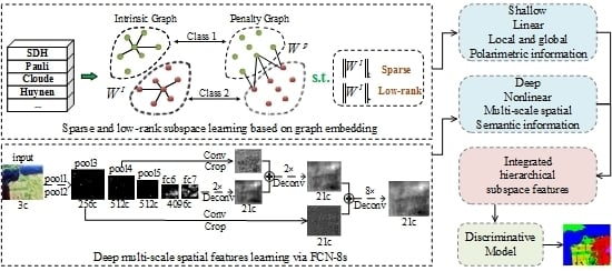
Figure 1.
The framework of the proposed methods. Upper left: learn sparse and low-rank subspace representations of high-dimensional polarimetric data. Lower left: learn deep multi-scale spatial features via FCN-8s. Middle column: visualizations of subspace features in 2D space and classification map. Right column: integrate hierarchical subspace features for classification combined with a discriminative model.

Figure 2.
Architectures of fully convolutional networks.

Figure 3.
The adjacency graphs of graph embedding.

Figure 4.
The flowchart of learning a low-dimensional sparse and low-rank subspace of high-dimensional PolSAR data based upon graph embedding. The features in the learned subspace are used for subsequent classification.
Figure 4.
The flowchart of learning a low-dimensional sparse and low-rank subspace of high-dimensional PolSAR data based upon graph embedding. The features in the learned subspace are used for subsequent classification.

Figure 5.
A simple illustration for receptive field of different layers. The receptive fields corresponding to location “A” and “B” are 9 and 36, respectively.
Figure 5.
A simple illustration for receptive field of different layers. The receptive fields corresponding to location “A” and “B” are 9 and 36, respectively.

Figure 6.
The procedure of extracting deep multi-scale spatial features via FCN-8s: “conv”, “Deconv” and “crop” denote convolutional operation, deconvolutional operation and crop operation, respectively. The 21D outputs of “score” layer are the desired deep spatial features.
Figure 6.
The procedure of extracting deep multi-scale spatial features via FCN-8s: “conv”, “Deconv” and “crop” denote convolutional operation, deconvolutional operation and crop operation, respectively. The 21D outputs of “score” layer are the desired deep spatial features.

Figure 7.
Visual feature maps in the first channel of specific layers of FCN-8s corresponding to Figure 6. (a) grayscale image of input layer; (b) pool1 layer; (c) pool2 layer; (d) pool3 layer; (e) pool4 layer; (f) pool5 layer; (g) fc6 layer; (h) fc7 layer; (i) score_fr layer; (j) upscore2 layer; (k) score_pool4c layer; (l) fuse_pool4 layer; (m) upscore_pool4 layer; (n) score_pool3c layer; (o) fuse_pool3 layer; (p) score layer.

Figure 8.
Visualizations of feature in 2D space by using t-SNE. Each sample is visualized as a point and samples with the same color belong to the same class. (a) raw polarimetric feature; (b) sparse and low-rank subspace feature; (c) deep spatial feature; (d) integrated hierarchical subspace feature.

Figure 9.
Flevoland dataset. (a) Pauli RGB; (b) ground truth and corresponding legend (note that the number of each class is given in brackets).
Figure 9.
Flevoland dataset. (a) Pauli RGB; (b) ground truth and corresponding legend (note that the number of each class is given in brackets).

Figure 10.
San Francisco dataset. (a) Pauli RGB; (b) ground truth and corresponding legend (note that the number of each class is given in brackets).
Figure 10.
San Francisco dataset. (a) Pauli RGB; (b) ground truth and corresponding legend (note that the number of each class is given in brackets).

Figure 11.
Flevoland Benchmark dataset. (a) Pauli RGB; (b) ground truth and corresponding legend (note that the number of each class is given in brackets).
Figure 11.
Flevoland Benchmark dataset. (a) Pauli RGB; (b) ground truth and corresponding legend (note that the number of each class is given in brackets).

Figure 12.
Overall accuracy versus reduced dimension using BSLGDA on three PolSAR data sets (with 1% training samples).
Figure 12.
Overall accuracy versus reduced dimension using BSLGDA on three PolSAR data sets (with 1% training samples).

Figure 13.
Overall accuracy versus different training samples ratios curves using BSLGDA+FCN on three PolSAR data sets (in their optimum dimensions). (a) Flevoland data set; (b) San Francisco data set; (c) Flevoland Benchmark data set.
Figure 13.
Overall accuracy versus different training samples ratios curves using BSLGDA+FCN on three PolSAR data sets (in their optimum dimensions). (a) Flevoland data set; (b) San Francisco data set; (c) Flevoland Benchmark data set.

Figure 14.
Classification confusion matrix for Flevoland data set by usingBSLGDA + FCN.

Figure 15.
Classification confusion matrix for San Francisco data set by using BSLGDA + FCN.

Figure 16.
Classification confusion matrix for Flevoland Benchmark data set by using BSLGDA + FCN.

Figure 17.
Classification maps resulting from the Flevoland data set with different algorithms. (a) BSLGDA: 73.77%; (b) FCN: 90.99%; (c) PCA + FCN: 81.97%.; (d) BLGDA + FCN: 95.78%; (e) BSGDA + FCN: 96.12%; (f) BSLGDA + FCN: 95.67%.
Figure 17.
Classification maps resulting from the Flevoland data set with different algorithms. (a) BSLGDA: 73.77%; (b) FCN: 90.99%; (c) PCA + FCN: 81.97%.; (d) BLGDA + FCN: 95.78%; (e) BSGDA + FCN: 96.12%; (f) BSLGDA + FCN: 95.67%.

Figure 18.
Classification maps resulting from the San Francisco data set with different algorithms. (a) BSLGDA: 86.51%; (b) FCN: 97.82%; (c) PCA + FCN: 94.70%; (d) BLGDA + FCN: 98.38%; (e) BSGDA + FCN: 98.04%; (f) BSLGDA + FCN: 98.34%.
Figure 18.
Classification maps resulting from the San Francisco data set with different algorithms. (a) BSLGDA: 86.51%; (b) FCN: 97.82%; (c) PCA + FCN: 94.70%; (d) BLGDA + FCN: 98.38%; (e) BSGDA + FCN: 98.04%; (f) BSLGDA + FCN: 98.34%.

Figure 19.
Classification maps resulting from the Flevoland Benchmark data set with different algorithms. (a) BSLGDA: 92.80%; (b) FCN: 97.45%; (c) PCA + FCN: 96.49%; (d) BLGDA + FCN: 99.71%; (e) BSGDA + FCN: 99.79%; (f) BSLGDA + FCN: 99.72%.
Figure 19.
Classification maps resulting from the Flevoland Benchmark data set with different algorithms. (a) BSLGDA: 92.80%; (b) FCN: 97.45%; (c) PCA + FCN: 96.49%; (d) BLGDA + FCN: 99.71%; (e) BSGDA + FCN: 99.79%; (f) BSLGDA + FCN: 99.72%.


Table 1.
SVM class-specific accuracy (%), OA and kappa coefficient of different methods for the Flevoland data set.
Table 1.
SVM class-specific accuracy (%), OA and kappa coefficient of different methods for the Flevoland data set.
| Class | BSLGDA | FCN | PCA + FCN | BLGDA + FCN | BSGDA + FCN | BSLGDA + FCN |
|---|---|---|---|---|---|---|
| 1 | 70.86 | 89.67 | 87.17 | 96.02 | 95.89 | 95.74 |
| 2 | 74.20 | 94.68 | 90.48 | 97.20 | 97.36 | 96.71 |
| 3 | 81.03 | 97.40 | 95.65 | 98.93 | 98.60 | 98.50 |
| 4 | 59.41 | 91.87 | 86.12 | 95.58 | 94.52 | 95.09 |
| 5 | 64.94 | 92.98 | 85.96 | 97.24 | 97.60 | 96.93 |
| 6 | 84.51 | 95.03 | 93.74 | 97.36 | 97.24 | 97.75 |
| 7 | 53.93 | 77.57 | 79.51 | 89.96 | 89.92 | 88.82 |
| 8 | 55.09 | 95.99 | 92.32 | 97.82 | 98.33 | 98.03 |
| 9 | 71.70 | 71.13 | 72.17 | 89.51 | 91.60 | 88.89 |
| 10 | 96.68 | 99.95 | 99.82 | 99.89 | 99.98 | 99.92 |
| 11 | 81.47 | 90.81 | 93.50 | 94.75 | 96.42 | 95.54 |
| OA | 73.77 | 90.99 | 81.97 | 95.78 | 96.12 | 95.67 |
| kappa | 0.7037 | 0.8982 | 0.7966 | 0.9524 | 0.9562 | 0.9512 |
Table 2.
SVM class-specific accuracy (%), OA and kappa coefficient of different methods for the San Francisco data set.
Table 2.
SVM class-specific accuracy (%), OA and kappa coefficient of different methods for the San Francisco data set.
| Class | BSLGDA | FCN | PCA + FCN | BLGDA + FCN | BSGDA + FCN | BSLGDA + FCN |
|---|---|---|---|---|---|---|
| 1 | 72.73 | 97.31 | 93.66 | 98.03 | 97.79 | 97.86 |
| 2 | 87.86 | 95.41 | 89.96 | 96.35 | 96.45 | 96.37 |
| 3 | 96.42 | 99.44 | 98.45 | 99.70 | 99.74 | 99.69 |
| 4 | 77.25 | 97.40 | 95.68 | 98.15 | 98.40 | 98.15 |
| 5 | 64.42 | 97.79 | 66.82 | 97.75 | 97.33 | 97.72 |
| OA | 86.51 | 97.82 | 94.70 | 98.38 | 98.04 | 98.34 |
| kappa | 0.8108 | 0.9693 | 0.9252 | 0.9772 | 0.9725 | 0.9767 |
Table 3.
SVM class-specific accuracy (%), OA and kappa coefficient of different methods for the Flevoland Benchmark data set.
Table 3.
SVM class-specific accuracy (%), OA and kappa coefficient of different methods for the Flevoland Benchmark data set.
| Class | BSLGDA | FCN | PCA + FCN | BLGDA + FCN | BSGDA + FCN | BSLGDA + FCN |
|---|---|---|---|---|---|---|
| 1 | 90.14 | 99.53 | 93.42 | 99.68 | 99.80 | 99.53 |
| 2 | 95.26 | 99.85 | 99.76 | 100 | 100 | 99.95 |
| 3 | 98.64 | 100 | 99.92 | 100 | 100 | 100 |
| 4 | 96.39 | 98.31 | 93.51 | 99.46 | 99.74 | 99.59 |
| 5 | 95.57 | 99.90 | 99.72 | 99.95 | 99.97 | 99.81 |
| 6 | 44.56 | 99.80 | 93.57 | 98.52 | 99.82 | 99.60 |
| 7 | 96.46 | 99.78 | 99.63 | 99.98 | 99.88 | 99.80 |
| 8 | 51.12 | 90.54 | 40.59 | 95.70 | 99.51 | 96.68 |
| 9 | 89.96 | 99.27 | 60.96 | 99.41 | 99.22 | 99.46 |
| 10 | 90.86 | 99.27 | 73.96 | 99.59 | 99.84 | 99.35 |
| 11 | 99.46 | 100 | 96.70 | 99.98 | 100 | 100 |
| 12 | 95.81 | 99.52 | 99.49 | 99.66 | 99.71 | 99.83 |
| 13 | 75.37 | 98.65 | 95.46 | 98.77 | 99.57 | 99.35 |
| 14 | 76.42 | 100 | 99.61 | 100 | 99.93 | 100 |
| OA | 92.80 | 97.45 | 96.49 | 99.71 | 99.79 | 99.72 |
| kappa | 0.9153 | 0.9653 | 0.9587 | 0.9966 | 0.9975 | 0.9967 |
Table 4.
Execution time (in seconds) of extracting features via FCN-8s for the three experimental data sets.
Table 4.
Execution time (in seconds) of extracting features via FCN-8s for the three experimental data sets.
| Dataset | Flevoland | San Francisco | Flevoland Benchmark |
|---|---|---|---|
| Pixels | 750 × 1024 | 900 × 1024 | 1020 × 1024 |
| Time | 60.44 | 70.14 | 79.98 |
Table 5.
Execution time (in seconds) of classification in the three experimental data sets.
| Dataset | BSLGDA | FCN | PCA + FCN | BLGDA + FCN | BSGDA + FCN | BSLGDA + FCN |
|---|---|---|---|---|---|---|
| Flevoland | 183.96 | 14.37 | 15.78 | 196.04 | 3060.93 | 169.71 |
| San Francisco | 1390.89 | 13.99 | 16.23 | 1270.10 | 4980.51 | 1849.22 |
| Flevoland Benchmark | 27.69 | 11.83 | 12.39 | 28.60 | 506.56 | 29.22 |
© 2018 by the authors. Licensee MDPI, Basel, Switzerland. This article is an open access article distributed under the terms and conditions of the Creative Commons Attribution (CC BY) license (http://creativecommons.org/licenses/by/4.0/).
Share and Cite
MDPI and ACS Style
Wang, Y.; He, C.; Liu, X.; Liao, M. A Hierarchical Fully Convolutional Network Integrated with Sparse and Low-Rank Subspace Representations for PolSAR Imagery Classification. Remote Sens. 2018, 10, 342. https://doi.org/10.3390/rs10020342
AMA Style
Wang Y, He C, Liu X, Liao M. A Hierarchical Fully Convolutional Network Integrated with Sparse and Low-Rank Subspace Representations for PolSAR Imagery Classification. Remote Sensing. 2018; 10(2):342. https://doi.org/10.3390/rs10020342
Chicago/Turabian StyleWang, Yan, Chu He, Xinlong Liu, and Mingsheng Liao. 2018. "A Hierarchical Fully Convolutional Network Integrated with Sparse and Low-Rank Subspace Representations for PolSAR Imagery Classification" Remote Sensing 10, no. 2: 342. https://doi.org/10.3390/rs10020342
Note that from the first issue of 2016, this journal uses article numbers instead of page numbers. See further details here.