Progressive Sample Processing of Band Selection for Hyperspectral Image Transmission


Abstract
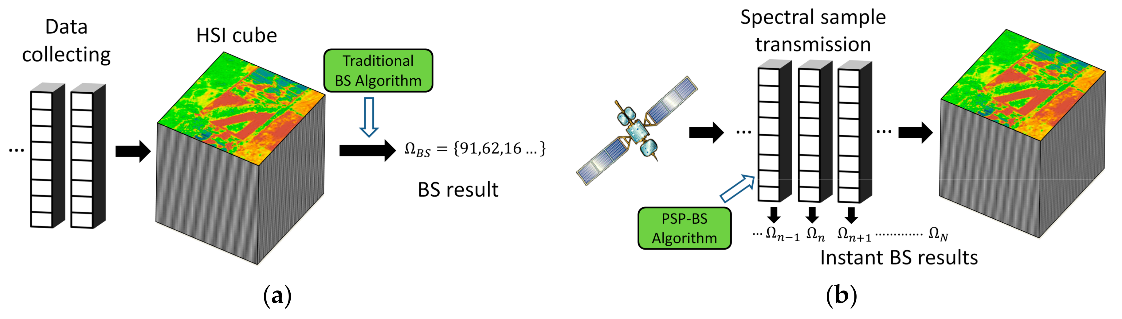
:1. Introduction
2. Orthogonal Matching Pursuit-Based BS (OMPBS)
| Algorithm 1. OMPBS |
| Objective: Find p representative bands for a HSI cube |
| Input: ( matrix), sparsity = |
| Output: Band indices set |
| Steps: |
| 1. Initialization: Set , , , . |
| 2. At j-th iteration, calculate the row norm vector of matrix . |
| 3. Find the row index whose value is maximum at . Then set , . |
| 4. Solve the sub optimization problem by . |
| 5. Update the residual matrix . |
| 6. If , break; otherwise, set and go to Step 2. |
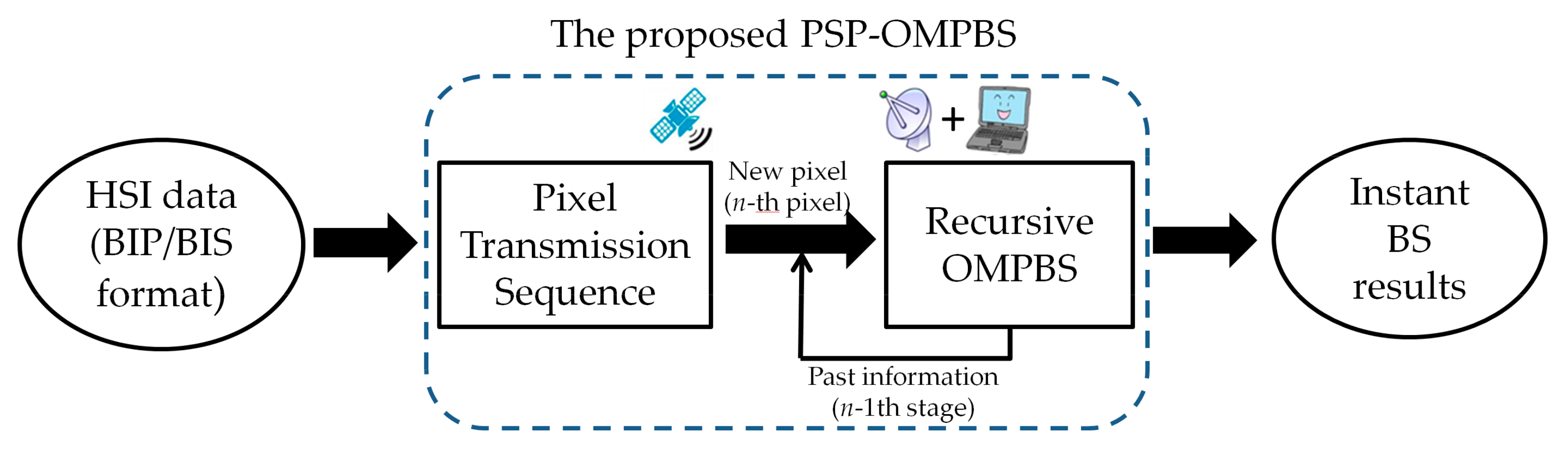
3. Progressive Sample Processing-Based OMPBS (PSP-OMPBS)
3.1. Derivation of Recursive OMPBS (Re-OMPBS)
3.1.1. Decomposition of the Least Square Estimator
3.1.2. Decomposition of the Residual Multiplication Term
3.2. Condition for Applying Recursive Equations
3.3. Re-OMPBS Algorithm
| Algorithm 2. Re-OMPBS |
| Objective: Find the BS of the nth stage during BIP/BIS transmission |
| Input: |
| 2. Processed information: • Previous BS result: • Previous sparse coefficient matrices: • Previous auxiliary matrix: • Other terms and |
| 3. New information: n-th pixel: |
| Output: Band indices |
| Steps: |
| 1. Initialization: Set , , j=1, . |
| 2. At the jth iteration, calculate the vector-wise norms of all rows in matrix , and denote it by column vector , . |
| 3. Find the row index whose value is maximum is k, denoted by . Then set , . |
| 4. If , using Equation (9) to calculate ; otherwise, . |
| 5. Update auxiliary matrix by equation . |
| 6. Update the residual term by Equations (11)–(14). |
| 7. If , break; otherwise, and go to Step 2. |
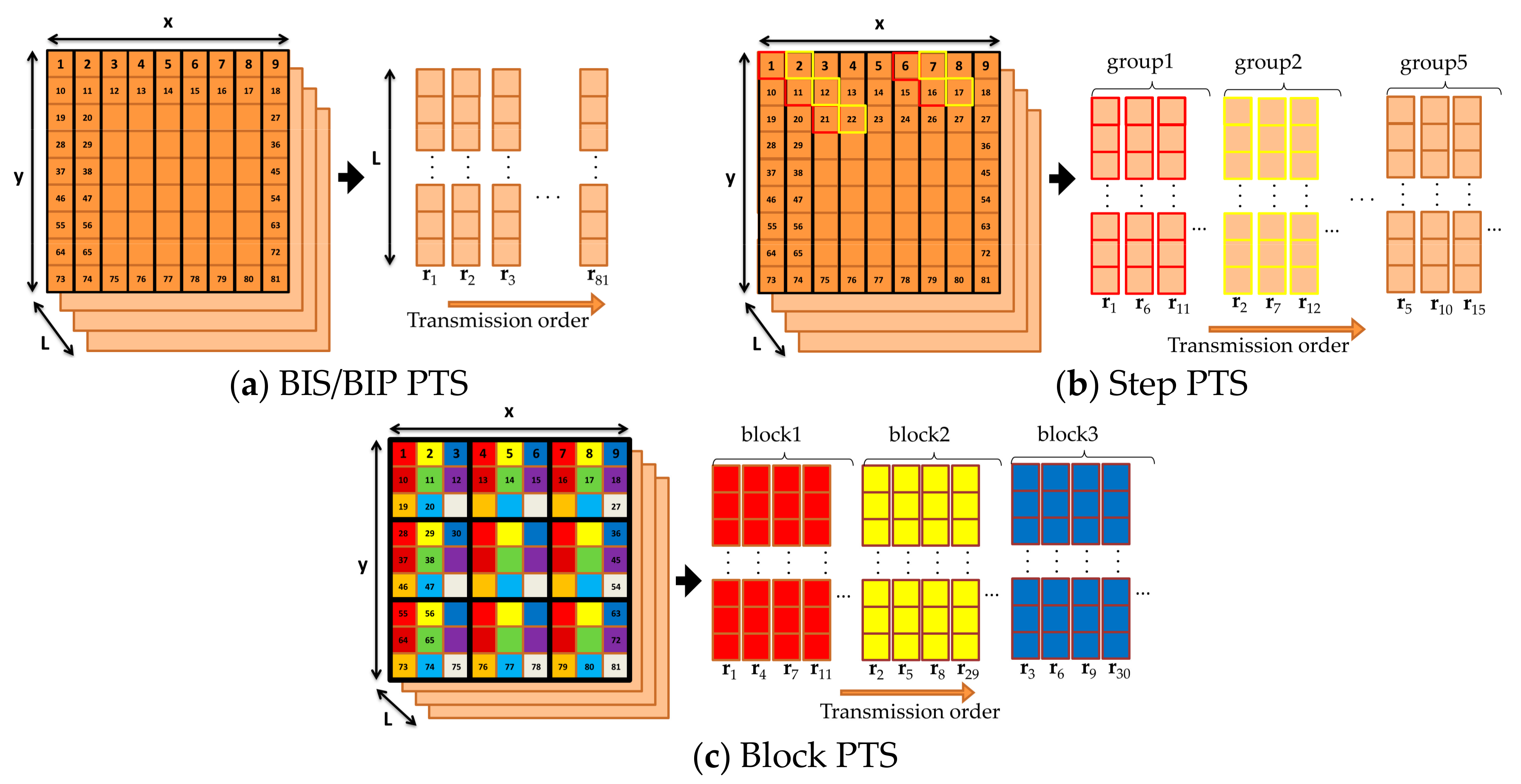
3.4. Design of Pixel Transmission Sequence (PTS)
3.4.1. Original Band-Interleaved-by-Sample/Pixel (BIS/BIP) Sequence
3.4.2. Step Sequence
3.4.3. Block Sequence
4. Experiments
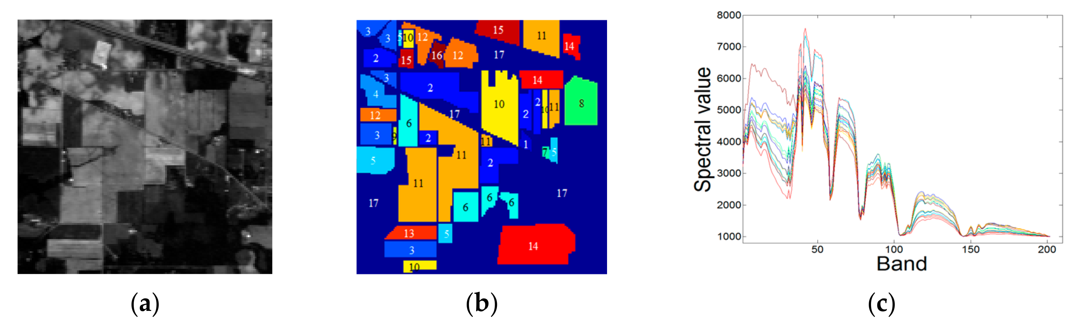
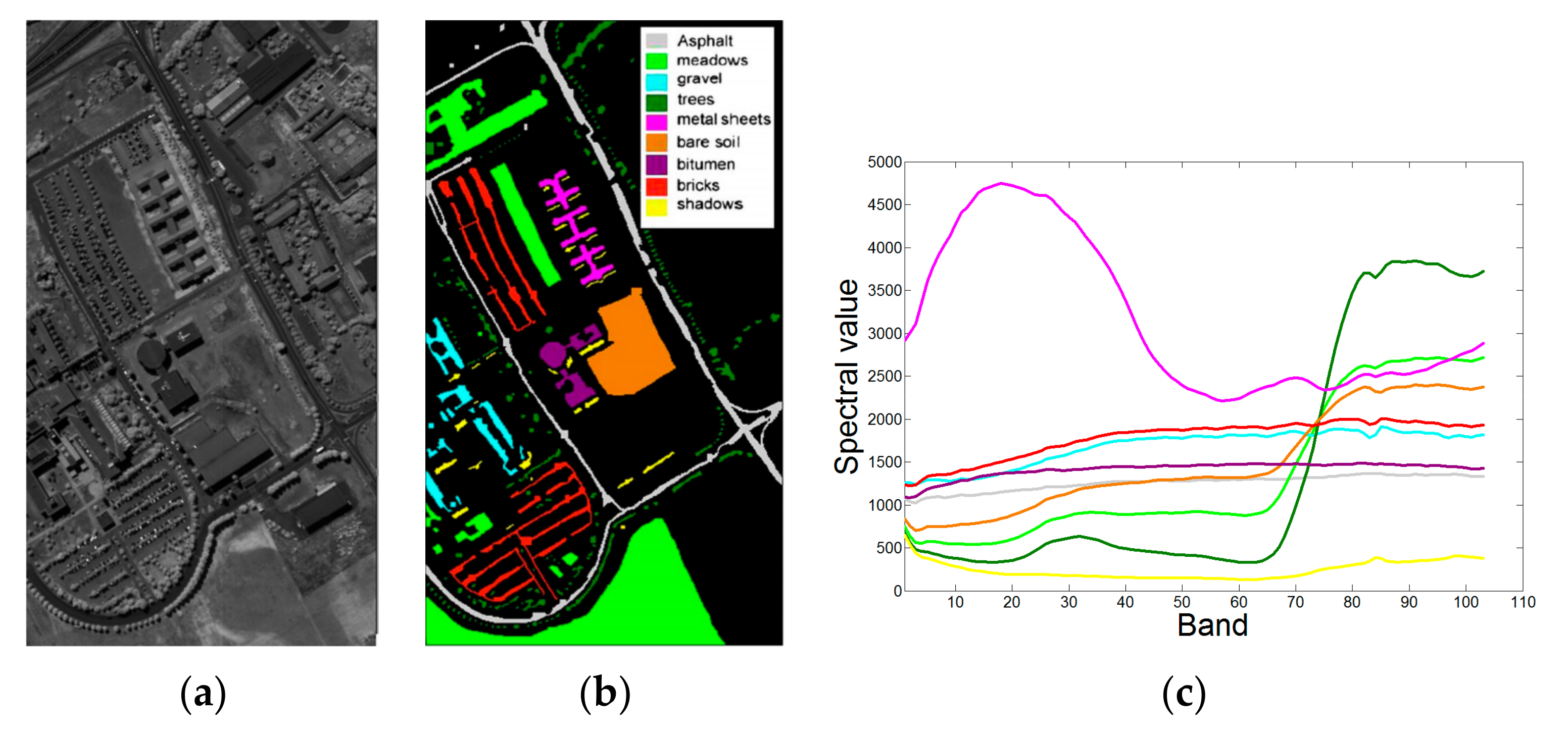
4.1. Hyperspectral Dataset and Experimental Setting
4.2. BS Accuracy Analysis
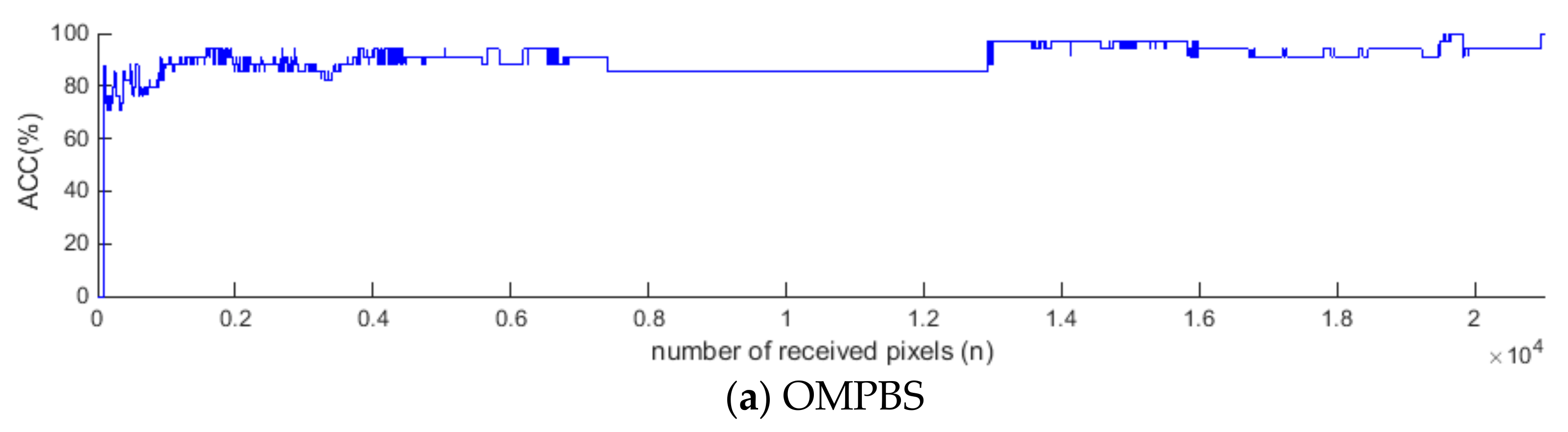
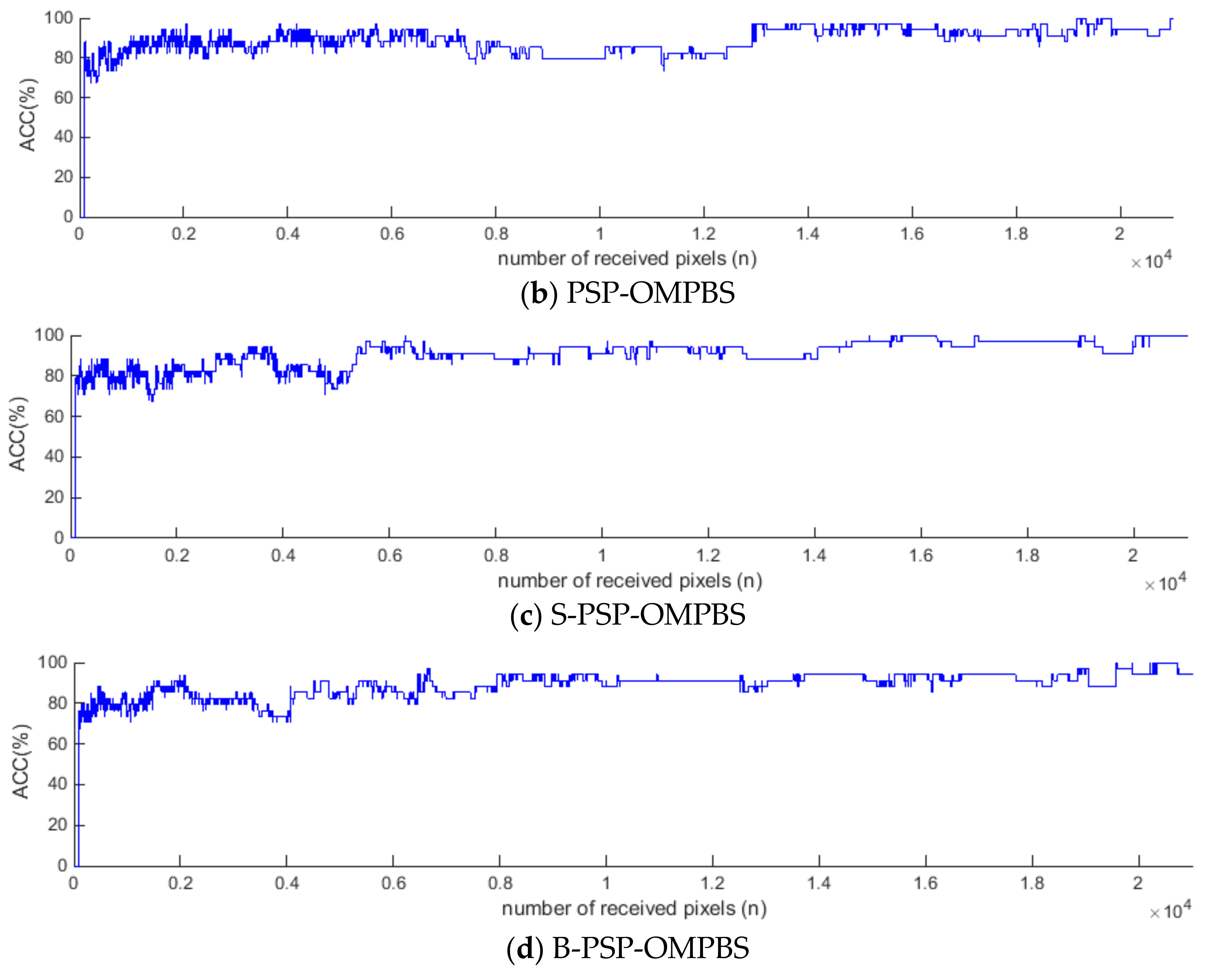
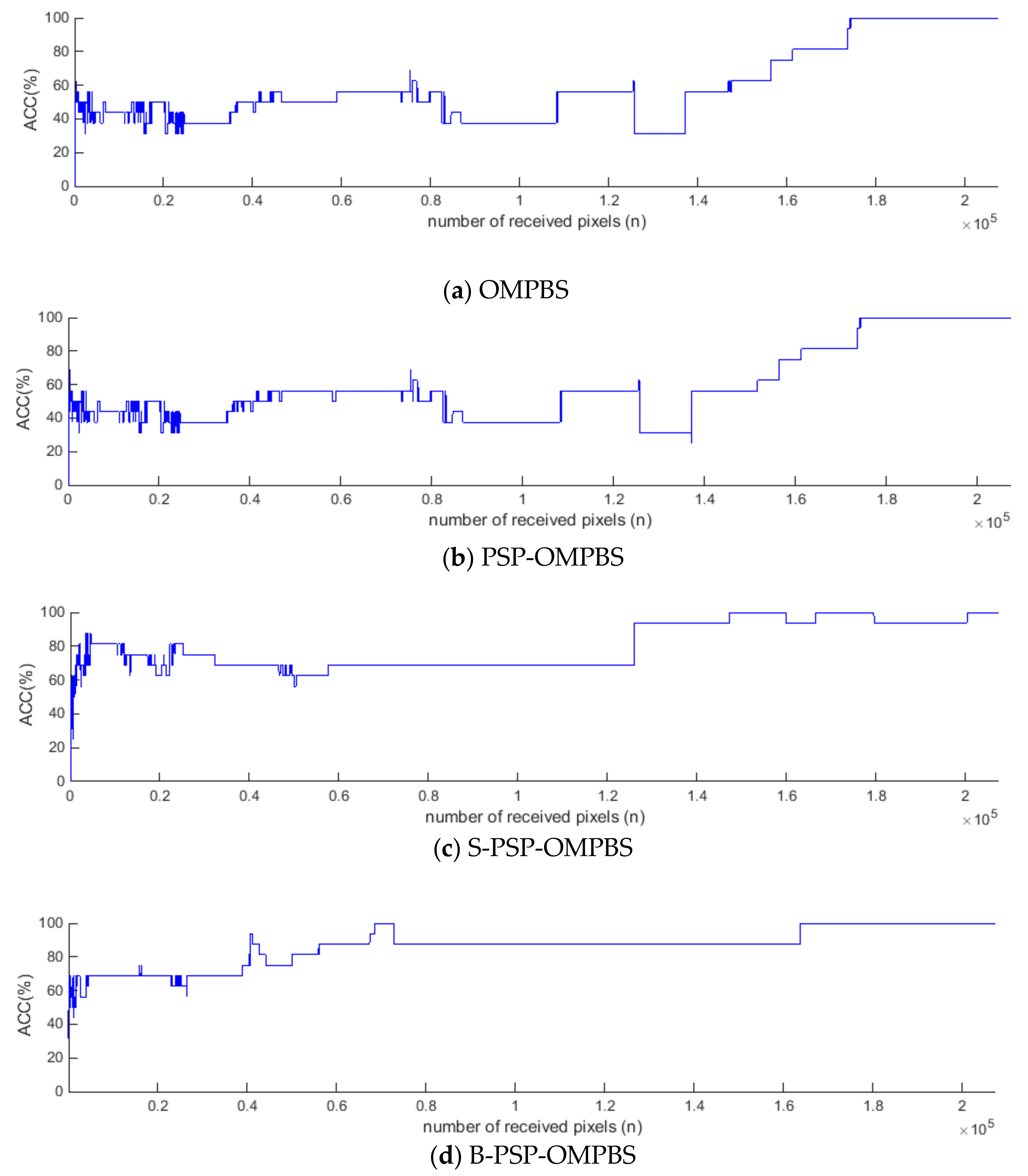
- Comparing Figure 6a with Figure 6b, the tendency of the ACC curves of OMPBS and PSP-OMPBS are nearly the same. This implies that the derivation of Re-OMPBS is correct. In fact, these two curves are still slightly different in some regions. Based on our study, the difference was caused by the numerical errors produced by using the recursive equations derived from Woodbury’s Identity.
- In the OMPBS and PSP-OMPBS curves, the ACC values kept at 40~60% when n is less than 1.5 × 10⁵. This is mainly due to the fact that these values were generated by using the original BIS/BIP PTS. The BS results could not stabilize quickly.
- The ACC results of using step sequence are shown in Figure 6c. We find that the ACC values located between 60~80% at n [2000,125,000]. After receiving 1.25 × 105 pixels, the ACCs increased to 90%. In other words, using the PTS formed by uniform sampling drastically accelerated the speed of convergence. It suggests that using full pixels is not necessary to obtain the correct BS result using PSP-OMPBS. The nearly-correct BS result could be obtained during transmission.
- Using a block pixel transmission sequence also accelerated the BS convergence. Figure 6d shows the corresponding ACC results of B-PSP-OMPBS. Similar conclusions can be drawn. It only requires 40,000 pixels to reach 65–70% accuracy. After receiving 60,000 pixels, the ACC grew to over 80%. The overall ACC performance is undoubtedly better than OMPBS, PSP-OMPBS, and even S-PSP-OMPBS.
- In Figure 6a–d , it can be seen that the ACC curves remain flat in some segments. In those regions, the BS results kept the same. That is, the new incoming pixels did not change the BS results.
- All the curves reached 100% at n = N = 207,400.
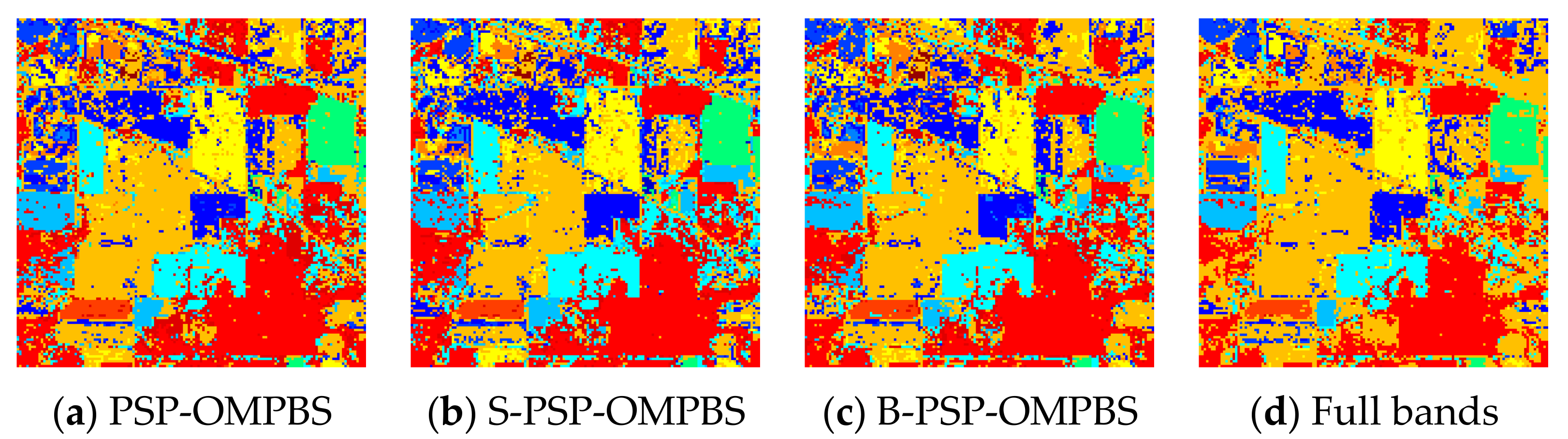
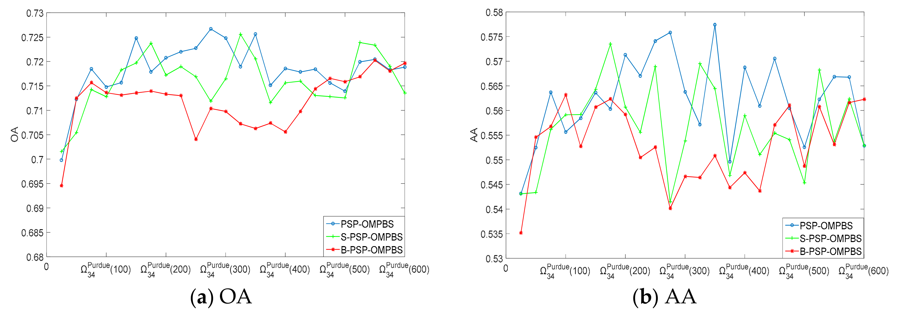
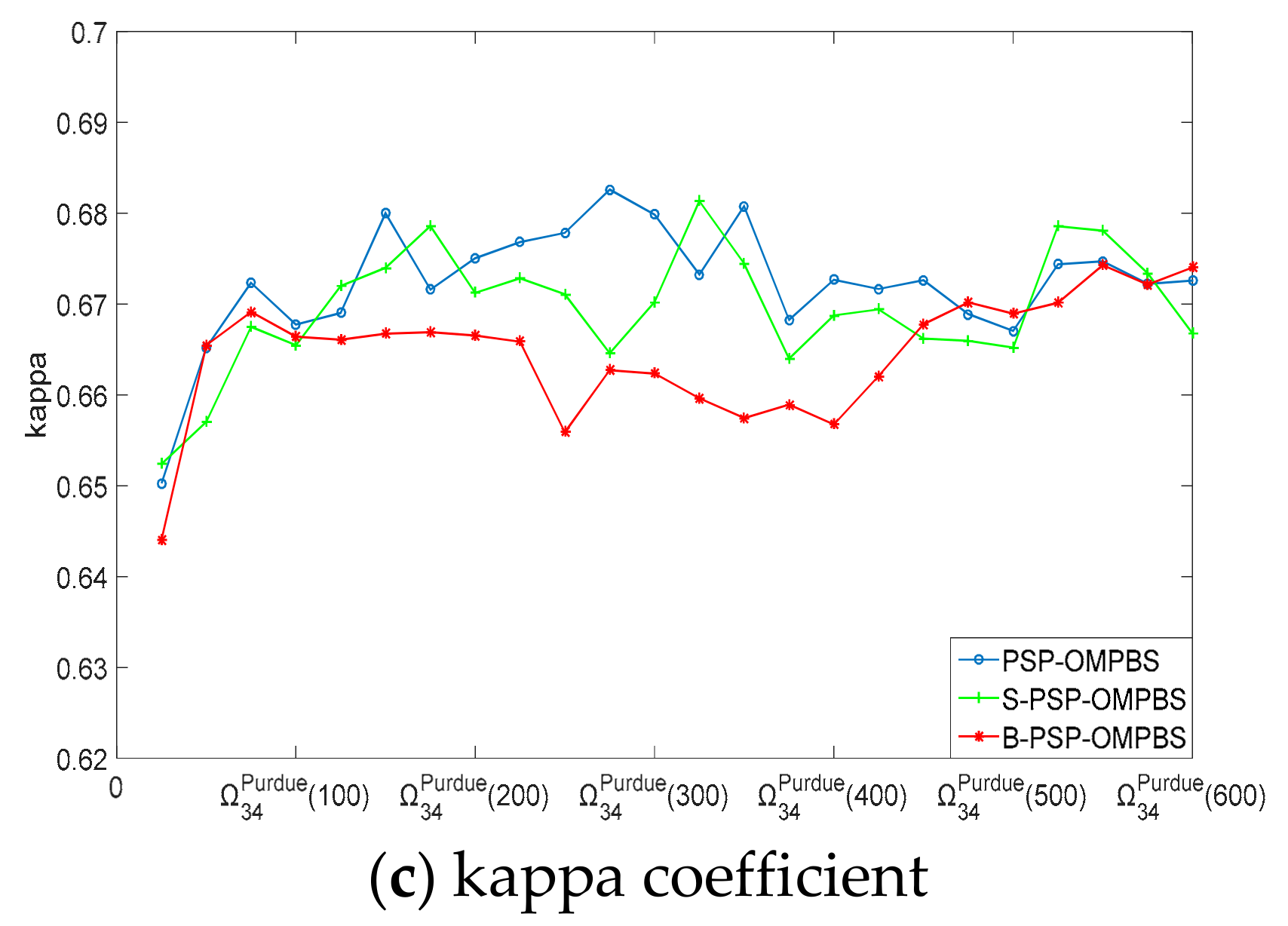
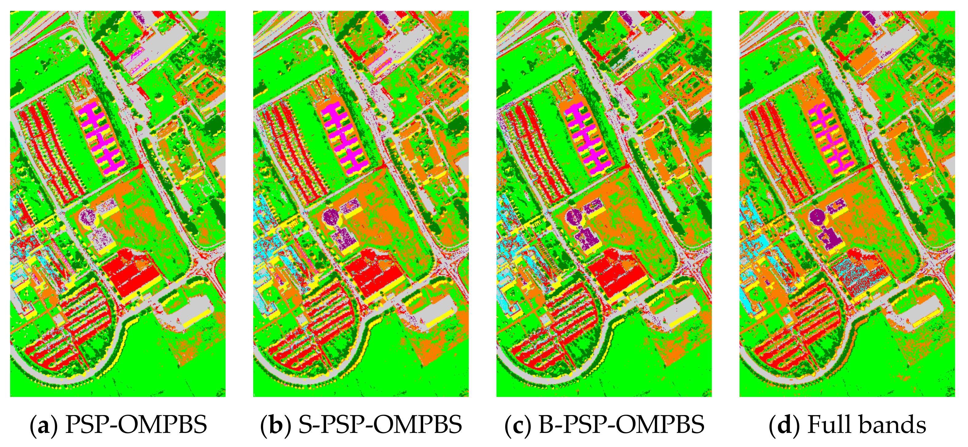
4.3. Land Cover Classification
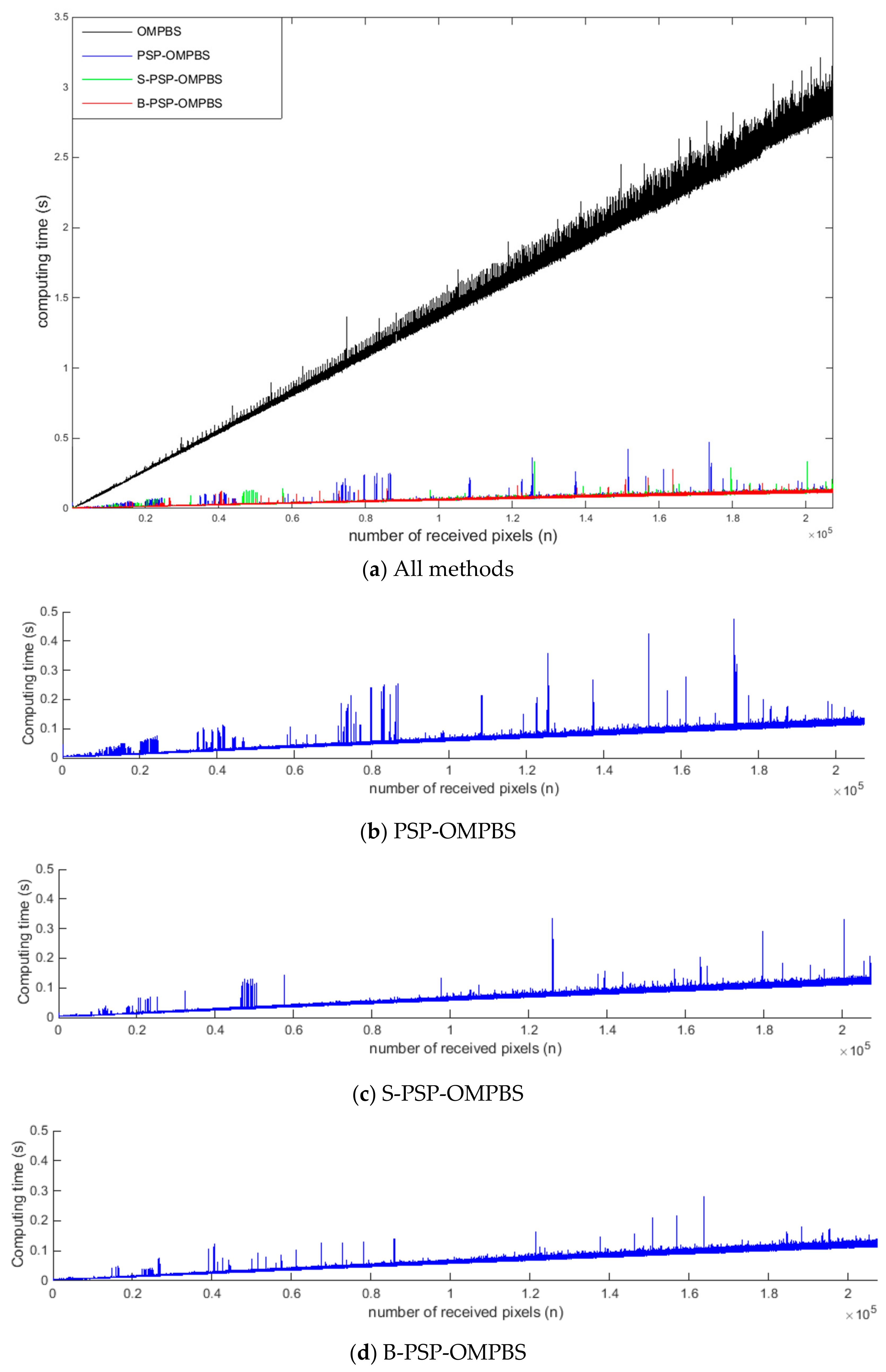
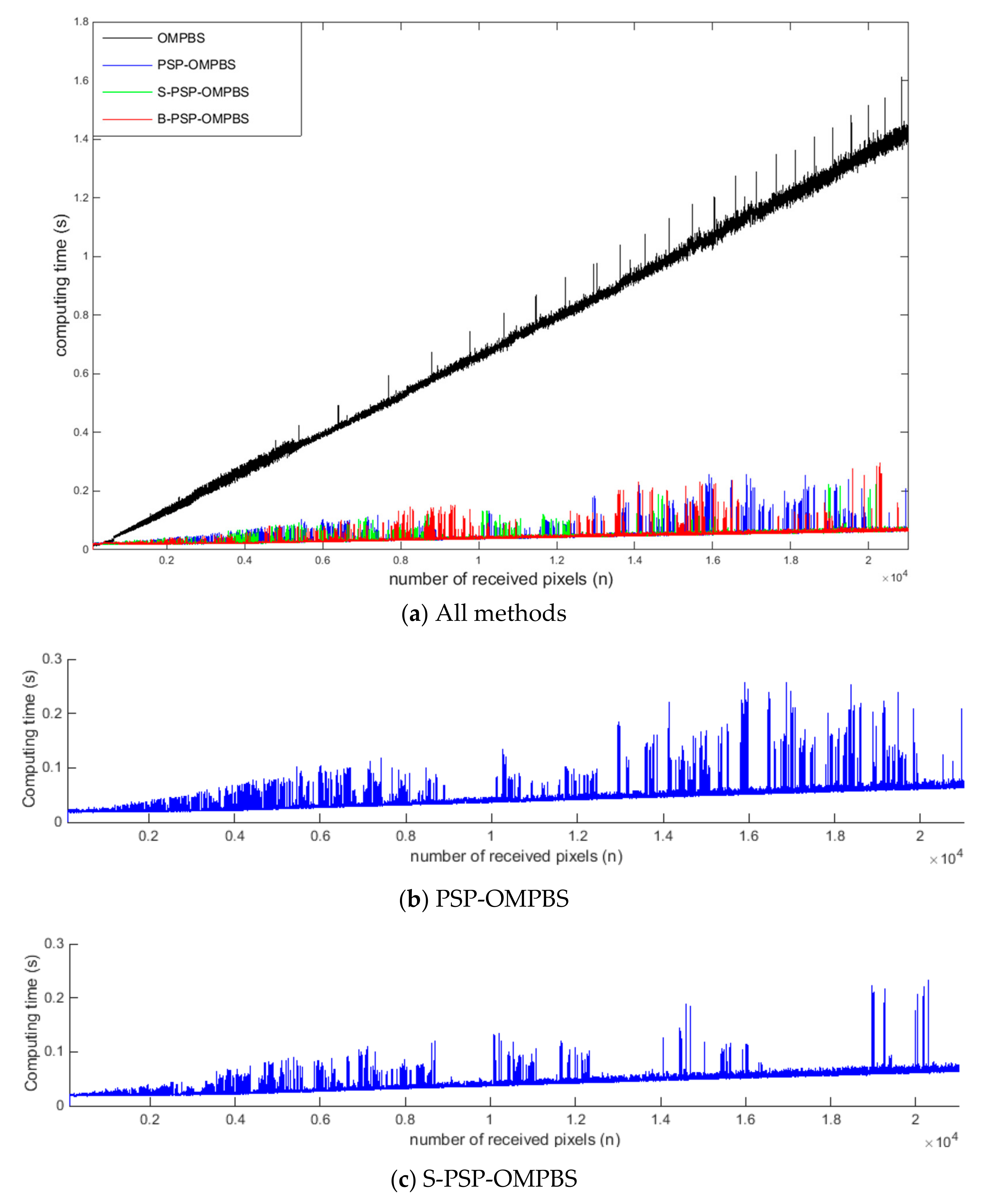
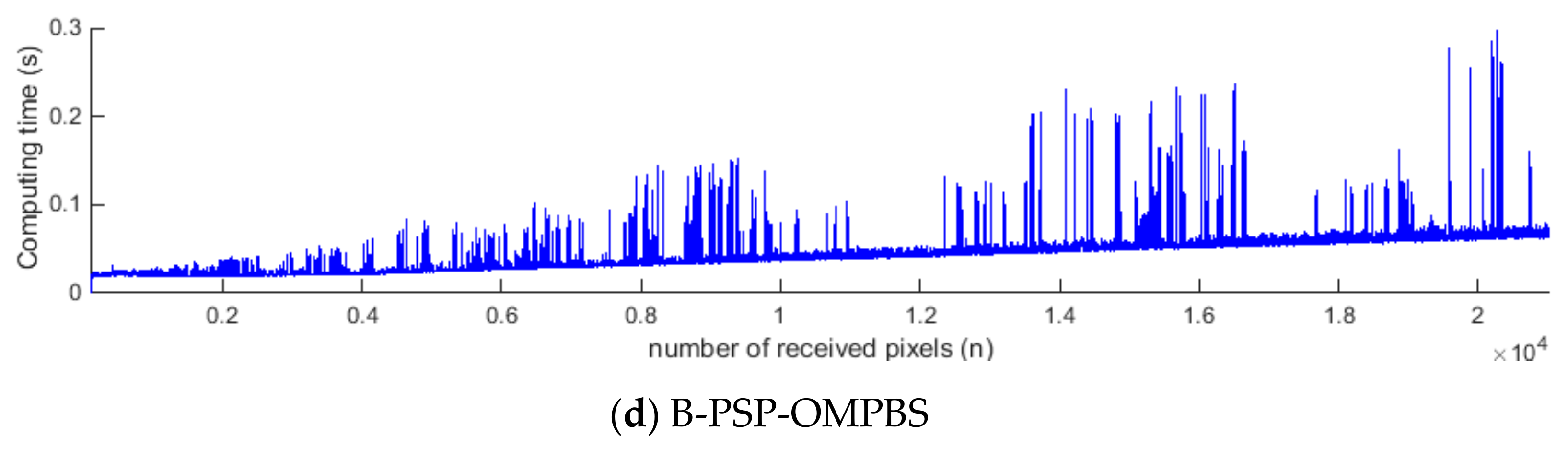
4.4. Computing Time
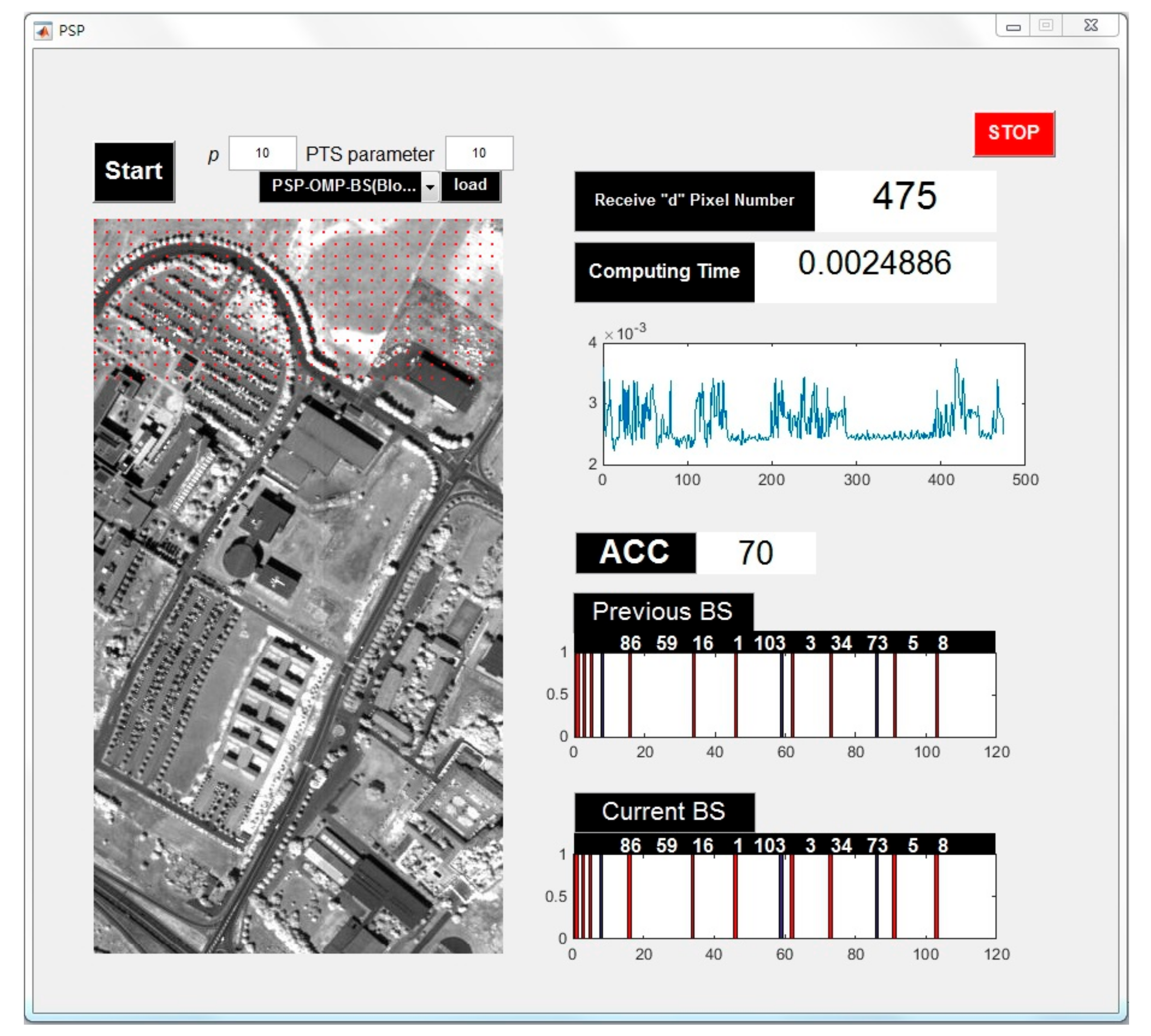
4.5. Graphical User Intervace Design
5. Discussion
6. Conclusions
Acknowledgments
Author Contributions
Conflicts of Interest
References
- Maisel, P.W.; Kramber, W.J.; Lee, J.K. Optimum band selection for supervised classification of multispectral data. Photogramm. Eng. Remote Sens. 1990, 56, 55–60. [Google Scholar]
- Keshava, N. Distance metrics and band selection in hyperspectral processing with applications to material identification and spectral libraries. IEEE Trans. Geosci. Remote Sens. 2004, 42, 1552–1565. [Google Scholar] [CrossRef]
- Du, Q.; Yang, H. Similarity-based unsupervised band selection for Hyperspectral Image Analysis. IEEE Geosci. Remote Sens. Lett. 2008, 5, 564–568. [Google Scholar] [CrossRef]
- Chang, C.-I.; Wang, S. Constrained band selection for hyperspectral imagery. IEEE Trans. Geosci. Remote Sens. 2006, 44, 1575–1585. [Google Scholar] [CrossRef]
- Martínez-Usó, A.; Pla, F.; Sotoca, J.M.; García-Sevilla, P. Clustering-Based Hyperspectral Band Selection Using Information Measures. IEEE Trans. Geosci. Remote Sens. 2007, 45, 4158–4171. [Google Scholar] [CrossRef]
- Guo, B.; Gunn, S.; Damper, B.; Nelson, J. Adaptive band selection for hyperspectral image fusion using mutual information. In Proceedings of the 8th IEEE International Conference on Information Fusion, Philadelphia, PA, USA, 25–28 July 2005; p. 8. [Google Scholar]
- Feng, J.; Jiao, L.C.; Zhang, X.; Sun, T. Hyperspectral Band Selection Based on Trivariate Mutual Information and Clonal Selection. IEEE Trans. Geosci. Remote Sens. 2014, 52, 4092–4105. [Google Scholar] [CrossRef]
- Feng, J.; Jiao, L.; Liu, F.; Sun, T.; Zhang, X. Mutual-Information-Based Semi-Supervised Hyperspectral Band Selection With High Discrimination, High Information, and Low Redundancy. IEEE Trans. Geosci. Remote Sens. 2015, 53, 2956–2969. [Google Scholar] [CrossRef]
- Sun, W.; Zhang, L.; Du, B. A Sparse Self-Representation Method for Band Selection in Hyperspectral Imagery Classification. In Proceedings of the 7th IEEE Workshop on Hyperspectral Image and Signal Processing: Evolution in Remote Sensing (Whispers), Tokyo, Japan, 2–5 June 2015; IEEE: New York, NY, USA; pp. 1–4. [Google Scholar]
- Sun, W.; Zhang, L.; Zhang, L.; Lai, Y.M. A Dissimilarity-Weighted Sparse Self-Representation Method for Band Selection in Hyperspectral Imagery Classification. IEEE J. Sel. Top. Appl. Earth Obs. Remote Sens. 2016, 9, 4374–4388. [Google Scholar] [CrossRef]
- Sun, W.; Jiang, M.; Li, W.; Liu, Y. A Symmetric Sparse Representation Based Band Selection Method for Hyperspectral Imagery Classification. Remote Sens. 2016, 8, 238. [Google Scholar] [CrossRef]
- Lai, C.H.; Chen, C.S.; Chen, S.Y.; Liu, K.H. Sequential band selection method based on orthogonal matching pursuit. In Proceedings of the 8th IEEE Workshop on Hyperspectral Image and Signal Processing: Evolution in Remote Sensing (WHISPERS), Los Angeles, CA, USA, 21–24 August 2016; IEEE: New York, NY, USA; pp. 1–4. [Google Scholar]
- Fisher, K.; Chang, C.-I. Progressive band selection for satellite hyperspectral data compression and transmission. J. Appl. Remote Sens. 2010, 4, 041770. [Google Scholar]
- Chang, C.-I.; Liu, K.-H. Progressive Band Selection of Spectral Unmixing for Hyperspectral Imagery. IEEE Trans. Geosci. Remote Sens. 2014, 52, 2002–2017. [Google Scholar] [CrossRef]
- Liu, S.; Du, Q.; Tong, X.; Samat, A.; Pan, H.; Ma, X. Band Selection-Based Dimensionality Reduction for Change Detection in Multi-Temporal Hyperspectral Images. Remote Sens. 2017, 9, 1008. [Google Scholar] [CrossRef]
- Geng, X.; Sun, K.; Ji, L.; Zhao, Y. A Fast Volume-Gradient-Based Band Selection Method for Hyperspectral Image. IEEE Trans. Geosci. Remote Sens. 2014, 52, 7111–7119. [Google Scholar] [CrossRef]
- Iordache, M.D.; Bioucas-Dias, J.M.; Plaza, A. Potential and limitations of band selection and library pruning in sparse hyperspectral unmixing. Proceedings of 2015 7th Workshop on Hyperspectral Image and Signal Processing: Evolution in Remote Sensing (WHISPERS), Tokyo, Japan, 2–5 June 2015; IEEE: New York, NY, USA; pp. 1–4. [Google Scholar]
- Chang, Y.L.; Chang, L.; Fang, J.P. Particle swarm optimization/impurity function class overlapping scheme based on multiple attribute decision making model for hyperspectral band selection. Proceedings of 2015 IEEE International CONFERENCE Geoscience and Remote Sensing Symposium (IGARSS), Milan, Italy, 26–31 July 2015; IEEE: New York, NY, USA; pp. 441–444. [Google Scholar]
- Huber-Lerner, M.; Hadar, O.; Rotman, S.R.; Huber-Shalem, R. Hyperspectral Band Selection for Anomaly Detection: The Role of Data Gaussianity. IEEE J. Sel. Top. Appl. Earth Obs. Remote Sens. 2016, 9, 732–743. [Google Scholar] [CrossRef]
- Cao, X.; Xiong, T.; Jiao, L. Supervised Band Selection Using Local Spatial Information for Hyperspectral Image. IEEE Geosci. Remote Sens. Lett. 2016, 13, 329–333. [Google Scholar] [CrossRef]
- Zhan, Y.; Hu, D.; Xing, H. Hyperspectral Band Selection Based on Deep Convolutional Neural Network and Distance Density. IEEE Geosci. Remote Sens. Lett. 2017, 14, 2365–2369. [Google Scholar] [CrossRef]
- Wang, L.; Li, H.C.; Xue, B.; Chang, C.I. Constrained Band Subset Selection for Hyperspectral Imagery. IEEE Geosci. Remote Sens. Lett. 2017, 14, 2032–2036. [Google Scholar] [CrossRef]
- Zhu, G.; Huang, Y.; Li, S.; Tang, J.; Liang, D. Hyperspectral Band Selection via Rank Minimization. IEEE Geosci. Remote Sens. Lett. 2017, 14, 2320–2324. [Google Scholar] [CrossRef]
- Park, H.; Choi, J.; Park, N.; Choi, S. Sharpening the VNIR and SWIR Bands of Sentinel-2A Imagery through Modified Selected and Synthesized Band Schemes. Remote Sens. 2017, 9, 1080. [Google Scholar] [CrossRef]
- Yang, C.; Tan, Y.; Bruzzone, L.; Lu, L. Discriminative Feature Metric Learning in the Affinity Propagation Model for Band Selection in Hyperspectral Images. Remote Sens. 2017, 9, 782. [Google Scholar] [CrossRef]
- Hihara, H.; Moritani, K.; Inoue, M.; Hoshi, Y.; Iwasaki, A.; Takada, J.; Inada, H.; Suzuki, M.; Seki, T.; Ichikawa, S.; Tanii, J. On board Image Processing System for Hyperspectral Sensor. Sensors 2015, 15, 24926–24944. [Google Scholar] [CrossRef] [PubMed]
- Conoscenti, M.; Coppola, R.; Magli, E. Constant SNR, Rate Control, and Entropy Coding for Predictive Lossy Hyperspectral Image Compression. IEEE Trans. Geosci. Remote Sens. 2016, 54, 7431–7441. [Google Scholar] [CrossRef]
- Giordano, R.; Lombardi, A.; Guccione, P. Efficient clustering and on-board ROI-based compression for Hyperspectral Radar. In Proceedings of the IARIA Conference, Lisbon, Portugal, 26–30 June 2016; pp. 33–38. [Google Scholar]
- Giordano, R.; Guccione, P. ROI-Based On-Board Compression for Hyperspectral Remote Sensing Images on GPU. Sensors 2017, 17, 1160. [Google Scholar] [CrossRef] [PubMed]
- Quesada-Barriuso, P.; Argüello, F.; Heras, D.B. Computing Efficiently Spectral-Spatial Classification of Hyperspectral Images on Commodity GPUs. In Recent Advances in Knowledge-based Paradigms and Applications. Advances in Intelligent Systems and Computing; Springer: Cham, Switzerland, 2014. [Google Scholar]
- Ma, N.; Wang, S.; Ali, S.M.; Cui, X.; Peng, Y. High Efficiency On-Board Hyperspectral Image Classification with Zynq SoC. Proceedings of 2016 7th International Conference on Mechatronics and Manufacturing (ICMM 2016), Harbin, China, 16 March 2016; Volume 45. [Google Scholar] [CrossRef]
- Chang, C.I. Overview and Introduction. In Real-Time Progressive Hyperspectral Image Processing; Springer-Verlag: New York, NY, USA, 2016; pp. 1–32. [Google Scholar]
- Chang, C.I.; Wu, C.C.; Liu, K.H.; Chen, H.M.; Chen, C.C.C.; Wen, C.H. Progressive Band Processing of Linear Spectral Unmixing for Hyperspectral Imagery. IEEE J. Sel. Top. Appl. Earth Obs. Remote Sens. 2015, 8, 2583–2597. [Google Scholar] [CrossRef]
- Chang, C.I.; Li, Y.; Hobbs, M.C.; Schultz, R.C.; Liu, W.M. Progressive Band Processing of Anomaly Detection in Hyperspectral Imagery. IEEE J. Sel. Top. Appl. Earth Obs. Remote Sens. 2015, 8, 3558–3571. [Google Scholar] [CrossRef]
- Chang, C.I.; Schultz, R.C.; Hobbs, M.C.; Chen, S.Y.; Wang, Y.; Liu, C. Progressive Band Processing of Constrained Energy Minimization for Subpixel Detection. IEEE Trans. Geosci. Remote Sens. 2015, 53, 1626–1637. [Google Scholar] [CrossRef]
- Elhamifar, E.; Sapiro, G.; Vidal, R. See all by looking at a few: Sparse modeling for finding representative objects. Proceedings of IEEE Conference on Computer Vision and Pattern Recognition (CVPR), Providence, RI, USA, 16–21 June 2012; IEEE: New York, NY, USA; pp. 1600–1607. [Google Scholar]
- Tropp, J.A.; Gilbert, A.C. Signal Recovery from Random Measurements via Orthogonal Matching Pursuit. IEEE Trans. Inf. Theory 2007, 53, 4655–4666. [Google Scholar] [CrossRef]
- Woodbury Matrix Identity. Available online: https://en.wikipedia.org/wiki/Woodbury_matrix_identity (accessed on 10 December 2017).
- Chang, C.-I.; Du, Q. Estimation of number of spectrally distinct signal sources in hyperspectral imagery. IEEE Trans. Geosci. Remote Sens. 2004, 42, 608–619. [Google Scholar] [CrossRef]
- LibSVM. Available online: https://www.csie.ntu.edu.tw/~cjlin/libsvm/ (accessed on 18 January 2018).


| OMPBS | PSP-OMPBS (proposed) | |
|---|---|---|
| Description | A traditional BS method which is implemented on a pre-obtained image data. | A PSP-BS method. It is used in the moment of spectral sample transmission or collecting. |
| Core algorithm | OMP-BS [37] | Re-OMPBS (Algorithm 2) |
| Use of past information | No | Yes |
| Use of PTS | No | Yes (Original/Step/Block) |
| Least square estimator used in the optimization | Recursive Equation (9) | |
| Residual term calculation | Direct computation | Recursive Equations (11)–(14) |
| Capable for progressive processing | No, the computing time will increase with the data volume. | Yes |
| Parameter | Pavia Data | Purdue Data |
|---|---|---|
| N (number of total pixel) | 207,400 | 21,025 |
| p (number of selected bands) | 16 | 34 |
| k (step size of step PTS) | 200 | 100 |
| b (block size of block PTS) | 50 | 25 |
| Method | Selected Bands | ACC |
|---|---|---|
| OMPBS | 86,20,63,1,103,3,45,73,6,32,83,9,4,55,12,2 | 37.5 |
| PSP-OMPBS | 86,20,63,1,103,3,45,73,6,32,83,9,4,55,12,2 | 37.5 |
| S-PSP-OMPBS | 91,62,15,1,33,3,73,103,5,46,85,7,2,83,10,22 | 68.75 |
| B-PSP-OMPBS | 91,62,16,1,34,3,73,103,5,47,46,48,85,8,83,2 | 87.5 |
| OMPBS (full pixels) | 91,62,16,1,34,3,73,103,5,46,85,8,83,2,11,78 | N/A |
| Method | Selected Bands | ACC |
|---|---|---|
| OMPBS | 42,29,2,89,6,35,1,53,117,3,4,15,38,5,32,72,41,104,7,39,34,8,37,43,9,44,97,63,45,10,33,36,46,40 | 85.31 |
| PSP-OMPBS | 42,29,2,89,6,35,1,53,117,3,4,15,16,38,5,32,72,41,104,7,39,34,8,37,43,44,45,97,9,63,33,10,46,36 | 85.29 |
| S-PSP-OMPBS | 42,29,3,89,35,1,2,70,9,118,4,38,5,32,14,44,16,6,144,43,39,97,34,7,45,37,63,8,41,48,52,47,50,10 | 88.24 |
| B-PSP-OMPBS | 42,29,2,89,35,6,1,70,118,3,38,4,14,5,32,43,144,44,7,39,34,97,8,45,11,48,37,63,41,100,46,9,33,17 | 91.18 |
| OMPBS (full pixels) | 42,29,3,89,35,1,2,70,9,118,4,38,5,32,15,48,6,144,41,34,39,97,7,37,8,47,45,63,44,10,43,33,46,36 | N/A |
| Pavia Data (16 Selected Bands) | Purdue Data (34 Selected Bands) | |||||
|---|---|---|---|---|---|---|
| PSP- OMPBS | S-PSP- OMPBS | B-PSP- OMPBS | PSP-OMPBS | S-PSP- OMPBS | B-PSP- OMPBS | |
| n = 20% of N | 0.904/0.863/0.872 | 0.906/0.868/0.874 | 0.891/0.845/0.853 | 0.724/0.560/0.678 | 0.729/0.592/0.686 | 0.721/0.573/0.677 |
| n = 40% of N | 0.904/0.861/0.870 | 0.899/0.852/0.864 | 0.899/0.853/0.865 | 0.736/0.600/0.693 | 0.725/0.570/0.681 | 0.719/0.564/0.673 |
| n = 60% of N | 0.897/0.854/0.861 | 0.901/0.853/0.867 | 0.900/0.860/0.866 | 0.713/0.551/0.666 | 0.711/0.537/0.665 | 0.724/0.550/0.680 |
| n = 80% of N | 0.898/0.853/0.862 | 0.902/0.859/0.868 | 0.899/0.853/0.864 | 0.724/0.589/0.679 | 0.708/0.573/0.659 | 0.712/0.579/0.664 |
| n = 100% of N (equivalent to OMPBS) | 0.904/0.861/0.871 | 0.907/0.865/0.874 | 0.901/0.856/0.866 | 0.711/0.533/0.663 | 0.728/0.549/0.684 | 0.735/0.545/0.680 |
| Full bands | 0.914/0.880/0.884 | 0.756/0.586/0.716 | ||||
| Method | Pavia Data | Purdue Data |
|---|---|---|
| OMPBS | 296,540 | 14,750 |
| PSP-OMPBS | 13,031 | 915 |
| S-PSP-OMPBS | 13,002 | 893 |
| B-PSP-OMPBS | 13,006 | 906 |
© 2018 by the authors. Licensee MDPI, Basel, Switzerland. This article is an open access article distributed under the terms and conditions of the Creative Commons Attribution (CC BY) license (http://creativecommons.org/licenses/by/4.0/).
Share and Cite
Liu, K.-H.; Chen, S.-Y.; Chien, H.-C.; Lu, M.-H. Progressive Sample Processing of Band Selection for Hyperspectral Image Transmission. Remote Sens. 2018, 10, 367. https://doi.org/10.3390/rs10030367
Liu K-H, Chen S-Y, Chien H-C, Lu M-H. Progressive Sample Processing of Band Selection for Hyperspectral Image Transmission. Remote Sensing. 2018; 10(3):367. https://doi.org/10.3390/rs10030367
Chicago/Turabian StyleLiu, Keng-Hao, Shih-Yu Chen, Hung-Chang Chien, and Meng-Han Lu. 2018. "Progressive Sample Processing of Band Selection for Hyperspectral Image Transmission" Remote Sensing 10, no. 3: 367. https://doi.org/10.3390/rs10030367
APA StyleLiu, K.-H., Chen, S.-Y., Chien, H.-C., & Lu, M.-H. (2018). Progressive Sample Processing of Band Selection for Hyperspectral Image Transmission. Remote Sensing, 10(3), 367. https://doi.org/10.3390/rs10030367