Deep Salient Feature Based Anti-Noise Transfer Network for Scene Classification of Remote Sensing Imagery


1
Department of Information Engineering, China University of Geosciences, Wuhan 430075, China
2
National Engineering Research Center of Geographic Information System, Wuhan 430075, China
*
Author to whom correspondence should be addressed.
Remote Sens. 2018, 10(3), 410; https://doi.org/10.3390/rs10030410
Submission received: 16 January 2018
/
Revised: 28 February 2018
/
Accepted: 1 March 2018
/
Published: 6 March 2018
(This article belongs to the Special Issue Learning to Understand Remote Sensing Images)
Abstract
:Remote sensing (RS) scene classification is important for RS imagery semantic interpretation. Although tremendous strides have been made in RS scene classification, one of the remaining open challenges is recognizing RS scenes in low quality variance (e.g., various scales and noises). This paper proposes a deep salient feature based anti-noise transfer network (DSFATN) method that effectively enhances and explores the high-level features for RS scene classification in different scales and noise conditions. In DSFATN, a novel discriminative deep salient feature (DSF) is introduced by saliency-guided DSF extraction, which conducts a patch-based visual saliency (PBVS) algorithm using “visual attention” mechanisms to guide pre-trained CNNs for producing the discriminative high-level features. Then, an anti-noise network is proposed to learn and enhance the robust and anti-noise structure information of RS scene by directly propagating the label information to fully-connected layers. A joint loss is used to minimize the anti-noise network by integrating anti-noise constraint and a softmax classification loss. The proposed network architecture can be easily trained with a limited amount of training data. The experiments conducted on three different scale RS scene datasets show that the DSFATN method has achieved excellent performance and great robustness in different scales and noise conditions. It obtains classification accuracy of 98.25%, 98.46%, and 98.80%, respectively, on the UC Merced Land Use Dataset (UCM), the Google image dataset of SIRI-WHU, and the SAT-6 dataset, advancing the state-of-the-art substantially.

1. Introduction
Many RS images have been accumulated due to the rapid development of Remote Sensing (RS) sensors and imaging techniques. The interpretation of such huge amount of RS imagery is a challenging task of significant sense for disaster monitoring, urban planning, traffic controlling and so on [1,2,3,4,5]. RS scene classification, which aims at automatically classifying extracted sub-regions of the scenes into a set of semantic categories, is an effective method for RS image interpreting [6,7]. However, the complex spatial arrangement and the variety of surface objects in RS scenes make the classification quite challenging, especially for scenes in low quality (e.g., various scales and noises), since their within-class differences are more indistinct and between-class similarity are more distinct. How to automatically recognize and represent the RS scene from these different scale and quality RS image data effectively has become a critical task. To deal with such a challenge, this paper proposes a deep salient feature based anti-noise transfer network (DSFATN) approach that effectively enhances and explores the high-layer features for RS scene classification in different scales and noise conditions with great efficiency and robustness.
Many attempts have been made for RS scene classification. Among various previous approach, the bag-of-visual-words (BoVW) based models have drawn much attention for their good performance [1,8,9,10]. The BoVW based models encode local invariant features of an image and represent the image as a histogram of visual word occurrences. However, the BoVW based models utilize a collection of local features, which may not fully exploit the spatial layouts information thus result in information loss [11]. To solve the problem, the spatial pyramid matching kernel (SPMK) [12] introduced the spatial layout to form improved local features. Even though SPMK shows inspiring results, it only considers the absolute spatial arrangement of visual words. Thus, the improved version of SPMK, spatial co-occurrence kernel (SCK) [1], and its pyramidal version spatial pyramid co-occurrence kernel (SPCK) [13], were proposed to capture both absolute and relative spatial arrangements. Other alternative models, e.g., latent Dirichlet allocation (LDA) model [14,15,16] and the probabilistic latent semantic analysis (pLSA) model [17,18], represent the image scene as a finite random mixture of topics and obtain competitive performance. In general, these approaches have made some achievements in RS scene classification but demand prior knowledge in handcrafted feature extraction, which is still opening challenging task in scene classification.
Recently, deep learning (DL) methods have achieved dramatic improvements and state-of–the-art performance in many fields (e.g., image recognition [19], object detection [20,21], and image synthesis [22]) due to automatic high-level feature representations from images and powerful ability of abstraction. DL methods also draw much attention in RS image classification [23,24]. For example, Lu et al. [25] proposed a discriminative representation for high spatial resolution remote sensing image by utilizing a shallow weighted deconvolution network and spatial pyramid model (SPM), and classified the representation vector by support vector machine (SVM). Chen et al. [26] utilized the single-layer restricted Boltzmann machine (RBM) and multilayer deep belief network (DBN) based model to learn the shallow and deep features of hyperspectral data, the learnt features can be used in logistic regression to achieve the hyperspectral data classification. As one of the most popular DL approaches, convolutional neural networks (CNNs) show incomparable superiority on several benchmark datasets such as Imagenet [27], and have been widely used in the recognition, detection tasks and obtained impressive results [28,29,30]. However, training a powerful CNN is complicated since many labeled training samples and techniques are needed, while the available labeled RS scene datasets are not comparable to any natural scene dataset. For example, compared with the dataset ImageNet containing 15 million labeled images in 22,000 classes, the most famous and widely used UC Merced Land Use (UCM) [1] RS scene dataset only contains 21 classes and 2100 label images.
To address the data limitation, an effective strategy is data augmentation. It generates more training image samples by adding rotated, flipped versions and random cropped, stretched patches of the training images [31,32], or patches sampled by some optimized strategy [11,33]. Another effective strategy is transfer learning based on a pre-trained CNN model. Castelluccio et al. [34] fine-tuned the pre-trained CNNs on the UCM dataset. The best result reached 97.10% when fine-tuning the GoogLeNet [35] while training a GoogLeNet from scratch just reached 91.2%. Penatti et al. [36] and Hu et al. [37] investigated the deep features extracted from different pre-trained CNNs for RS scene representation and classification, and proved the effectiveness and superiority of the features from the 1st full-connected layer of CNNs. The features extracted from pre-trained CNNs also have some invariance to small-scale deformations, larger-scale and so on [38,39]. Compared with training a new CNN, transfer learning methods are faster and the classification results are much promising without large amount of training data. It is known that most of the pre-trained CNNs have been trained in dataset with large number of natural images such as ImageNet. In natural image scenes, the objects are almost centrally focused, and the center pixels have more influence on the image semantic labels [11], while, in RS image scenes, the surface objects are usually distributed randomly, and the central parts may not relate closely with the semantic label. Hence, due to the objects distributions difference between natural scenes and RS scenes, the pre-trained CNNs based on transfer learning method is applicable for a limit amount of training date but lacks robustness to low quality variance (e.g., various scales and noises) in RS scene classification.
To address the challenging task, we propose a deep salient feature based anti-noise transfer network (DSFATN) for classification of RS scenes with different scales and various noises. Our method aims at improving both feature representation of RS scene and classification accuracy. In DSFATN, a novel deep salient feature (DSF) and an anti-noise transfer network are introduced to suppress the influences of different scales and noise variances. The saliency-guided DSF extraction conducts a patch-based visual saliency (PBVS) algorithm to guide pre-trained CNNs for producing the discriminative high-level DSF. It compensates the affect caused by objects distribution difference between natural scenes and RS scenes, thus makes the DSF extracted exactly from the most relevant, informative and representative patches of the RS scene related to its category. The anti-noise transfer network is trained to learn and enhance the robust and anti-noise structure information of RS scene by minimizing a joint loss. DSFATN performs excellent with RS scenes in different scales and qualities, even with noise.
The major contributions of this paper are as follows:
- We propose a novel DSF representation using “visual attention” mechanisms. DSF can achieve discriminative high-level feature representation learnt from pre-trained CNN for the RS scenes.
- An anti-noise transfer network is improved to learn and enhance the robust and anti-noise structure information of RS scene, where a joint loss is used to minimize the network by considering anti-noise constraint and softmax classification loss. The simple architecture of the anti-noise transfer network makes it easier to be trained with the limited availability of training data.
- The proposed DSFATN is evaluated on several public RS scene classification benchmarks. The significant performance demonstrated our method is of great robustness and efficiency in various scales, occlusions, and noise conditions and advanced the state-of-the-arts methods.
This paper is organized as follows. In Section 2, we illustrate the proposed DSFATN method in detail. In Section 3, we introduce the experimental data and protocol, provide the performance of the proposed DSFATN and discuss the influence of serval factors. Section 4 concludes the paper with a summary of our method.
2. The Proposed DSFATN Method
2.1. Framework of DSFATN
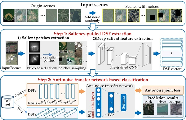
DSFATN consists of two main steps, as shown in Figure 1.
- Saliency-guided DSF extraction: To achieve discriminative high-level feature representation for RS scenes, we introduce saliency-guided DSF extraction. Instead of using the whole RS scene for feature extraction, saliency-guided DSF extraction produces a novel DSF representation based on saliency-guided RS scene patches using “visual attention” mechanisms. First, we conduct an improved patch-based visual saliency (PBVS) method to detect salient region and sample multi-scales salient patches in an image. Next, the multi-scales salient patches are fed to a pre-trained CNN model to extract the DSF. The saliency-guided DSF extraction ensures the most informative and representative parts are definitely centrally focused in the salient patches. Compared with randomly or densely sampling methods, the saliency-guided sampling is also more targeted and effective. The different scales of the salient patches also help to improve the scale invariance of DSF in the anti-noise transfer network training process.
- Anti-noise transfer network based classification: To suppress the influences of various scales and noises of RS scenes, an anti-noise transfer network is trained as the classifier successively. It introduces an anti-noise layer to tackle with DSFs extracted from RS scene patches in low quality even with various noises. Except for the anti-noise layer, the anti-noise transfer network only has a fully-connected (FC) layer and a softmax layer, which is a simple CNN architecture and can be trained easily. Different from the traditional CNN model, we optimize a new objective function to train the anti-noise transfer network by imposing an anti-noise constraint, which enforces the training samples before and after adding noises to share the similar features. Meanwhile, for anti-noise transfer network learning, the input scenes contain origin scenes and scenes with various noises, such as: (1) salt and pepper noise; (2) partial occlusions; and (3) their mixed noise. The whole framework works perfectly on three different scale RS scene datasets and even outperforms the state-of-the-art methods.
2.2. Saliency-Guided DSF Extraction
The saliency-guided DSF extraction provides the effective and discriminative high-level features from the most relevant scene patches using “visual attention” mechanisms. This extraction is inspired by the human visual system which interprets complex scenes in real time to get most relevant features of the scenes and reduce the complexity of scene analysis [40]. It also can be divided into two steps (Figure 1): (1) salient patch extraction; and (2) DSF extraction. The first step provides the scene patches sampled from the salient regions of input RS scenes. Inspired by graph-based visual saliency (GBVS) [41,42] method, we introduce a patch-based visual saliency (PBVS) algorithm to support the salient patch extractor. The second step is mainly accomplished by a pre-trained CNN, i.e., VGG-19 [19], where the 4096-dimensional activations of the first FC layer are used as the final DSFs.
2.2.1. Salient Patch Extraction
We improved the PBVS method for salient patch extraction. Different from traditional GBVS algorithm which can only detect the salient region from an image, our PBVS can provide multi-scales salient patches of the image. PBVS can be organized into the following procedures: (1) salient region detection; and (2) salient patch extraction. Figure 2 shows the flowchart of the PBVS based salient patch extraction. The details are described in the following section.
(1) Salient region detection. Given a set of scenes . For expository simplicity, suppose arbitrarily RS scene is a square image of size . At first step, PBVS extracts feature vectors at locations over to form the feature map of , is the value of locations in . The dissimilarity between and is defined as
Then, the activation map of needs to be formed. By connecting every node of the feature map , the fully connected directed graph is obtained. The directed edge from node to node of is assigned a weight, as shown in Equation (2). is a free parameter that is set to approximately 1/10 to 1/5 of the map width because it has been proven the results were not very sensitive to perturbations around these values. Then, the is treated as a Markov chain to compute the equilibrium distribution namely get the activation map . More details can be found in [41].
Then, activation map will be normalized to get the normalization map . Similar to the process of forming , another graph can be constructed based on activation map , but the weight assigned to the edges is defined as Equation (3). Again, a Markov chain on is obtained to help obtain the normalization map namely the final saliency map . If multiple activations were generated, these maps will be combined into one saliency map after normalization.
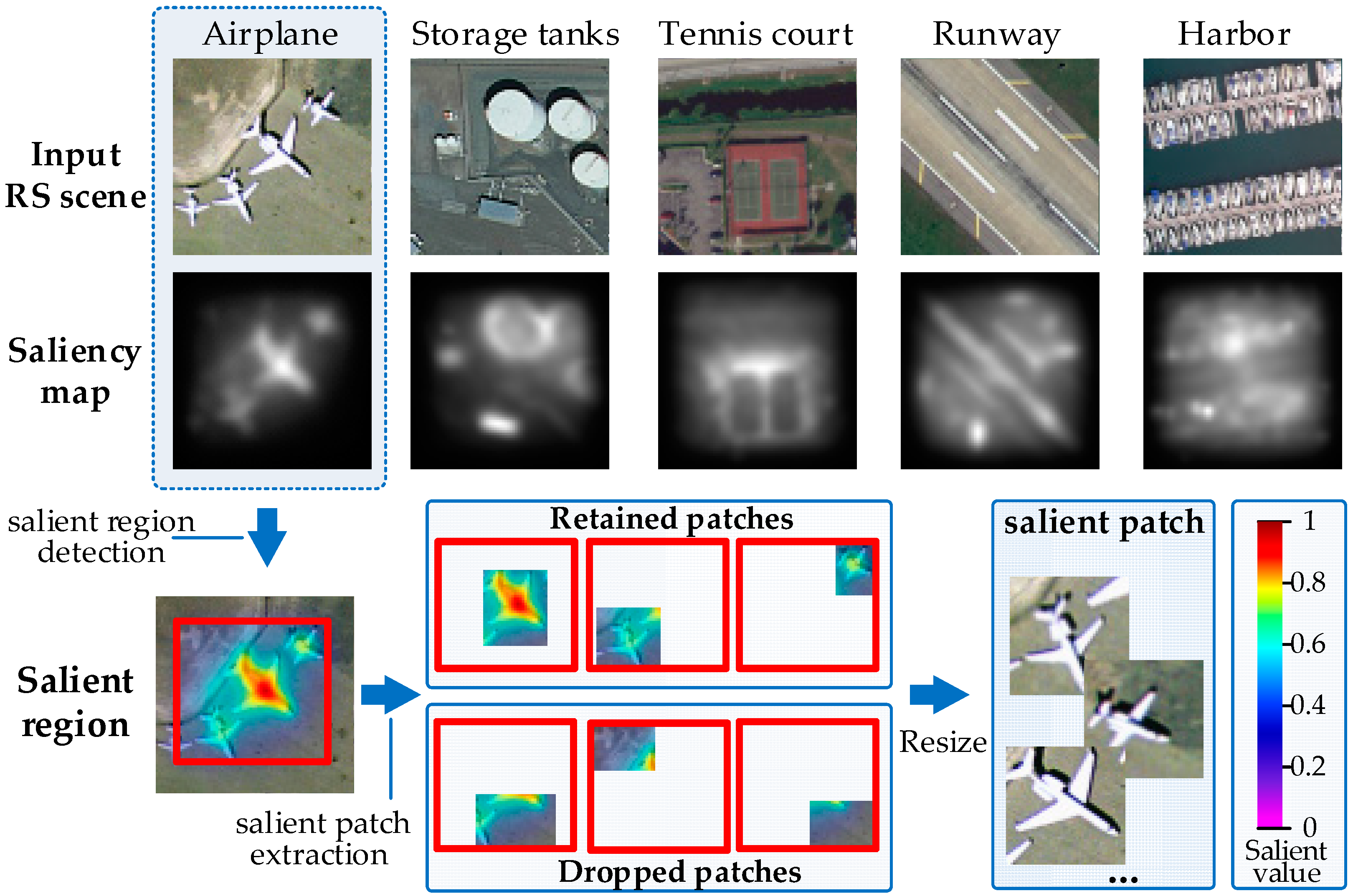
(2) Salient patch extraction. The Salient patch extraction provides multi-scales salient patches from the salient region. As shown in Figure 2, if an object is salient in the image, the corresponding location of its saliency map is high-lighted with bigger salient values. In an image, the salient values of its saliency map range from [0, 1], where 1 indicates the current location in the corresponding RS scene is the most salient, and 0 corresponds to the most non-salient. By finding the minimum bounding rectangle (MBR) [43] of the nonzero salient values in the saliency map , we primarily determine a salient region of RS scene s. Then, α patches will be sampled from by an iterative sampling procedure, where α is the threshold of patches’ number. The size of the patch can be scaled as the random rate from 30% to 80% of the salient region. The iterative sampling procedure prefers to sample the patches with bigger salient values in their central boxes, where the central box is defined as the central rectangle region of the sampled patch with its half width and height. In this work, we regard [0.8, 1] as the preferred salient value range to conduct the sampling process. Algorithm 1 shows the iterative sampling procedure for RS image scene s. At each iteration, a patch is randomly sampled in the salient region. If its salient values in the central box are all within the preferred salient value range , this patch should be considered as the salient patch and be kept, otherwise it should be dropped. The iteration will be continued until α patches with different scales are sampled. In our work, we set α = 9, and the influence of α will be discussed in Section 3.5.4.
| Algorithm 1. The iterative sampling procedure. | |
| Input: Salient region of RS image scene s | |
| Output: | |
| 1: | Initialization: |
| 2: | set salient patch set |
| 3: | set salient patches’ number |
| 4: | Iterations: |
| 5: | while () |
| 6: | randomly sampled a patch in |
| 7: | if (each salient value in central box) |
| 8: | put to P and note as in |
| 9: | |
| 10: | Return |
2.2.2. DSF Extraction
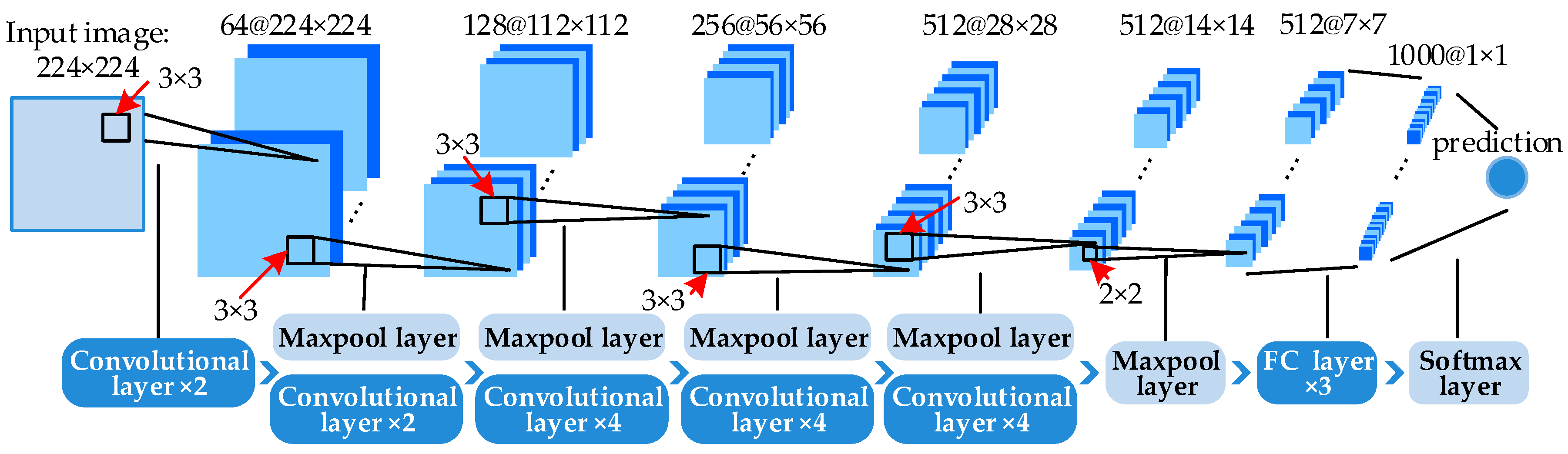
After selecting the training patches, we employed the VGG-19 architecture [19] (Figure 3) pre-trained with the ImageNet dataset to derive DSF representation. Additionally, we have compared different pre-trained CNN models in the Experimental Section and showed that VGG-19 performed the best. VGG-19 is one of the very deep CNN models proposed by Simonyan et al. [19]. Hu et al. [37] compared the performance of the activation vectors from different layers of the model, and found the activation vectors from the 1st FC layer are more capable to represent the image feature. Hence, the 4096-dimensional activation vector from the 1st FC layer of VGG-19 is adopted for deep salient feature representation in the case.
The pre-trained VGG-19 model includes 16 convolutional layers, five maxpool layers and three FC layers. When the multi-scales salient patches are fed to VGG-19 and preprocessed to the size of 224 × 224, the DSF can be extracted on the 1st FC layer. Supposing a set of scenes , the t-th DSF vector can be described as:
where returns scene added with the -th kind of noises (see Figure 1) and = 0 means none noise is added. PBVS function returns the -th salient patch of the corresponding scene. is the threshold of sampled salient patches, as described in Section 2.2.1. defines the deep feature extraction from the 1-st FC layer from VGG-19.
2.3. Anti-Noise Transfer Network Based Classification
Different from the traditional CNN models, an anti-noise transfer network is introduced to deal with the 4096-dimensional DSF vectors, as shown in Figure 4. The anti-noise transfer network is designed with simple architecture that can be trained easily with limited availability of the training data. It works well for DSFs of different RS scenes even with lower quality due to the anti-noise layer. The anti-noise layer imposes an anti-noise constraint to enforce the training samples before and after adding noises to share the similar output features. Thus, it can produce more robust and discriminative scene features to make the classification easier. Combining the anti-noise constraint to the softmax classification loss function, the anti-noise transfer network is learned by minimizing a joint loss, which is very different from the training of the traditional CNN models. The architecture and loss function of the anti-noise transfer network is described in detail below.
2.3.1. DSF Based Anti-Noise Transfer Network Architecture
As Figure 4 demonstrates, the anti-noise transfer network consists of two FC layers named FC1 and FC2 and a softmax layer, where rectified linear units (ReLU) [44] function is adopted to activate the output of FC1. FC1 and FC2 generate 4096-dimensional and N-dimensional vectors, respectively. N is the category number of the dataset. FC2 transfers the output vector of FC1 into N-dimensional vector thus it can be processed by softmax to produce the final classification results. The 4096-dimensional input DSF vector will be fed to anti-noise layer FC1 and activated by ReLU as:
where is the ReLU function, is the bias. Since the output of FC1 is 4096-dimensional, the weights . Analogously, will be processed by FC2 and the last softmax layer as follows:
where is the softmax function, is the bias. is N-dimensional, N equals the category number of scene categories, thus the weights . is also the final output of the transfer network . Setting , where is the i-th element of , the final prediction vector of can be represented as , which indicates the probabilities of the corresponding DSF belongs to each category. In the test phase, i-th category is the prediction label of when is the maximum element of .
2.3.2. Joint Loss Function Learning
To suppress the influence of noises, we propose a joint loss function to improve the anti-noise capability of the transfer network, where an anti-noise constraint is imposed to enforce the training samples before and after adding noise to share similar features. More specifically, for each training RS scene and its corresponding scene with the l-th noise , their DSFs and are enforced to generate similar output features in the transfer network by the anti-noise layer FC1. To achieve this goal, the novel joint loss function is proposed to learn parameters. Given the training RS scene set ={S}, their DSF set can be obtained as , where is the DSF set of origin scenes (e.g., ) and is the DSF set of corresponding scenes with the l-th () noise (e.g., ). is the true label set of . The joint loss value can be computed by:
where the first term is the softmax classification loss function and the second term is the anti-noise constraint. The joint loss is feedback for backpropagation update. Stochastic Gradient Descent (SGD) approach is employed here to solve the optimization problem, which is a widely used method for neural work training. By minimizing the joint loss value L, both the softmax classification loss and the distance between features extracted from training samples before and after adding noises are minimized.
The softmax classification loss is defined by Equation (8), where is the true label of , the first term of Equation (8) is the cross-entropy loss of , the second term is the L2 regularization to avoid over-fitting for better performance [45], is the weights of the anti-noise transfer network, and is the regularization coefficient, balance the weight between the two terms to be added, which is determined by the product of the weights decay.
The anti-noise constraint is proposed to enforce the training DSFs before and after adding noises to share the similar output features extracted by FC1, which introduced as the anti-noise layer in the transfer network. We define the constraint term by measuring the distance between DSFs before and after adding noises as:
where and are extracted from one RS scene before and after adding the l-th noises. is the number of , namely half of the joint number of the training samples.
By incorporating Equations (10) and (11) into Equation (9), the joint loss value is defined as:
3. Experiments and Analysis
3.1. Dataset and Experimental Protocol
Three different scale datasets are utilized; their specific categories are shown in Figure 5.
- UC Merced Land Use Dataset [1] (UCM) is collected from the large aerial orthoimagery of USGS National Map Urban Area Imagery collection. There are 100 images for each of 21 classes. Each image measures 256 × 256 pixels, with a 1-ft spatial resolution.
- The Google image dataset designed by RS_IDEA Group in Wuhan University (SIRI-WHU) [10] is acquired from Google Earth (Google Inc., Mountain View, CA, USA) and mainly covers urban areas in China. It contains 12 scene categories. Each class consists of 200 images with a size of 200 × 200 pixels and a spatial resolution of 2 m.
- SAT-6 dataset [46] is extracted from the National Agriculture Imagery Program and consists of a total of 405,000 image patches of size 28 × 28 and covering six classes. We choose 200 images from each class for our experiments.
All experiments are implemented with a 4.0 GHz Intel Core i7-6700K CPU, and two 8 GB GeFore GTX 1080 GPUs. We carried out experiments with five-fold cross-validation protocol on each RS scene dataset. The training set contained 80% of the RS scenes for each class, and the remaining scenes were used for testing. The numbers of training and test images of each RS scene dataset are listed in Table 1. Moreover, in this paper, three kinds of noise-adding strategies are applied: (1) salt and pepper noise with fixed noise density 0.1; (2) partial occlusion at random position that covers 20–30% of the image; and (3) their mixed noise. In the mixed noise strategy, origin scenes, scenes with salt and pepper noise and scenes with partial occlusion account 1/3 of the total scenes, respectively. Although much fewer images are utilized in this work than benchmark datasets such as ImageNet, DSFATN performs in different scales and noise conditions with great efficiency and robustness.
We mainly analyze the performance of DSFATN by the following aspects: (a) the effectiveness and applicability of DSFATN on the three different datasets; (b) the representation ability of DSF; (c) the robustness of the model by the anti-noise layer learning; and (d) the influence factors including patches’ number and pre-training models. Comparisons with the state-of-the-arts also demonstrate the superiority of our method.
3.2. Performance on Different Datasets
RS scenes from the three datasets employed in our experiments have a tremendous difference in image resolution and size. The UCM and SIRI-WHU datasets can provide different high-resolution RS scene images with proper image size, while the RS scenes from SAT-6 are really blurry with a quite small size. The diversity of the datasets can test DSFATN to the utmost.
(1) UCM dataset. We compared DSFATN with the state-of-the-arts such as the second extended spatial pyramid co-occurrence kernel (SPCK++) [13], pyramid-of-spatial-relations (PSR) [47], saliency-guided unsupervised feature learning (SG+UFL) [33] on the UCM dataset as shown in Table 2. Although most CNN methods can obtain results higher than 90%, especially the fine-tuning on GoogLeNet [34] get the second highest accuracy in the table, it is still 1.15% lower than the result of DSFATN. The CNN (including six convolutional layers and two FC layers) derived from [48] performs badly with the limited amount of data, while DSFATN deals with it well and obtains the highest accuracy, topping the accuracy of random forest (RF) [49] by almost 55%.
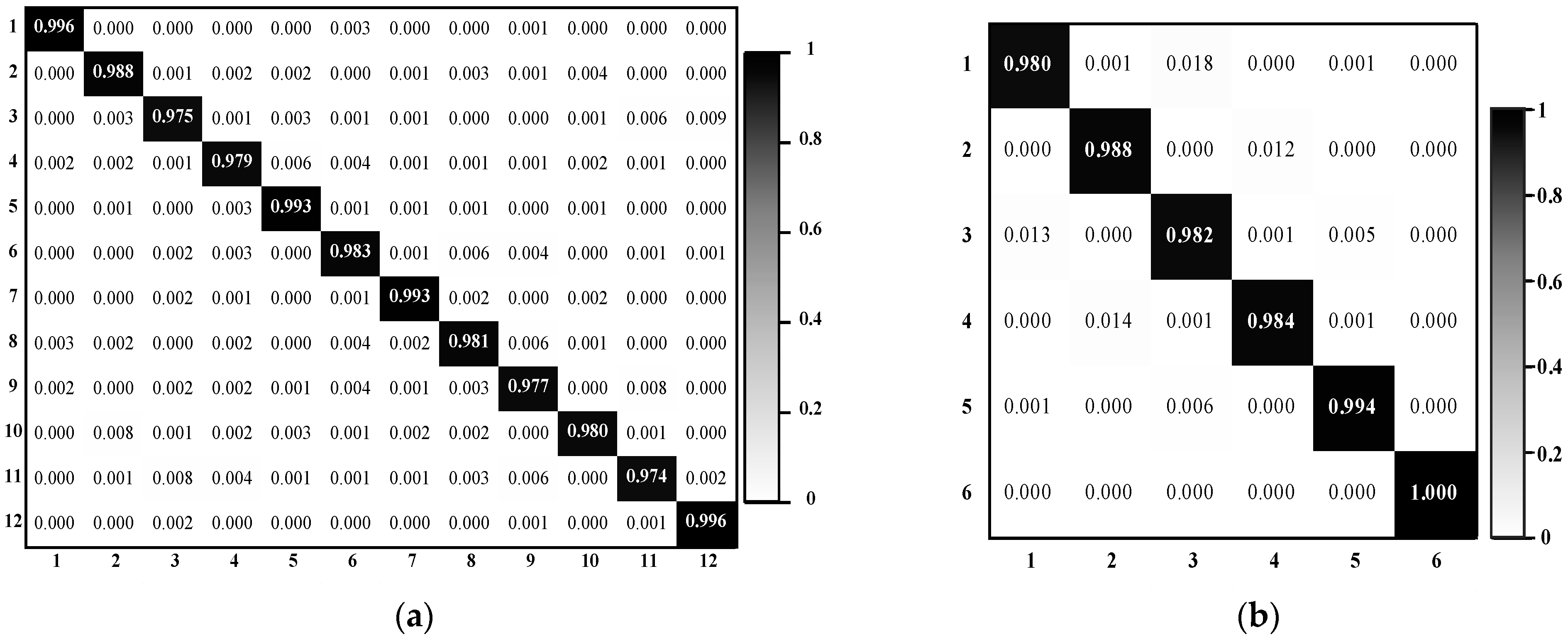
Figure 6 displays the confusion matrix of DSFATN on the UCM dataset. Most scenes can be classified into the right category, especially, the 6th class chaparral whose accuracy equals 1. While the 20th class storage tanks, as the lowest accuracy owner, are mistaken for several other classes, particularly the 5th category buildings and 14th category mobile home park, which is reasonable since some storage tanks are located on the roofs of buildings. The accuracy of storage tanks is higher than 96%, and the whole classification accuracy of DSFATN on the UCM dataset is quite satisfactory.
(2) SIRI-WHU dataset. Table 3 shows the results of DSFATN and several compared methods such Spatial Pyramid Matching (SPM) [12] on the SIRI-WHU dataset. Similar to the results on the UCM dataset, DSFATN obtains a high classification result of over 98%. RF and CNN(6conv+2fc) obtain the higher results than the UCM dataset because the SIRI-WHU dataset has fewer categories and more images in each category. It is obvious that DSFATN outperforms the other methods. Moreover, Figure 7a is the confusion matrix of DSFATN on the SIRI-WHU dataset. The accuracy of each category is higher than 97%. The worst misclassification probability is resulted by the 3rd class harbor: 0.9% of the harbor scenes are mistaken for 12th class water. The reason is that these two classes both consist of ship and water. For the same reason, the majority of the confusion occurs among categories that have the same component parts. For example, both the 2nd class commercial and 10th class residential consist of buildings and roads, while both the 9th class pond and the 11th class river are mainly made up of water. All categories achieve accuracies of over 97%.
(3) SAT-6 dataset. Note that the image scenes in the SAT-6 dataset are already salient patches with the dimension of from RS imageries. Even though the image resolution and scale in the SAT-6 dataset are identically low, DSFATN obtains the average accuracy of 98.80%, as shown in Table 4. The experiments show the impressive representation ability of DSFATN for small scale image scenes. Figure 7b is the confusion matrix of DSFATN on the SAT-6 dataset. Compared with results of the UCM and SIRI-WHU datasets, the misclassification probabilities of the SAT-6 dataset are much higher due to the high similarity between the scenes in smaller scale. The majority of the confusion occurs between the 1st class barren-land and the 3rd class grassland, and the 2nd class buildings and the 4th class roads, because these two pairs of categories have similar color and texture distribution, e.g., the former pair of categories both consist of green grass and brown earth.
3.3. Representative Ability Comparison of Different Features
In this section, to demonstrate the discriminative ability of DSF, we compared the DSF with several different features including histogram of oriented gradients (HOG) [50], scale invariant feature transform (SIFT) [51], and local binary patterns (LBP) [52], as shown in Table 5. For CNN(6conv+2fc), we extract its activations from the 1st FC layer as the representation features. After obtaining these features, we simply implement scene classification by training a linear support vector machine (SVM) classifier with each kind of features.
As Table 5 shows, no matter the accuracy or kappa coefficient, DSF obtained much higher results than other features on the three datasets. The high kappa values indicate the almost perfect coherence of DSF. On the UCM and SIRI-WHU datasets, the classification results of raw images are worse than the classification results of low-level features (e.g., HOG and LBP), and as expected both are worse than the classification results of high-level features extracted from CNNs including the CNN(6conv+2fc) feature and DSF. The raw images of SAT-6 perform much better than those low-level features owing to the characteristics of the SAT-6 dataset. The distinctive colors of the raw image in the SAT-6 dataset help a lot in the raw image classification but does not help in the low-level features extraction. Instead, the small image size and blurry image quality of SAT-6 image scenes make the low-level features extracted from raw images more unrepresentative. However, the features extracted from CNNs are discriminated, both the CNN(6conv+2fc) feature and DSF obtain accuracies over 90%. Especially the CNN(6conv+2fc) feature, although it does not perform well on the more complex UCM and SIRI-WHU datasets, it works quite well on the SAT-6 dataset due to the fewer categories and small RS scene image size of the SAT-6 dataset. The DSF performs more efficient and robust than the others in all three datasets.
Moreover, we embed the high-dimensional features to 2-D space by t-SNE [53], thus to visualize and compare the features extracted from these datasets. As shown in Figure 8, subfigures from top to bottom are the 2-D feature visualization images of HOG, LBP, SIFT, CNN(6conv+2fc) feature and DSF in order, and from left to right are the 2-D feature visualization images of the UCM, SIRI-WHU and SAT-6 datasets respectively. Each color in the images represents a category in the corresponding dataset. Obviously, the 2-D features of HOG, SIFT, and LBP are distributed disordered and only form very few clusters. In contrast, the 2-D features of DSF form clusters separated much clearly. Moreover, the 2-D features of CNN(6conv+2fc) also form more clusters than HOG, SIFT and LBP since the high-level features that contain more abstract semantic information than the low-level features. Notice that CNN(6conv+2fc) feature performs very well in the SAT-6 dataset, obtaining a high result of 94.58%, which very close to the result 96.25% obtained by DSF; this is also reflected in the 2-D feature visualization images, both kinds of features can form the main six clusters. Barren-land class, grassland class and trees class are very close to each other and have some overlap, since in the small scale and resolution SAT-6 dataset, these three categories all consist of soils and vegetation with different vegetation cover rate. The grassland has a middle vegetation plant cover rate; therefore, its features locate between features of barrenland and trees. The buildings class and the roads class have similar situations because the roof of the buildings and the roads are both mainly made up of cement concrete. Particularly, the water class is not similar to the five other categories, and the overlap between the grassland class and the water class in the CNN (6conv+2fc) situation turns out to be unreasonable. While the DSFATN discriminates the difference since the pink area that represents the water features locates far away from the five other categories. Moreover, compared with DSFATN, the CNN(6conv+2fc) feature generates more points that do not locate in the clusters they belong to. In general, DSF learns to be more discriminative.
3.4. Evaluation of Image Distortion
In this section, we validate the robustness of DSFATN for two kinds image distortion conditions: (1) images with noises; and (2) images in different scales. In Section 3.2, we have already proven DSFATN worked well on the SAT-6 dataset which contains RS scenes in small scale and low resolution, thus, in this section, we perform the anti-noise tests on the UCM and SIRI-WHU datasets.
3.4.1. Evaluation of Noises
To validate the anti-noise ability of DSFATN, we compared DSFATN with several different methods under three kinds of noise. Particularly, to prove the indispensability and effectiveness of multi-scales salient patches and anti-noise layer, two variant models derived from DSFATN are introduced. Table 6 lists their difference with the proposed DSFATN. TN-1 refers to DSFATN without multi-scales salient patches sampling and anti-noise layer training. TN-2 refers to DSFATN without multi-scales salient patches sampling but with anti-noise layer training. The absence of anti-noise layer training is simply achieved by learning the joint loss without the anti-noise constraint.
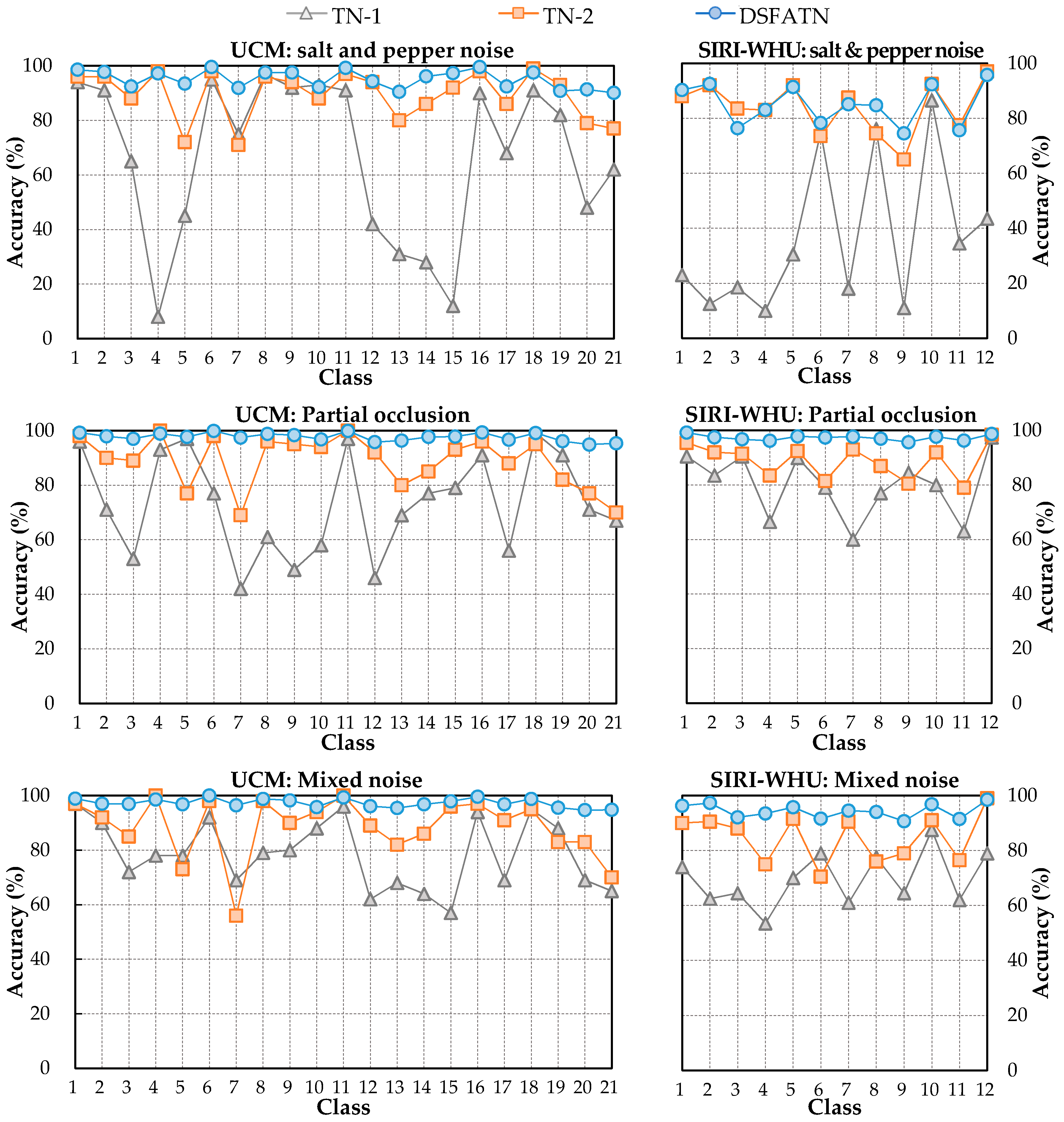
Table 7 compares the models on the UCM dataset and the SIRI-WHU dataset. Obviously, RF and CNN(6conv+2fc) have a very weak anti-noise property for obtaining accuracies less than 50% with all three kinds of noises, while the classification results of DSFATN are all above 95%. In particular, the result difference between TN-2 and DSFATN almost reaches 10%, which indicates the great importance of saliency patches sampling. Analogously, TN-1 has much worse results compared with TN-2, where the result difference even reaches 47.66% on the SIRI-WHU dataset with salt and pepper noise. The averaged result difference between TN-1 and TN-2 on the UCM and SIRI-WHU datasets with the three kinds of noises reaches 19.92%, which shows the effectiveness of anti-noise layer. As expected, on both the UCM and SIRI-WHU datasets, the results with the three kinds of noises rank in the order: TN-1 < TN-2 < DSFATN. This reflects the important role played by salient patches and the anti-noise layer.
Figure 9 shows the per-class accuracies of TN-1, TN-2, and DSFATN on the UCM and SIRI-WHU datasets with the three kinds of noises. Similar to the trend of the whole results, in most cases, the accuracies are in the following order: DSFATN > TN-2 > TN-1. It is interesting to find that TN-1 and TN-2 perform well in several classes with accuracies over 90%, which even equal or exceed the results of DSFATN, such as the 1st class agricultural, the 11th class harbor, the 16th class overpass, the 18th class runway of the UCM dataset and the 12th class water of the SIRI-WHU dataset. These scenes including duplicate texture information (e.g., ships, water, roads, and roads) make saliency detection confusing. Moreover, irrelevant objects (e.g., a ship in the water class scene) occasionally appearing misled the saliency detection results. Nevertheless, TN-1 and TN-2 behave poor in the other categories, and the corresponding accuracies dropped in different degrees. In general, on both the UCM and SIRI-WHU datasets, TN-2 obtains mediocre performance, better than TN-1 and worse than DSFATN, while TN-1 obtains quite uneven results—most of its results are below 80%. In sharp contrast to this is the stable performance of the DSFATN, which ensures most results are higher than 90%.
To further confirm the ability of the anti-noise layer FC1 in the anti-noise transfer network, we compare the FC1 layer’s output feature with different features under the three kinds of noises (see Table 8), similar to in Section 3.3. Compared with the accuracies in Table 5, the results of corresponding features in Table 8 have declined in different degrees due to the influence of the noises. CNN(6con+2fc) feature and DSF show some superiority compared with the low-level features in this anti-noise experiments, obtaining accuracies even higher than the results obtained by the low-level features extracted from origin RS scene images without any noise (see Table 5). However, it is not robust enough to represent the images with noises. The last row of Table 8 shows the accuracies obtained by features extracted from the FC1 layer; most of them are higher than 0.90, and all the results are significantly enhanced compared to the results classified by DSF. The great difference between DSF and indicates introducing the FC1 layer to the anti-noise transfer network is indeed very important.
3.4.2 Evaluation of Multiple Scales
To evaluate the impact of image scale, we resized the RS scene images from the UCM and SIRI-WHU datasets to five different scales, i.e., a quarter of original image size (height and width dimensions), half of original image size, three quarters of original image size, original image size and one and a quarter size.
We compared DSFATN with CNN(6conv+2fc) and the TN-2 model. As the results in Table 9 and Table 10 show, DSFTAN performs the best on the UCM and SIRI-WHU datasets at all five scales. Almost all the accuracies are over 98%, and the results of DSFATN are quite stable for obtaining the lowest STD value. The results of CNN(6conv+2fc) are very unstable with the image scale variances. Particularly, TN-2, which does not conduct multi-scales patches sampling, compared with DSTATN, also obtained high accuracies around 90% on the two datasets. However, the STD values of TN-2 are much higher. Moreover, the UCM, SIRI-WHU and SAT-6 datasets also have different scales and resolutions, especially the SAT-6 dataset. Our method demonstrated robustness across the three datasets.
3.5. The Analysis of Influence Factors
In this section, we analyze several influence factors in DSFATN: (a) the threshold of salient patches’ number α; (b) the regularization coefficient λ; (c) the pre-trained CNN models; and (d) the noise level. For simplicity and equity, all comparison experiments were conducted on the UCM dataset.
3.5.1. Influence of Salient Patches’ Number α
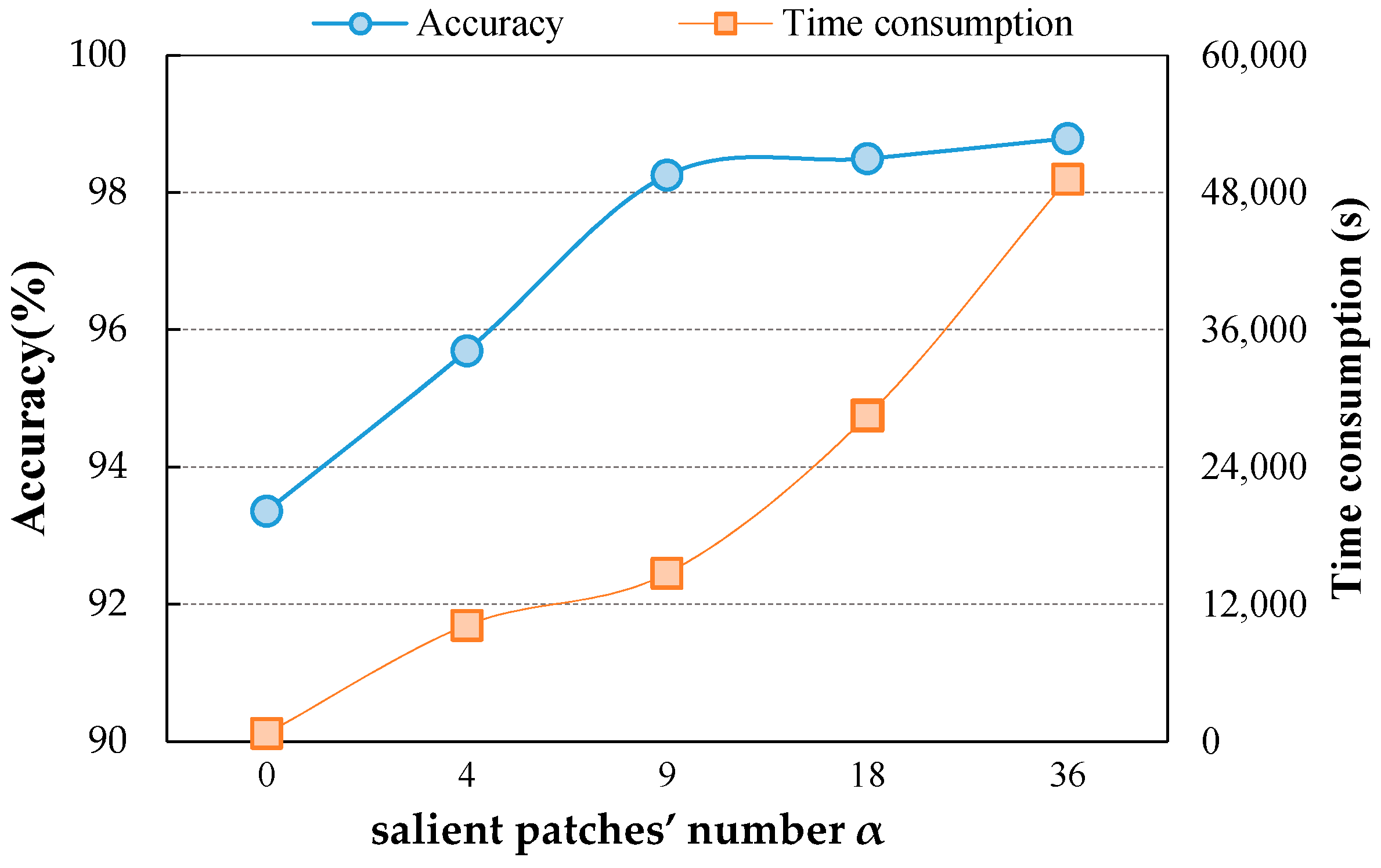
Figure 10 shows the influence of salient patches’ number α. Time consumption refers to the time for obtaining all the DSF of the RS image scenes utilized in the corresponding experiments. means salient regions are not detected thus the DSF are directly extracted from the origin image scenes. As α increases from 0 to 9, the time consumption increases slowly while the accuracy rises sharply. When , the accuracy keeps a flat level of growth while the time consumption steepens. Only when , a high classification accuracy can be gained without much time consumption. Hence, is selected in our method.
3.5.2. Influence of the Regularization Coefficient
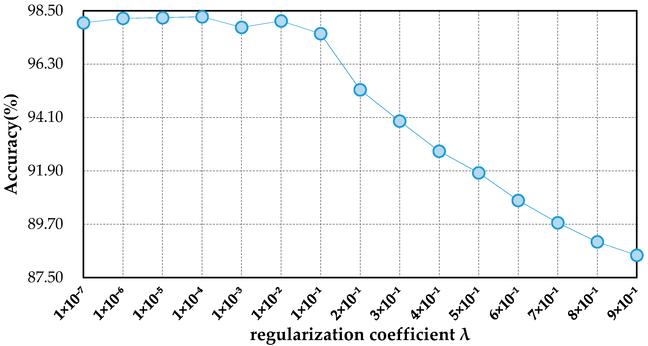
Figure 11 shows the classification results of DSFATN in different regularization coefficient . When is very small (i.e., ), DSFATN performs quite good, and the accuracy levels out at around 98%. When is assigned bigger values (i.e., ), the accuracy declines fast. When , DSFATN achieves the highest result.
3.5.3. Influence of Pre-Trained CNNs
We changed the pre-trained CNN in DSFATN from VGG-19 to several other kinds of CNNs, while keeping the rest of the structure of DSFATN unchanged. Table 11 presents the classification results of different pre-trained CNNs. Note that, for the pre-trained CNN models which contain three FC layers (Rows 1–7), we extracted the features from the 1st FC layer as the feature presentation. For the other per-trained CNNs (Rows 8–15), we regarded the output of the layer that generate one-dimensional vectors (e.g., logits layer in InceptionV3) as the representation. All extracted representations have the same anti-noise transfer network architecture but are trained separately. As shown in Table 11, compared with VGG-19, most pre-trained CNNs can achieve comparable results over 96% (e.g., Rows 1–6 and 11–12). Although the inception models perform well too, they are not so competitive with other models for deep feature extraction, since they are not deep enough compared with Resnetv1_50 and Resnetv1_101. The fully connected layers, which appear in each traditional CNNs (e.g., Rows 1–7), play a great role for deep feature extraction. Nevertheless, the results of inceptions are still higher than 90%. One can see that our DSFATN with VGG-19 outperforms the others.
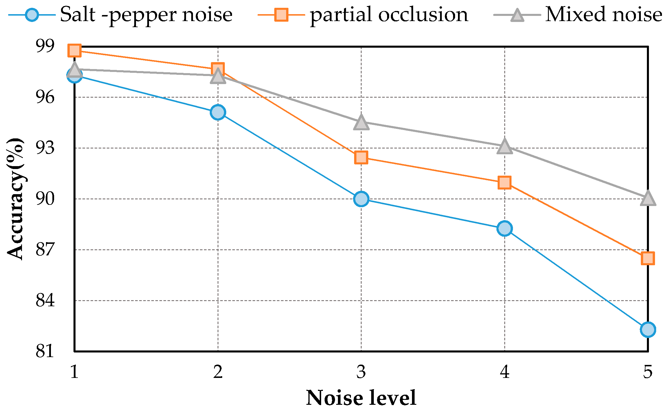
3.5.4. Influence of Noise Levels
We investigate the robustness sensitivity of DSFATN at five different levels of noises. Table 12 shows the parameters of the salt and pepper noise and partial occlusion at these five levels of noise conditions; the mixed noise is still the mixture of the former two kinds noise and original image scenes with the same proportion. Note that Level 2 noise condition has been adopted as the setting in the preceding experiment part (see Section 3). Figure 12 demonstrates these five noise levels of an example tennis court scene. Obviously, when the noise level becomes higher, the scenes with salt and pepper noise are blurrier with more noise pixels, and the scenes with partial occlusion are covered with larger black region. At Levels 3–5, the tennis court cannot be seen in the image scene.
The average accuracies of DSFATN at these five noise levels are shown in Figure 13. As expected, the higher the noise level is, the lower the classification accuracy is. In salt and pepper noise condition, the salt and pepper noise with higher noise level brings more noise pixels to the scene, which makes the performance of saliency detection degenerate. In partial occlusion condition, the higher partial occlusion level leads to the semantic information loss. When the noise level is higher than 2, the results of salt and pepper noise and partial collusion conditions declines more sharply than the result of mixed noise condition. The origin scenes in the mixed noise condition, which supplement the information loss caused by the salt and pepper noise and partial occlusion to some extent. In general, although the accuracies have a declining trend, all results are higher than 80%, even for partial occlusion covering almost half scale of the scenes. The results are also higher than the accuracies obtained by some traditional methods in the origin scenes without any noises (see Table 2).
4. Conclusions
This paper proposes a deep salient feature based anti-noise transfer network (DSFATN) method for RS scene classification with different scales and various noises. In DSFATN, the saliency-guided DSF extraction extracts the discriminative high-level DSF from the most relevant, informative and representative patches of the RS scene sampled by the Patch-Based Visual Saliency (PBVS) method. The VGG-19 is selected as the pre-trained CNN to extract DSF among various candidate CNNs for its better performance. DSF achieves discriminative high-level feature representation learned from pre-trained VGG-19 for the RS scenes. Meanwhile, an anti-noise transfer network is introduced to learn and enhance the robust and anti-noise structure information of RS scene by directly propagating the label information to fully-connected layers. By minimizing the joint loss concerning anti-noise constraint and softmax classification loss simultaneously, the anti-noise transfer network can be trained easily with limited amount of data and without accuracy loss. DSFATN performs excellent with RS scenes in different quality, even with noise.
The results on three different scale datasets with limited data are encouraging: the classification results are all above 98%, which outperforms the results of state-of-the-art methods. DSFATN also obtains satisfactory results under various noises. For example, the results on the widespread UCM with noises are higher than 95%, which is even better than the best results of some state-of-the-art methods on UCM without noise. The remarkable results indicate the effectiveness and wide applicability of DSFATN and prove the robustness of DSFATN.
However, the strong anti-noise property of DSFATN is dependent on different datasets; for example, under salt and pepper noise, the accuracy of DSFATN reaches 95.12% on the UCM dataset while it dropped to 84.98% on the SIRI-WHU dataset. In the future, we will conduct an end-to-end multi-scale and multi-channel network to jointly extract more adaptive representation for RS scene with limited availability of training data for complex scene understanding.
Acknowledgments
This study was financially supported by the National Natural Science Foundation of China (No. 41671400, No. 41701446 and No. 61602429); National key R & D program of China (No. 2017YFC0602204); Hubei Natural Science Foundation of China (2015CFA012).
Author Contributions
Yuanyuan Liu and Zhong Xie conceived and designed the experiments. Xi Gong and Zhuo Zheng performed the experiments. Yuanyuan Liu and Xi Gong contributed to the analysis. The manuscript was written by Xi Gong with contributions from Yuanyuan Liu, Xuguo Shi.
Conflicts of Interest
The authors declare no conflict of interest.
References
- Yang, Y.; Newsam, S. Bag-of-visual-words and spatial extensions for land-use classification. In Proceedings of the 18th SIGSPATIAL International Conference on Advances in Geographic Information Systems, San Jose, CA, USA, 3–5 November 2010; pp. 270–279. [Google Scholar]
- Cheriyadat, A.M. Unsupervised feature learning for aerial scene classification. IEEE Trans. Geosci. Remote Sens. 2014, 52, 439–451. [Google Scholar] [CrossRef]
- Yang, W.; Yin, X.; Xia, G.S. Learning high-level features for satellite image classification with limited labeled samples. IEEE Trans. Geosci. Remote Sens. 2015, 53, 4472–4482. [Google Scholar] [CrossRef]
- Shao, W.; Yang, W.; Xia, G.S. Extreme value theory-based calibration for the fusion of multiple features in high-resolution satellite scene classification. Int. J. Remote Sens. 2013, 34, 8588–8602. [Google Scholar] [CrossRef]
- Wang, Q.; Meng, Z.; Li, X. Locality Adaptive Discriminant Analysis for Spectral–Spatial Classification of Hyperspectral Images. IEEE Geosci. Remote Sens. Lett. 2017, 14, 2077–2081. [Google Scholar] [CrossRef]
- Bosch, A.; Muñoz, X.; Martí, R. Which is the best way to organize/classify images by content? Image Vis. Comput. 2007, 25, 778–791. [Google Scholar] [CrossRef]
- Zhong, Y.; Zhu, Q.; Zhang, L. Scene classification based on the multifeature fusion probabilistic topic model for high spatial resolution remote sensing imagery. IEEE Trans. Geosci. Remote Sens. 2015, 53, 6207–6222. [Google Scholar] [CrossRef]
- Zhou, L.; Zhou, Z.; Hu, D. Scene classification using a multi-resolution bag-of-features model. Pattern Recognit. 2013, 46, 424–433. [Google Scholar] [CrossRef]
- Zhao, B.; Zhong, Y.; Zhang, L.; Huang, B. The fisher kernel coding framework for high spatial resolution scene classification. Remote Sens. 2016, 8, 157. [Google Scholar] [CrossRef]
- Zhao, B.; Zhong, Y.; Xia, G.-S.; Zhang, L. Dirichlet-derived multiple topic scene classification model fusing heterogeneous features for high spatial resolution remote sensing imagery. IEEE Trans. Geosci. Remote Sens. 2016, 54, 2108–2123. [Google Scholar] [CrossRef]
- Zhong, Y.; Fei, F.; Zhang, L. Large patch convolutional neural networks for the scene classification of high spatial resolution imagery. J. Appl. Remote Sens. 2016, 10, 025006. [Google Scholar] [CrossRef]
- Lazebnik, S.; Schmid, C.; Ponce, J. Beyond bags of features: Spatial pyramid matching for recognizing natural scene categories. In Proceedings of the IEEE Conference on Computer Vision and Pattern Recognition, New York, NY, USA, 17–22 June 2006; Volume 2, pp. 2169–2178. [Google Scholar]
- Yang, Y.; Newsam, S. Spatial pyramid co-occurrence for image classification. In Proceedings of the IEEE International Conference on Computer Vision, Barcelona, Spain, 6–13 November 2011; pp. 1465–1472. [Google Scholar]
- Blei, D.M.; Ng, A.Y.; Jordan, M.I. Latent dirichlet allocation. J. Mach. Learn. Res. 2003, 3, 993–1022. [Google Scholar]
- Lienou, M.; Maitre, H.; Datcu, M. Semantic annotation of satellite images using latent dirichlet allocation. IEEE Geosci. Remote Sens. Lett. 2010, 7, 28–32. [Google Scholar] [CrossRef]
- Vaduva, C.; Gavat, I.; Datcu, M. Latent dirichlet allocation for spatial analysis of satellite images. IEEE Trans. Geosci. Remote Sens. 2013, 51, 2770–2786. [Google Scholar] [CrossRef]
- Bosch, A.; Zisserman, A.; Muñoz, X. Scene classification using a hybrid generative/discriminative approach. IEEE Trans. Pattern Anal. Mach. Intell. 2008, 30, 712–727. [Google Scholar] [CrossRef] [PubMed]
- Cheng, G.; Guo, L.; Zhao, T.; Han, J.; Li, H.; Fang, J. Automatic landslide detection from remote-sensing imagery using a scene classification method based on BoVW and pLSA. Int. J. Remote Sens. 2013, 34, 45–59. [Google Scholar] [CrossRef]
- Simonyan, K.; Zisserman, A. Very deep convolutional networks for large-scale image recognition. In Proceedings of the International Conference on Learning Representations, San Diego, CA, USA, 7–9 May 2015. [Google Scholar]
- Zou, Z.; Shi, Z. Ship detection in spaceborne optical image with SVD networks. IEEE Trans. Geosci. Remote Sens. 2016, 54, 5832–5845. [Google Scholar] [CrossRef]
- Gao, J.; Wang, Q.; Yuan, Y. Embedding structured contour and location prior in siamesed fully convolutional networks for road detection. In Proceedings of the IEEE International Conference on Robotics and Automation, Singapore, 29 May–3 June 2017; pp. 219–224. [Google Scholar]
- Li, C.; Wand, M. Combining markov random fields and convolutional neural networks for image synthesis. arXiv, 2016; arXiv:1601.04589. [Google Scholar]
- Zhang, L.; Zhang, L.; Du, B. Deep Learning for Remote Sensing Data: A Technical Tutorial on the State of the Art. IEEE Geosci. Remote Sens. Mag. 2016, 4, 22–40. [Google Scholar] [CrossRef]
- Zhu, X.X.; Tuia, D.; Mou, L.; Xia, G.S.; Zhang, L.; Xu, F. Deep Learning in Remote Sensing: A Comprehensive Review and List of Resources. IEEE Geosci. Remote Sens. Mag. 2017, 5, 8–36. [Google Scholar] [CrossRef]
- Lu, X.; Zheng, X.; Yuan, Y. Remote sensing scene classification by unsupervised representation learning. IEEE Trans. Geosci. Remote Sens. 2017, 55, 5148–5157. [Google Scholar] [CrossRef]
- Chen, Y.; Zhao, X.; Jia, X. Spectral–spatial classification of hyperspectral data based on deep belief network. IEEE J. Sel. Top. Appl. Earth Obs. Remote Sens. 2015, 8, 2381–2392. [Google Scholar] [CrossRef]
- Deng, J.; Dong, W.; Socher, R.; Li, L.J.; Li, K.; Fei-Fei, L. Imagenet: A large-scale hierarchical image database. In Proceedings of the IEEE Conference on Computer Vision and Pattern Recognition, Miami, FL, USA, 20–25 June 2009; pp. 248–255. [Google Scholar]
- Li, H.; Fu, K.; Yan, M.; Sun, X.; Sun, H.; Diao, W. Vehicle detection in remote sensing images using denoising-based convolutional neural networks. Remote Sens. Lett. 2017, 8, 262–270. [Google Scholar] [CrossRef]
- Yang, Y.; Zhuang, Y.; Bi, F.; Shi, H.; Xie, Y. M-FCN: Effective fully convolutional network-based airplane detection framework. IEEE Geosci. Remote Sens. Lett. 2017, 14, 1293–1297. [Google Scholar] [CrossRef]
- Chen, X.; Xiang, S.; Liu, C.L.; Pan, C.H. Vehicle detection in satellite images by hybrid deep convolutional neural networks. IEEE Geosci. Remote Sens. Lett. 2017, 11, 1797–1801. [Google Scholar] [CrossRef]
- Simard, P.Y.; Steinkraus, D.; Platt, J.C. Best practices for convolutional neural networks applied to visual document analysis. In Proceedings of the Seventh International Conference on Document Analysis and Recognition, Edinburgh, UK, 3–6 August 2003; pp. 958–962. [Google Scholar]
- Dieleman, S.; Willett, K.W.; Dambre, J. Rotation-invariant convolutional neural networks for galaxy morphology prediction. Mon. Not. R. Astron. Soc. 2015, 450, 1441–1459. [Google Scholar] [CrossRef]
- Zhang, F.; Du, B.; Zhang, L. Saliency-guided unsupervised feature learning for scene classification. IEEE Trans. Geosci. Remote Sens. 2015, 53, 2175–2184. [Google Scholar] [CrossRef]
- Castelluccio, M.; Poggi, G.; Sansone, C.; Verdoliva, L. Land use classification in remote sensing images by convolutional neural networks. arXiv, 2015; arXiv:1508.00092. [Google Scholar]
- Szegedy, C.; Liu, W.; Jia, Y.; Sermanet, P.; Reed, S.; Anguelov, D. Going deeper with convolutions. In Proceedings of the IEEE Conference on Computer Vision and Pattern Recognition, Boston, MA, USA, 11–12 June 2015; pp. 1–9. [Google Scholar]
- Penatti, O.A.; Nogueira, K.; dos Santos, J.A. Do deep features generalize from everyday objects to remote sensing and aerial scenes domains? In Proceedings of the IEEE Conference on Computer Vision and Pattern Recognition Workshops, Boston, MA, USA, 12 June 2015; pp. 44–51. [Google Scholar]
- Hu, F.; Xia, G.S.; Hu, J.; Zhang, L. Transferring deep convolutional neural networks for the scene classification of high-resolution remote sensing imagery. Remote Sens. 2015, 7, 14680–14707. [Google Scholar] [CrossRef]
- Gong, Y.; Wang, L.; Guo, R.; Lazebnik, S. Multi-scale orderless pooling of deep convolutional activation features. In The European Conference on Computer Vision (ECCV); Springer: Cham, Swizerland, 2014; pp. 392–407. [Google Scholar]
- Lee, H.; Grosse, R.; Ranganath, R.; Ng, A.Y. Convolutional deep belief networks for scalable unsupervised learning of hierarchical representations. In Proceedings of the 26th annual international conference on machine learning, Montreal, QC, Canada, 14–18 June 2009; pp. 609–616. [Google Scholar]
- Itti, L.; Koch, C.; Niebur, E. A model of saliency-based visual attention for rapid scene analysis. IEEE Trans. Pattern Anal. Mach. Intell. 1998, 20, 1254–1259. [Google Scholar] [CrossRef]
- Harel, J.; Koch, C.; Perona, P. Graph-based visual saliency. In Proceedings of the Advances in Neural Information Processing Systems, Vancouver, BC, Canada, 3 December 2007; pp. 545–552. [Google Scholar]
- Harel, J. A Saliency Implementation in MATLAB. Available online: http://www.vision.caltech.edu/~harel/share/gbvs.php (accessed on 10 January 2018).
- Caldwell, D.R. Unlocking the mysteries of the bounding box. Coord. Online J. Map Geogr. Round Tab. Am. Libr. Assoc. 2005. Available online: http://www.stonybrook.edu/libmap/coordinates/seriesa/no2/a2.pdf (accessed on 10 January 2018).
- Glorot, X.; Bordes, A.; Bengio, Y. Deep sparse rectifier neural networks. In Proceedings of the Fourteenth International Conference on Artificial Intelligence and Statistics, Lauderdale, FL, USA, 11–13 April 2011; pp. 315–323. [Google Scholar]
- Peng, X.; Lu, C.; Yi, Z.; Tang, H. Connections between Nuclear Norm and Frobenius-Norm-Based Representations. IEEE Trans. Neural Netw. Learn. Syst. 2016. [Google Scholar] [CrossRef] [PubMed]
- Basu, S.; Ganguly, S.; Mukhopadhyay, S.; Dibiano, R.; Karki, M.; Nemani, R. Deepsat: A learning framework for satellite imagery. In Proceedings of the 23rd ACM SIGSPATIAL International Conference on Advances in Geographic Information Systems, Seattle, WA, USA, 3–6 November 2015; p. 37. [Google Scholar]
- Chen, S.; Tian, Y. Pyramid of spatial relatons for scene-level land use classification. IEEE Trans. Geosci. Remote Sens. 2015, 53, 1947–1957. [Google Scholar] [CrossRef]
- Krizhevsky, A.; Sutskever, I.; Hinton, G.E. ImageNet classification with deep convolutional neural networks. In Proceedings of the Twenty-Sixth International Conference on Neural Information Processing Systems, Lake Tahoe, NY, USA, 3–8 December 2012; pp. 1097–1105. [Google Scholar]
- Breiman, L. Random forests. Mach. Learn. 2001, 45, 5–32. [Google Scholar] [CrossRef]
- Dalal, N.; Triggs, B. Histograms of oriented gradients for human detection. In Proceedings of the IEEE Computer Society Conference on Computer Vision and Pattern Recognition, San Diego, CA, USA, 20–26 June 2005; pp. 886–893. [Google Scholar] [CrossRef]
- Lowe, D.G. Distinctive image features from scale-invariant keypoints. Int. J. Comput. Vis. 2004, 60, 91–110. [Google Scholar] [CrossRef]
- Ojala, T.; Pietikainen, M.; Maenpaa, T. Multiresolution gray-scale and rotation invariant texture classification with local binary patterns. IEEE Trans. Pattern Anal. Mach. Intell. 2002, 24, 971–987. [Google Scholar] [CrossRef]
- Van der Maaten, L.; Hinton, G. Visualizing data using t-SNE. J. Mach. Learn. Res. 2008, 9, 2579–2605. [Google Scholar]
- Jia, Y.; Shelhamer, E.; Donahue, J.; Karayev, S.; Long, J.; Girshick, R.; Guadarrama, S.; Darrell, T. Caffe: Convolutional architecture for fast feature embedding. In Proceedings of the ACM International Conference on Multimedia, Orlando, FL, USA, 3–7 November 2014. [Google Scholar]
- Chatfield, K.; Simonyan, K.; Vedaldi, A.; Zisserman, A. Return of the devil in the details: Delving deep into convolutional nets. In Proceedings of the British Machine Vision Conference, Nottingham, UK, 1–5 September 2014. [Google Scholar]
- Ioffe, S.; Szegedy, C. Batch normalization: Accelerating deep network training by reducing internal covariate shift. In Proceedings of the International Conference on Machine Learning, Lille, France, 6–11 July 2015; pp. 448–456. [Google Scholar]
- Szegedy, C.; Vanhoucke, V.; Ioffe, S.; Shlens, J.; Wojna, Z. Rethinking the inception architecture for computer vision. In Proceedings of the IEEE Conference on Computer Vision and Pattern Recognition, Las Vegas, NV, USA, 26 June–1 July 2016; pp. 2818–2826. [Google Scholar]
- He, K.; Zhang, X.; Ren, S.; Sun, J. Deep residual learning for image recognition. In Proceedings of the IEEE conference on computer vision and pattern recognition, Las Vegas, NV, USA, 26 June–1 July 2016; pp. 770–778. [Google Scholar]
Figure 1.
The framework of deep salient feature based anti-noise transfer network (DSFATN) contains two main steps: saliency-guided deep salient feature (DSF) extraction and anti-noise transfer network based classification. The saliency-guided DSF extraction conducts a patch-based visual saliency (PBVS) to guide pre-trained convolutional neural networks (CNNs) for producing the discriminative high-level DSF for remote sensing (RS) scene with different scale and various noises. Then, the anti-noise transfer network is trained to learn and enhance the robust and anti-noise structure information of RS scene by minimizing a joint loss. For anti-noise learning, the input scenes include origin scenes and scenes with various noises (e.g., salt and pepper, occlusions and mixtures).
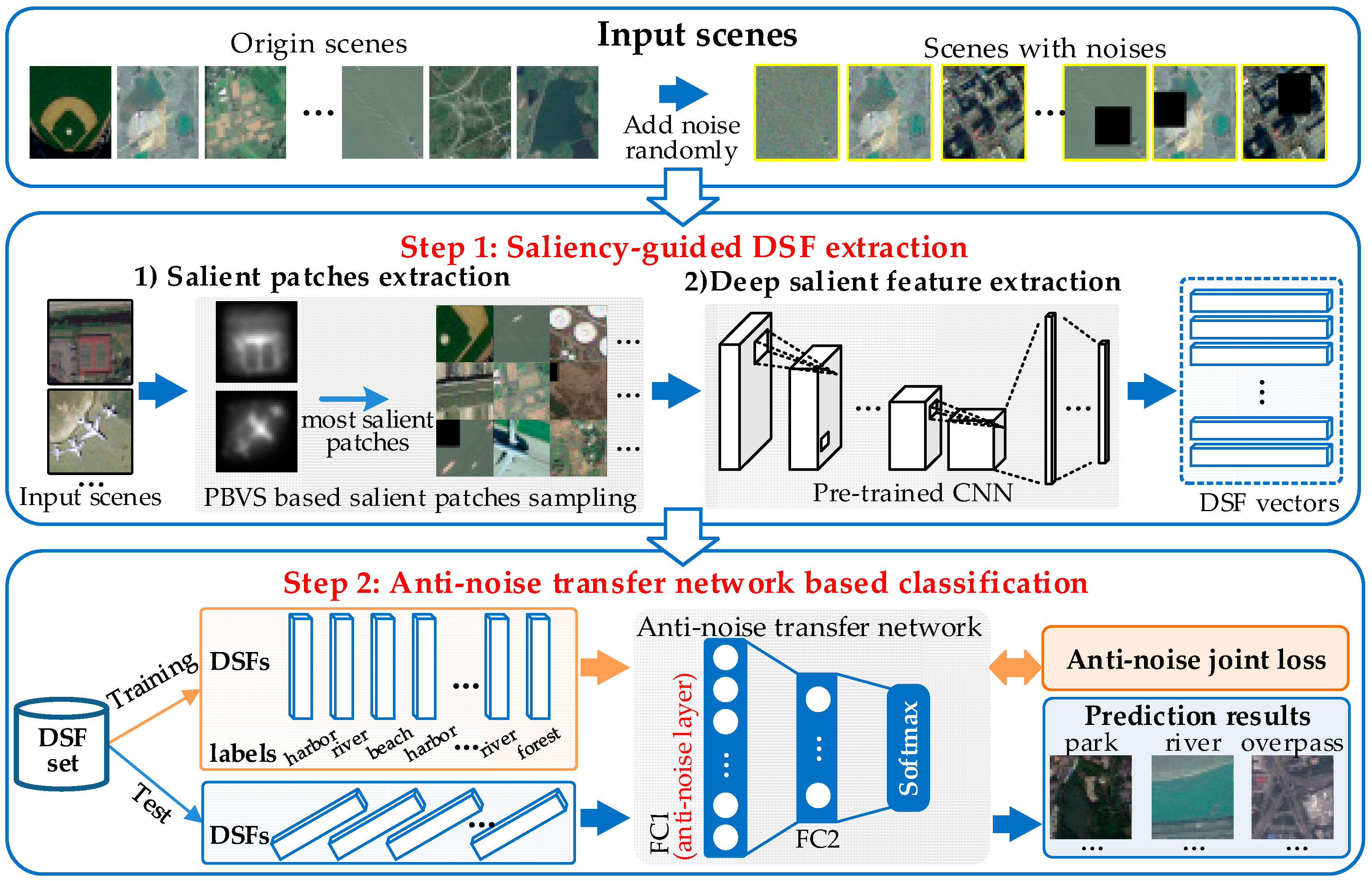
Figure 2.
The flowchart of PBVS based salient patch extraction. The brightness in the saliency map indicates the salient level of the corresponding parts in the input RS scenes: brighter in saliency map, more salient in RS scene. The overlay of RS scene and saliency map make the salient level reflected in the input RS scene, the bigger salient value corresponds higher salient level. The red rectangle is the salient region of the scene.

Figure 3.
The architecture of the very deep CNN with 19 layers (VGG-19)

Figure 4.
The anti-noise transfer network.
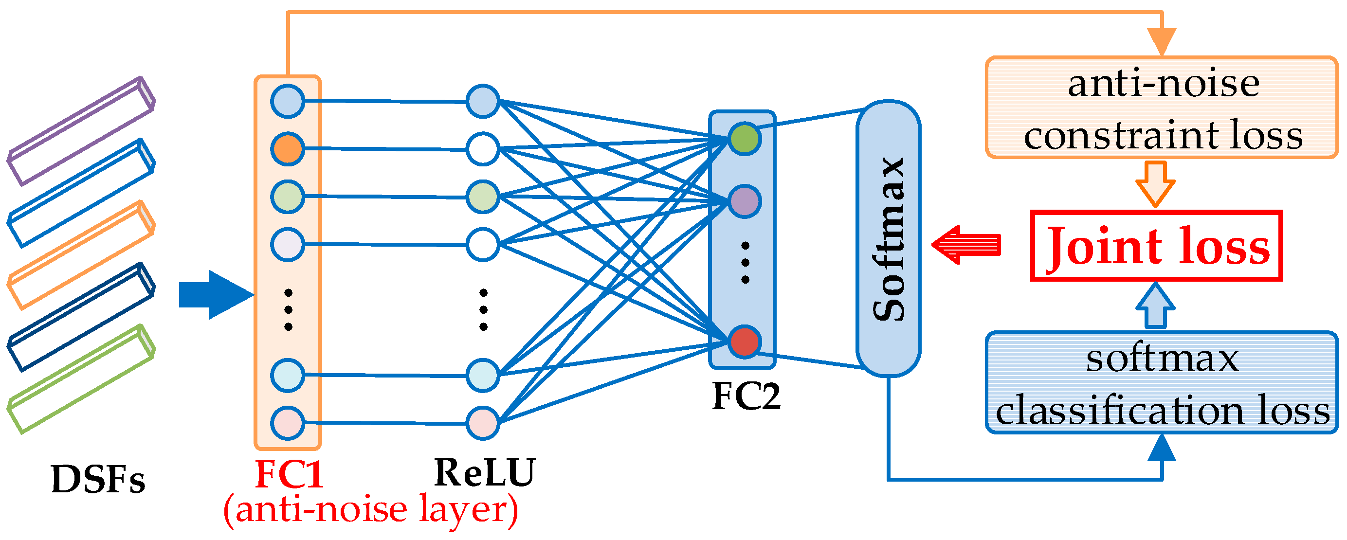
Figure 5.
The categories sequences of the UC Merced Land Use Dataset (UCM), The Google image dataset designed by RS_IDEA Group in Wuhan University (SIRI-WHU) and the SAT-6 dataset: the numbers before the category names will be used to represent the corresponding categories in the experiments.
Figure 5.
The categories sequences of the UC Merced Land Use Dataset (UCM), The Google image dataset designed by RS_IDEA Group in Wuhan University (SIRI-WHU) and the SAT-6 dataset: the numbers before the category names will be used to represent the corresponding categories in the experiments.
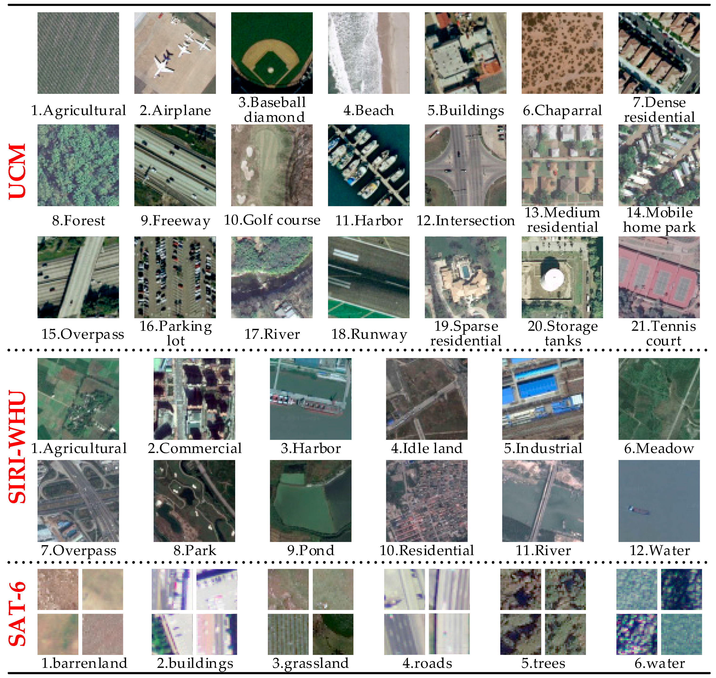
Figure 6.
Confusion matrix of DSFATN on the UCM dataset: the horizontal and vertical axes represent the predict labels and true labels respectively. All categories obtain accuracy higher than 0.96.
Figure 6.
Confusion matrix of DSFATN on the UCM dataset: the horizontal and vertical axes represent the predict labels and true labels respectively. All categories obtain accuracy higher than 0.96.
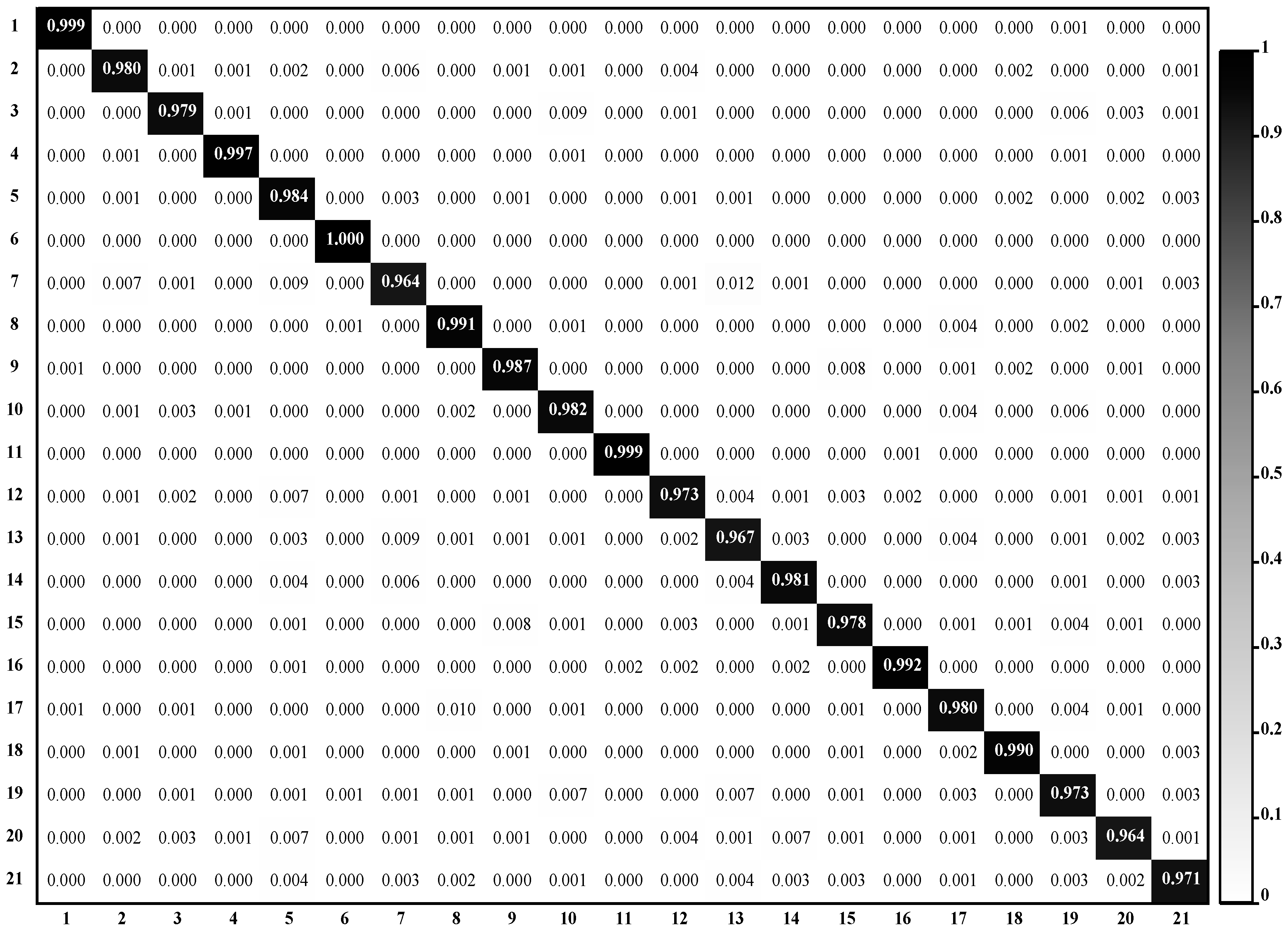
Figure 7.
Confusion matrix of DSFATN on: (a) the SIRI-WHU dataset; and (b) the SAT-6 dataset. The horizontal and vertical axes represent the predict labels and true labels respectively.
Figure 7.
Confusion matrix of DSFATN on: (a) the SIRI-WHU dataset; and (b) the SAT-6 dataset. The horizontal and vertical axes represent the predict labels and true labels respectively.

Figure 8.
The comparison of different features on the three datasets by per-class two-dimensional feature visualization. From left to right: the UCM dataset, the SIRI-WHU dataset and the SAT-6 dataset. From top to bottom: histogram of oriented gradients (HOG), local binary patterns (LBP), scale invariant feature transform (SIFT), CNN(6conv+2fc) feature, and DSF. It is obvious that DSF (the last row) has more clearly separated clusters.
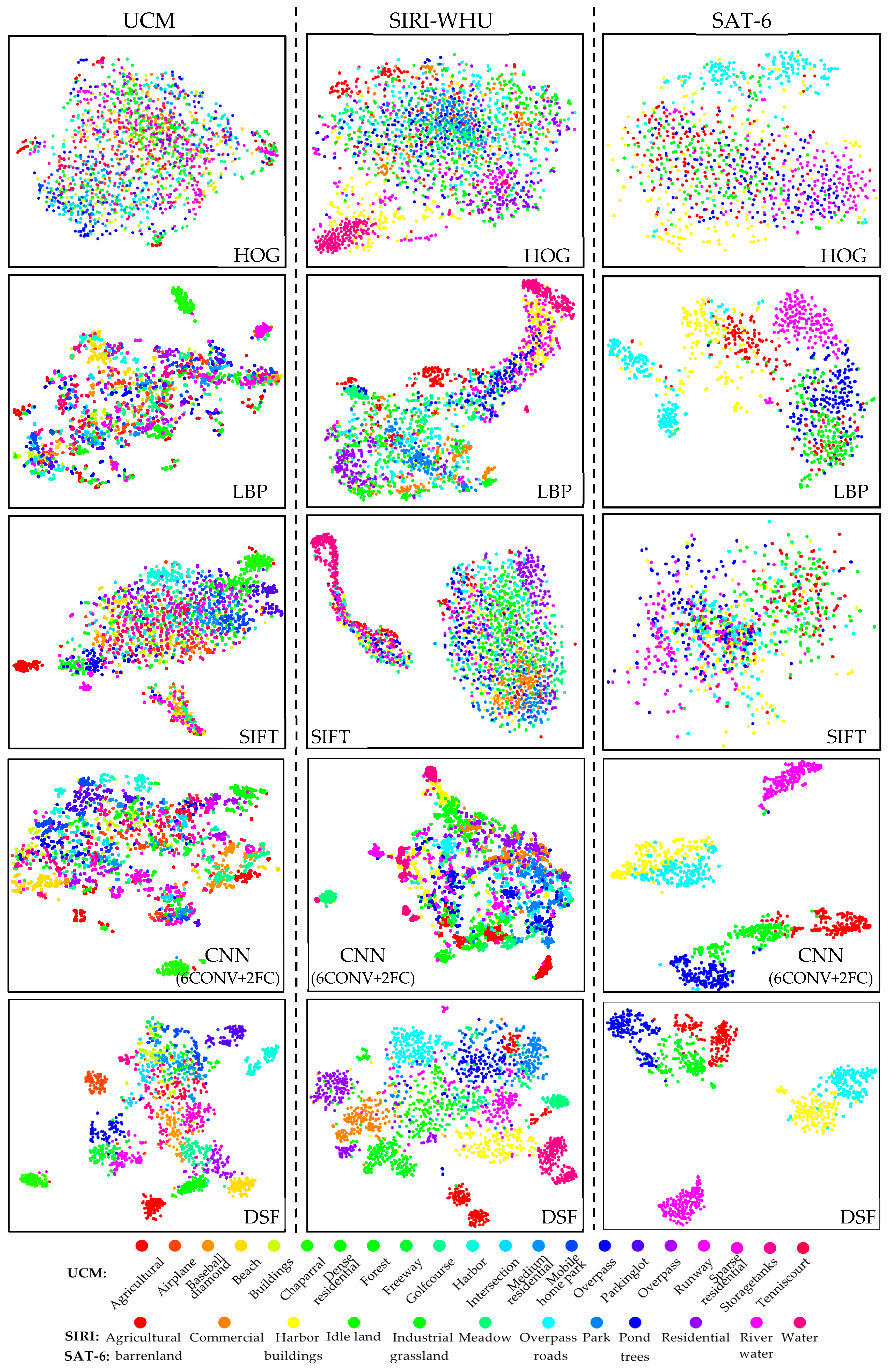
Figure 9.
The per-class accuracy comparisons on: the UCM dataset with salt and pepper noise (top left); the SIRI-WHU dataset with salt and pepper noise (top right); the UCM dataset with partial occlusion (middle left); the SIRI-WHU dataset with partial occlusion (middle right); the UCM dataset with mixed noise (bottom left); and the SIRI-WHU dataset with mixed noise (bottom right). In most cases, the accuracies rank in the following order: DSFATN > TN-2 > TN-1.

Figure 10.
The influence of salient patches’ number α in DSFATN on UCM dataset.

Figure 11.
The influence of the regularization coefficient

Figure 12.
The example scenes of an example tennis court scene at five levels of noise conditions.
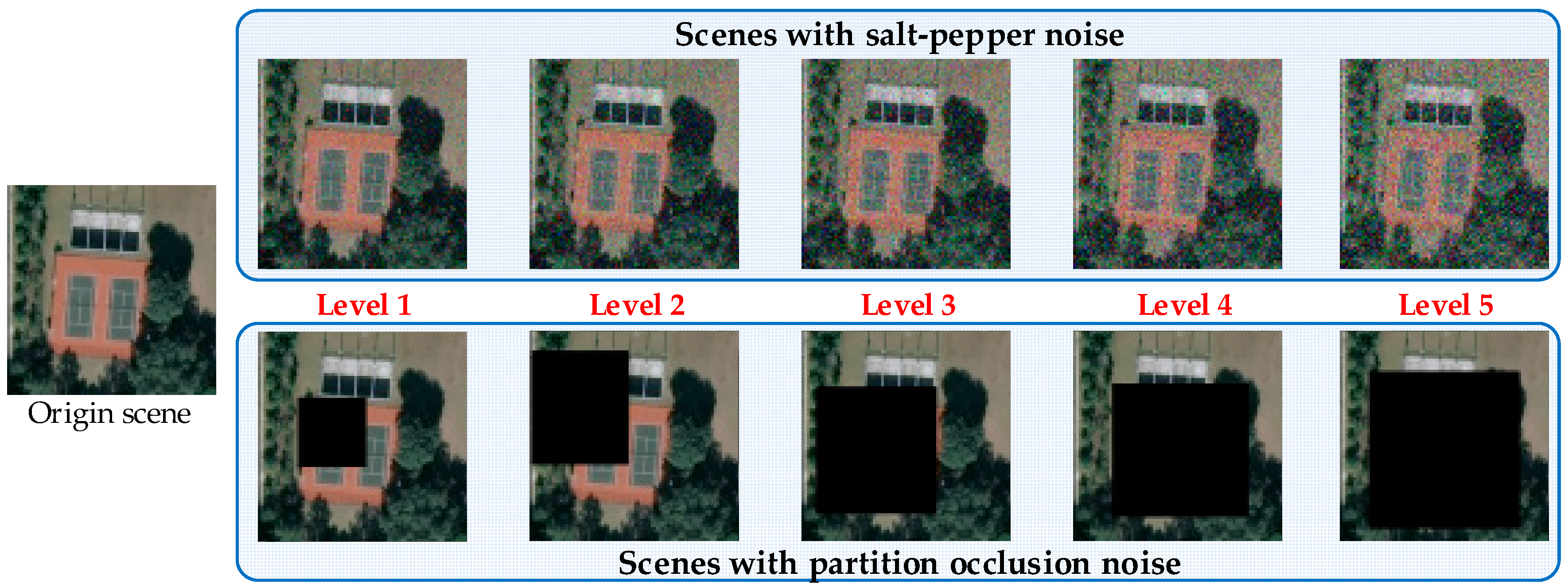
Figure 13.
The results of DSFATN at five levels of noise conditions: the classification accuracies decrease when the noise level increases.
Figure 13.
The results of DSFATN at five levels of noise conditions: the classification accuracies decrease when the noise level increases.

Table 1.
Training and test images’ numbers of the three RS scene datasets.
| UCM | SIRI-WHU | SAT-6 | |
|---|---|---|---|
| Training | 1680 | 1920 | 960 |
| Test | 420 | 480 | 240 |
| Total | 2100 | 2400 | 1200 |
Table 2.
Accuracy comparison of state-of-the-art methods and DSFATN on UCM dataset.
| Rank | Methods | Accuracy (%) |
|---|---|---|
| 1 | RF [49] | 44.77 |
| 2 | CNN(6conv+2fc) | 76.40 |
| 3 | SPCK++ [13] | 77.38 |
| 4 | LDA [15] | 81.92 ± 1.12 |
| 5 | SG + UFL [33] | 82.72 ± 1.18 |
| 6 | PSR [47] | 89.10 |
| 7 | OverFeat [36] | 90.91 ± 1.19 |
| 8 | Caffe-Net [36] | 93.42 ± 1.00 |
| 9 | GoogLeNet [34] | 97.10 |
| 10 | DSFATN | 2 |
Table 3.
Classification results on the SIRI-WHU dataset.
| Methods | RF [49] | LDA [15] | CNN(6conv+2fc) | SPM [12] | DSFATN |
|---|---|---|---|---|---|
| Accuracy (%) | 0 | 60.32 ± 1.20 | 78.20 | 77.69 ± 1.01 | 98.46 |
Table 4.
Classification results on SIRI-WHU dataset.
| Methods | RF [49] | CNN(6conv+2fc) | DeepSat [46] | DSFATN |
|---|---|---|---|---|
| Accuracy (%) | 89.29 | 92.67 | 93.92 | 91.96 |
Table 5.
Classification results on three datasets with different features.
| Features | UCM | SIRI-WHU | SAT-6 | |||
|---|---|---|---|---|---|---|
| Accuracy (%) | Kappa | Accuracy (%) | Kappa | Accuracy (%) | Kappa | |
| Raw image | 33.10 | 0.3361 | 35.83 | 0.3469 | 87.08 | 0.8116 |
| HOG [50] | 52.14 | 0.4975 | 44.79 | 0.3977 | 57.92 | 0.4950 |
| SIFT [51] | 58.33 | 0.5625 | 53.96 | 0.4977 | 45.00 | 0.3400 |
| LBP [52] | 31.43 | 0.2800 | 46.25 | 0.4136 | 77.08 | 0.7250 |
| CNN(6conv+2fc) | 63.10 | 0.6424 | 60.42 | 0.5523 | 94.58 | 0.9188 |
| DSF | 98.07 | 0.9801 | 88.96 | 0.8766 | 96.25 | 0.9437 |
Table 6.
Difference between DSFATN and its variant compared models.
| Model | Multi-Scales Salient Patch Sampling | Anti-Noise Layer Training |
|---|---|---|
| TN-1 | × | × |
| TN-2 | × | √ |
| DSFATN | √ | √ |
Table 7.
Classification results on the UCM dataset and SIRI-WHU dataset with three kinds of noises.
| Model | Classification Accuracy (%) | |||||
|---|---|---|---|---|---|---|
| UCM | SIRI-WHU | |||||
| Salt and Pepper Noise | Partial Occlusion | Mixed Noise | Salt and Pepper Noise | Partial Occlusion | Mixed Noise | |
| RF | 0.0 | 0.0 | 0.0 | 0.0 | 0.0 | |
| CNN(6conv+2fc) | 1.60 | 0.32.00 | 0.380 | 0.460 | 0.5520 | 0.66240 |
| TN-1 | -0.2 | -0.04 | -0.05 | -0.06 | -0.07 | -0.08 |
| TN-2 | -0.4 | 88.76 | 88.33 | 83.83 | 52.1 | 84.79 |
| DSFATN | 0.0 | 0.0 | 0.0 | 0.0 | 0.0 | 0.0 |
Table 8.
Anti-noise analysis on the UCM and SIRI-WHU datasets with different features.
| Features | Classification Accuracy (%) | |||||
|---|---|---|---|---|---|---|
| UCM | SIRI-WHU | |||||
| Salt and Pepper Noise | Partial Occlusion | Mixed Noise | Salt and Pepper Noise | Partial Occlusion | Mixed Noise | |
| HOG [50] | 41.19 | 34.76 | 25.47 | 40.21 | 40.63 | 31.46 |
| SIFT [51] | 62.62 | 41.43 | 44.05 | 51.25 | 46.46 | 46.46 |
| LBP [52] | 25.00 | 18.10 | 10.48 | 37.92 | 39.38 | 25.42 |
| CNN(6conv+2fc) | 56.19 | 38.57 | 47.62 | 52.92 | 65.63 | 53.96 |
| DSF | 89.76 | 83.10 | 82.62 | 79.58 | 87.29 | 83.54 |
| 96.61 | 98.04 | 97.70 | 86.39 | 97.52 | 94.56 | |
Table 9.
Classification results on the UCM dataset with five kinds of scales.
| Models | 25% | 50% | 75% | 100% | 125% | STD |
|---|---|---|---|---|---|---|
| CNN(6conv+2fc) | 76.60 | 80.00 | 77.80 | 76.40 | 80.00 | 1.58 |
| TN-2 | 92.20 | 91.40 | 91.60 | 92.60 | 91.20 | 0.52 |
| DSFATN | 97.87 | 98.53 | 98.46 | 98.25 | 98.22 | 0.23 |
Table 10.
Classification results on the SIRI-WHU dataset with five kinds of scales.
| Models | 25% | 50% | 75% | 100% | 125% | STD |
|---|---|---|---|---|---|---|
| CNN(6conv+2fc) | 77.00 | 77.40 | 77.00 | 78.20 | 75.40 | 0.91 |
| TN-2 | 87.60 | 89.20 | 89.60 | 90.00 | 90.60 | 1.01 |
| DSFATN | 98.30 | 98.39 | 98.73 | 98.46 | 98.92 | 0.23 |
Table 11.
Result comparison with different pre-trained CNNs.
| No. | Pre-Trained CNNs | Classification Accuracy (%) |
|---|---|---|
| 1 | Alexnet [48] | 96.85 |
| 2 | Caffenet [54] | 97.35 |
| 3 | VGG -F [55] | 97.54 |
| 4 | VGG -M [55] | 97.57 |
| 5 | VGG -S [55] | 97.12 |
| 6 | VGG-16 [19] | 97.91 |
| 7 | VGG-19 [19] | 1.4 |
| 8 | Inceptionv1 [35] | 91.25 |
| 9 | Inceptionv2 [56] | 90.54 |
| 10 | Inceptionv3 [57] | 91.82 |
| 11 | Resnetv1_50 [58] | 97.89 |
| 12 | Resnetv1_101 [58] | 97.94 |
Table 12.
The parameters of the salt and pepper noise and partial occlusion at five levels.
| Level | Salt and Pepper Noise Density | Partial Occlusion Covering Scale |
|---|---|---|
| 1 | 0.05 | 10–20% |
| 2 | 0.1 | 20–30% |
| 3 | 0.15 | 30–40% |
| 4 | 0.2 | 40–50% |
| 5 | 0.25 | 50–60% |
© 2018 by the authors. Licensee MDPI, Basel, Switzerland. This article is an open access article distributed under the terms and conditions of the Creative Commons Attribution (CC BY) license (http://creativecommons.org/licenses/by/4.0/).
Share and Cite
MDPI and ACS Style
Gong, X.; Xie, Z.; Liu, Y.; Shi, X.; Zheng, Z. Deep Salient Feature Based Anti-Noise Transfer Network for Scene Classification of Remote Sensing Imagery. Remote Sens. 2018, 10, 410. https://doi.org/10.3390/rs10030410
AMA Style
Gong X, Xie Z, Liu Y, Shi X, Zheng Z. Deep Salient Feature Based Anti-Noise Transfer Network for Scene Classification of Remote Sensing Imagery. Remote Sensing. 2018; 10(3):410. https://doi.org/10.3390/rs10030410
Chicago/Turabian StyleGong, Xi, Zhong Xie, Yuanyuan Liu, Xuguo Shi, and Zhuo Zheng. 2018. "Deep Salient Feature Based Anti-Noise Transfer Network for Scene Classification of Remote Sensing Imagery" Remote Sensing 10, no. 3: 410. https://doi.org/10.3390/rs10030410
Note that from the first issue of 2016, this journal uses article numbers instead of page numbers. See further details here.