Article

Satellite Leaf Area Index: Global Scale Analysis of the Tendencies Per Vegetation Type Over the Last 17 Years

1
CNRM, UMR 3589, Météo France, 42 av Gaspard Coriolis, 31000 Toulouse, France
2
EOLAB, Parc Cientific Universitat de Valencia, C/Catedratico Agustin Escardino, 9, E-46980 Paterna, Valencia, Spain
*
Author to whom correspondence should be addressed.
Remote Sens. 2018, 10(3), 424; https://doi.org/10.3390/rs10030424
Submission received: 23 January 2018 / Revised: 2 March 2018 / Accepted: 6 March 2018 / Published: 9 March 2018

Abstract

:
The main objective of this study is to detect and quantify changes in the vegetation dynamics of each vegetation type at the global scale over the last 17 years. With recent advances in remote sensing techniques, it is now possible to study the Leaf Area Index (LAI) seasonal and interannual variability at the global scale and in a consistent way over the last decades. However, the coarse spatial resolution of these satellite-derived products does not permit distinguishing vegetation types within mixed pixels. Considering only the dominant type per pixel has two main drawbacks: the LAI of the dominant vegetation type is contaminated by spurious signal from other vegetation types and at the global scale, significant areas of individual vegetation types are neglected. In this study, we first developed a Kalman Filtering (KF) approach to disaggregate the satellite-derived LAI from GEOV1 over nine main vegetation types, including grasslands and crops as well as evergreen, broadleaf and coniferous forests. The KF approach permits the separation of distinct LAI values for individual vegetation types that coexist within a pixel. The disaggregated LAI product, called LAI-MC (Multi-Cover), consists of world-wide LAI maps provided every 10 days for each vegetation type over the 1999–2015 period. A trend analysis of the original GEOV1 LAI product and of the disaggregated LAI time series was conducted using the Mann-Kendall test. Resulting trends of the GEOV1 LAI (which accounts for all vegetation types) compare well with previous regional or global studies, showing a greening over a large part of the globe. When considering each vegetation type individually, the largest global trend from LAI-MC is found for coniferous forests (0.0419 m 2 m 2 yr 1 ) followed by summer crops (0.0394 m 2 m 2 yr 1 ), while winter crops and grasslands show the smallest global trends (0.0261 m 2 m 2 yr 1 and 0.0279 m 2 m 2 yr 1 , respectively). The LAI-MC presents contrasting trends among the various vegetation types within the same pixel. For instance, coniferous and broadleaf forests experience a marked greening in the North-East of Europe while crops and grasslands show a browning. In addition, trends from LAI-MC can significantly differ (by up to 50%) from trends obtained with GEOV1 by considering only the dominant vegetation type over each pixel. These results demonstrate the usefulness of the disaggregation method compared to simple ones. LAI-MC may provide a new tool to monitor and quantify tendencies of LAI per vegetation type all over the globe.

Graphical Abstract

1. Introduction

Global environmental change is strongly dependent on land surface processes. Namely, the vegetation dynamics is closely related to the atmosphere through water, CO 2 and energy exchanges [1]. The leaf area index (LAI), defined as the area of green leaves per unit ground horizontal surface area [2,3], is a good indicator of the vegetation growth. As such it is an essential parameter for the description of the vegetation dynamics [4], crop monitoring [5] or climate change studies [6,7]. Nunes, C. and Auge, J.I. [8] reported that LAI can be used for detection of change and for providing information on shifting trends or trajectories in land use and cover change. With recent advances in remote sensing techniques, it has become possible to study the LAI variations at the global scale and in a consistent way over the last decades using a variety of techniques (see, e.g., the review of Fang, H. and Jiang, C. et al. [9]).
How vegetation will respond to climate change has been the topic of several recent studies based on remotely derived LAI. Most of them reported positive trends in vegetation (greening) during recent decades [10,11,12,13,14,15]. In return, changes in vegetation dynamics may affect local climate via several biophysical processes, leading to positive or negative feedback in the land-climate system [16,17]. For instance, Forzieri, G. et al. [18] showed that positive trend in LAI contributed to the warming of boreal zones and to a cooling in arid regions. The impacts of climate change on the vegetation dynamics and their potential interactions have been increasingly studied, given their possible benefits in carbon sequestration [19,20,21].
Zhu, Z. et al. [14] related changes in vegetation greenness to multiple biogeochemical drivers (such as CO 2 concentration in the atmosphere or changes in temperature and precipitation) and land-use effects (fertilization, irrigation, etc.). They also identified local impact at regional scale of such drivers on the vegetation dynamics. For instance, rising CO 2 is the dominant factor in the tropical zone while changes in the vegetation dynamics are mainly driven by climate warming in high latitudes of the Northern Hemisphere.
Vegetation growth highly depends on climate conditions but also on the vegetation coverage density (sparsely, moderately or highly vegetated regions), as shown by Feng, H. et al. [22]. In addition, the type of vegetation is expected to play a role in the relationship between vegetation and climate as the growing mechanisms of the plant differ from one type to another (e.g., drought avoiding or drought tolerant behaviours for crops, [23]). There is a quite extensive literature on the recent greening of different vegetation types, including forests (e.g., [16,19,24,25]) and grasslands (e.g., [18,26,27,28]).
These studies were based on land cover maps to select pixels or areas corresponding to a specific vegetation type. Land cover maps describe the partition of land surfaces into several biomes depending on their seasonal vegetation cycle. These maps generally provide, at high spatial resolution, either one type of vegetation (or plant functional type, PFT) per pixel (e.g., ESA-CCI Land Cover, [29]), or cover fractions of several PFTs per pixel (e.g., ECOCLIMAP-II, [30]). In both cases, assigning only one vegetation type per pixel, generally the dominant one, has two main drawbacks. First the LAI supposed to represent the dominant vegetation type is contaminated by spurious signal due to other types. Second, at the global scale, significant areas of each vegetation type are neglected. Figure 1 presents the fraction of the vegetated area (bare soil excluded) corresponding to the dominant vegetation type based on the ECOCLIMAP-II land cover map at 5 km resolution. Some regions in the world show values very close to 1, meaning that these areas are very homogeneous (only one vegetation type within the pixel), like the Amazon forest or the Tibetan plateau for instance. However, in most parts of the globe, pixels at this resolution are mixed and the signal is not necessarily representative of the dominant vegetation type. At this resolution, 12% of the total grassland area, 23% for evergreen forests, 36% for coniferous forests and 72% of broadleaf forests are neglected. In the following, the method that consists in selecting only the dominant vegetation type for each pixel will be referred as the single-dominant selection method.
Retrieving the LAI of each vegetation type within a pixel from the total observed LAI is not straightforward. Because these products present a coarse spatial resolution (e.g., 1 km for GEOV1, [31]), the spatial scale does not permit discriminating between vegetation types within mixed pixels. The observed LAI over a pixel represents the weighted average of LAI of each type of vegetation within the pixel. Thus, despite the importance of improving our understanding of vegetation dynamics and its relationship with climate change, the mechanisms driving the vegetation growth are still unclear [32].
In a previous study, Carrer, D. et al. [33] presented an innovative method to disaggregate satellite-based albedo into bare soil and vegetation albedos. They developed a Kalman Filter (KF) approach to retrieve both quantities from a decade of MODIS data on a global scale. The derived product showed good agreement with previous studies and was indirectly assessed through the relationship between bare soil albedo and soil moisture. The method was further improved by Planque, C. et al. [34] to include a dynamic fraction of vegetated area into the retrieval.
The main objective of this study is to detect and quantify changes in the vegetation dynamics for individual vegetation type at the global scale over the last 17 years. Following the method of Carrer, D. et al. [33], we first develop a Kalman Filter approach to disaggregate the satellite-derived LAI from GEOV1 over nine main vegetation types, including broadleaf, coniferous and evergreen forests as well as crops and grasslands. We use data from the ECOCLIMAP-II land cover database as prior information. This KF approach permits the separation the individual LAI of different vegetation types that co-exist in a grid pixel. In a second step a trend analysis is conducted using a statistical test for each vegetation type over the 1999–2015 period. The analysis is performed at both global and regional scales (continental scale and main climate zones).
Section 2 presents the GEOV1-LAI satellite product and the ECOCLIMAP-II database, as well as in situ LAI observations used for validation purposes. The disaggregation method based on the KF is detailed in Section 3. Validation against in situ observation and trend analysis are presented in Section 4 and discussed in Section 5.

2. Material

2.1. Satellite-Based Leaf Area Index

Different methods were proposed to retrieve biophysical variables, including LAI (see e.g., [35]). Our analysis relies on LAI from the GEOV1 dataset [31] provided by the Copernicus Global Land Service (http://land.copernicus.eu/global). It consists of 1 km × 1 km global maps of LAI provided every 10 days using a 30-day temporal window. This product is derived from SPOT/VEGETATION (from 1999 to 2014) and PROBA-V (from 2014 to present) observations using an Artificial Neural Network trained by fused MODIS-15 [36] and CYCLOPES [37] products. It has to be noted that the MODIS LAI retrieval is based on biome-specific Lookup Tables while the other LAI satellite products do not consider any biome specification. This could introduce biases in the GEOV1 LAI product which is assumed to represent, for each 1 km pixel, an aggregated LAI value. Another source of potential biases comes from the different assumptions on the canopy architecture used in the CYCLOPES and MODIS retrievals. The GEOV1 LAI products will thus be relatively consistent with an effective LAI for low LAI values and closer to the actual LAI for high values [38].
Nevertheless, Camacho, F. et al. [39] demonstrated the reliability of GEOV1 to represent the LAI, namely in terms of spatial and temporal consistency. The authors compared the GEOV1 product with other satellite-based datasets and found better performances with GEOV1 compared to ground measurements over different regions of the globe and various vegetation types. Fang, H. et al. [9] presented an intercomparison of five global LAI products including GEOV1. They reported that GEOV1 is globally consistent with other products ( R 2 > 0.74 ) and that it presents satisfactory uncertainties for different biome types (0.24 m 2 m 2 on average). Finally, Camacho, F. et al. [40] studied the consistency between the LAI derived from both SPOT/VEGETATION and PROBA-V. They found a high degree of consistency, which justifies their use for trend analyses.
GEOV1 is provided with quality flags that were used in this study to remove pixels with snow and those contaminated by clouds. To reduce the computation costs and storage volume, the product was resampled at a spatial resolution of 1/20 degree. This resampling significantly reduces the total storage volume of the final disaggregated product from about 7 To to 200 Go. Moreover, we can assume that the resampling partly reduces the potential bias introduced by the biome-specification in the MODIS retrieval. Figure 2 shows the mean GEOV1 LAI averaged over the 17-year period of this study.

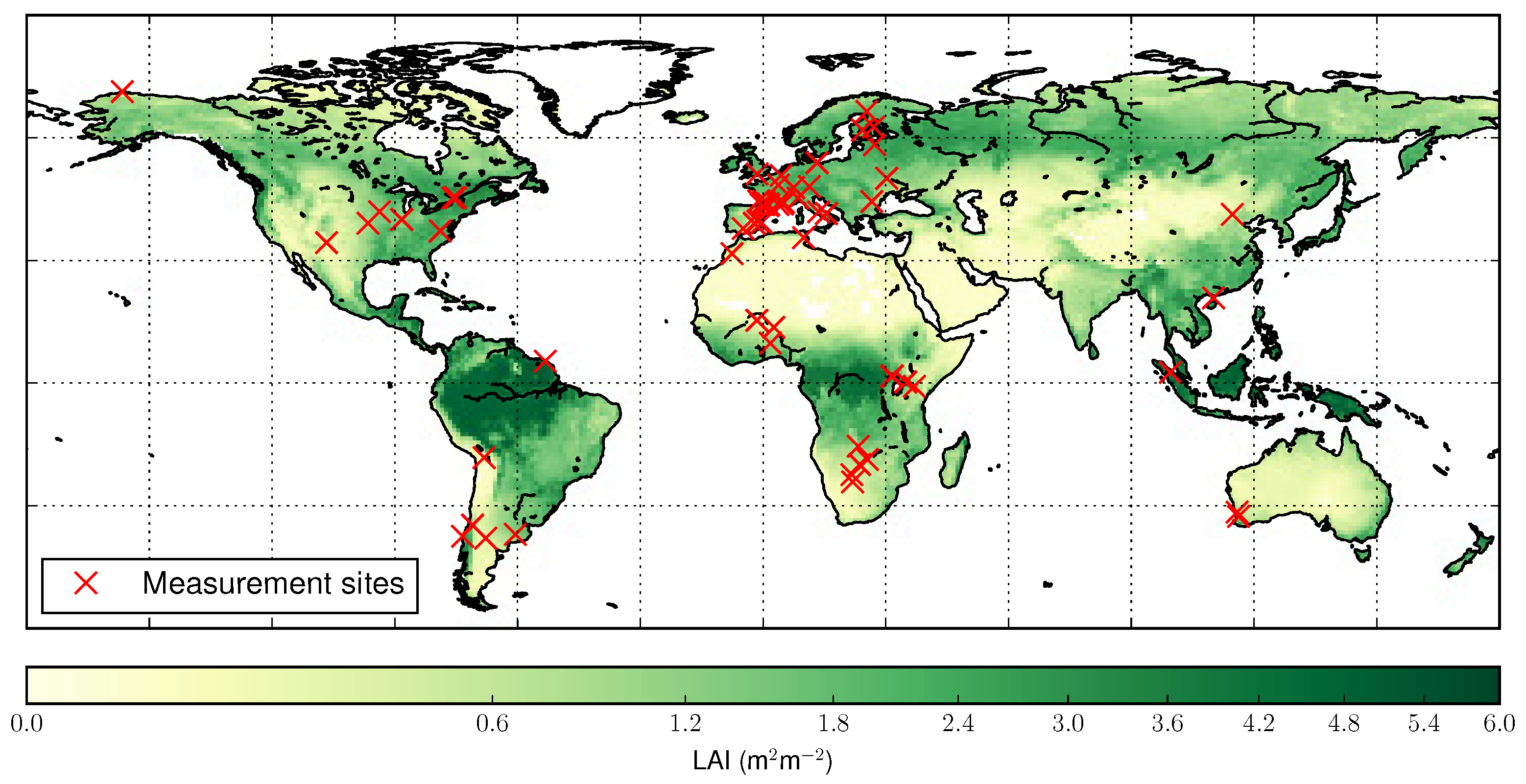
2.2. In Situ Leaf Area Index

LAI ground measurements are coming from the Direct2.0 database provided by EOLAB. Direct2.0 is the second version of the Direct database of the CEOS cal/val OLIVE (On line Validation Exercise) tool [41]. Direct2.0 includes a selection of Direct sites [39] plus additional sites coming from FP7 ImagineS project [42]. Direct sites were originally compiled by Garrigues, S. et al. [43] from different initiatives such as VALERI (http://w3.avignon.inra.fr/valeri), BigFoot [44], NASA (SAFARI-2000; [45]), Boston University [46], Canada Centre for Remote Sensing [47], US Environmental Protection Agency [48] and ESA covering the period 2000–2010. Actual LAI ground estimates were mainly collected with devices like TRAC [49] or Digital Hemispherical Photos [50], which are able to estimate the clumping index [51] to correct the effective LAI value for the non-randomness distribution of leaves. Camacho, F. et al. [39] screened out the potential sources of uncertainties primarily affecting ground estimates from indirect techniques. As a result, a total of 30 forest sites where the understory was not measured were discarded for accuracy assessment due to the important contribution of the understory to the total canopy LAI observed from the space. The FP7 ImagineS ground database was recently delivered (http://www.fp7-imagines.eu/), and includes ground measurements over a network of 20 sites, mostly croplands. A total of 44 new ground-based LAI maps were produced during the period 2013–2016 [42], leading to 83 sites used in this study (location shown in Figure 2). Ground LAI values were estimated from DHP measurements and processed with the CAN-EYE software [52]. More details on the description of sites can be found in Camacho, F. et al. [39] for Direct Sites and in Camacho, F. et al. [42] for ImagineS Sites.
In both databases, Direct and ImagineS, the in situ data was collected and up-scaled according to the guidelines defined by the CEOS/WGCV LPV subgroup [53,54]. The direct validation approach consists in using high spatial resolution imagery (such as Landsat-7/ETM+, Landsat-8/OLI, SPOT-4/HRVIR and SPOT-5/HRG) to scale the local ground measurements up to the 3 × 3 km 2 area of the site. The RMSE of the fine-resolution LAI estimate is typically ranging between 0.5 and 1 m 2 m 2 [42]. An empirical “transfer function” between the high spatial resolution radiometric signal and the biophysical measurements is established using a representative number (between 30 and 50) of elementary sampling units (ESUs) which are distributed among the different main land cover types of the study area (e.g., [55,56]). The transfer function is then applied to all the high spatial resolution pixels of the whole site. The resulting high spatial resolution map of the considered biophysical variable is finally averaged over the 3 × 3 km 2 to get the average values which are used for the validation of satellite products. For the comparison of ground measurements with satellite products (Section 4.2), ground measurements are supposed to represent the LAI of one specific vegetation type over a 1/20 degree pixel.

2.3. ECOCLIMAP-II Land Cover Database

ECOCLIMAP-II [30] is a global land cover map gathering bio-geophysical parameters of 520 ecosystems at a resolution of 1 km. It was initially designed to provide Land Surface Models (LSMs) such as ISBA (Interactions between Soil, Biosphere, and Atmosphere [57]) within the SURFEX platform (SURFace Externalisée, [58]) with vegetation and soil parameters, including LAI, fractional vegetation cover, albedo, soil depth, etc. ECOCLIMAP-II is currently used by Météo-France for climate and Numerical Weather Prediction modeling.
ECOCLIMAP-II provides LAI seasonal cycle for each vegetation type. These estimates are based on MODIS LAI temporal maps at 1 km resolution and covering the 2000–2005 period. A simple disaggregation method (based on the search of homogeneous neighbouring pixels) was used to disentangle the contribution of each PFT and establish the LAI seasonal variations. A full description of the ECOCLIMAP-II database is available in Faroux, S. et al. [30]. No deep uncertainty analysis on LAI climatology was performed, but the consistency of LAI and fraction of vegetation was checked by Faroux, S. et al. [30] after broad-scale aggregation.
To match different spatial resolutions as well as the vegetation types represented by the different LSMs, ECOCLIMAP-II can be aggregated to provide merged multi-ecosystem physiographic information for each cover (or vegetation type). Here 12 covers (default configuration of SURFEX) are considered: 3 covers without vegetation (bare soil, open water and snow), and 9 vegetation covers (broadleaf forest, coniferous forest, evergreen forest, summer crops, winter crops, irrigated crops, grassland, tropical grassland and wetland). In the following, winter crops and irrigated crops are merged, as well as grasslands and tropical grasslands. The wetland cover was discarded because its fraction is very small all over the globe. Global maps of the cover fraction of the six vegetation types are shown in Figures S1–S2.

3. Method

3.1. Development of the LAI Multi-Cover
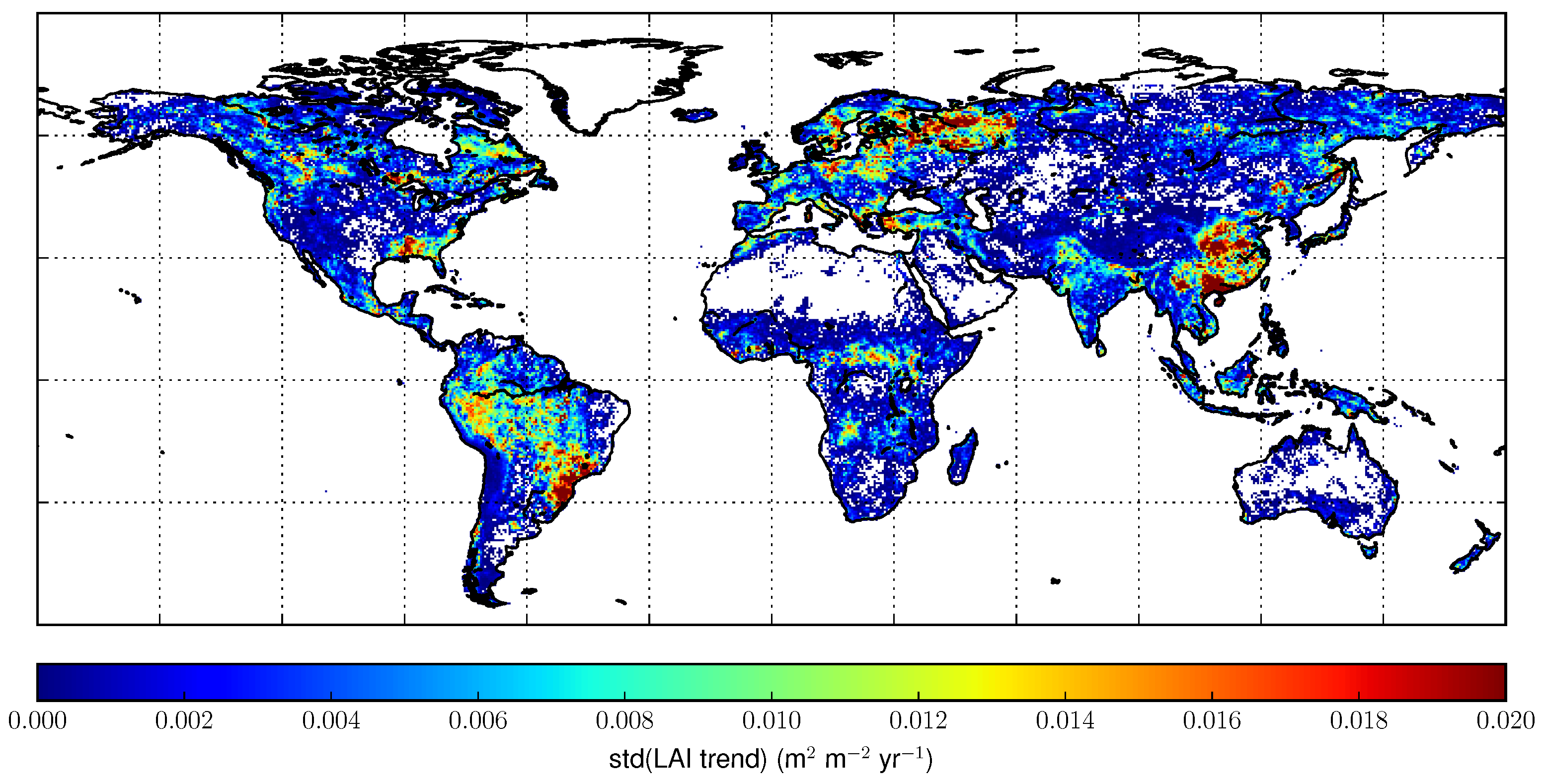
The algorithm to disaggregate the GEOV1 LAI relies on a KF approach. The KF is a sequential data assimilation technique which aims at correcting the state of a model from observations by minimizing the error variance.
Here, the state vector embeds the LAI of the 12 considered covers:
X = LA I 1 , , LA I 12 T
Besides, the LAI is assumed to vary slowly at the 10-day temporal scale. Hence the background state X b ( k ) at a given time step k corresponds to the analyzed state X a ( k 1 ) at the previous time step (persistence hypothesis) , where superscripts a and b stand for analysis and background (guess), respectively. The LAI seasonal cycle of each cover provided by ECOCLIMAP-II is used to constrain the partitioning of the total LAI from GEOV1 and is then included into the observation vector:
Y ( k ) = LA I 1 E C O ( k ) , , LA I 12 E C O ( k ) , LA I S A T ( k ) T
where LA I j E C O is the LAI from ECOCLIMAP-II for cover j and LA I S A T is the total LAI from GEOV1.
The analysis equations of the KF is then written as:
X a = X b + K Y H X b
A a = I K H A b
where H is the observation operator, K the Kalman gain matrix, A the state error covariance matrix and I the identity matrix.
The total LAI can be computed as the average of the LAI of each cover weighted by the fraction f j ( j = 1 , , 12 ) of each cover within the pixel. The observation operator H is then given by:
H = 1 0 0 1 f 1 f 12
The Kalman gain depends on the observation error covariance matrix R and is given by:
K = A H T H A H T + R 1
The error covariance matrix R depicts the uncertainty of the GEOV1 satellite product and of the ECOCLIMAP-II LAI seasonal cycle, as well as the error correlation between both. When assuming that the observations are independent of the climatological parameters from ECOCLIMAP-II, it comes:
R = σ 1 E C O 2 0 σ 12 E C O 2 0 σ S A T 2
The GEOV1 product is provided with a quantitative estimation of the uncertainty which could have been used to set up σ S A T . However, ECOCLIMAP-II only provides the LAI seasonal cycle for each cover type and is mainly used here to inform the algorithm on the potential partitioning of LAI among the cover types. Considering that the KF accounts for relative uncertainties, the uncertainty σ j E C O of the climatological parameters should then be constantly greater than σ S A T . Consequently, σ j E C O was set to 10 times σ S A T .
The Kalman gain also accounts for errors in the prognostic state via matrix A. The latter encompasses all model uncertainties, which are assumed to be normally distributed with zero mean and covariance Q. The model states are assumed independent and matrix Q is then diagonal. Under the persistence assumption, the forecast error covariance A b is given by:
A b ( k ) = A a ( k 1 ) + Q
As proposed by Cedilnik, J. et al. [59], the model error covariance matrix Q is set proportional to the analysis error covariance matrix A a ( k 1 ) with a coefficient equal to the cover fraction f j . This gives more uncertainties to less dominant covers. Also, the state uncertainties are inflated by α = 50 % over a 10-day period. Hence, the diagonal terms of A b ( k ) = a i j b ( k ) which represent the modeled LAI uncertainties for each cover are given by:
a j j b ( k ) = ( 1 + α ) ( 1 + f j ) a j j a ( k 1 )
At time steps where no observation is available, the uncertainty σ S A T of the satellite observation in matrix R is given a large value. As a consequence, there is no more constraint on the total LAI in the KF process and the LAI of each cover converges toward the corresponding value from ECOCLIMAP-II. The convergence speed directly depends on the inflation of the state uncertainties in matrix A. Since the total LAI from ECOCLIMAP-II may significantly differ from the satellite observations, this causes some unrealistic variations in the analyzed LAI. Thus, the analyzed LAI of each cover is considered to be a missing value when no observation is available.
The derived product, called LAI-MC (Multi-Cover), then consists of world-wide LAI maps at a spatial resolution of 1/20 degree provided every 10 days for each vegetation type over the period 1999–2015.

3.2. Trend Analysis

We used the non-parametric Mann-Kendall (MK) test [60] to investigate the trends in vegetation dynamics (greening/browning) for each cover independently. The MK test has been widely used to detect significant trends in climatic and environmental parameters (e.g., [14,15]).
The MK test being sensitive to the signal seasonality, the LAI of each vegetation type was first averaged over each year at the pixel scale. A significance level of 0.01 was used to reject the null hypothesis of the MK test and detect significant trends. When a significant trend was detected, the Sen’s Slope test was used to quantify the trend [61].

4. Results

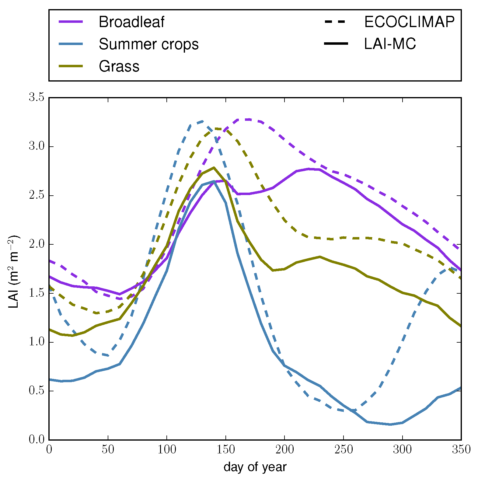
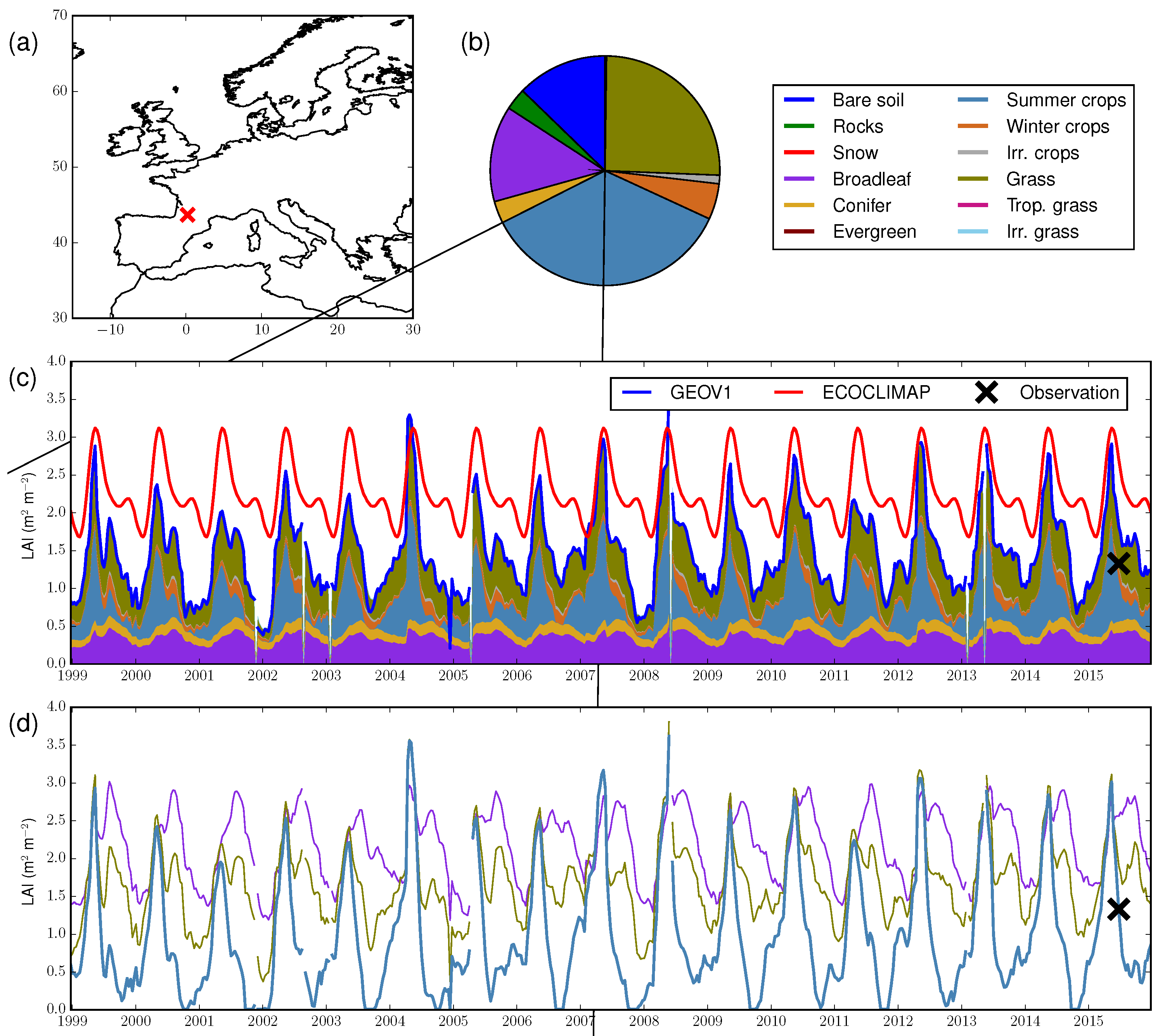
4.1. Illustration at One Location

To illustrate the partitioning of the total LAI from GEOV1 over the 9 vegetation types, we plotted several time series of LAI for one specific site where a ground observation is available, located South-West of France (Figure 3a). The fractions of each of the 12 covers from ECOCLIMAP-II are shown in Figure 3b. LAI is not computed for the first three covers since they represent bare soil, rocks and snow, respectively. For this pixel, summer crops is the dominant vegetation type (36%), followed by grasslands (25%) and broadleaf trees (14%). The total LAI from ECOCLIMAP-II is shown in red in Figure 3c. Since ECOCLIMAP-II only provides climatological values, the red curve does not show any interannual variability. At this location, ECOCLIMAP-II clearly overestimates LAI compared to GEOV1 (blue curve), especially during the low-vegetation periods. On the other hand, the seasonal cycles are fairly consistent. Figure 3d shows the LAI time series for the three dominant vegetation types obtained with the disaggregation algorithm (LAI-MC), while their respective contribution to the total LAI is represented by colored patches in Figure 3c. The amplitude and phase differ from one PFT to another, which is due to (1) different seasonal cycles from ECOCLIMAP-II and (2) the dynamical behaviour of the algorithm. The summer crops show the highest amplitude, with almost null values during the winter. The amplitude and phase of both grasslands and broadleaf trees are quite similar, but broadleaf trees show higher LAI values.
Figure 4 presents the seasonal cycle of the LAI from ECOCLIMAP-II and LAI-MC for the three main PFTs. The values from ECOCLIMAP-II shown by the dashed lines were used as prior information in the Kalman Filter via Equations (2) and (3). They basically helped the algorithm to partition the total satellite-derived LAI across PFTs. Since the KF is a sequential algorithm that propagates states and errors through time, the partitioning of the total LAI can evolve in time. As a consequence, the seasonal cycle of LAI-MC and ECOCLIMAP-II may differ, which can be seen in Figure 4. For instance, the LAI of summer crops from LAI-MC is greater than from ECOCLIMAP-II during a part of the autumn while it is lower for broadleaf trees and grasslands. In addition, ECOCLIMAP-II shows a second growing phase for summer crops during winter, which is not reproduced in LAI-MC. On the other hand, the main peak of summer crops during the summer is well captured but it partly affects the other PFTs, namely broadleaf trees which reach their peak one or two months later in the ECOCLIMAP-II database.

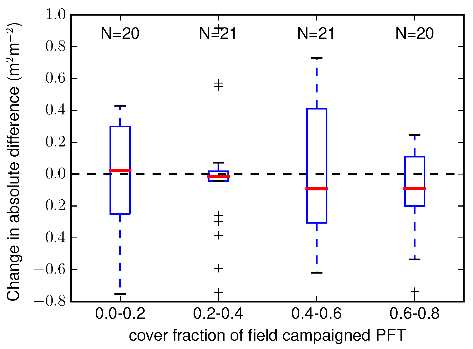
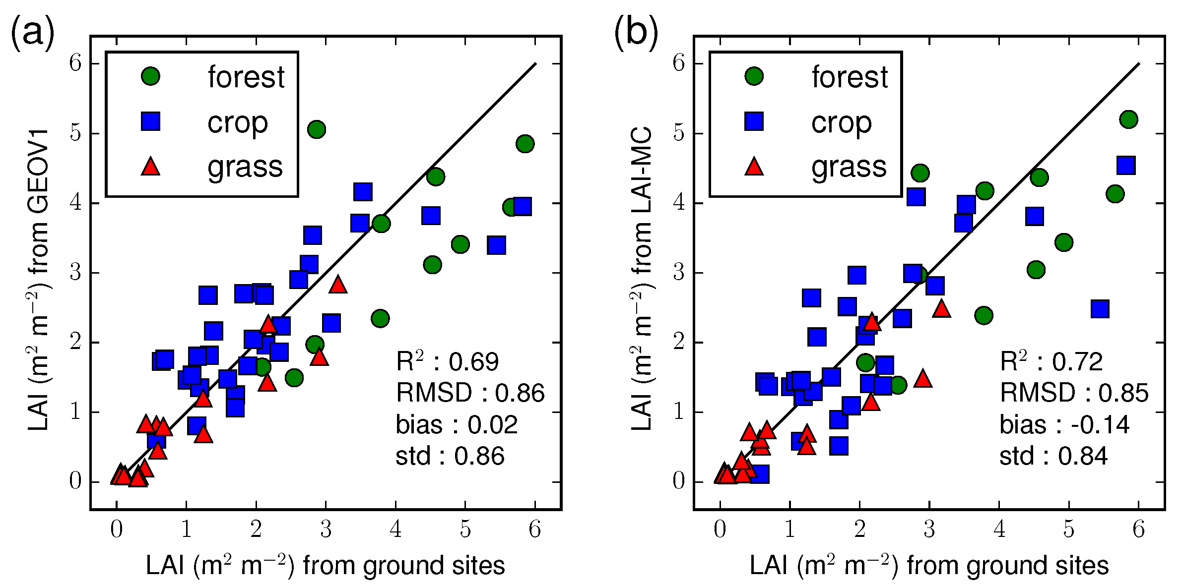
4.2. Validation Against Ground Observations

Figure 3c,d show one ground observation for this site on 23 June 2015 (black cross). Compared to the ground observation, GEOV1 overestimates LAI (1.83 m 2 m 2 for GEOV1 and 1.33 m 2 m 2 for the ground observation). For this site, the ground observation was made in a crop field so the measurement has to be compared to the LAI of summer crop in the LAI-MC product (blue line), which equals 1.31 m 2 m 2 for this date. In that case, LAI-MC matches the ground observation very well.
A total number of 91 values of ground observations were collected over 83 sites. For each site, the type of vegetation is given (among forest, crop and grassland) and an ECOCLIMAP-II PFT is attributed accordingly. LAI from LAI-MC in the corresponding PFT is compared to the ground observations (it is reminded that LAI-MC provides, for each pixel, LAI values for each vegetation type). The comparison is also done with the original GEOV1 product, which represents the mean LAI of the pixel, across vegetation types. Results are shown in Figure 5. Quantitative scores, including correlation (R 2 ), Root Mean Square Difference (RMSD), bias and standard deviation (std) are indicated in Table 1. When considering all sites, scores of LAI-MC are slightly better than those of GEOV1, except for the bias (0.02 m 2 m 2 and −0.14 m 2 m 2 for GEOV1 and LAI-MC, respectively).
Looking into more details, the best improvements from GEOV1 to LAI-MC are shown over forest sites which, also, show the largest discrepancies between satellite-derived products and ground-based observations. For the crop sites, the bias is significantly smaller with LAI-MC (−0.03 m 2 m 2 ) than with the native GEOV1 product (0.22 m 2 m 2 ). On the contrary the LAI scores over grassland sites is slightly worse for LAI-MC.
Figure 6 presents the change in absolute differences with ground observation from GEOV1 to LAI-MC with respect to the cover fraction of the vegetation type corresponding to each site. In this figure, ground sites are classified according to the cover fraction of the PFT over which in situ measurements were made. This is a first order estimate of the vegetation heterogeneity. When the cover fraction is large (close to 1), the pixel is quite homogeneous. On the other hand, when the cover fraction of the measured biome is small, the pixel can be quite homogeneous (if there is only one other biome) or heterogeneous (if there are multiple biomes with small cover fractions). On average, there is little difference between GEOV1 and LAI-MC when the cover fraction is small (lower than 0.4). On the other hand, LAI-MC is closer to the ground observations when the cover fraction is greater than 0.4. In Section 3, it is stated that higher uncertainty is given to less dominant covers in the disaggregation process. This reflects the fact that PFTs with small cover fractions only slightly impacts the averaged LAI as observed by GEOV1, and is then more difficult to retrieve. To conclude, Figure 6 shows that, on average, LAI-MC performs better than GEOV1 for PFTs with non-negligible cover fractions (0.4 to 0.8) but does not improve the LAI retrieval for PFTs with small cover fractions. Nevertheless, we can suppose that the higher uncertainties for PFTs with small cover fractions do not significantly impact LAI trends when spatially averaged since spatial averages are weighted by the cover fraction to represent the effective area of each vegetation type.
Validating products from satellite observations against ground-based observations largely relies on the representativeness of the local site over the pixel seen by the satellites. This validation exercise shows some discrepancies between LAI-MC and ground observations, but the scores are quite good, and at least as good as for the original GEOV1 product, even for pixels where the vegetation type corresponding to the ground observation is not dominant (see Figure 6). The great advantage of LAI-MC compared to the GEOV1 product is that it provides LAI values for all the vegetation types present in the pixel.

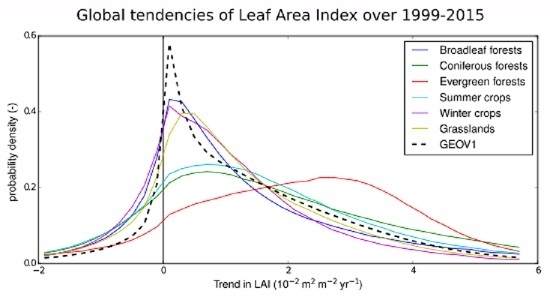
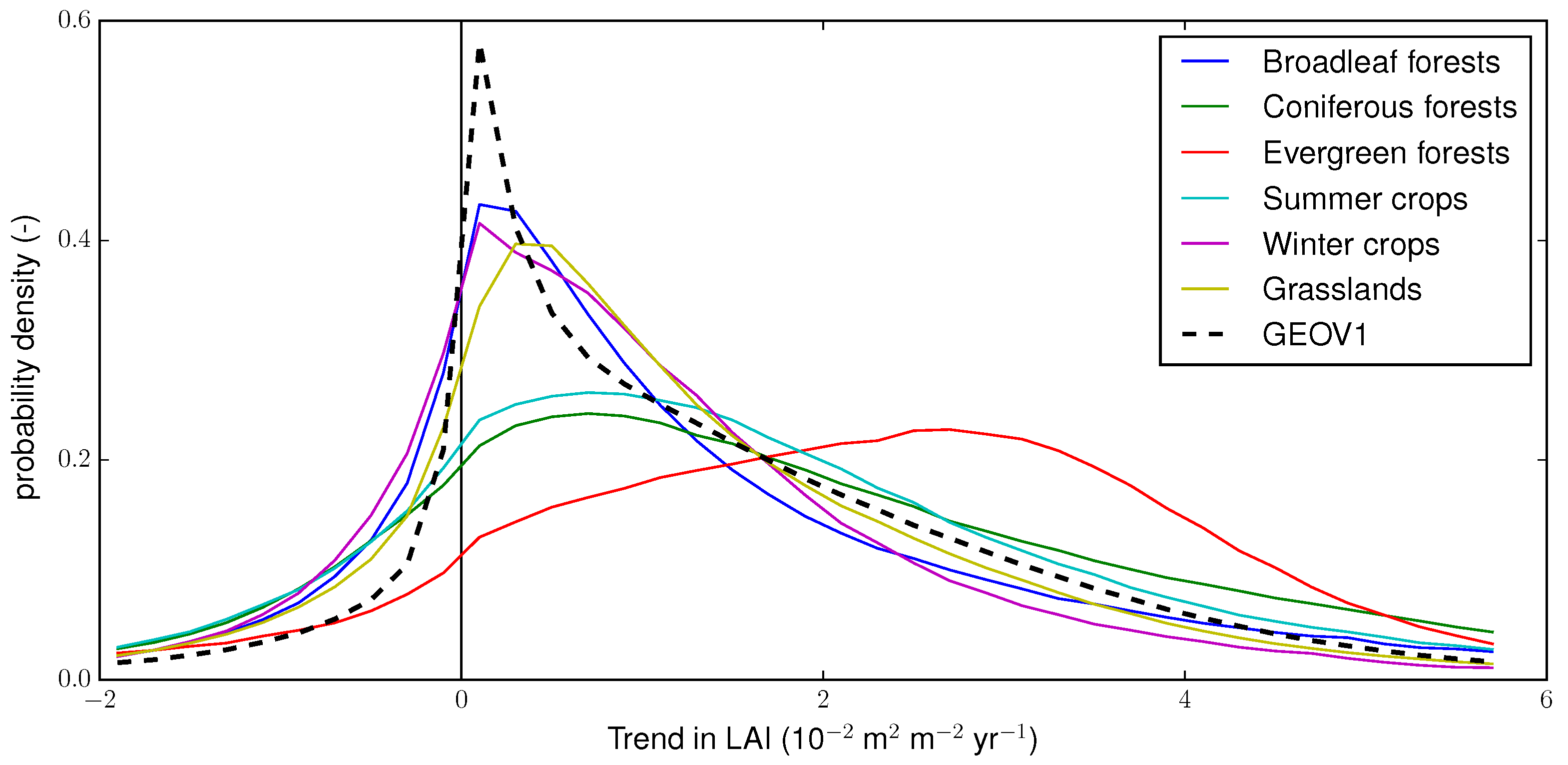
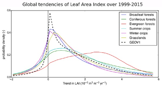
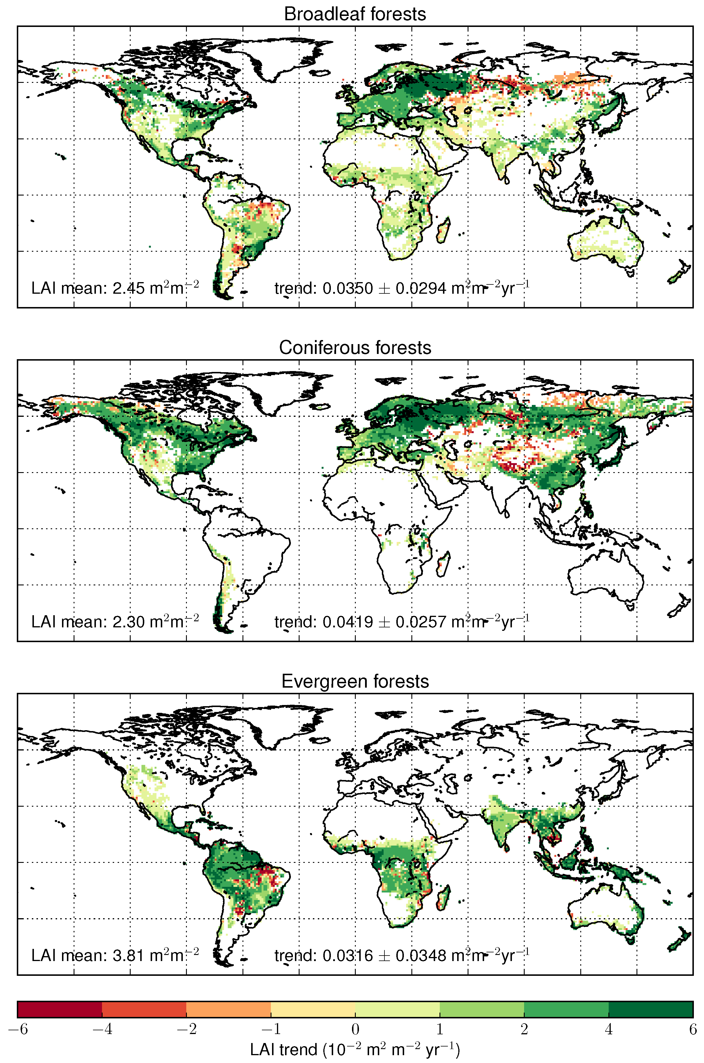
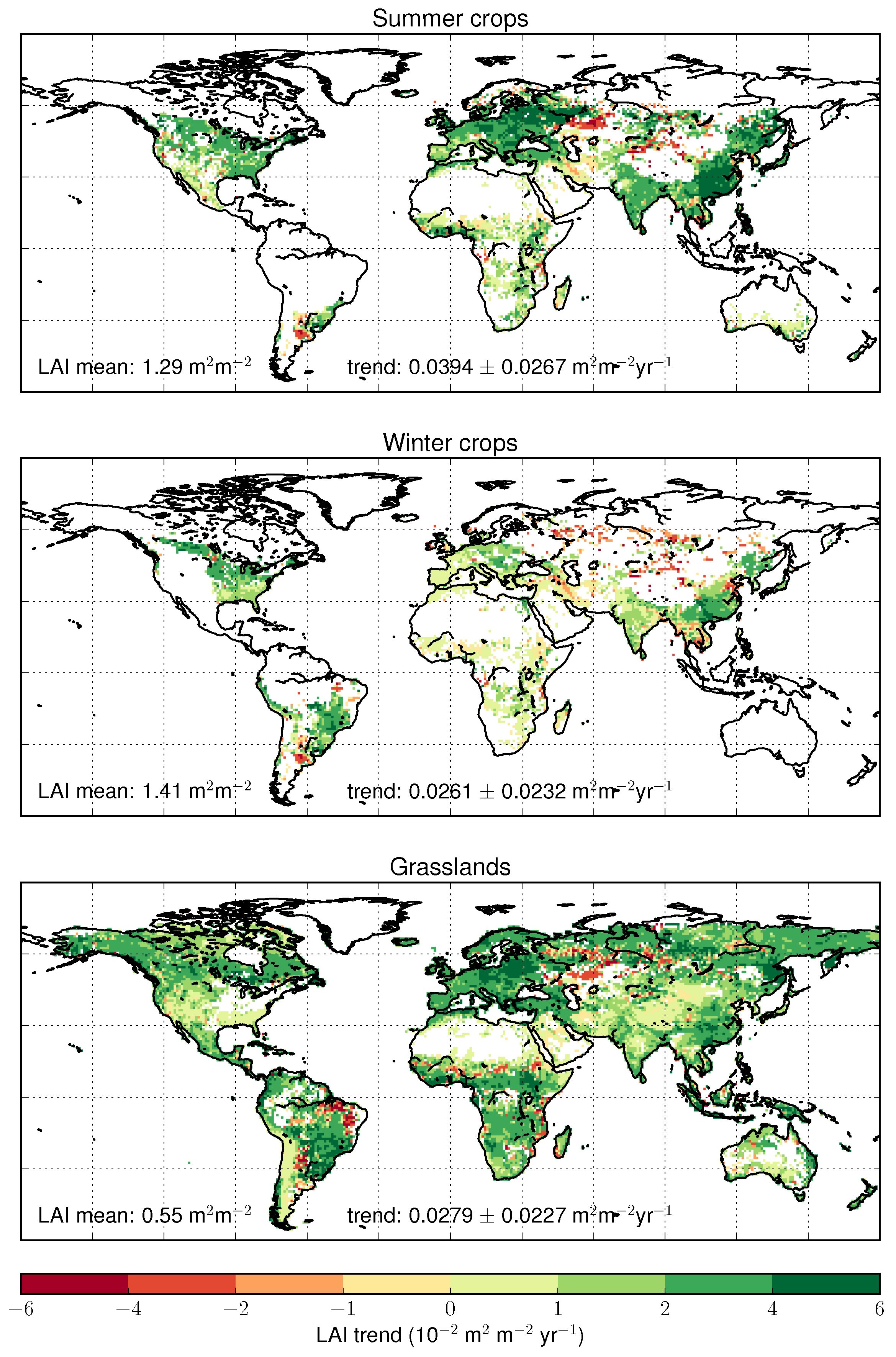
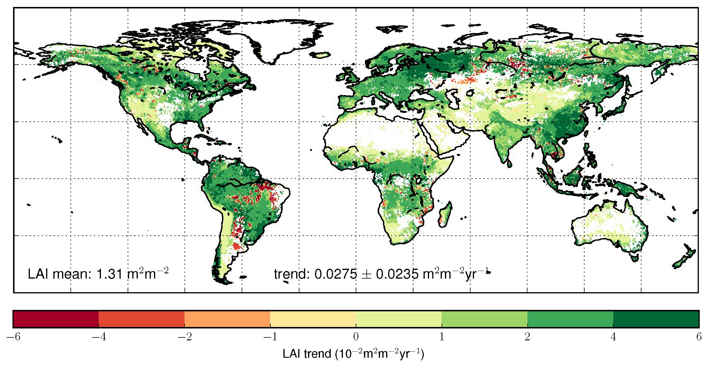
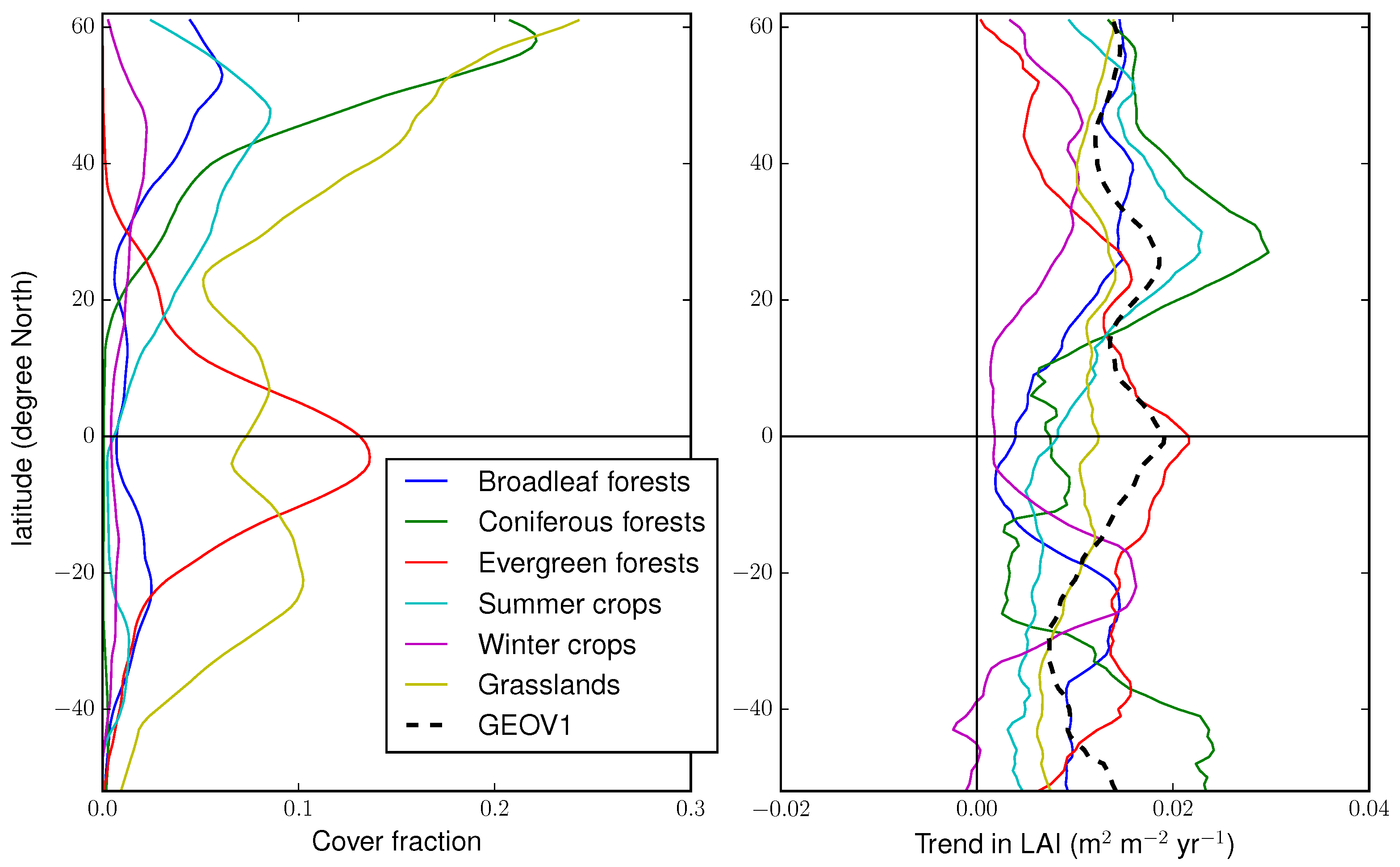
4.3. Trends Per Vegetation Types

The LAI-MC product was used to compute trends in LAI for all vegetation types all over the globe. The LAI trends of the six main vegetation types are shown in Figure 7 and Figure 8. For each vegetation type, the mean trend and its spatial standard deviation are given in Figure 7 and Figure 8. For comparison purposes, the LAI trends from the GEOV1 product was also computed (Figure 9).
Note that trend maps were spatially resampled to plot the figures, which may lead to visual overestimations of the total area with statistically significant trends (with p-values less than 0.01).
Each vegetation type shows significant positive global trends (greening) but also large spatial variabilities with standard deviations of the same order of magnitude as trends. The highest global trend is found for coniferous forests (0.0419 m 2 m 2 yr 1 ) followed by summer crops (0.0394 m 2 m 2 yr 1 ), while winter crops and grasslands show the smallest global trends (0.0261 m 2 m 2 yr 1 and 0.0279 m 2 m 2 yr 1 , respectively). For the GEOV1 total LAI, the spatial average of the statistically significant trend (p-value lower than 0.01) equals 0.0275 m 2 m 2 yr 1 with a high spatial variability (standard deviation of 0.0235 m 2 m 2 yr 1 ).
The trend maps from Figure 7 and Figure 8 are globally consistent with the trend map of the total LAI (Figure 9), especially over pixels where the cover fraction of the dominant vegetation type is close to one. Nevertheless, some differences can be reported in some regions, like in Asia or in Africa. It was shown in Figure 4 that the KF algorithm can have an significant impact on the LAI seasonal cycle. The differences between the maps in Figure 7, Figure 8 and Figure 9 show that the KF also impacts the trends. If the partitioning of LAI among the vegetation types were constant over time, trends of each vegetation type would equal trends of the total LAI from GEOV1. Figure 10 represents the standard deviation of the trends across the vegetation types (it equals 0 for pixels with only one vegetation type). The figure shows that the trend may vary significantly among vegetation types over mixed pixels. For instance, in the North-East of Europe, coniferous and broadleaf forests experience a marked greening while crops and grasslands show a significant browning. In central Asia, coniferous forests and grasslands are mainly greening whereas broadleaf forests and winter crops are browning. In the North-East of Asia, coniferous forests are browning whereas grasslands are greening. In Africa and in Europe, all vegetation types are greening but at different rates.
For each vegetation type, the average trend in LAI was compared to the trend obtained by using the single-dominant selection method. Very small differences were observed for evergreen and coniferous forests (lower than 5%). On the contrary, the relative difference is significant for other types, reaching 27% for winter crops, −39% for summer crops, 53% for broadleaf forests and −48% for grasslands. This result highlights the limited representativeness of the total LAI observed from satellite with respect to the dominant vegetation type.
The probability density function of trends for each vegetation type and for the total LAI from GEOV1 is presented in Figure 11 (no filter is applied on the p-value for this figure). Three types of behaviours can be depicted. First, broadleaf forests, grasslands and winter crops show relatively small positive trends which are quite uniform over the globe. Summer crops and coniferous show a higher spread, mostly in the positive side. Finally, evergreen forests are globally greening but at various rates ranging from 0 to 0.06 m 2 m 2 yr 1 .
Table 2 provides, for each vegetation type, the total area showing trend values larger than different thresholds. In terms of relative area, coniferous forests is the most affected by large positive trends (14% of the total coniferous forests area has trend values higher than 0.04 m 2 m 2 yr 1 ), followed by evergreen forests (11%). For very large trend values (larger than 0.06 m 2 m 2 yr 1 ), coniferous forests are still the most affected, but summer crops and broadleaf forests are more affected than evergreen forests. Regarding the absolute area, the total area covered by grasslands largely exceeds the total area of other vegetation types. The grassland area affected by very large trend values (550,000 km 2 ) is greater than for any other vegetation type, except for coniferous forests which show the largest area (720,000 km 2 ).
Table 2 also shows that the area affected by high and very high trend values (higher than 0.04 m 2 m 2 yr 1 ) is larger with LAI-MC than with GEOV1. This demonstrates the ability of LAI-MC to extract highest trend values over the different vegetation types. The “LAI-MC total” line represents the sum of all the above lines. In other terms, it accounts for areas over which any vegetation type shows trend values higher than specific thresholds. If, within a pixel equally covered by two biomes, one biome shows a very large trend value (> 0.06 m 2 m 2 yr 1 ) while the other shows a very small or negative trend value (< 0.01 m 2 m 2 yr 1 ), all the columns of the total area of LAI-MC would account for half area of this pixel. On the other hand, the LAI from GEOV1, which aggregates LAIs from both biomes, would show a medium trend value and the area of the whole pixel would be accounted for in the total area of GEOV1 LAI with medium trend values (first two columns) but not in the total area of GEOV1 LAI with very large trend values (last two columns). This explains why the total area of LAI-MC is smaller than the total area of GEOV1 for small thresholds (0.01 and 0.02 m 2 m 2 yr 1 ) and the opposite for large thresholds (0.04 and 0.06 m 2 m 2 yr 1 ). Besides, since statistically insignificant trends (p-value > 0.01) are masked out, the total area where LAI is affected by statistically significant trends (whatever the trend values) may differ between LAI-MC and GEOV1.

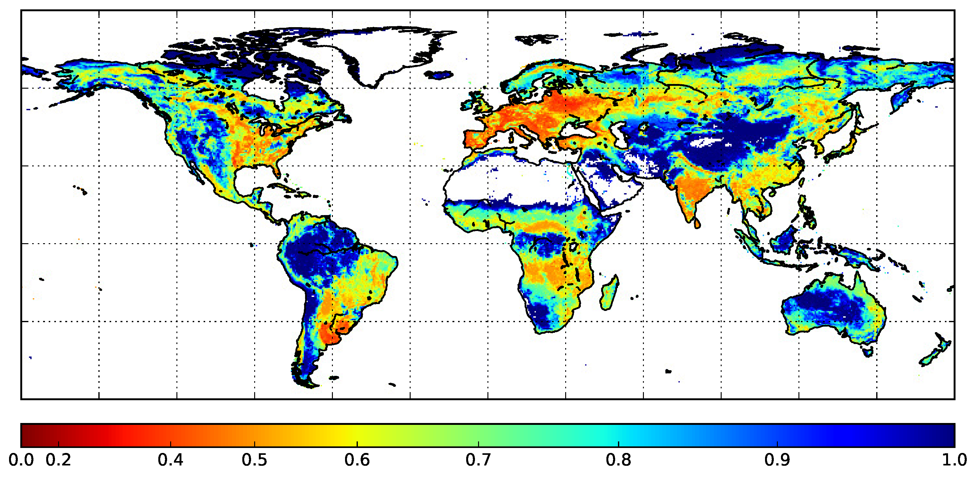
4.4. Regional Trends

As shown in Figure 7, Figure 8 and Figure 9 there is a large variability in the greening/browning all over the globe and across vegetation types.
Figure 12 presents the zonal trend (latitudinal average) for all vegetation types. The greening of grasslands only slightly depends on the latitude. For evergreen forests, the greening is larger in tropical regions where they are mostly concentrated. Other vegetation types (except for grasslands) have reduced positive trends within these regions. Coniferous and broadleaf forests are mainly greening at Northern and Southern mid-latitudes, with a higher dependency on latitude for coniferous forests. Summer crops show large positive trend values at Northern mid-latitudes and small trend values (still positive) in the Southern Hemisphere. Winter crops also show significant positive trends at Northern mid-latitudes, almost no trend near the equator and Southern high latitudes, but significant positive trends at Southern mid-latitudes. These large trend values correspond to a significant greening of winter crops in the Parana Basin (Figure 8).
Continental trends are reported in Table 3 for the GEOV1 total LAI and for the six main vegetation types. The total LAI (GEOV1) is greening quite uniformly at the continental scale, apart from Europe where greening is about 25% more intense. Except for winter crops and evergreen forests, all vegetation types experience intense greening over Europe. The greening of winter crops mostly occurs in North and South America and is quite low elsewhere. Coniferous forests show high positive trends in the three continents of the Northern Hemisphere, despite some negative values in several regions of central and Northern Asia (Figure 7). Similarly, the greening of evergreen forests is quite high and uniform over the continents of the Southern Hemisphere. Grasslands are also greening quite uniformly over the six continents, with highest values in Europe. Broadleaf forests show the most contrasted greening with small positive trends in Africa and Oceania and high positive trends in Europe and South America.
For each vegetation type, LAI trends have also been averaged over four main climate zones established from the Köppen-Geiger classification map [62]: boreal, temperate, arid and tropical (Figure 13). Trends are reported in Table 4. For each climate region, the greening of the different vegetation types is quite uniform, with some exception corresponding to very small cover areas such as evergreen forests in boreal climate areas. The climate zones that experience the highest greening are boreal and temperate regions, followed by tropical regions. Arid climate regions show quite small trend values, but still positive. Temperate and boreal climates show the two largest greening trends, especially for forests and summer crops. Summer crops are also greening at a quite high rate in arid and tropical regions. In arid regions, the greening is quite small for all types of vegetation. The highest value is for summer crops, which could be related to anthropogenic effects such as irrigation.

5. Discussion

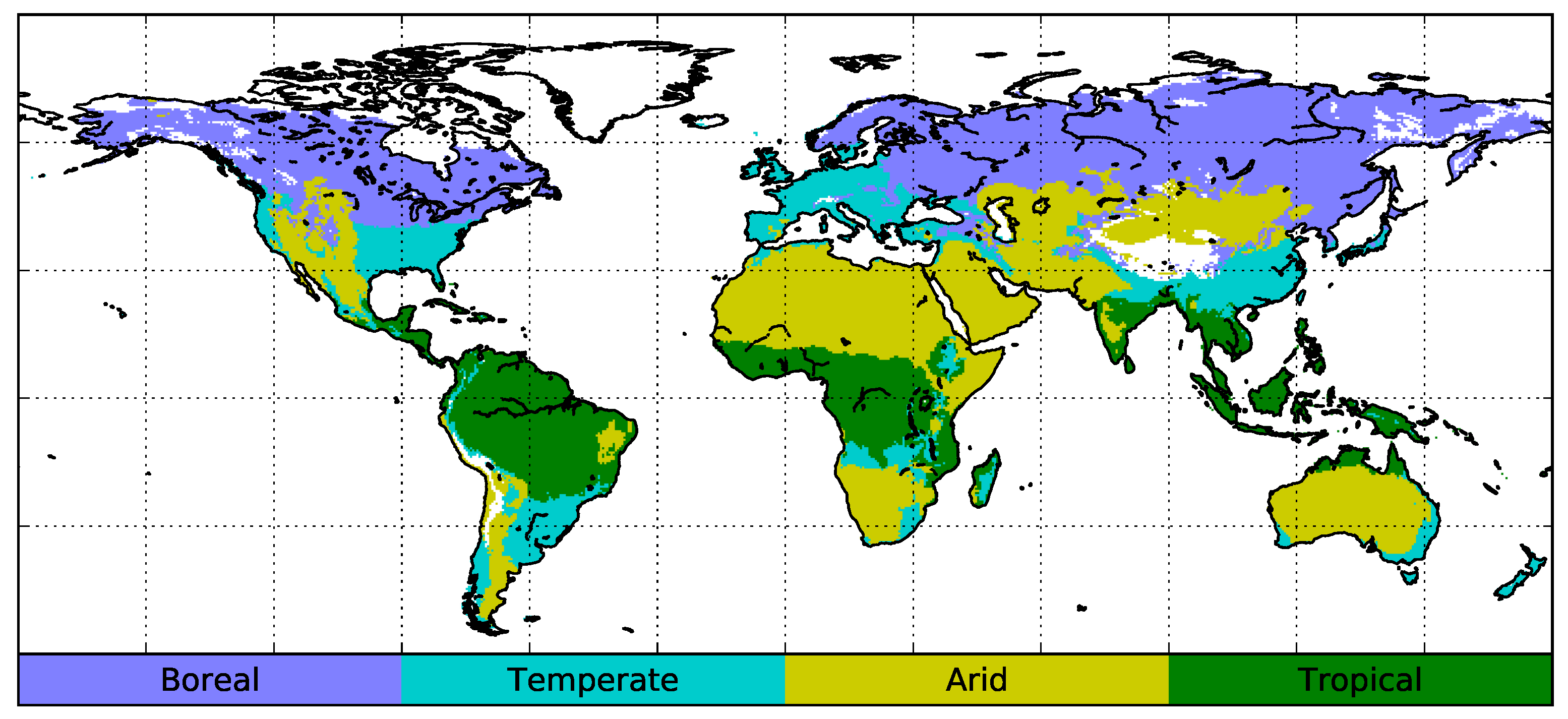
5.1. Relationship Between Vegetation Dynamics and Climate

Several studies can be found in the literature on the causes of vegetation greening or browning over different regions of the globe. For instance, Forzieri, G. and Alkama, R. et al. [18] focused on the interplay between LAI and the terms of the energy balance. They showed that in cold-temperate and boreal regions, LAI increased with absorbed radiation. By contrast, in warm regions, the increase in LAI is associated with cooling and an enhancement of the latent heat flux. Radiative terms of the energy budget then dominate the relationship with LAI in cold regions, while it is dominated by turbulent energy fluxes in warm regions.
Feng, H. et al. [22] showed that the vegetation dynamics is highly correlated to precipitation mainly at middle latitudes of the Southern Hemisphere, where our results depict a marked greening mostly for winter crops, broadleaf and evergreen forests. On the contrary, precipitation and vegetation growth are mainly anti-correlated at high latitudes of the Northern Hemisphere [22], where summer crops, grasslands and broadleaf and coniferous forests show large positive trends ranging from 0.01 m 2 m 2 yr 1 to 0.03 m 2 m 2 yr 1 (see, e.g., Figure 12).
In the tropical zone, evergreen forests and grasslands are rapidly greening (see Table 4), which seems to be related to rising CO 2 in the atmosphere [14]. On the contrary, in high latitudes of the Northern Hemisphere where coniferous forests are dominating, Zhu, Z. et al. [14] suggested that changes in the vegetation dynamics are mainly driven by climate change. Although spatial patterns of the GEOV1 total LAI match well those obtained by Zhu, Z. et al. [14], they found a global greening trend of 0.068 m 2 m 2 yr 1 , which is significantly greater than for GEOV1 (0.028 m 2 m 2 yr 1 ). The difference may be explained by two main factors: (1) Zhu, Z. et al. [14] used three different satellite datasets (GIMMS LAI3g [63], GLOBMAP [64] and GLASS [65]) over a different time period (1982–2009 while 1999–2015 was considered in this study) and (2) they considered only the growing season to compute the trends.
Piao, S. et al. [12] reported a greening of vegetation in China, except over Northern China and Inner Mongolia where climate change has mainly a negative impact on vegetation growth, probably due to more frequent or intense droughts during the past decades. Our results show that winter crops and coniferous forests are browning in these regions. By contrast, grasslands have positive trends.
The latitudinal asymmetry of trends (i.e., larger trend values in the Northern hemisphere) as depicted by several authors (see e.g., [11]) is also clearly shown in our results (see Figure 12). This asymmetry is mainly attributed to the south-to-north asymmetric land surface warming and CO 2 fertilization [11]. In the LAI-MC product, this phenomenon is clearly visible for summer crops, broadleaf forests and grasslands. It is less obvious for coniferous forests and winter crops which show high positive peaks at both Northern and Southern mid-latitudes and it seems even inverted for evergreen forests.

5.2. Northern Mid and High Latitudes

Vegetation greening in the Northern mid-latitudes was reported in several studies. Zhu, Z. et al. [66] used ten ecosystem models and suggested that the positive trends during summer, autumn and spring in the Northern latitudes ( > 30 N) are mainly due to elevating atmospheric CO 2 concentration. The effects of nitrogen deposition and land use change would be relatively small. Wu, X. et al. [32] studied the interannual temperature sensitivity of mean growing season NDVI for forest, shrub and grassland PFTs over Northern Hemisphere and found that for all vegetation types the sensitivity decreases with higher interannual variability in temperature. According to Wu, X. et al. [32], the decrease is larger in taller forest and shrub in water-limited arid and temperate climate zones. By using the SURFEX modeling plateform, Laanaia, N. et al. [67] also found that air temperature is the main driver of changes in leaf onset dates for crops, grasslands and forests over France. By contrast, leaf senescence dates were found to be more sensitive to changes in soil moisture stress periods.
Our results are consistent with overall greening in Northern latitudes, but some vegetation types seem to be browning, especially in central Asia (winter crops, broadleaf forests). The decreasing LAI trends of taller plants in water-limited regions are likely due to increased mortality during the past decades [68].
Other studies reported vegetation greening in the Arctic regions [69,70]. Our LAI-MC product shows increasing trends for grasslands but decreasing trends for coniferous forests. This result is in agreement with Beck, P.S. and Goetz, S.J. [71] who reported a decreasing productivity over dense forests, along an evergreen-deciduous gradient or a shrub cover gradient. Beck, P.S. and Goetz, S.J. [71] attributed the browning in Northeastern America and Eurasia mostly to forest disturbances, namely to a succession of fires during the last decades. In addition, by using an ensemble of Earth System Models with dynamic vegetation and anthropogenic factors, Mao, J. et al. [72] showed evidences of human fingerprint on vegetation dynamics in the Northern mid and high latitudes.

5.3. Arid and Semi-Arid Areas

Fensholt, R. et al. [73] studied trends in vegetation dynamics in semi-arid regions all over the globe. They reported an increase in greenness in semi-arid areas where plant growth is mainly limited by precipitation or constrained by air temperature. Our results also indicate positive trends essentially for grasslands in these areas, namely in the Northern India, Turkey and Northern USA.
In arid and semi-arid regions of the Southern hemisphere, Forzieri, G. et al. [18] related trends in LAI to regional cooling trends due to the close link between vegetation cover and latent heat flux in water-limited regions. In the Sahel, slightly positive trends (for grasslands and crops as shown in Figure 7 and Figure 8) may be partly explained by the recent increase in precipitation and by land use management [74].
In the semi-arid region of Inner Asia, decreasing precipitation and increasing atmospheric water demand were responsible for a decline of tree growth over the last two decades, as shown by records of tree-ring widths [24]. This results is in agreement with Figure 7 that shows negative trends of coniferous forests in this region.

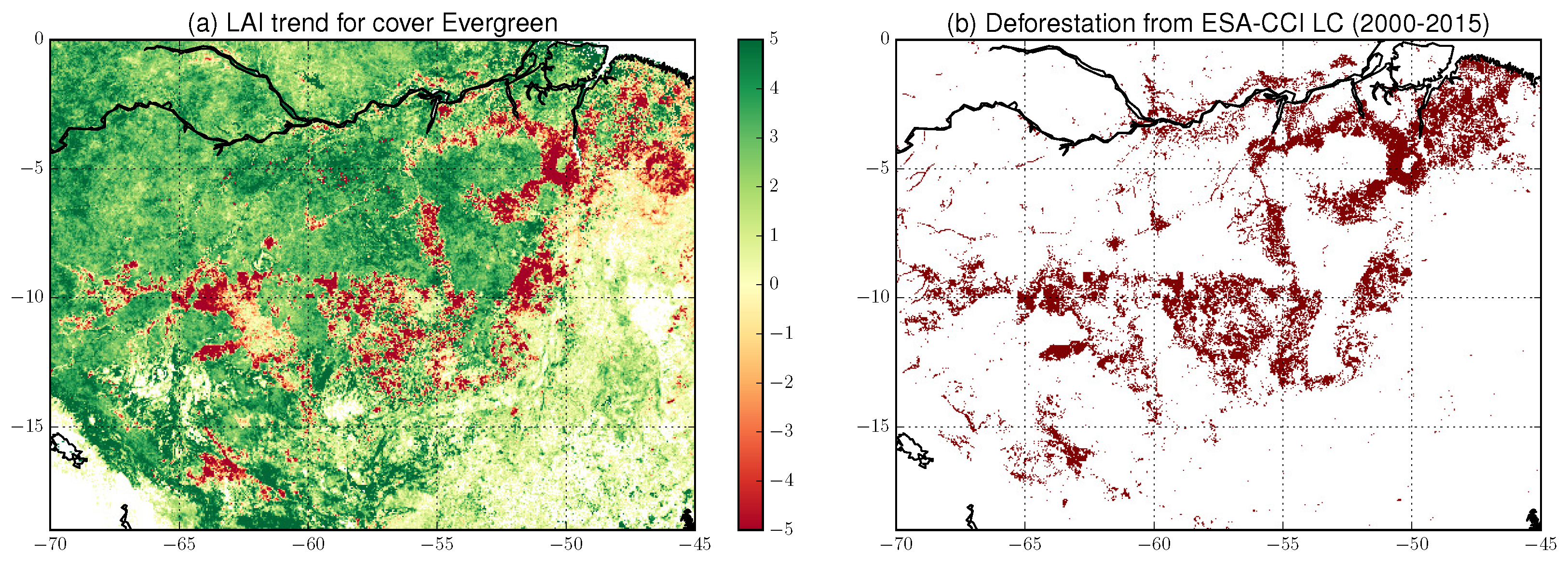
5.4. Forests and Land Cover Change

Land Cover change significantly affects the water, energy and carbon cycles [75]. More than half of the global land surfaces are covered by natural vegetation, which changed significantly in the past decades, particularly over regions covered by forests [76,77]. Vegetation changes due to human activities may have altered more than 40% of terrestrial surfaces, potentially reducing the global terrestrial evapotranspiration by up to 5% [75].
A very dense literature can be found on forest changes and their relation with climate. In particular, deforestation rates have been increasing in the tropics and decreasing in other regions. These changes in forest cover are mainly due to anthropogenic practices [76] and to natural factors such as forest fires and extreme climate conditions [78,79].
Changes in global and local forest cover significantly impacts the climate, with cooling or warming effects depending on the region [80]. For instance, Lee, X. et al. [81] reported that deforestation could lead to cooling effects in the Northern high latitudes and reversely to warming effects below 35 N. The positive/negative trend patterns from our study are largely consistent with the reported warming effects of Northern afforestation and reforestation [18,80,81]. For instance, the large greening trends of forests in China may be partly explained by human activities such as afforestation and agricultural management [25].
The derivation of the LAI-MC product relies on the ECOCLIMAP-II land cover database which provides the cover fraction of each vegetation type for each pixel. This database is static and then does not represent land cover changes. In case of deforestation, the mean LAI values are likely to decrease. This is particularly true for evergreen forests. For example, browning is observed in the Southern part of the Amazon Basin (see Figure 14a). We used ESA-CCI Land Cover maps [29] for the years 2000 and 2015 to detect pixels that were covered by forest in 2000 and not in 2015 (Figure 14b). There is a clear match between patterns of highly negative trends from LAI-MC (evergreen forests) and deforestated areas from ESA-CCI LC. Pixels affected by deforestation in the Amazon basin are largely dominated by evergreen forests, which explains that similar patterns of negative trends can be found in the GEOV1 trend map (Figure 9). Figure 14a demonstrates that the disaggregation process does not prevent LAI-MC from detecting deforestation (large negative trends). Deeper analyses could be performed by studying breaks in the LAI signal, as done by Planque, C. et al. [34] using the Zeileis’ method [82]. Such a study could help diagnosing land cover changes for forests as well as for other vegetation types.
To get a better idea of the impact of land cover change on the resulting LAI-MC trends, we used both 2000 and 2015 ESA-CCI Land Cover maps to detect pixels affected by land cover change. It resulted that about 2.7% of the global vegetated area have faced land cover change between 2000 and 2015 (2.7% for forests, 2.9% for crops and 2.5% for grasslands). To quantify the impact on LAI-MC trends, the land cover change map was used to mask out the affected pixels. When comparing new trend values with Table 3, it appears that land cover change has a small impact on the results. Trends of evergreen forests are the most affected by land cover change (4% greater in South America). The impact on other vegetation types is smaller than 2%. Although further developments could include land cover change within the disaggregation method, we conclude that the disaggregation method, which relies on a static land cover map, is a reliable first order approximation.

6. Conclusions

This study presents an innovative method to disaggregate the total LAI observed from satellites into LAIs of several vegetation types, including broadleaf, evergreen and coniferous forests, grasslands and summer/winter crops. The algorithm is an extension of the method from Carrer, D. et al. [33] to reconstruct bare soil and vegetation albedos from total albedo. It is based on a Kalman Filter approach and makes use of cover fraction and LAI seasonal cycle per vegetation types from the ECOCLIMAP-II database as prior information. The derived product, called LAI-MC (Multi-Cover), consists of world-wide LAI maps provided every 10 days for each vegetation type over the period 1999–2015. The LAI-MC product is validated against in situ measurements with overall good performances, at least as good as for the total LAI, even for pixels where the vegetation type corresponding to the local site is not dominant.
A trend analysis is performed at the global scale and over different regions (continents and climate zones). On average, all vegetation types have experienced greening over the last two decades at rates ranging from 0.026 m 2 m 2 yr 1 for winter crops to 0.042 m 2 m 2 yr 1 for coniferous forests. Coniferous forests are mainly greening in temperate regions and show the largest area affected by high positive trends. By contrast, grasslands are greening at a moderate average rate, but since they cover almost half of the total vegetated area, the grassland area affected by high trend values is greater than for any other vegetation type but coniferous forests. Evergreen forests, which are mainly located in the tropical regions, show high positive trends except for deforested areas of the Amazon Basin. Coniferous and broadleaf forests have been browning in Central Asia and greening in most other regions of the Northern Hemisphere. Globally, grasslands and summer crops experienced greening while winter crops show small or even negative trends.
These results are in agreement with previous studies on the regions of the world that show greening or browning. Nevertheless, some differences can be noted among vegetation types that other studies could not identify. For instance, our study shows that coniferous forests of Central Asia are greening while broadleaf forests in the same region are mostly browning. In the North-Eastern part of Asia, coniferous and broadleaf forests are greening while grasslands are browning. Coniferous forests, winter and summer crops and grassland in China are all greening but at different rates. The same remark applies for South America.
LAI trends of each vegetation type are compared to the single-dominant selection method (obtained by considering only the dominant vegetation type for each pixel). Small differences are observed for evergreen and coniferous forests. On the contrary, the spatial average of the relative difference reaches ±27% to 53% for other vegetation types. This result highlights the limited representativeness of the total LAI with respect to the dominant vegetation type, as well as the added value of the LAI-MC disaggregated product.
Finally, the new LAI-MC dataset is the first product providing global maps of vegetation growth every 10 days for the main vegetation types over the last 17 years. Although the problem of detection/attribution is behind the scope of this study, the LAI-MC product can help such analyses by offering a more consistent comparison with observations and derived products. Apart from climate related studies, it may be valuable for Land Surface Models (LSMs) to update phenology parameters. Also the assimilation of satellite derived LAI observations into the ISBA LSM as done recently by Albergel, C. and Munier, S. et al. [83] is based on the comparison between the total observed LAI and the aggregated LAI simulated over the different vegetation types. An extension is under development to assimilate the disaggregated LAI-MC product for each vegetation type independently, with very promising preliminary results.

Supplementary Materials

Supplementary Materials: The following are available online at https://www.mdpi.com/2072-4292/10/3/424/s1.

Acknowledgments

The work of Simon Munier was supported by European Union Seventh Framework Programme (FP7/2007-2013) under grant agreement No. 603608, “Global Earth Observation for integrated water resource assessment” (eartH2Observe). The work of Carole Planque was suppoted by Météo France and Région Midi-Pyrénées. The authors acknowledge the Copernicus Global Land service for providing the satellite-derived LAI products. The authors would like to thank Stéphanie Faroux and Catherine Meurey for initial discussions in the scope of ECOCLIMAP-SG, as well as the anonymous reviewers for their insightful comments.

Author Contributions

S.M. and D.C. conceived and designed the experiments; S.M. and C.P. performed the experiments; F.C. provided in situ LAI measurements; S.M., D.C., C.A. and J.-C.C. analyzed the results; S.M. wrote the paper.

Conflicts of Interest

The authors declare no conflict of interest.

References

  1. Sellers, P.J.; Dickinson, R.E.; Randall, D.A.; Betts, A.K.; Hall, F.G.; Berry, J.A.; Collatz, G.J.; Denning, A.S.; Mooney, H.A.; Nobre, C.A.; et al. Modeling the exchange of energy, water, and carbon between continents and atmosphere. Science 1997, 275, 502–509. [Google Scholar] [CrossRef] [PubMed]
  2. Chen, J.M.; Black, T.A. Defining leaf area index for non-flat leaves. Plant Cell Environ. 1992, 15, 421–429. [Google Scholar] [CrossRef]
  3. GCOS. Systematic Observation Requirements for Satellite-Based Products for Climate: 2011 Update; GCOS-154; World Meteorological Organization: Geneva, Switzerland, 2011. [Google Scholar]
  4. Turner, D.P.; Cohen, W.B.; Kennedy, R.E.; Fassnacht, K.S.; Briggs, J.M. Relationships between leaf area index, FAPAR and net primary production of terrestrial ecosystems. Remote Sens. Environ. 1999, 70, 52–68. [Google Scholar] [CrossRef]
  5. Zhang, P.; Anderson, B.; Tan, B.; Huang, D.; Myneni, R. Potential monitoring of crop production using a satellite-based Climate-Variability Impact Index. Agric. For. Meteorol. 2005, 132, 344–358. [Google Scholar] [CrossRef]
  6. Buermann, W.; Dong, J.; Zeng, X.; Myneni, R.B.; Dickinson, R.E. Evaluation of the utility of satellite-based vegetation leaf area index data for climate simulations. J. Clim. 2001, 14, 3536–3550. [Google Scholar] [CrossRef]
  7. Chase, T.N.; Pielke, R.A.; Kittel, T.G.; Nemani, R.; Running, S.W. Sensitivity of a general circulation model to global changes in leaf area index. J. Geophys. Res. D Atmos. 1996, 101, 7393–7408. [Google Scholar] [CrossRef]
  8. Nunes, C.; Auge, J.I. Land-Use and Land-Cover Change (LUCC): Implementation Strategy; IGBP Report-48; University of North Texas Libraries, Digital Librar: Stockholm, Sweden, 1999. [Google Scholar]
  9. Fang, H.; Jiang, C.; Li, W.; Wei, S.; Baret, F.; Chen, J.M.; Garcia-Haro, J.; Liang, S.; Liu, R.; Myneni, R.B.; et al. Characterization and intercomparison of global moderate resolution leaf area index (LAI) products: Analysis of climatologies and theoretical uncertainties. J. Geophys. Res. Biogeosci. 2013, 118, 529–548. [Google Scholar] [CrossRef]
  10. Los, S.O. Analysis of trends in fused AVHRR and MODIS NDVI data for 1982–2006: Indication for a CO2 fertilization effect in global vegetation. Glob. Biogeochem. Cycles 2013, 27, 318–330. [Google Scholar] [CrossRef]
  11. Mao, J.; Shi, X.; Thornton, P.E.; Hoffman, F.M.; Zhu, Z.; Myneni, R.B. Global latitudinal-asymmetric vegetation growth trends and their driving mechanisms: 1982–2009. Remote Sens. 2013, 5, 1484–1497. [Google Scholar] [CrossRef]
  12. Piao, S.; Yin, G.; Tan, J.; Cheng, L.; Huang, M.; Li, Y.; Liu, R.; Mao, J.; Myneni, R.B.; Peng, S.; et al. Detection and attribution of vegetation greening trend in China over the last 30 years. Glob. Chang. Biol. 2015, 21, 1601–1609. [Google Scholar] [CrossRef] [PubMed]
  13. Xu, L.; Myneni, R.B.; Chapin, F.S., III; Callaghan, T.V.; Pinzon, J.E.; Tucker, C.J.; Zhu, Z.; Bi, J.; Ciais, P.; Tømmervik, H.; et al. Temperature and vegetation seasonality diminishment over northern lands. Nat. Clim. Chang. 2013, 3, 581–586. [Google Scholar] [CrossRef] [Green Version]
  14. Zhu, Z.; Piao, S.; Myneni, R.B.; Huang, M.; Zeng, Z.; Canadell, J.G.; Ciais, P.; Sitch, S.; Friedlingstein, P.; Arneth, A.; et al. Greening of the Earth and its drivers. Nat. Clim. Chang. 2016, 6, 791–795. [Google Scholar] [CrossRef]
  15. Planque, C.; Carrer, D.; Roujean, J.L. Analysis of MODIS albedo changes over steady woody covers in France during the period of 2001–2013. Remote Sens. Environ. 2017, 191, 13–29. [Google Scholar] [CrossRef]
  16. Bonan, G.B. Forests and climate change: forcings, feedbacks, and the climate benefits of forests. Science 2008, 320, 1444–1449. [Google Scholar] [CrossRef] [PubMed]
  17. Sitch, S.; Friedlingstein, P.; Gruber, N.; Jones, S.D.; Murray-Tortarolo, G.; Ahlström, A.; Doney, S.C.; Graven, H.; Heinze, C.; Huntingford, C.; et al. Recent trends and drivers of regional sources and sinks of carbon dioxide. Biogeosciences 2015, 12, 653–679. [Google Scholar] [CrossRef] [Green Version]
  18. Forzieri, G.; Alkama, R.; Miralles, D.G.; Cescatti, A. Satellites reveal contrasting responses of regional climate to the widespread greening of Earth. Science 2017, 356, 1180–1184. [Google Scholar] [CrossRef] [PubMed]
  19. Anderson, R.G.; Canadell, J.G.; Randerson, J.T.; Jackson, R.B.; Hungate, B.A.; Baldocchi, D.D.; Ban-Weiss, G.A.; Bonan, G.B.; Caldeira, K.; Cao, L.; et al. Biophysical considerations in forestry for climate protection. Front. Ecol. Environ. 2011, 9, 174–182. [Google Scholar] [CrossRef]
  20. Chapin, F.S.; Randerson, J.T.; McGuire, A.D.; Foley, J.A.; Field, C.B. Changing feedbacks in the climate–biosphere system. Front. Ecol. Environ. 2008, 6, 313–320. [Google Scholar] [CrossRef]
  21. Bright, R.M.; Davin, E.; O’Halloran, T.; Pongratz, J.; Zhao, K.; Cescatti, A. Local temperature response to land cover and management change driven by non-radiative processes. Nat. Clim. Chang. 2017, 7, 296–302. [Google Scholar] [CrossRef]
  22. Feng, H.; Zou, B.; Luo, J. Coverage-dependent amplifiers of vegetation change on global water cycle dynamics. J. Hydrol. 2017, 550, 220–229. [Google Scholar] [CrossRef]
  23. Calvet, J.C. Investigating soil and atmospheric plant water stress using physiological and micrometeorological data. Agric. For. Meteorol. 2000, 103, 229–247. [Google Scholar] [CrossRef]
  24. Liu, H.; Park Williams, A.; Allen, C.D.; Guo, D.; Wu, X.; Anenkhonov, O.A.; Liang, E.; Sandanov, D.V.; Yin, Y.; Qi, Z.; et al. Rapid warming accelerates tree growth decline in semi-arid forests of Inner Asia. Glob. Chang. Biol. 2013, 19, 2500–2510. [Google Scholar] [CrossRef] [PubMed]
  25. Pan, Y.; Birdsey, R.A.; Fang, J.; Houghton, R.; Kauppi, P.E.; Kurz, W.A.; Phillips, O.L.; Shvidenko, A.; Lewis, S.L.; Canadell, J.G.; et al. A large and persistent carbon sink in the world’s forests. Science 2011, 333, 988–993. [Google Scholar] [CrossRef] [PubMed]
  26. Liang, E.; Eckstein, D.; Liu, H. Assessing the recent grassland greening trend in a long-term context based on tree-ring analysis: A case study in North China. Ecol. Indic. 2009, 9, 1280–1283. [Google Scholar] [CrossRef]
  27. Chen, B.; Zhang, X.; Tao, J.; Wu, J.; Wang, J.; Shi, P.; Zhang, Y.; Yua, C. The impact of climate change and anthropogenic activities on alpine grassland over the Qinghai-Tibet Plateau. Agric. For. Meteorol. 2014, 189, 11–18. [Google Scholar] [CrossRef]
  28. Carlyle, C.N.; Fraser, L.H.; Turkington, R. Response of grassland biomass production to simulated climate change and clipping along an elevation gradient. Oecologia 2014, 174, 1065–1073. [Google Scholar] [CrossRef] [PubMed]
  29. Bontemps, S.; Defourny, P.; Radoux, J.; Van Bogaert, E.; Lamarche, C.; Achard, F.; Mayaux, P.; Boettcher, M.; Brockmann, C.; Kirches, G.; et al. Consistent global land cover maps for climate modelling communities: Current achievements of the ESA’s land cover CCI. In Proceedings of the ESA Living Planet Symposium, Edimburgh, UK, 9–13 September 2013; pp. 9–13. [Google Scholar]
  30. Faroux, S.; Kaptué Tchuenté, A.T.; Roujean, J.L.; Masson, V.; Martin, E.; Le Moigne, P. ECOCLIMAP-II/Europe: A twofold database of ecosystems and surface parameters at 1 km resolution based on satellite information for use in land surface, meteorological and climate models. Geosci. Model Dev. 2013, 6, 563–582. [Google Scholar] [CrossRef]
  31. Baret, F.; Weiss, M.; Lacaze, R.; Camacho, F.; Makhmara, H.; Pacholcyzk, P.; Smets, B. GEOV1: LAI and FAPAR essential climate variables and FCOVER global time series capitalizing over existing products. Part1: Principles of development and production. Remote Sens. Environ. 2013, 137, 299–309. [Google Scholar] [CrossRef]
  32. Wu, X.; Liu, H.; Li, X.; Piao, S.; Ciais, P.; Guo, W.; Yin, Y.; Poulter, B.; Peng, C.; Viovy, N.; et al. Higher temperature variability reduces temperature sensitivity of vegetation growth in Northern Hemisphere. Geophys. Res. Lett. 2017, 44, 6173–6181. [Google Scholar] [CrossRef]
  33. Carrer, D.; Meurey, C.; Ceamanos, X.; Roujean, J.L.; Calvet, J.C.; Liu, S. Dynamic mapping of snow-free vegetation and bare soil albedos at global 1km scale from 10-year analysis of MODIS satellite products. Remote Sens. Environ. 2014, 140, 420–432. [Google Scholar] [CrossRef]
  34. Planque, C.; Carrer, D.; Leroux, D.J.; Pinault, F.; Roujean, J.-L.; Munier, S. Analyzing the albedo evolutions over pure forest land cover in France during the 2001–2013 period. In Proceedings of the MultiTemp 2017, Bruges, Belgium, 27–29 June 2017. [Google Scholar]
  35. Verrelst, J.; Camps-Valls, G.; Muñoz-Marí, J.; Rivera, J.P.; Veroustraete, F.; Clevers, J.G.; Moreno, J. Optical remote sensing and the retrieval of terrestrial vegetation bio-geophysical properties—A review. ISPRS J. Photogramm. Remote Sens. 2015, 108, 273–290. [Google Scholar] [CrossRef]
  36. Myneni, R.B.; Hoffman, S.; Knyazikhin, Y.; Privette, J.L.; Glassy, J.; Tian, Y.; Wang, Y.; Song, X.; Zhang, Y.; Smith, G.R.; et al. Global products of vegetation leaf area and fraction absorbed PAR from year one of MODIS data. Remote Sens. Environ. 2002, 83, 214–231. [Google Scholar] [CrossRef]
  37. Baret, F.; Hagolle, O.; Geiger, B.; Bicheron, P.; Miras, B.; Huc, M.; Berthelot, B.; Niño, F.; Weiss, M.; Samain, O.; et al. LAI, fAPAR and fCover CYCLOPES global products derived from VEGETATION: Part 1: Principles of the algorithm. Remote Sens. Environ. 2007, 110, 275–286. [Google Scholar] [CrossRef] [Green Version]
  38. Smets, B.; Lacaze, R. Gio Global Land Component—Lot I “Operation of the Global Land Component”—Product User Manual. 2013. Available online: https://land.copernicus.eu/global/sites/cgls.vito.be/files/products/GIOGL1_PUM_LAIV1_I1.10.pdf (accessed on 20 February 2018).
  39. Camacho, F.; Cernicharo, J.; Lacaze, R.; Baret, F.; Weiss, M. GEOV1: LAI, FAPAR essential climate variables and FCOVER global time series capitalizing over existing products. Part 2: Validation and intercomparison with reference products. Remote Sens. Environ. 2013, 137, 310–329. [Google Scholar] [CrossRef]
  40. Camacho, F.; Sánchez, J.; Sánchez-Azofeif, A.; Calvo-Rodríguez, S. GIO Global Land Component—Lot I “Operation of the Global Land Component”, Framework Service Contract No 388533 (JRC), Quality Assessment Report, PROBA-V GEOV1 LAI, FAPAR, FCover; EC Copernicus Global Land: Brussels, Belgium, 2017. [Google Scholar]
  41. Weiss, M.; Baret, F.; Block, T.; Koetz, B.; Burini, A.; Scholze, B.; Lecharpentier, P.; Brockmann, C.; Fernandes, R.; Plummer, S.; et al. On Line Validation Exercise (OLIVE): A web based service for the validation of medium resolution land products. Application to FAPAR products. Remote Sens. 2014, 6, 4190–4216. [Google Scholar] [CrossRef] [Green Version]
  42. Camacho, F.; Latorre, C.; Lacaze, R.; Sanchez-Zapero, J.; Baret, F.; Weiss, M. Coauthors Protocol for building a consistent database for accuracy assessment of LAI, FAPAR and FCOVER satellite products: The ImagineS database. Remote Sens. Environ. 2018. submitted. [Google Scholar]
  43. Garrigues, S.; Lacaze, R.; Baret, F.; Morisette, J.T.; Weiss, M.; Nickeson, J.E.; Fernandes, R.; Plummer, S.; Shabanov, N.V.; Myneni, R.B.; et al. Validation and intercomparison of global Leaf Area Index products derived from remote sensing data. J. Geophys. Res. Biogeosci. 2008, 113, G02028. [Google Scholar] [CrossRef]
  44. Cohen, W.B.; Maiersperger, T.K.; Turner, D.P.; Ritts, W.D.; Pflugmacher, D.; Kennedy, R.E.; Kirschbaum, A.; Running, S.W.; Costa, M.; Gower, S.T. MODIS land cover and LAI collection 4 product quality across nine sites in the western hemisphere. IEEE Trans. Geosci. Remote Sens. 2006, 44, 1843–1857. [Google Scholar] [CrossRef]
  45. Privette, J.L.; Tian, Y.; Roberts, G.; Scholes, R.J.; Wang, Y.; Caylor, K.; Mukelabai, M. Structural characterization and relationships in Kalahari woodlands and savanna. Glob. Chang. Biol. 2004, 10, 281–291. [Google Scholar] [CrossRef]
  46. Yang, W.; Huang, D.; Tan, B.; Stroeve, J.C.; Shabanov, N.V.; Knyazikhin, Y.; Nemani, R.R.; Myneni, R.B. Analysis of leaf area index and fraction of PAR absorbed by vegetation products from the Terra MODIS sensor: 2000–2005. IEEE Trans. Geosci. Remote Sens. 2006, 44, 1829–1842. [Google Scholar] [CrossRef]
  47. Abuelgasim, A.A.; Fernandes, R.A.; Leblanc, S.G. Evaluation of national a global LAI products derived from optical remote sensing instrument over Canada. IEEE Trans. Geosci. Remote Sens. 2006, 44, 1872–1884. [Google Scholar] [CrossRef]
  48. Iiames, J.S.; Pilant, A.N.; Lewis, T.E. In-situ estimates of forest LAI for MODIS data validation. In Remote Sensing and GIS Accuracy Assessment; Lunetta, R.S., Lyon, J.G., Eds.; CRC: Boca Raton, FL, USA, 2004; pp. 41–58. [Google Scholar]
  49. Chen, J.M.; Rich, P.M.; Gower, S.T.; Norman, J.M.; Plummer, S. Leaf area index of boreal forests: Theory, techniques, and measurements. J. Geophys. Res. Atmos. 1997, 102, 29429–29443. [Google Scholar] [CrossRef]
  50. Jonckheere, I.; Fleck, S.; Nackaerts, K.; Muys, B.; Coppin, P.; Weiss, M.; Baret, F. Reviews of methods for in situ leaf area index determination. Part I. Theories, sensors, and hemispherical photography. Agric. For. Meteorol. 2004, 121, 19–35. [Google Scholar] [CrossRef]
  51. Demarez, V.; Duthoit, S.; Baret, F.; Weiss, M.; Dedieu, G. Estimation of leaf area and clumping indexes of crops with hemispherical photographs. Agric. For. Meteorol. 2008, 148, 644–655. [Google Scholar] [CrossRef] [Green Version]
  52. INRA. CAN-EYE. INRA, Avignon, France, v6.47 Edition. 2016. Available online: http://www6.paca.inra.fr/can-eye (accessed on 7 March 2018).
  53. Morisette, J.T.; Baret, F.; Privette, J.L.; Myneni, R.B.; Nickeson, J.E.; Garrigues, S.; Shabanov, N.V.; Weiss, M.; Fernandes, R.; Leblanc, S.G.; et al. Validation of global moderate resolution LAI products: A framework proposed within the CEOS land product validation subgroup. IEEE Trans. Geosci. Remote Sens. 2006, 44, 1804–1817. [Google Scholar] [CrossRef]
  54. Fernandes, R.; Plummer, S.; Nightingale, J.; Baret, F.; Camacho, F.; Fang, H.; Garrigues, S.; Gobron, N.; Lang, M.; Lacaze, R.; et al. Global Leaf Area Index Product Validation Good Practices. In Best Practice for Satellite-Derived Land Product Validation; Fernandes, R., Plummer, S., Nightingale, J., Eds.; Version 2.0: Public Version Made Available on LPV Website; Land Product Validation Subgroup (WGCV/CEOS): Greenbelt, MD, USA, 2014; pp. 1–78. [Google Scholar]
  55. Cohen, W.B.; Justice, C.O. Validating MODIS terrestrial ecology products: Linking in situ and satellite measurements. Remote Sens. Environ. 1999, 70, 1–3. [Google Scholar] [CrossRef]
  56. Martìnez, B.; García-Haro, F.J.; Camacho, F. Derivation of high-resolution leaf area index maps in support of validation activities: Application to the cropland Barrax site. Agric. For. Meteorol. 2009, 149, 130–145. [Google Scholar] [CrossRef]
  57. Noilhan, J.; Mahfouf, J.-F. The ISBA land surface parameterisation scheme. Glob. Planet. Chang. 1996, 13, 145–159. [Google Scholar] [CrossRef]
  58. Masson, V.; Le Moigne, P.; Martin, E.; Faroux, S.; Alias, A.; Alkama, R.; Belamari, S.; Barbu, A.; Boone, A.; Bouyssel, F.; et al. The SURFEXv7. 2 land and ocean surface platform for coupled or offline simulation of earth surface variables and fluxes. Geosci. Model Dev. 2013, 6, 929–960. [Google Scholar] [CrossRef] [Green Version]
  59. Cedilnik, J.; Carrer, D.; Mahfouf, J.F.; Roujean, J.L. Impact assessment of daily satellite-derived surface albedo in a limited-area NWP model. J. Appl. Meteorol. Climatol. 2012, 51, 1835–1854. [Google Scholar] [CrossRef]
  60. Kendall, M.G. A new measure of rank correlation. Biometrika 1938, 30, 81–93. [Google Scholar] [CrossRef]
  61. Sokal, R.R.; Rohlf, F.J. The Principles and Practice of Statistics in Biological Research, 3rd ed.; W.H. Freeman & Co Ltd.: New York, NY, USA, 1995. [Google Scholar]
  62. Kottek, M.; Grieser, J.; Beck, C.; Rudolf, B.; Rubel, F. World map of the Köppen-Geiger climate classification updated. Meteorol. Z. 2006, 15, 259–263. [Google Scholar] [CrossRef]
  63. Zhu, Z.; Bi, J.; Pan, Y.; Ganguly, S.; Anav, A.; Xu, L.; Samanta, A.; Piao, S.; Nemani, R.R.; Myneni, R.B. Global data sets of vegetation leaf area index (LAI) 3g and Fraction of Photosynthetically Active Radiation (FPAR) 3g derived from Global Inventory Modeling and Mapping Studies (GIMMS) Normalized Difference Vegetation Index (NDVI3g) for the period 1981 to 2011. Remote Sens. 2013, 5, 927–948. [Google Scholar]
  64. Liu, Y.; Liu, R.; Chen, J.M. Retrospective retrieval of long-term consistent global leaf area index (1981–2011) from combined AVHRR and MODIS data. J. Geophys. Res. Biogeosci. 2012, 117, G04003. [Google Scholar] [CrossRef]
  65. Xiao, Z.; Liang, S.; Wang, J.; Chen, P.; Yin, X.; Zhang, L.; Song, J. Use of general regression neural networks for generating the GLASS leaf area index product from time-series MODIS surface reflectance. IEEE Trans. Geosci. Remote Sens. 2013. [Google Scholar] [CrossRef]
  66. Zhu, Z.; Piao, S.; Lian, X.; Myneni, R.B.; Peng, S.; Yang, H. Attribution of seasonal leaf area index trends in the northern latitudes with “optimally” integrated ecosystem models. Glob. Chang. Biol. 2017. [Google Scholar] [CrossRef] [PubMed]
  67. Laanaia, N.; Carrer, D.; Calvet, J.C.; Pagé, C. How will climate change affect the vegetation cycle over France? A generic modeling approach. Clim. Risk Manag. 2016, 13, 31–42. [Google Scholar] [CrossRef]
  68. McDowell, N.G.; Allen, C.D. Darcy’s law predicts widespread forest mortality under climate warming. Nat. Clim. Chang. 2015, 5, 669–672. [Google Scholar] [CrossRef]
  69. Macias-Fauria, M.; Forbes, B.C.; Zetterberg, P.; Kumpula, T. Eurasian Arctic greening reveals teleconnections and the potential for structurally novel ecosystems. Nat. Clim. Chang. 2012, 2, 613–618. [Google Scholar] [CrossRef] [Green Version]
  70. Forbes, B.C.; Fauria, M.; Zetterberg, P. Russian Arctic warming and ‘greening’ are closely tracked by tundra shrub willows. Glob. Chang. Biol. 2010, 16, 1542–1554. [Google Scholar] [CrossRef]
  71. Beck, P.S.; Goetz, S.J. Satellite observations of high northern latitude vegetation productivity changes between 1982 and 2008: Ecological variability and regional differences. Environ. Res. Lett. 2011, 6, 045501. [Google Scholar] [CrossRef]
  72. Mao, J.; Ribes, A.; Yan, B.; Shi, X.; Thornton, P.E.; Séférian, R.; Ciais, P.; Myneni, R.B.; Douville, H.; Piao, S. Human-induced greening of the northern extratropical land surface. Nat. Clim. Chang. 2016, 6, 959–963. [Google Scholar] [CrossRef]
  73. Fensholt, R.; Langanke, T.; Rasmussen, K.; Reenberg, A.; Prince, S.D.; Tucker, C.; Scholes, R.J.; Le, Q.B.; Bondeau, A.; Eastman, R.; et al. Greenness in semi-arid areas across the globe 1981–2007—An Earth Observing Satellite based analysis of trends and drivers. Remote Sens. Environ. 2012, 121, 144–158. [Google Scholar] [CrossRef]
  74. Olsson, L.; Eklundh, L.; Ardö, J. A recent greening of the Sahel—Trends, patterns and potential causes. J. Arid Environ. 2005, 63, 556–566. [Google Scholar] [CrossRef]
  75. Sterling, S.M.; Ducharne, A.; Polcher, J. The impact of global land-cover change on the terrestrial water cycle. Nat. Clim. Chang. 2013, 3, 385–390. [Google Scholar] [CrossRef]
  76. Hansen, M.C.; Potapov, P.V.; Moore, R.; Hancher, M.; Turubanova, S.A.; Tyukavina, A.; Thau, D.; Stehman, S.V.; Goetz, S.J.; Loveland, T.R.; et al. High-resolution global maps of 21st-century forest cover change. Science 2013, 342, 850–853. [Google Scholar] [CrossRef] [PubMed]
  77. Crowther, T.W.; Glick, H.B.; Covey, K.R.; Bettigole, C.; Maynard, D.S.; Thomas, S.M.; Smith, J.R.; Hintler, G.; Duguid, M.C.; Amatulli, G.; et al. Mapping tree density at a global scale. Nature 2015, 525, 201–205. [Google Scholar] [CrossRef] [PubMed]
  78. Randerson, J.T.; Liu, H.; Flanner, M.G.; Chambers, S.D.; Jin, Y.; Hess, P.G.; Pfister, G.; Mack, M.C.; Treseder, K.K.; Welp, L.R.; et al. The impact of boreal forest fire on climate warming. Science 2006, 314, 1130–1132. [Google Scholar] [CrossRef] [PubMed]
  79. Allen, C.D.; Macalady, A.K.; Chenchouni, H.; Bachelet, D.; McDowell, N.; Vennetier, M.; Kitzberger, T.; Rigling, A.; Breshears, D.D.; Hogg, E.H.; et al. A global overview of drought and heat-induced tree mortality reveals emerging climate change risks for forests. For. Ecol. Manag. 2010, 259, 660–684. [Google Scholar] [CrossRef]
  80. Li, Y.; Zhao, M.; Motesharrei, S.; Mu, Q.; Kalnay, E.; Li, S. Local cooling and warming effects of forests based on satellite observations. Nat. Commun. 2015, 6, 6603. [Google Scholar] [CrossRef] [PubMed]
  81. Lee, X.; Goulden, M.L.; Hollinger, D.Y.; Barr, A.; Black, T.A.; Bohrer, G.; Bracho, R.; Drake, B.; Goldstein, A.; Gu, L.; et al. Observed increase in local cooling effect of deforestation at higher latitudes. Nature 2011, 479, 384–387. [Google Scholar] [CrossRef] [PubMed]
  82. Zeileis, A.; Kleiber, C.; Kramer, W.; Hornik, K. Testing and dating of structural changes in practice. Comput. Stat. Data Anal. 2003, 44, 109–123. [Google Scholar] [CrossRef]
  83. Albergel, C.; Munier, S.; Leroux, D.J.; Dewaele, H.; Fairbairn, D.; Barbu, A.L.; Gelati, E.; Dorigo, W.; Faroux, S.; Meurey, C.; et al. Sequential assimilation of satellite-derived vegetation and soil moisture products using SURFEX v8.0: LDAS-Monde assessment over the Euro-Mediterranean area. Geosci. Model Dev. 2017. [Google Scholar] [CrossRef]
Figure 1. Fraction of vegetated area corresponding to the dominant vegetation type. The colour axis was stretched to emphasize high fraction values.
Remotesensing 10 00424 g001
Figure 2. Temporal average of GEOV1 LAI over 1999–2015 and location of the 83 validation sites used in this study. The colour axis has been stretched to emphasize small LAI values.
Remotesensing 10 00424 g002
Figure 3. Example of LAI time series. (a) Location of the site. (b) Cover fraction of each of the 12 covers from ECOCLIMAP-II. (c) Time series of LAI from GEOV1, ECOCLIMAP-II and contribution of each vegetation type from LAI-MC. (d) Time series of LAI for the three dominant vegetation types from LAI-MC. The ground observation (23rd June 2015) is represented by a black cross in both (c,d).
Remotesensing 10 00424 g003
Figure 4. Example of LAI seasonal cycle (average over 1999–2015) from ECOCLIMAP-II (dashed lines) and LAI-MC (solid lines) for the same location as in Figure 3.
Remotesensing 10 00424 g004
Figure 5. Scatter plots of LAI from GEOV1 (a) and from LAI-MC (b) compared to LAI from the 83 ground sites. Scores are: correlation (R 2 ), Root Mean Square Difference (RMSD, in m 2 m 2 ), bias (in m 2 m 2 ) and standard deviation (std, in m 2 m 2 ).
Remotesensing 10 00424 g005
Figure 6. Change in absolute differences between GEOV1 and LAI-MC with respect to the cover fraction of the vegetation type of the site where the LAI was measured. Negative values mean that LAI-MC better compares to ground measurements than GEOV1 does. Each bar corresponds to an ensemble of 20 or 21 sites (indicated by N above each bar). The median of the change in absolute difference is represented by the red line.
Remotesensing 10 00424 g006
Figure 7. Trend of LAI-MC for broadleaf, coniferous and evergreen forests over the 1999–2015 period. Only significant trends (p-value < 0.01) are represented.
Remotesensing 10 00424 g007
Figure 8. Trend of LAI-MC for summer crops, winter crops and grasslands over the 1999–2015 period. Only significant trends (p-value < 0.01) are represented.
Remotesensing 10 00424 g008
Figure 9. Trend of GEOV1 LAI over the 1999–2015 period. Only significant trends (p-value < 0.01) are represented.
Remotesensing 10 00424 g009
Figure 10. Discrepancies of LAI trends across vegetation types.
Remotesensing 10 00424 g010
Figure 11. Probability density function of LAI trends from the reference GEOV1 and for each vegetation type.
Remotesensing 10 00424 g011
Figure 12. Latitudinal plots of cover fraction (left) and LAI trends from the reference GEOV1 and for each vegetation type (right).
Remotesensing 10 00424 g012
Figure 13. Climate zones derived from the Köppen-Geiger classification.
Remotesensing 10 00424 g013
Figure 14. (a) LAI trends for the evergreen forest vegetation type of the Amazon basin and (b) map of deforested pixels from ESA-CCI Land Cover (LC). Deforested pixels from ESA-CCI LC are pixels with forest in 2000 and not in 2015.
Remotesensing 10 00424 g014
Table 1. Scores of GEOV1 and LAI-MC compared to ground observations for forest, crop and grassland sites as well as all sites. Scores include correlation (R 2 ), Root Mean Square Difference (RMSD, in m 2 m 2 ), bias (in m 2 m 2 ) and standard deviation (std, in m 2 m 2 ).
ForestCropGrasslandAll Sites
GEOV1LAI-MCGEOV1LAI-MCGEOV1LAI-MCGEOV1LAI-MC
R 2 0.390.470.620.630.890.830.690.72
RMSD1.251.100.890.890.370.490.860.85
bias−0.69−0.560.22−0.03−0.14−0.220.02−0.14
std1.050.940.860.890.340.440.860.84
Table 2. Total area covered by each vegetation type and area with trend values higher than specific threshold (0.01, 0.02, 0.04 and 0.06 m 2 m 2 yr 1 ). Areas are given in 10 6 km 2 . The percentage of the corresponding area is given in bracket. Only significant trends (p-value < 0.01) are represented.
Total Area> 0.01> 0.02> 0.04> 0.06
Broadleaf forests8.30 (100)1.32 (16)1.05 (13)0.62 (7)0.26 (3)
Evergreen forests17.34 (100)4.64 (27)4.38 (25)1.86 (11)0.38 (2)
Coniferous forests14.27 (100)3.58 (25)3.31 (23)1.96 (14)0.72 (5)
Summer crops11.06 (100)2.17 (20)1.95 (18)1.01 (9)0.42 (4)
Winter crops3.82 (100)0.48 (13)0.35 (9)0.13 (3)0.03 (1)
Grasslands42.45 (100)6.87 (16)5.25 (12)1.90 (4)0.55 (1)
LAI-MC total97.23 (100)19.06 (20)16.31 (17)7.46 (8)2.36 (2)
GEOV197.23 (100)21.80 (22)17.78 (18)6.53 (7)1.51 (2)
Table 3. LAI trends for each vegetation type and over each continent (units are 10 2 m 2 m 2 yr 1 ). The percentage of area of each continent covered by each vegetation type is given in bracket in %. Bold values highlight high trend values (greater than 3.5 m 2 m 2 yr 1 ) over significant areas (greater than 10%).
ProductVegetation TypeAfricaAsiaEuropeNorth AmericaSouth AmericaOceaniaGlobal
GEOV1All2.282.713.482.732.802.252.75
LAI-MCBroadleaf forests1.32 (5)2.05 (3)4.65 (17)3.11 (7)3.87 (8)0.92 (7)3.51 (6)
LAI-MCConiferous forests- (0)4.11 (14)4.74 (20)3.94 (24)4.37 (1)- (0)4.19 (11)
LAI-MCEvergreen forests3.03 (14)3.22 (7)- (0)3.66 (4)3.07 (43)4.82 (12)3.16 (13)
LAI-MCSummer crops2.63 (3)4.28 (13)3.95 (18)3.01 (7)0.29 (1)2.80 (6)3.95 (8)
LAI-MCWinter crops1.86 (1)1.85 (3)1.88 (2)2.59 (5)3.38 (5)- (0)2.62 (3)
LAI-MCGrasslands2.93 (30)2.84 (30)3.89 (21)2.39 (34)2.69 (32)2.05 (40)2.78 (31)
Table 4. LAI trends for each cover and over each climate zone (units are 10 2 m 2 m 2 yr 1 ). The percentage of area of each climate zone covered by each vegetation type is given in bracket in % (it represents the total vegetation cover for GEOV1). Bold values highlight high trend values (greater than 3.5 m 2 m 2 yr 1 ) over significant areas (greater than 10%).
BorealTemperateAridTropical
GEOV13.18 (86)3.34 (88)1.30 (39)2.91 (92)
Broadleaf forests4.85 (9)3.84 (10)1.34 (3)1.54 (5)
Coniferous forests4.14 (33)4.46 (13)1.99 (1)- (0)
Evergreen forests- (0)3.85 (10)2.00 (2)3.10 (46)
Summer crops4.09 (9)4.29 (22)2.67 (3)3.46 (6)
Winter crops3.01 (2)2.26 (7)1.71 (1)3.23 (4)
Grasslands3.02 (33)3.44 (27)1.72 (29)3.41 (31)

