1. Introduction
Continental scale applications of medium and high-resolution earth observation data are becoming increasingly important and feasible, driven largely by free and open access to the Landsat archive [
1]. Leveraging an increased ability to automate scientific processing of standardised image products [
2,
3] coupled with new computing, data storage and analytical capabilities and infrastructures [
4,
5], the Landsat archive offers a temporal dimension for decades long retrospective analysis and ongoing monitoring capabilities. This capability is further enhanced by the potential to integrate data with spatial and spectral compatibility from sensors, such as Sentinel-2 [
6], into these new analytical infrastructures [
5].
Pixel-based compositing methods are being increasingly recognised as a new paradigm in remote sensing to leverage the large volumes of data available, whilst effectively mitigating against cloud, aerosol contamination and data gaps in the archive [
7]. Pixel-based composites can be generated using the best-available-pixel (BAP) concept [
7,
8] which applies a range of user-defined criteria and scoring to select the most representative pixel from an ensemble of images. Predominately targeted at seasonal or annual timeframes in terrestrial environments, the criteria used is often based on a combination of temporal (e.g., closeness to a given reference day) and data quality (e.g., proximity to cloud) metrics [
7,
8,
9], along with a combination of spectral values or derived indices [
10,
11]. These methods have also been extended to use time series trends at each pixel to estimate proxy values in regions of no data, to ensure gap free composite generation, and increase the utility of the composite images for change detection applications [
12].
The development of a pixel compositing method for imagery in a dynamic coastal environment presents a unique challenge. The application of a temporal or seasonal approach to composite generation is confounded by tidal influences on the coast and in estuarine environments. In intertidal regions which undergo periodic inundation and drying throughout the tidal cycle, the application of conventional BAP approaches using temporal or data quality scoring will result in pixels in neighbouring areas being drawn from images at different stages of the tidal cycle. In this region, even if the process was adapted to incorporate spectral metrics that may correlate to tidal stage (e.g., water indices), this is further complicated by the requirement to develop a corresponding metric for the purely terrestrial or aquatic pixels in the image.
Using a data driven or statistical approach to compositing has been demonstrated to derive robust composites from images that contain a multi-type environment such as we see along the coast [
13,
14]. These methods use a summary statistic for the pixel time series, such as a mean or a median, to create the composite image. However, the averaging that is inherent to these methods means the composite generation in the intertidal region will create a spatial smoothing of intertidal features, as low, mid and high tide images are aggregated at a pixel level. Aside from the aesthetics of the image created, this limits the use of the composites for change detection or analysis.
One potential method of dealing with the tidal problem is to incorporate ancillary data models into the compositing process, in this case, a global tidal model [
15]. Effectively, this enables us to supplement the traditional temporal domain in the process development, with an alternate domain defined by tidal height. This allows the time series to be queried in two domains, and provides the ability to isolate the confounding tidal height variability. An application of this concept was shown in the development of the intertidal extents model (ITEM), which modelled the exposed intertidal extent and topography of the Australian coastline using the Landsat archive [
16].
In the ITEM process, 1° by 1° Landsat cells were tagged with a tidal height based on their time of acquisition. Essentially, this imposed an arbitrary scale to the underlying tidal model, and an assumption that the tidal height at any given epoch did not vary within the extents of the image cell. Issues arising from this assumption included model discontinuities at some cell boundaries and increased model errors in complex estuaries and around coastal features that were divided by the arbitrary cell boundaries [
16].
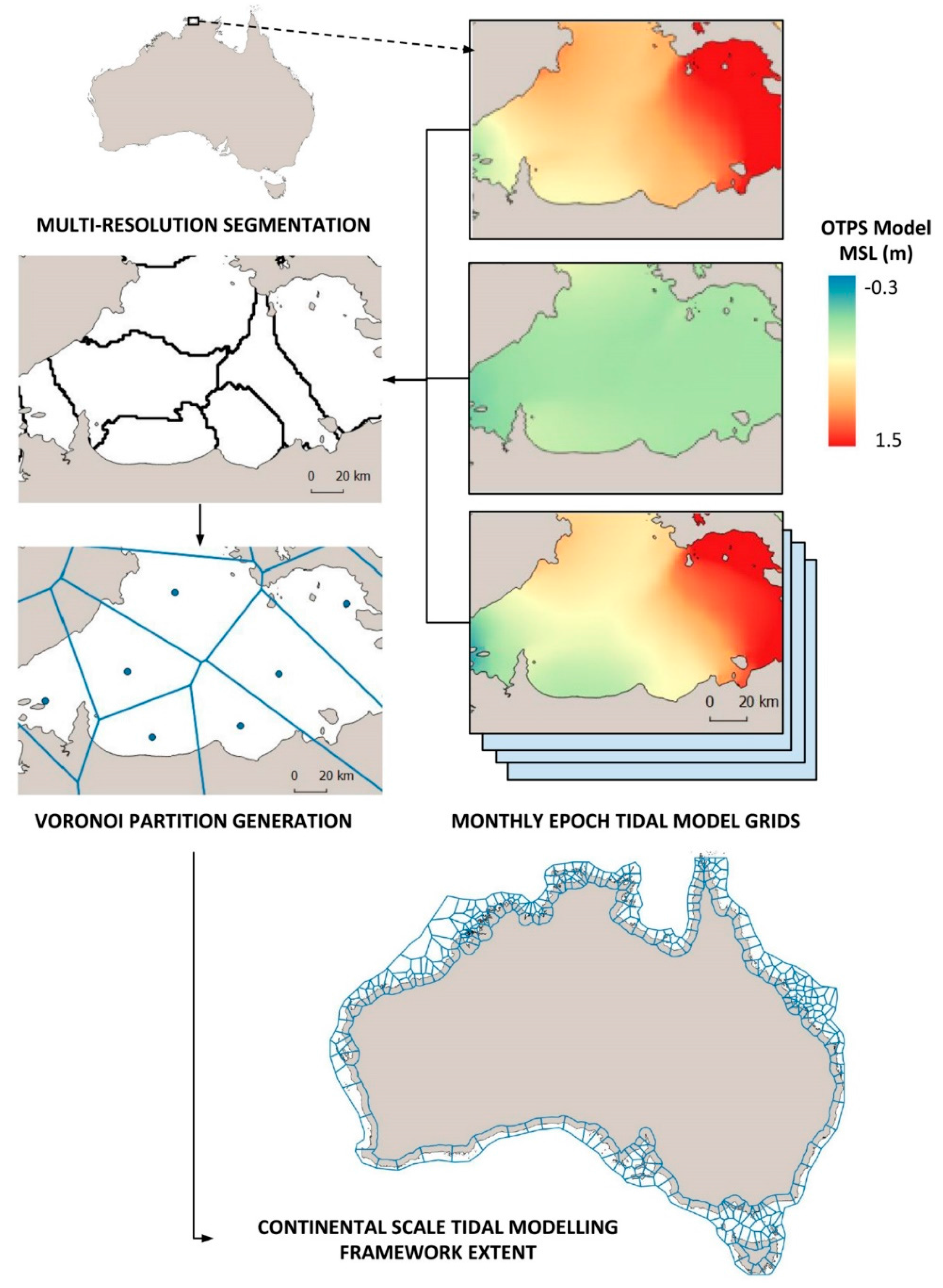
In this paper, we detail the development of a multi-resolution tidal modelling framework, underpinned by the concept of allowing the data to drive the scale and boundaries of the model. In moving away from the arbitrary boundaries of the ITEM tidal model, we are left with a variable spatial scale problem, defined by the global tidal model, and how its coarse resolution relates to the finer scale coastline features and processes. As noted by [
17], a single instantaneous tidal height value is always a simplification of a complex coastline or estuary. In this work, we use spatial segmentation and clustering partition methods to allow the spatial variability of the tidal model to drive the scale of the modelling framework, and therefore, minimise these simplifications.
To demonstrate the application of our framework to the creation of pixel-based composites, we utilise the geometric median (geomedian) approach of [
14]. This statistical method continues the concept of a data-driven approach, removing arbitrary scoring and choices in the compositing process. Case studies are presented, which include continental scale mosaics of the Australian coastline at high and low tide, and tailored examples demonstrating the potential of the tidally constrained composites to address a range of coastal change detection and monitoring applications. We conclude with a discussion on the potential applications of the composite products and method in the coastal and marine environment, as well as further development directions for the tidal modelling framework.
3. Results
3.1. Continental Scale Mosaics
To demonstrate the application of our tidal modelling framework at a continental scale, we have drawn upon the Landsat archive to produce 6-band pixel-based composites of the entire Australian coastline at high and low tide. These datasets are constrained not only by tide height, but also temporally, and show the geometric median surface reflectance for each pixel as observed over the selected time period. In order to draw out the full benefits that the geomedian composting approach can bring requires careful consideration and determination of the extents of both the temporal and tidal domains used.
3.1.1. Composite Domain Determination
The generation of clear, noise-free image composites is primarily influenced by two factors: the number and the quality of the input images. As the quality of single input images cannot usually be controlled (e.g., cloud cover, glint, noise); the relative number of input images usually provides a good estimation of composite quality. At each polygon extent, we are essentially determining the number of input images by modifying the ranges of both the temporal and tidal domains.
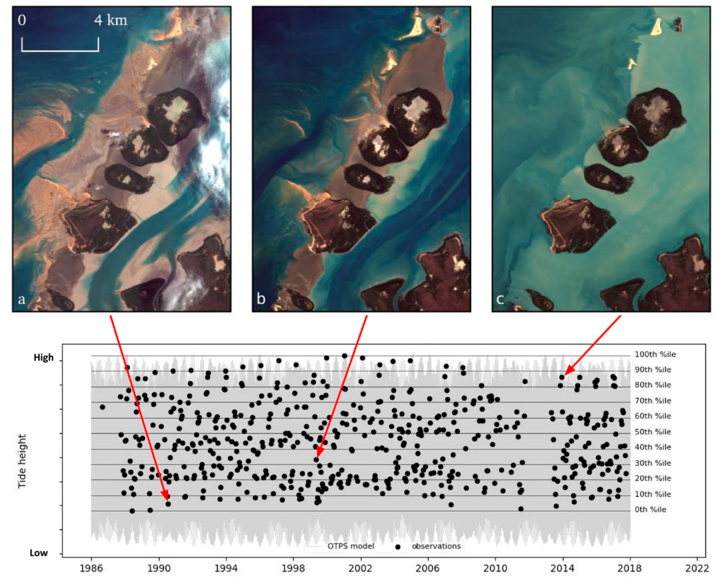
From a tidal perspective, to generate composites which reflect the coastal region at both high and low tide, we need to select images acquired as close to these extremes of the tidal range as possible. Complicating this requirement is the sun-synchronous nature of Landsat data acquisition, which means that all observations are made at approximately the same time of day (mid-morning in Australia) at any given location. Practically, this means that we are likely to only observe a limited subset of the full tidal range (
Figure 2), and the size and nature of the subset in any location will vary along with the different tidal regimes and ranges of the continent [
21]. Hence, we adopt the terminology used in [
16] using the observed tidal range (OTR), highest observed tide (HOT), and lowest observed tide (LOT) as distinct from common datums, such as lowest astronomical tide (LAT). For our continental scale application, we set the tidal range domain to the upper and lower 20th percentiles of the OTR, for the high and low tide composites respectively, and then use the temporal domain to further refine the composite quality.
In the temporal domain, a range of environmental and geographic factors need to be considered that influence the per-pixel and polygon data quality and archival completeness. For example, wet season cloud cover prevents high quality acquisitions for large parts of every year in some northern regions, while sun angle variations in different regions and seasons produce sun glint over water in many areas and lower reflected light values and increased noise in others (e.g., Tasmania). Many of these factors can be overcome by increasing the time range of observations fed into the composite process, however, this needs to be carefully balanced with the nature of the coastal environment in each polygon. In highly dynamic coastal regions, extending the time period results in a smoothing and generalisation of features; whilst in more static regions, such as coral reefs, the period can be extended and still maintain the crisp representation of features in the final composite.
With these considerations in mind, initial composites for each polygon were generated for the lowest and highest 20th percentile of the archive from 2010 to 2017. Each polygon composite was then examined for image quality (i.e., residual effects from persistent clouds or archival gaps). If the image quality was deemed poor, the nature of the coastal environment within the polygon was assessed, to determine if extending the time period would significantly smooth dynamic features and processes within the polygon. If extending the time period was deemed appropriate, a new composite was created with an additional 5 years of observations included, and the assessment process was repeated. In this way, we sought to create a balance in each polygon between composite image quality and utility of the composite imagery, to accurately capture all environments at high and low tide.
3.1.2. High and Low Tide Image Composites
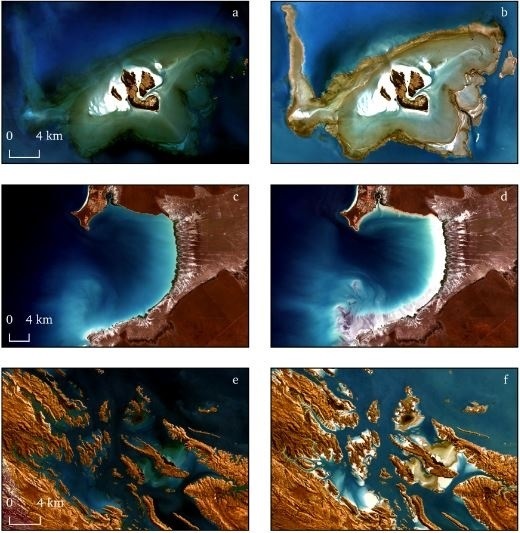
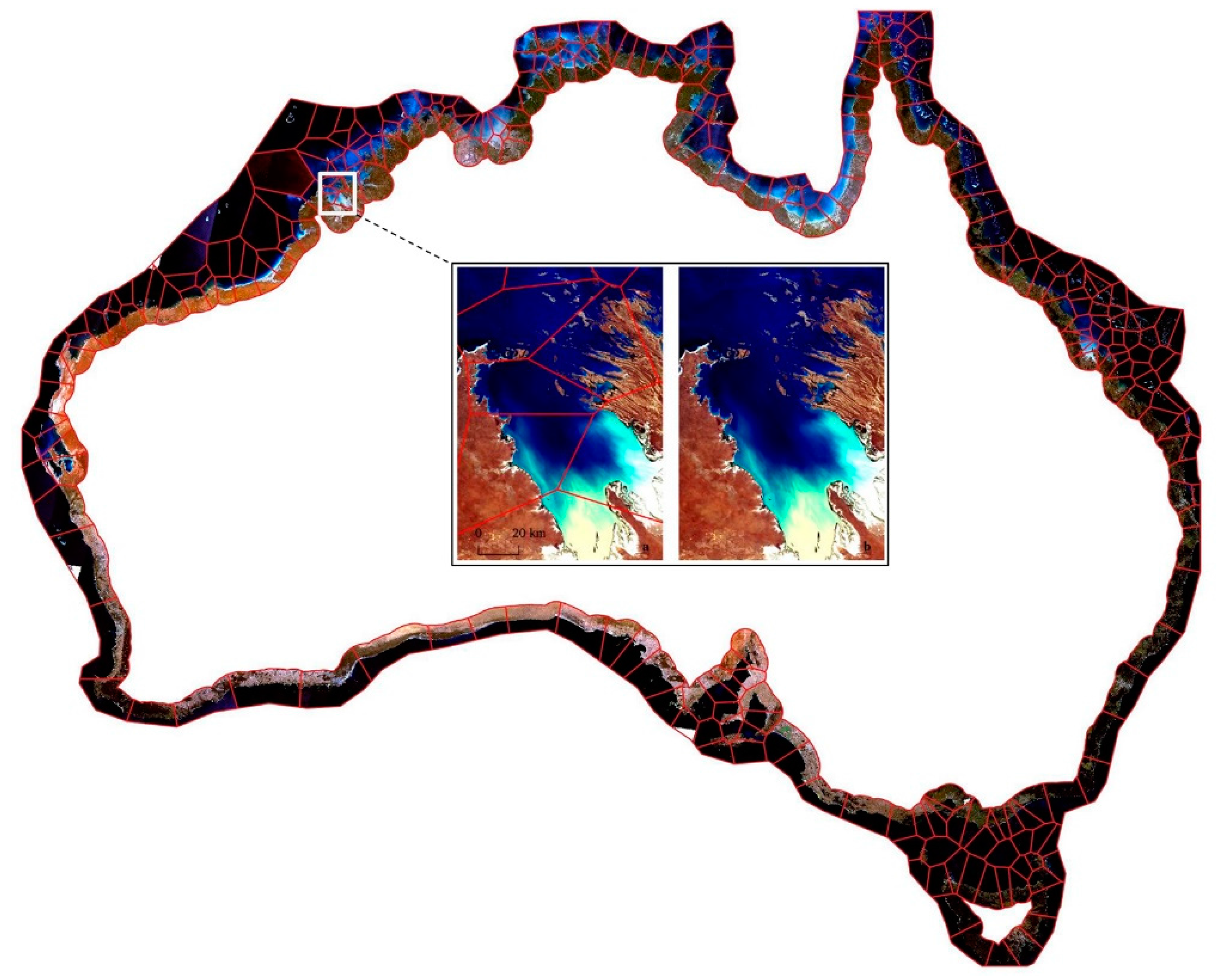
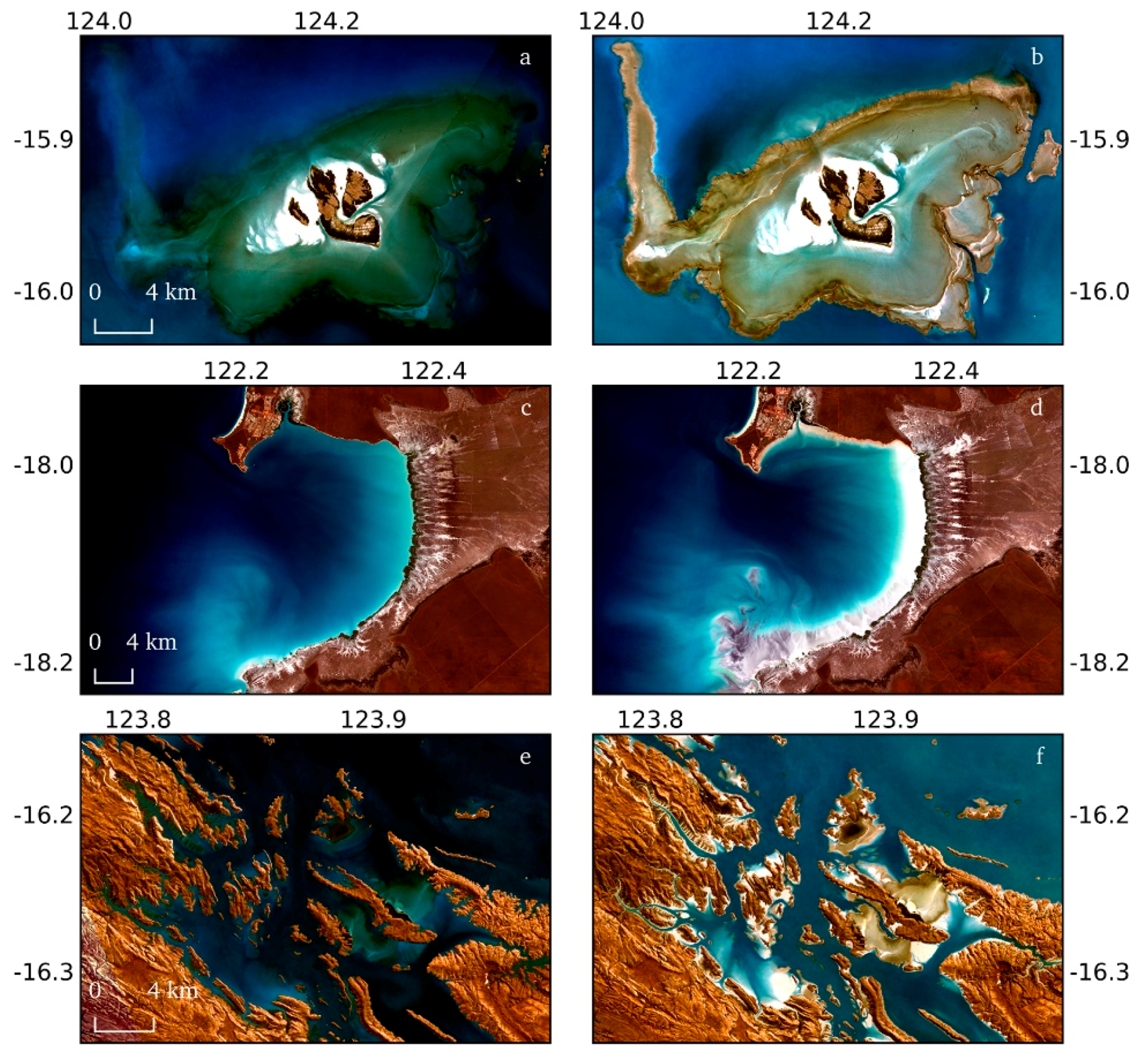
The resulting quality controlled geomedian images for each polygon are then mosaicked to produce the two continental scale multi-spectral composite image datasets, visualising the Australian coastline and reefs at high and low tide. The median properties of the process suppress noise from individual observations, producing a clean and noise free image that is highly interpretable for the delineation and identification of features and habitats. This also translates across boundaries of the mosaicked polygon sections, with smooth transitions, colour balance, and little indication of the original polygon footprints (
Figure 3). Not only are clouds and data gaps dealt with effectively as in terrestrial applications, but the suppression of glint, breaking water, and white-caps greatly increases the visual clarity and consistency of the images both in open water and coastal regions (
Figure 4).
In contrast to band independent statistical average methods, the geomedian preserves the band relationships within the modelled spectra at each pixel. This is important, as it opens up the opportunity to apply algorithms which incorporate field spectra for parametrisation or validation with more confidence and rigour. The ability to visualise and spectrally characterise the same environment at different biophysical stages (high and low tide) further extends the mapping and classification potential of the datasets.
3.2. Coastal and Estuarine Change
Producing clean and interpretable composites at a continental scale required a standardised approach, and often a long time-range of input data to counteract many of the regional effects in the greater dataset. By generating sequential composites in more localised applications, the process can also be used to discover, investigate, and monitor coastal change. Flexibility in how we define the domains for generating coastal composite imagery enables us to investigate two types of coastal change: change that is gradual, such as sediment transport or urban expansion, and change that is sudden, and caused by major events, such as floods and cyclones. By restricting inputs from the tidal domain, one of the major and confounding variables of change in the coastal zone is constrained, enabling a clearer understanding of the dynamics that are producing change. Similarly, modifications in the temporal domain can also be targeted to better characterise the approximate date or rate of change.
In the following sections, we look at these two types of change, and ways in which the composite domains can be targeted to assess them. Firstly, we show how time series composites can be generated using a consistent time step to highlight average change over time, and how they are useful in environments where change is likely to be gradual and ongoing. Second, we show how composite time series can be generated using major events to dictate the temporal inputs to the composites, and we demonstrate the importance of the tidal domain in this type of analysis.
3.2.1. Natural Change Utilising Consistent Time Steps
Dynamic regions of the Australian coast and their associated change can be identified in composites that span the length of the Landsat archive using a consistent time step. Although each geomedian composite depicts an averaged representation from the input ensemble of images, consistent time step composites can be useful to indicate whether the rate of change is constant across the whole time series, and can identify periods of noteworthy change.
Two approaches can be used in the identification of coastal change study sites: (1) regions are located based on a prior understanding of the local change conditions, or (2) a data driven approach can be used to identify dynamic coastal areas. The latter approach has been used successfully in this work to identify change locations in remote regions of Australia.
The data driven approach utilises the Intertidal Extents Model (ITEM) v.1 confidence layer [
16] as a diagnostic tool. The confidence layer was designed to highlight any errors in the original tidal modelling framework, although as shown in [
16], the layer also has the ability to indicate areas of potential coastal change and instability. This is because it highlights pixels where changes in a land or water classification do not correspond with the underlying tidal model, indicating that other dynamics are driving the change.
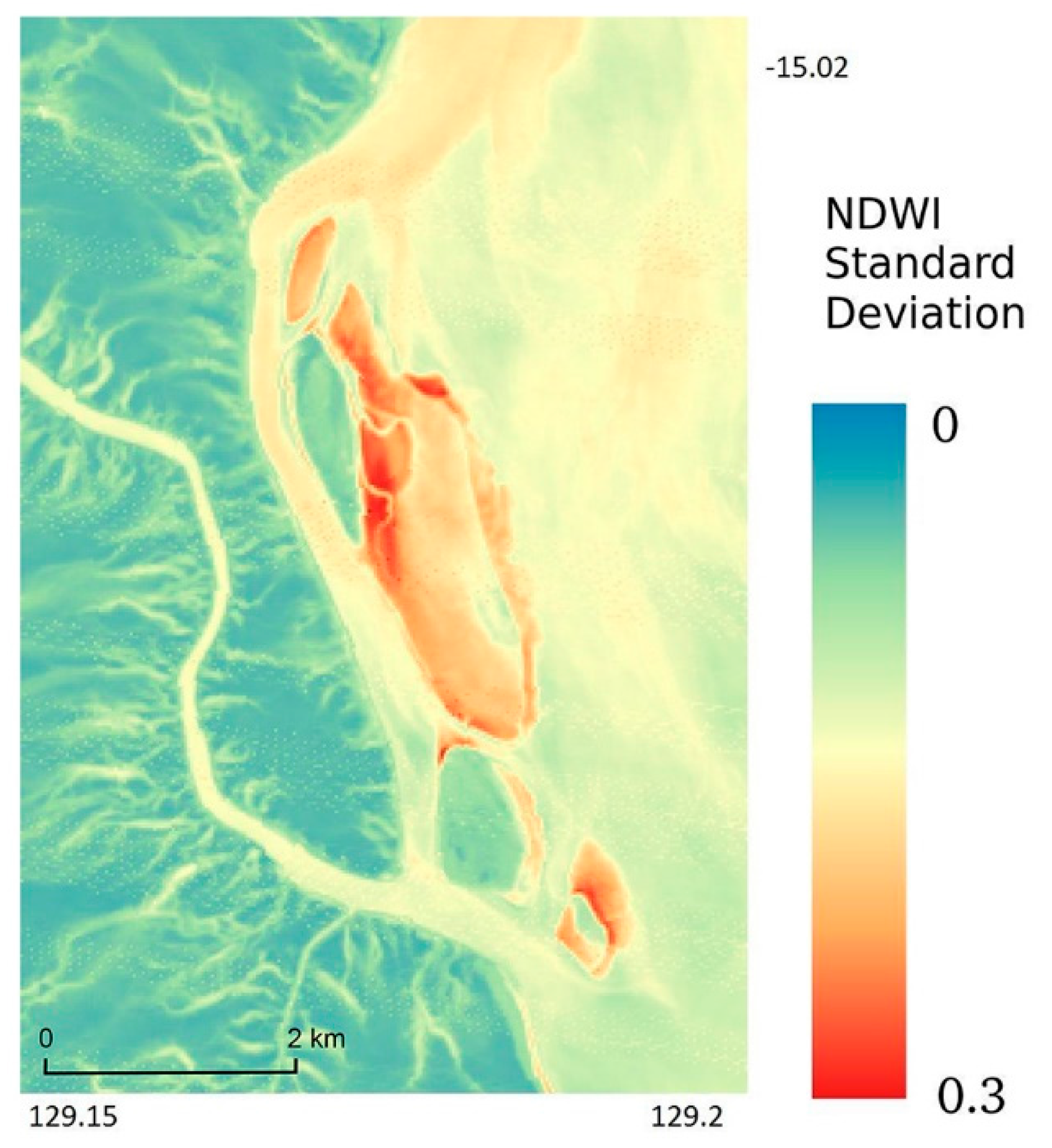
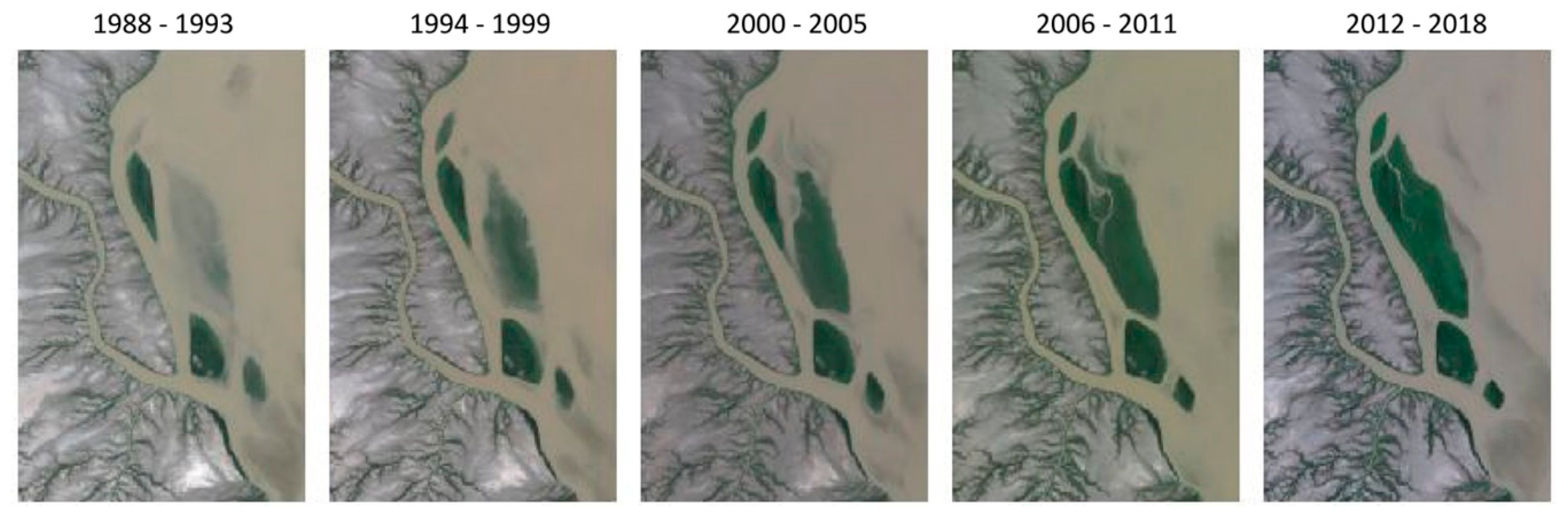
The data driven approach to identifying change locations revealed that the Keep River in Australia’s Northern Territory has a number of sites where significant geomorphic change was identified during the recorded history of imagery for the site (
Figure 5). Whilst the ITEM confidence layer does not indicate the timing and nature of the change, or whether it was event based or naturally continuous, this can be further explored using consistent time step composites.
To investigate changes indicated in
Figure 5, images of the mid-tide range (40th to 60th percentiles of observed tide heights) were used as inputs to the geomedian composite process, with 6 year epoch time steps defined across the length of the archive. Using the mid-tide range reliably provides a rich dataset from which to select input images, without a dependency on the less frequently occurring observations at the extremes of the tidal range. The time series of 6 year composites for the Keep River (
Figure 6) show two processes of natural change occurrence. Firstly, the area is seen to be dynamic in terms of sediment transport with banks both continuously forming and disappearing. Overall, sediment deposition and the development of the observed sand/mud banks appear to be the dominant driver of change in this environment. Secondly, the formation and settlement of these banks has been the catalyst for the progression of vegetation (mangrove) in this part of the river.
3.2.2. Event Based Change Utilising Ancillary Data
Event based coastal change was investigated by creating geomedian composites where the temporal domain steps are informed by an ancillary data source; in this case, the flood water heights from in situ gauge measurements. Flood gauge measurements for the Burdekin River, Queensland, were sourced from the Bureau of Meteorology [
29], indicating a number of significant events over the period covered by the Landsat archive in the DEA.
The Burdekin River is one of Queensland’s largest rivers, draining a catchment dominated by livestock grazing as the primary land use [
30]. Discharging into the Coral Sea, and occasionally, the Great Barrier Reef, it is well documented to transport high sediment loads from catchment to shore [
31]. It is also susceptible to seasonal cyclones and subject to major semi-regular flooding, often as a consequence of the weather systems associated with the annual cyclone season [
32].
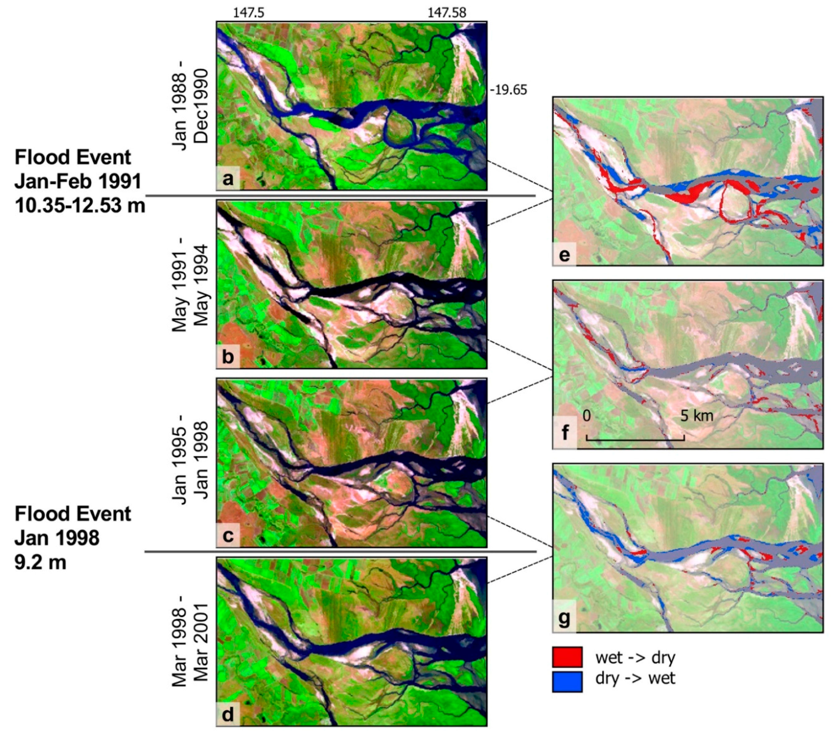
The Burdekin River estuary is a multi-channel system where geomorphic change is evident in the 30 year imagery archive of the DEA. To investigate whether composite imagery can indicate that these changes can be attributed to flooding events, we generated geomedian composites at 3 year time steps either side of flood events in 1991 and 1998 indicated in the gauge record. These composites were constrained to the lowest 20% of the OTR to allow the maximum substratum extent to be exposed across the estuary. A simple land/water classification, identical to that used in [
16], was completed on each composite image, utilising the normalised difference water index (NDWI) [
33]. Differencing of the land and water extents between subsequent composites was then completed to indicate areas of change from wet to dry and vice versa (
Figure 7).
This analysis shows that that geomorphic change in the estuary is influenced considerably more by flood events, rather than by regular flow. For example, the change shown on either side of both the 1991 (
Figure 7e) and 1998 (
Figure 7g) flooding event is significantly greater than that of the subsequent comparable time periods where no flood event is recorded (
Figure 7f).
There are two notable strengths provided by the tidal tagging and geomedian compositing approach to change detection applications. Firstly, the noise suppression and reduced pixel-to-pixel variation in the composites enables both improved visual interpretation and a cleaner application of indices and classification techniques. Secondly, change effects related to the tidal influences can be largely eliminated from change detection analyses. We can clearly illustrate the importance of this second feature of the method using the Burdekin River case study.
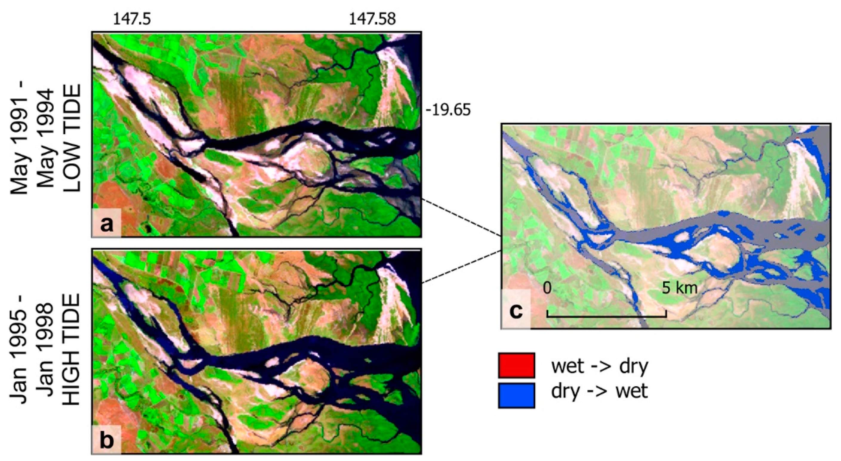
The Burdekin River case study was generated using imagery identified from the lowest 20% of observed tide heights for each of the time series epochs. If the tidal domain ranges were varied between these epochs, we would expect the tidal influences to confound and hinder the detection of geomorphic change. To demonstrate, we select a non-flooding comparison period between the years of 1991 to 1994, and 1995 to 1998, shown in the low tide case study as
Figure 7b,c,f. In
Figure 8, we show the same analysis performed on the same epochs, but using a composite created from the highest 20% of the OTR for the latter period. As expected, a significant degree of change was detected (
Figure 8c) that can be almost entirely attributed to tidal effects when compared to
Figure 7f, where change is assessed between two composites of comparable tidal ranges. This is an extreme example, drawing imagery for both ends of the tidal range to illustrate the concept, and one might argue that a user would naturally select images from comparable tidal stages for this type of analysis. However, to do so would require moving back to the single scene analysis paradigm, and the associated environmental noise and cloud issues that accompany it. By developing a framework to incorporate tidal tagging and composite generation, we are providing a method to leverage the benefits of image compositing in this highly dynamic environment.
4. Discussion and Future Work
In
Section 3.1, we have shown how our developed tidal modelling framework can be applied at a continental scale to produce a clean, cloud and glint free composite mosaic for the full Australian coastline and the Great Barrier Reef at high and low tide. The characteristics of the geomedian approach ensure that the resulting mosaic is visually appealing, suppressing temporal and pixel-to-pixel noise. The smooth transitions in the mosaic between the individually processed image polygons also indicate that when combined with the geomedian process, our spatial characterisation of the tidal model is at an appropriate scale to capture its variability, whilst striking a balance with the computational demands of processing 30 years of Landsat data at a continental scale. In our process, we aimed to use tidal data to drive the spatial structure of the model, although ultimately, some manual decisions were required (e.g., scale of the segmentation, coastal alignment of Voronoi boundaries) for practical implementation. Ideally, a fully data driven approach, such as under a Bayesian framework (e.g., [
34]) might be adopted to optimise the spatial dimension of the model.
The reduced noise and spatial consistency of the mosaic greatly increase its interpretability, and therefore, its utility to be paired with shoreline and change detection algorithms. The ability to switch between and modify the temporal and tidal domains in our framework further increases its functionality and potential for more targeted change detection applications, a selection of which we have demonstrated in
Section 3.2. With the analytical and computing capacity provided by the DEA, there is potential to build these open source algorithms into a user-friendly interface, where the user can modify the location, temporal and tidal variables in the composite generation process to target their specific needs. The flexible nature of the developed frame work and the DEA means that in the near future, the user will not only be able to access the vast archive of Landsat data, but also data from new sensors such as Sentinel-2, greatly increasing the density of the archive and allowing finer temporal steps and analysis. However, combining the data from these sensors to allow calibrated time series analysis and composite generation presents a number of challenges, including radiometric calibration, atmospheric correction, and spatial registration [
35], and is an active area of research internationally [
36,
37].
One of the most significant benefits of using the geomedian approach for creating composites is the maintenance of the spectral relationship between bands. As we have noted, this increases the potential utility of the composites for processes such as band ratios, machine learning, and classification algorithms. For instance, the mapping of mangrove of extents was explored by [
38] using band-independent median mosaics of Landsat data at high and low tide. The classification in their work was restricted to samples generated from the synthetic composites, based on pre-defined regions of interest. With geomedian spectra, this kind of work can be extended to utilise in situ and reference spectral endmembers for classification, instead of requiring some prior knowledge of habit extent, whereas this type of approach is not valid with band independent statistically derived composites.
In the marine space, the spectral characteristics of the geomedian open up the possibility for temporal and tidally constrained composites to be used for a range of water quality and parameter estimation problems. Future work will investigate the application of a recently developed turbidity algorithm shown to be applicable at a global scale with Landsat data [
39,
40]. The implications of applying this approach to composite data will be explored, where the domains can be tailored seasonally, as well as drawing further information from the tidal modelling process by sorting images based on tidal phase (i.e., ebb or flow tide).
The development path of the tidal modelling framework is a direct result of insights gained from the implementation of original tidal tagging process used in the ITEM product [
16]. The workflow of that product makes it possible for straightforward implementation of the new multi-resolution framework for tidal tagging, and work is underway to assess the improvements that this is bringing to version 2 of the ITEM. Incorporated in this proposed work is validation of both the ITEM product suite and the new tidal modelling framework, with a combination of in situ GPS elevation and tidal gauge measurements. This is aimed at providing increased confidence in the full range of products that can be realised through the tidal modelling and composite creation tools on the DEA platform.
5. Conclusions
In this paper, we have presented a methodology for generating pixel-based composites from large time series of earth observation data in highly dynamic coastal regions. The tidal modelling framework to enable this process was developed from a global tidal model, and by allowing the model itself to define the spatial variability by which we query the data, the framework allows the confounding tidal influence in coastal regions to be constrained. In the examples presented, we show the capability of the method to generate clean, noise free composite mosaics of the Australian coastline at high and low tide, and we demonstrate how the framework can be tailored to address a range of change detection applications.
To fully realise the potential of the method, there remains challenges to be addressed, including the ability to integrate data from a range of sensors. The potential of further refining how the tidal modelling is completed is also discussed, with the aim of moving to a fully data driven approach not requiring manual decision processes. One of the important areas of future work identified centres around the properties of the compositing method that preserves the band relationships within the pixel composite spectra. This feature provides the potential to apply a range of spectral analysis processes, such as classification and empirical parameter estimation, in a more robust manner when compared to band-independent statistical composites.

