Article

New Tropical Peatland Gas and Particulate Emissions Factors Indicate 2015 Indonesian Fires Released Far More Particulate Matter (but Less Methane) than Current Inventories Imply

1
King’s College London, Department of Geography, Strand, London WC2R 2LS, UK
2
NERC National Centre for Earth Observation (NCEO), King’s College London, London WC2R 2LS, UK
3
Center for International Forestry Research, Jl. CIFOR, Situgede, Bogor 16115, Indonesia
4
King’s College London, School of Population Health & Environmental Science, Strand, London WC2R 2LS, UK
5
Royal Netherlands Meteorological Institute, 3731 De Bilt, The Netherlands
6
Department of Geophysics and Meteorology, Bogor Agricultural University, Kampus Darmaga, Bogor 16680, Indonesia
7
Indonesian Agency for Meteorology, Climatology and Geophysics (BMKG), Jakarta 10610, Indonesia
8
Institute of Geography, Soil Science/Soil Ecology, Ruhr-University Bochum, Universitätsstrasse 150, 44801 Bochum, Germany
9
Leibniz Institute for Agricultural Engineering and Bioeconomy, Max-Eyth-Allee 100, 14469 Potsdam, Germany
*
Author to whom correspondence should be addressed.
Remote Sens. 2018, 10(4), 495; https://doi.org/10.3390/rs10040495
Submission received: 31 January 2018 / Revised: 5 March 2018 / Accepted: 19 March 2018 / Published: 21 March 2018

Abstract

:
Deforestation and draining of the peatlands in equatorial SE Asia has greatly increased their flammability, and in September–October 2015 a strong El Niño-related drought led to further drying and to widespread burning across parts of Indonesia, primarily on Kalimantan and Sumatra. These fires resulted in some of the worst sustained outdoor air pollution ever recorded, with atmospheric particulate matter (PM) concentrations exceeding those considered “extremely hazardous to health” by up to an order of magnitude. Here we report unique in situ air quality data and tropical peatland fire emissions factors (EFs) for key carbonaceous trace gases (CO2, CH4 and CO) and PM2.5 and black carbon (BC) particulates, based on measurements conducted on Kalimantan at the height of the 2015 fires, both at locations of “pure” sub-surface peat burning and spreading vegetation fires atop burning peat. PM2.5 are the most significant smoke constituent in terms of human health impacts, and we find in situ PM2.5 emissions factors for pure peat burning to be 17.8 to 22.3 g·kg−1, and for spreading vegetation fires atop burning peat 44 to 61 g·kg−1, both far higher than past laboratory burning of tropical peat has suggested. The latter are some of the highest PM2.5 emissions factors measured worldwide. Using our peatland CO2, CH4 and CO emissions factors (1779 ± 55 g·kg−1, 238 ± 36 g·kg−1, and 7.8 ± 2.3 g·kg−1 respectively) alongside in situ measured peat carbon content (610 ± 47 g-C·kg−1) we provide a new 358 Tg (± 30%) fuel consumption estimate for the 2015 Indonesian fires, which is less than that provided by the GFEDv4.1s and GFASv1.2 global fire emissions inventories by 23% and 34% respectively, and which due to our lower EFCH4 produces far less (~3×) methane. However, our mean in situ derived EFPM2.5 for these extreme tropical peatland fires (28 ± 6 g·kg−1) is far higher than current emissions inventories assume, resulting in our total PM2.5 emissions estimate (9.1 ± 3.5 Tg) being many times higher than GFEDv4.1s, GFASv1.2 and FINNv2, despite our lower fuel consumption. We find that two thirds of the emitted PM2.5 come from Kalimantan, one third from Sumatra, and 95% from burning peatlands. Using new geostationary fire radiative power (FRP) data we map the fire emissions’ spatio-temporal variations in far greater detail than ever before (hourly, 0.05°), identifying a tropical peatland fire diurnal cycle twice as wide as in neighboring non-peat areas and peaking much later in the day. Our data show that a combination of greatly elevated PM2.5 emissions factors, large areas of simultaneous, long-duration burning, and very high peat fuel consumption per unit area made these Sept to Oct tropical peatland fires the greatest wildfire source of particulate matter globally in 2015, furthering evidence for a regional atmospheric pollution impact whose particulate matter component in particular led to millions of citizens being exposed to extremely poor levels of air quality for substantial periods.

Graphical Abstract

1. Introduction

1.1. Landscape Burning in Southeast Asia

Smoke from landscape fires is a significant environmental health issue in parts of southeast Asia, where burning is used routinely to clear unused lands (forest and scrub) before planting, to remove post-harvest crop residues prior to re-planting rapidly and cheaply, or even as a weapon in land disputes [1,2]. Comprised of a mixture of greenhouse gases (GHGs) and air pollutants [3,4,5], the smoke impacts are most keenly felt during dry spells in Indonesia, which hosts more than 80% of SE Asia’s carbon-rich tropical peatlands [6,7]. Peat deposits can exceed twenty meters depth in places [6,7,8], having formed over millennia via the reduced decay of forest litter. Over the last 50 years, deforestation and the construction of drainage canals, largely to support agriculture, has increased the flammability of large areas of Indonesia’s tropical peatlands compared to their naturally moist state, and during dry spells drained peat can dry sufficiently to be ignitable by surface vegetation burning [9,10,11]. The resulting fires can propagate vertically downward into the peat as well as laterally across the landscape [9], generating potentially very large areas of simultaneous burning [1,11,12], with fuel consumptions per unit area perhaps two orders of magnitude higher than most other landscape fire types [13,14]. Burning these fossil carbon stores releases very significant amounts of the greenhouse gas carbon dioxide [8,12,15], while the predominantly smoldering phase combustion also maximizes production of the strong greenhouse gas methane [12,16], gaseous air pollutants such as carbon monoxide, ammonia, hydrogen cyanide and formaldehyde [16,17,18,19], as well as fine particulate matter (PM) [16,17,18,19]. This latter smoke constituent, locally termed “haze”, is the one having most direct relevance to short-term human health [20], and it can also remain in the atmosphere for days or weeks and be subject to long-range transboundary transport to affect citizens far from the fires themselves [21,22].
The extreme 2015 El Niño lead to drought and the most severe Indonesian fire season since 1997, with major international concerns related to greenhouse gas (GHG) releases [12] and biodiversity loss [23]. In line with increasing anxieties related to wildfire smoke exposure [21,22,23,24], there were also serious concerns regarding air quality impacts on human health [25]. With a few notable exceptions [3,26,27,28,29], health has typically received far less international attention than the climatological implications of El Niño-related SE Asian biomass burning, though recently atmospheric chemical transport models (CTMs) have been used alongside particulate emissions estimates to begin to assess the regional health consequences of fine PM exposure [26,30,31]. Wildfire smoke particles have a size distribution typically peaking well within the 2.5 μm particle diameter range [20], small enough to pass into the human respiratory system [32].
Wildfire PM2.5 emissions estimates for input into CTMs are generally calculated by combining mapped fuel consumption rates (g·m−2·s−1) with PM2.5 emissions factors (g·kg−1), but while satellite-based approaches to estimate fuel consumptions are becoming increasingly available and/or mature [33,34,35,36], until recently the only particulate (or indeed gaseous) emissions factors (EFs) available for tropical peatlands came from a few laboratory burns of peat samples, and these showed significant and unexplained intra-sample variability [16,37]. Emissions factors derived from laboratory burning may also not be fully representative of true landscape fires [38], especially the type of extreme fire conditions seen in Indonesia in 2015, which included large and intense forest fires flaming atop burning peat [12]. Only in situ sampling of smoke from real landscape burning can likely deliver emissions factors representative of such conditions, and at the height of the 2015 Indonesian fires a subset of the current authors made the first tropical peatland fire emissions factor measurements based on field sampled data, focusing on the primary emitted gases CO2, CO and CH4 [12]. The in situ EFs derived from these data were significantly different to those seen in laboratory peat burning, especially in relation to carbon monoxide and methane, and these findings were soon followed by [39] whose in situ EFs included a far wider range of gaseous species as well as particulates. Here we add significantly to these works, reporting further detailed EFs for tropical peatland fires that are based on in situ measurements of PM2.5, black carbon, CO2, CO and CH4, made both in smoke from pure peat fires and the combined burning of vegetation atop peat, including extremely intense forest burning. We both update the prior gas-only EF’s presented in [12], extend to particulates, and use methods different (and complementary to) those of [39]. We use our new gaseous emissions factors and in situ peat carbon content measurements made at the fire sites to update satellite-derived estimates of Indonesian fuel consumption [12], combine these with our EFPM2.5 measures to estimate fine particulate emissions, and use new very high temporal resolution fire radiative power (FRP) data from geostationary satellites [40] to understand the emissions variability over both individual days and over the fire event itself in more detail than ever before (hourly temporal resolution, 0.05°). We also assess the landscape and physio-chemical peat properties of our field sampling sites to help determine factors that may regulate EF variability, and we compare our total dry matter fuel consumption and smoke emissions estimates to those provided by other widely-used global fire emissions inventories. Prior to these analyses, we first put the atmospheric impact of the 2015 fires into context using data from Indonesia’s national air quality monitoring network.

1.2. Indonesian Peatland Fires and Air Quality in 2015

Using satellite FRP and atmospheric carbon monoxide (CO) total column concentration retrievals, along with tools developed within the Copernicus Atmospheric Monitoring Service (CAMS), it has been previously estimated [12] that 336 ± 99 Tg of peat were consumed in the extreme September and October 2015 Indonesian fires, along with ~52 Tg of vegetation. Satellite imagery (Figure 1a) and Indonesia’s air quality monitoring network (Figure 1b,c), provide stark evidence of the enormous atmospheric impacts of the emitted smoke. Palangkaraya, the capital of Central Kalimantan (pop. 250,000) showed the greatest air quality impact, and daily average PM10 concentrations often reached 1000 to 2000 μg·m−3 (Figure 1b), far exceeding those reported downwind of organic soil burns elsewhere [41]. To our knowledge this represents perhaps the worst sustained air quality ever recorded worldwide, with levels shockingly higher than the 50 μg·m−3 short-term (24-h) exposure limit set by the World Health Organization (WHO), and far beyond even the 300 μg·m−3 judged by the Singapore National Environment Agency (NEA) to be “extremely hazardous”. Figure 2a shows the severe reduction in visibility experienced in Palangkaraya, and these types of extreme atmospheric impacts were repeated to varying degrees across the region [42].

2. Methodology

2.1. Field Sampling Approaches

To derive particulate emissions factors based on direct in situ measurements we sampled smoke at five fixed measurement locations, representing a variety of landscape types and fire behaviors in the region primarily southeast of Palangkaraya (Figure 3; Table 1). PM2.5 makes up the clear majority of the PM10 mass in biomass smoke [20], with [43] suggesting >90% in Southeast Asian haze, so we focused on derivation on PM2.5 emissions factors as both the dominant particulate component and that of most relevance to human health [3,4]. At Locations 1, 2 and 4 (Figure 3; Table 1) close-to-source, point-based sampling of gas and particulate emissions was conducted directly (1–5 m distance) where sub-surface peat burning was delivering smoke through surface cracks and gaps (Figure 2b). At these locations, occasional surface (sometimes flaming) combustion of minor amounts of residual dead vegetation added to the sampled smoke, and was noted when it did so. At Locations 3 and 4, point-based sampling of smoke coming from spreading vegetation fires atop burning peat was conducted at greater distances (>200 m) from the source (due to safety concerns) (Table 1). Figure 3 shows satellite imagery captured close to the time of these field measurements, and at all but Location 3 were able to sample the physio-chemical composition of the peat fuel as well as the smoke itself, in order to investigate potential controls on emissions factor variability.

2.1.1. Smoke Measurements at Fixed Locations

At each fixed measurement location, smoke plume PM2.5 concentrations were recorded at 1 Hz using a TSI DustTrak™ DRX laser photometer (as deployed for biomass burning studies by e.g., [44,45]). The DustTrakTM was fitted into a modified version of the aerosol sampling box described in [45], with an isokinetic flow splitter (TSI 3708) directing the airflow to different measurement pathways and Casella Apex Pro pumps providing the makeup flow to ensure correct size separation in the PM2.5 inlet (BGI miniPM® inlet 5011, 5 L·min−1). Smoke black carbon (BC) content was assessed using a microAeth AE51 [46].
The DustTrakTM measures via the near-perpendicular particle scattering of a 780-nm laser diode beam, and is factory-calibrated to give PM mass concentrations using the respirable fraction of standard ISO 12103-1 A1 test dust (so-called Arizona road dust). DustTrakTM readings made during applications where the dominant particulates have densities divergent from those of this A1 test dust material require application of a re-calibration factor, usually derived through linear regression of contemporaneously collected DustTrakTM data and co-located gravimetric PM measurements [47,48]. Our application requires this, and our recalibration factor was based on simultaneous PM2.5 samples collected on pre-weighed 25 mm Emfab filters (Pall Corp., New York, NY, USA; Type: EMFAB TX40HI20-WW; Part No.: 7221) which we located within the aerosol sampling box so as to sample the same incoming air as the DustTrakTM.
Following [45], simultaneous, co-located trace gas measurements were made to enable the 1 Hz DustTrakTM PM2.5 concentration data to be converted into EFPM2.5 estimates. We recorded both CO and CO2 (along with CH4 and H2O), to enable separation of periods of flaming and smoldering combustion based on the plumes modified combustion efficiency (MCE) [49]. A high-precision, cavity enhanced laser absorption spectrometer ([50] (supplied by Los Gatos Research-LGR, San Jose, CA, USA) was used to measure all four gases simultaneously, increasing measurement performance and avoiding many of the limitations found when using multiple lower-cost sensors having differing sensor response times for each gas species [45,51]. At the 1 Hz sampling rate used, trace gas measurement precisions were 2.63 ppm (CO2), 0.14 ppm (CO) and 1.71 ppb (CH4) [Allan variance, 1 sigma @ 1 Hz], with a total absolute concentration uncertainty of 1%.
PM2.5, BC and trace gases were measured at each fixed location listed in Table 1 for 40–90 min, with a variety of plumes sampled as wind direction changed and apparatus re-positioned (see Plumes 1 to 12 in the timeseries shown in Figure 4). Simultaneously with the co-located PM2.5 and trace gas measures, remote sensing of the smoke from the wider combustion zone was conducted using an open path (OP) Fourier Transform Infrared (FTIR) spectrometer-based “Air Monitoring System” (MIDAC Corporation, Irvine, CA, USA). The spectrometer was sited to view through the plumes and towards a ~1275 °C silicon carbide glower-based IR source, placed at the focus of a gold-plated aluminum reflector around 20 m to 50 m distant from the spectrometer itself, as detailed in [52]. Data collected outside of the plumes provided background samples, albeit of still heavily polluted air.
Finally, to provide measurements more representative of spatial variations in background “haze” and occasional very large ground-level plumes, sampling of PM2.5, BC and trace gases was also undertaken along a 240 km long, 9-h vehicle transect conducted from the southern coast (Banjarmasin) to the interior (Palangkaraya) on 11 October 2015, close to the peak date of fire activity and using the same aerosol sampling box and laser absorption spectrometer as deployed at the fixed measurement locations (see Section 3.5 for details of the transect route).

2.1.2. Physio-Chemical Measurements of Peat

At each fixed measurement location (bar Location 3), samples of unburned peat from areas neighboring the active combustion zone were collected, sampling three places at each location and at multiple depths (0–10 cm and 10–30 cm, plus wherever it existed at the very surface (O horizon)). Most soil hollows formed by peat burning are less than 30 cm deep [9,14], and waterlogged conditions were often found below this depth. Gravimetric moisture content was calculated by drying peat samples to constant weight at 40 °C (to avoid loss of readily available organic matter), and carbon (C), nitrogen (N) and hydrogen (H) contents were assessed using a Carlo-Erba Model 1108 Elemental Analyser. Subsequently, air-dried peat samples were subject to spectral absorbance analysis (350–2500 nm spectral range) to identify specific functional groups present in the organic matter.

2.2. Atmospheric Data Processing

2.2.1. Point-Sampled Data (DustTrak™ and Laser Absorption Spectrometer)

All 1 Hz data were first sub-sampled to 0.125 Hz to avoid our analyses being impacted by autocorrelation effects stemming from non-negligible sample exchange times within the instruments measurement chambers. Excess concentrations for each smoke constituent (x) (i.e., Δx) were calculated via subtraction of the first percentile of the non-plume measurements, representing the best estimate of non-plume background concentrations (see example timeseries in Figure 4). Modified combustion efficiency (MCE) was calculated using Equation (1) at times when plumes were being sampled (taken as periods when ΔCO ≥ 6 ppm):
MCE = Δ CO 2 Δ CO 2 + Δ CO
MCE broadly separates smoke into smoldering-dominated (MCE < 0.9) and flaming-dominated (MCE ≥ 0.9) [20], and an example time-series for Location 1 is shown in Figure 4.
By basing our emissions factor calculations [Equation (1)] on emission ratios (ERs), derived as the slope of the ordinary least squares (OLS) linear best fit to scatterplots of the laser absorption spectrometer data for each plume (see examples for Plume 1, Location 1 in Figure 5), the derived EFs are insensitive to inaccuracies in the assumed background concentrations, as explained by [52].
E F x = 1000 · F c · M M x M M c ( E R x / CO 2 j = 1 n N C j · E R j / CO 2 )
where ERx/CO2 is the emission ratio of gas x to CO2 (mol−1·mol−1), Fc is the fractional carbon content of the peat (unitless), MMx is the molecular mass of species x (g), 1000 g·kg−1 is a unit conversion factor, MMc is the molecular mass of carbon (12 g), NCj is the number of carbon atoms in compound j, and the sum in the denominator is conducted only over the three primary carbonaceous gases (CO2, CO and CH4) that together account for more than 95% of total smoke carbon [38,53,54], inflating the derived EFs by a few percent at most compared to if all carbonaceous species were included [55].
The DustTrak™ data had the filter-based recalibration factor applied in order to deliver accurate peat fire smoke PM2.5 concentrations (µg·m−3) (see Section 3.2). The re-calibrated data were used to derive two independent estimates of each plumes PM2.5 emissions factor, based respectively on the PM2.5 mass concentrations and the simultaneous CO and CO2 measurements following the approach of [45]:
E F PM 2.5 CO = aER Δ PM 2.5 / Δ CO × EF CO
E F PM 2.5 CO 2 = bER Δ PM 2.5 / Δ CO 2 × EF CO 2
where ERΔPM2.5/Δx is the ratio of PM2.5 to gas x, and a and b (µg·m3)−1 are unit conversion factors.
Because of the approximately 6× longer sample exchange time of the laser spectrometer compared to the DustTrakTM, the temporal width of each smoke plume is typically wider in the trace gas record than in the PM2.5 data (see Figure 4 example), a characteristic that can lead to potential emissions ratio (and thus emissions factor) biasing if unaccounted for. “Plume-integrated” approaches of the type often used during airborne campaigns [56] have been shown to be more effective than fixed interval averages when adjusting for this effect [51], and per-plume ERΔPM2.5/ΔCO2 and ERΔPM2.5/ΔCO measures were derived from our data using integrated amounts of each species assessed across the duration of each plume. The two emissions ratios were then used to calculate two separate PM2.5 emissions factors using Equations (3) and (4).
An alternative approach to ‘plume integrated’ ER derivation was used to confirm the insensitivity of the derived emissions ratios to the precise delineation of the individual plumes. This confirmation was required because the partitioning into plumes was somewhat subjective and based on patterns in the data and visual observations of the times when recently emitted smoke intercepted the sampling inlet of the smoke measurement system (see Plumes 1 to 12 in Figure 4). This alternative approach to emissions ratio derivation is detailed in [57], and is commonly applied during studies of ambient air quality [58]. It defines the ER of two targeted atmospheric species via a reduced Major Axis Regression (RMA) of three individual, temporally consecutive species concentration measures, moving through the entire time-series and taking the mode as the final emission ratio [59]. Unlike the plume-integrated approach, this second method of ER derivation does need to take explicit account of the differing sensor response times of the laser spectrometer and DustTrakTM instruments, and so prior to its application the re-calibrated PM2.5 concentration data were pre-processed with a mathematical damping function to simulate the response time representative of the trace gas record:
M ( t ) = P M 2.5 ( t ) ( 1 F ) + M ( t 1 ) F
where M(t) and M(t − 1) are the damped PM2.5 measurements at time t (s) and t − 1 (s) respectively [µg·m−3], PM2.5(t) is the mass concentration at time t given by the raw (re-calibrated) DustTrak™ measurements [µg·m−3], and F the sensor “slowness factor” calculated from the T90 response time of the laser absorption spectrometer:
F = exp [ ln ( 1 10 ) T 90 ]
Finally, emissions factors of black carbon (EFBC) were derived from the microAeth AE51 data, post-processed according to [60] and converted to PM2.5 black carbon (BC) mass fractions. Since ionic carbon (IC) is generally considered to comprise <5% of the aerosol mass in SE Asian haze [61], any non-BC PM2.5 was considered as organic carbon (OC) particulates.

2.2.2. Open Path FTIR Spectroscopy Data

The recorded single beam (SB) OP-FTIR spectra were converted into trace gas horizontal pathlength amounts using the spectrum forward-modelling techniques described in [45,52]. Briz et al. [62] previously confirmed that trace gas retrieval approaches based on spectral forward models are most effective in removing the need for a clean “background” spectrum, which was certainly not available in the heavily smoke-polluted air encountered at each of the measurement sites. The pathlength amounts were then subject to the same emissions ratio processing, and EF derivation, as the point-based trace gas data (i.e., based on the methods shown in Figure 5 and Equation (2)).

3. Field Campaign Results

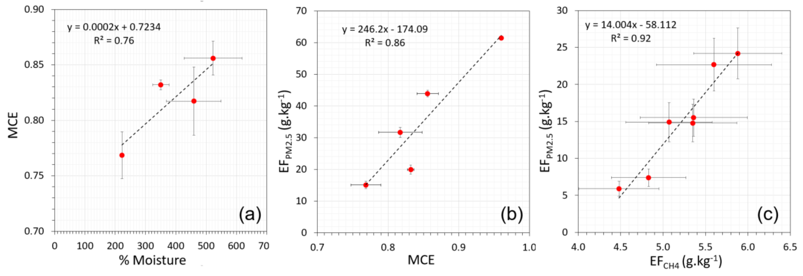
3.1. Peat Physio-Chemical Characteristics

Results from the peat physio-chemical sampling are detailed in Table 2. All peat samples showed a higher C-fraction than most fresh biomass, extending to a maximum of 678 ± 4 g·kg−1 which is typical of histosols having little or no mineral admixtures [63]. Since the sampled smoke came from peat burning occurring at variable depths, the mean (± 1 σ) peat C-content (610 ± 47 g-C·kg−1) was used in the carbon mass balance of Equation (2), and this measured figure is 10.9% higher than the 550 ± 55 g-C·kg−1 assumed by [12], and 5.4% higher than the 579 ± 25 g·kg−1 assumed by [39] during their respective peat fire smoke emissions factor derivations.
Peat substrates all showed high C:N ratios (23 to 56) typical of ombrotrophic peats, while only Location 2 retained a peat O-horizon. This topmost layer showed particularly substantial amounts of partly decayed and strongly rooted organic matter, along with a reduced C:N ratio (20 ± 1) compared to the substrate. This latter feature likely reflects the presence of biotic (i.e., living roots) and/or abiotic (i.e., fertilization) nitrogen enrichment in this surface layer. The peat spectral analyses (see Supplement) confirmed physio-chemical characteristics that varied somewhat with depth as well as location, a finding extending to the moisture content which was substantially lower for the O-horizon than the substrate (see Table 2).

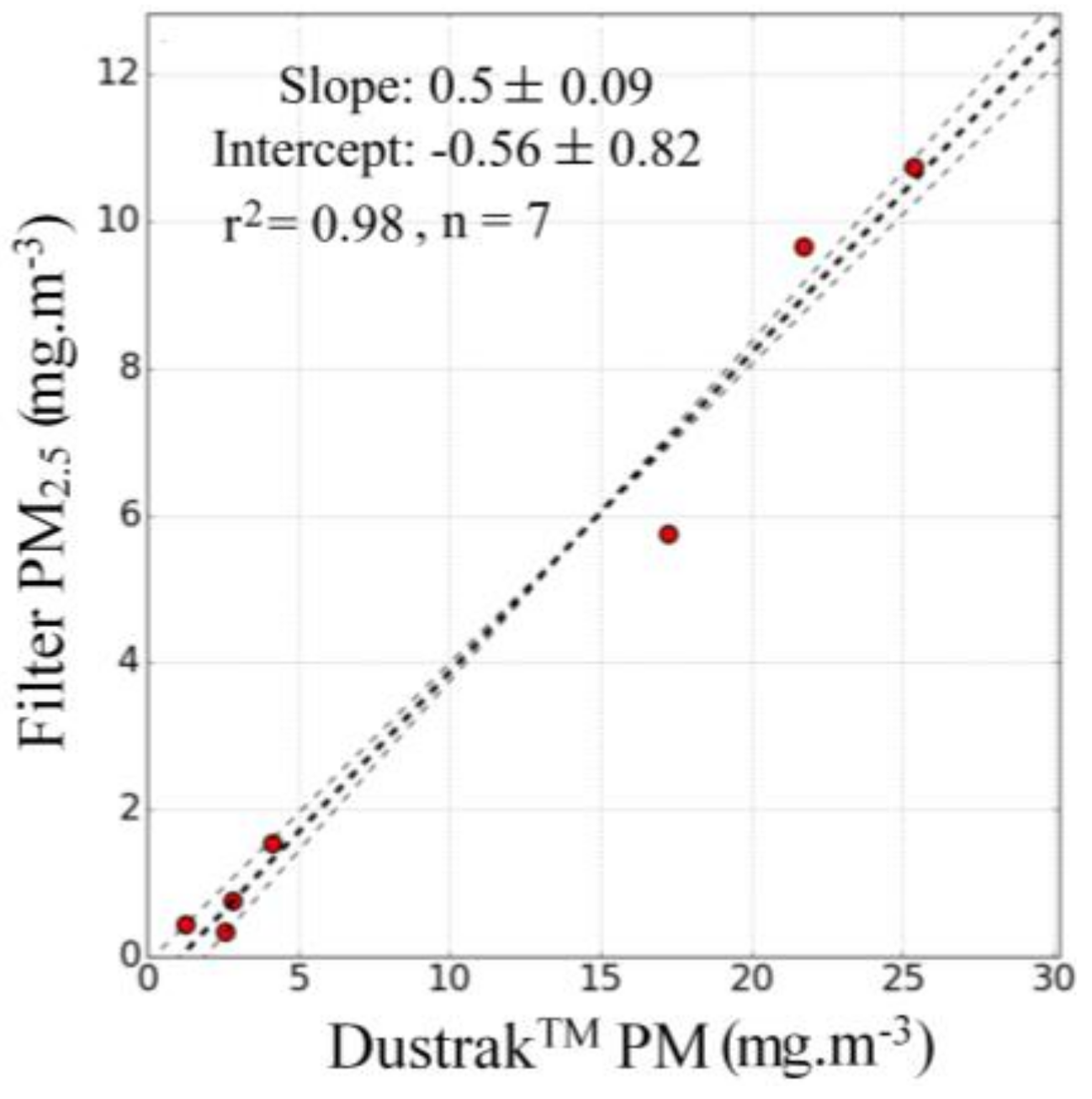
3.2. Calibration of the DustTrak™ PM2.5 Measures

To derive the DustTrak™ peat smoke PM2.5 recalibration factor, the exposed 25 mm Emfab filters were subject to 48 h of post-fire conditioning (matching pre-exposure conditioning at 45–50% RH and 19–21 °C; CEN, 2014). They were then re-weighed using a Mettler-Toledo Ltd. (Leicester, UK) UMX2 balance (0.1 μg resolution) and RMA regression used to compare the DustTrak™ and filter-derived PM2.5 concentrations, this being more appropriate than standard OLS regression when the independent variable also contains uncertainty [64].
Figure 6 shows the derived DustTrak™ re-calibration factor of 0.5 ± 0.09 mg·m−3·(mg·m−3)−1, which is the first for tropical peat fire smoke. This is higher than the 0.37 calculated by [65] for wood smoke, but well within the 0.45 to 0.7 range derived by [48] for a variety of “real-world” biomass burning smoke scenarios.

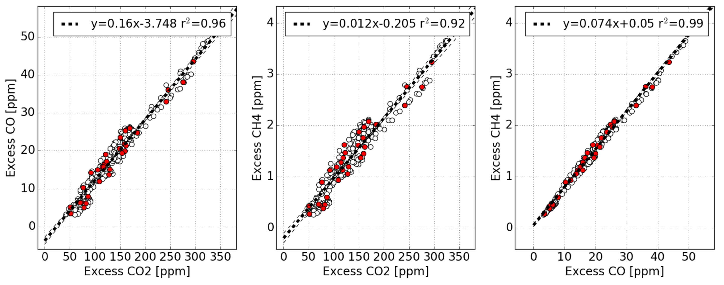
3.3. Trace Gas and Particulate Emissions Ratios

Final per-plume trace gas and particulate ER’s based on the plume integrated analysis approach are listed in Table 3, with the strength of the r2 coefficient of determination used to confirm each ER as well determined [52,66], this exceeding 0.78 and usually 0.90 for all plumes (see example in Figure 5). Figure 7 shows the strong agreement between the locational mean of the plume-integrated ERs and the ER values derived for each of the same locations using the alternative approach of [57] (see Section 2.2.1). The strong, unbiased relationship between the results of the two approaches allays fears of any strong sensitivity to how the timeseries concentration measures were divided into individual plumes during application of the plume integrated analysis method. Table 3 indicates ERs typically varying more between locations than between the plumes of any specific location, particularly with respect to particulate ER’s which show an almost ×20 variation in ERPM2.5/CO between Location 4 (flaming dominated fire in scrubland vegetation atop peat) and Location 5 (pure smoldering sub-surface peat burning).
For the gaseous ERs, Locations 1 and 2 (sites of sub-surface peat burning with very occasional surface vegetation combustion; Table 1) show similar mean ERCO/CO2 values, and their relatively low MCE indicate smoldering-dominated combustion processes. The higher MCE from location 3 indicates a probably greater contribution from flaming combustion, and here the smoke came from burning forest vegetation as well as combusting peat (see Figure 4). Location 4, site of burning scrubland vegetation atop of peat, shows the highest MCE and a likely strong flaming combustion source, whereas location 5 (smoke from sub-surface smoldering peat only) has by far the lowest MCE of any site sampled. For methane, a different emission ratio picture emerges with respect to CO2 than to CO. ERCH4/CO2 for Locations 1 to 3 are quite similar (0.0013 to 0.0015 mol·mol−1), as are those of Locations 4 and 5 (0.00080 to 0.00084 mol·mol−1), despite different fuel mixtures and styles of combustion. ERCH4/CO shows stronger variability however, with plumes at smoldering-dominated Location 5 showing a mean carbon monoxide to methane emission ratio approximately one third of that seen at flaming-dominated Location 4. Locations 1 and 2 also show substantially different ERCH4/CO, despite their similar MCEs and combustion styles. Recent work [67] has highlighted the variability of the emissions ratios characteristic of tropical peatland burning, and our data attest to this variability.

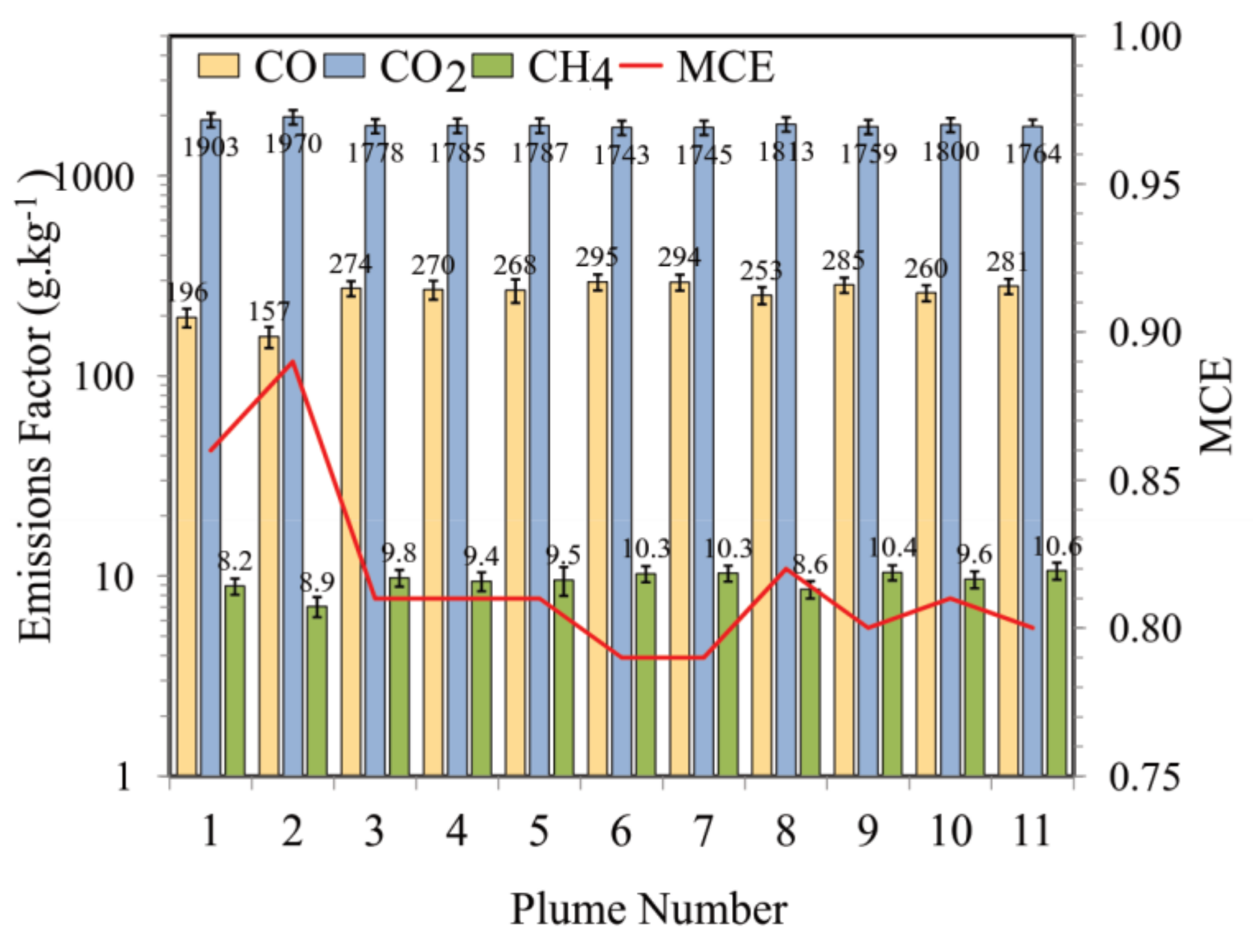
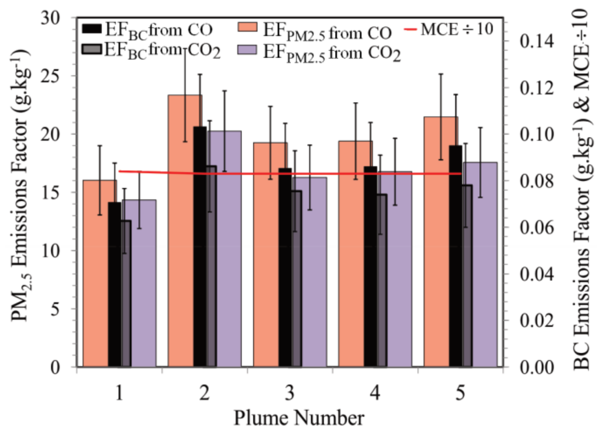
3.4. Trace Gas and Particulate Emissions Factors

Figure 8 graphs exemplar trace gas emissions factors for the Location 1 plumes, and Table 4 presents all EFs derived from all point-based sampling conducted at the fixed measurement locations. Generally, these EF’s agree with those from the OP-FTIR measurements of smoke from the wider combustion zone (also shown in Table 4), confirming the general veracity and representativeness of the point-based measurements. We focus on the point-based data for our detailed analysis, because it is for these that we can definitively identify the source of the smoke being sampled in any particular plume. Huijnen et al. (2012) [12] reported gaseous EFs for a subset of the locations used herein, but even without the further plume measurements included in the current work, our peat carbon content measurements increase the trace gas EFs reported by [12] by more than 10% due to the significantly higher peat carbon fraction we found (Table 2) than was assumed therein.
We confirm high CO emissions factors (and MCE values) at all our sampled locations (bar apparently flaming-dominated Location 4), and this confirms the dominance of smoldering combustion sources at these peatland fires. However, some significant EF variations are seen. For example, the first two plumes sampled at Location 1 show lower EFCO and EFCH4 (and higher MCE) than subsequent plumes, due to more persistent residual (dead) surface vegetation combustion occurring at this time (Figure 8). EFCH4 is rather consistent between Locations 1 and 2 (mean of 9.3 g·kg−1), but at the lowest MCE location (Location 5) it is significantly lower (mean of 5.2 g·kg−1) and counteracted by a higher EFCO (324 g·kg−1 compared to 256 g·kg−1).
Compared to the laboratory-based Indonesian peat burning EFs of [16], who report EFCH4 as 20.8 g·kg−1 (and EFCO as 210 g·kg−1), our in situ derived EFs from the peat-only fires of Locations 1, 2, and 5 (Table 4) are typically significantly lower (higher), though EFCO2 is similar. Laboratory EFs from Indonesian peat burning reported by [37] are more similar to our in situ EFs (they report emissions factors of 12.8 g·kg−1 and 233 g·kg−1 for CH4 and CO respectively), though with some higher EFCH4 values still seen in these laboratory peat fire data. The field-measured EF’s of [39] (based on closed-path FTIR sampling of downwind peat fire smoke) delivered an EFCO of 291 ± 49 g·kg−1 and EFCH4 of 9.5 ± 4.7 g·kg−1, overlapping with our very close-to-source measurements (albeit with higher means). For CO2, [39] provides an EF of 1564 ± 77 g·kg−1, which is low compared to our mean of 1775 g·kg−1 recorded at peat-only fires, but the value from [39] increases by a minimum of 5.4% to 1648 ± 81 g·kg−1 if the peat carbon content assumed in that work (579 ± 25 g·kg−1) is replaced by our higher mean of 610 ± 47 g-C·kg−1 assessed at the actual 2015 fire locations (Section 3.1).
For particulate EFs, Figure 9 shows exemplar values for the five plumes sampled at Location 2. These show almost constant MCE, EFBC and EFPM2.5, with the latter similar whether CO or CO2 is used as the reference gas (see Equation (3) and (4)). Lab-measured EFs of 6.02 g·kg−1 for organic carbon particulates from burning of Indonesian tropical peat were reported by [16], which seem very low compared to our in situ values, while [39] report field EFPM2.5 of 21 ± 4.6 g·kg−1, pleasantly similar to our in situ mean of 17.8 to 22.3 g·kg−1 for peat-only smoke, despite being based on a completely different approach to our DustTrakTM method (specifically photoacoustic extinctiometry, supplemented—as with our approach—by gravimetric filter samples). At Locations 3 and 4 we sampled smoke further downwind from the source, and from fires having an apparently greater flaming contribution (according to the MCE values and landcovers, which included significant vegetation atop the peat). Here we sampled smoke from a combination of peat burning and overlying vegetation combustion, and found EFPM2.5 elevated to 44–61 g·kg−1, very significantly higher than at the locations of sub-surface “pure” peat combustion alone (Locations 1, 2 and 5). This EF is also higher than the pure tropical forest burning EFPM2.5 of 17.8 ± 4 g·kg−1 reported by [68], and the 9.1 ± 3.5 g·kg−1 reported by [54]. Our in situ EFPM2.5 measures recorded at these mixed combustion sites are in fact some of the highest seen for landscape burning, approaching the maximum values reported for some US organic soil burns [69]. Smoke from Locations 3 and 4 also showed a higher black carbon fraction than the peat-only fires, which is in agreement with their partly flaming sourced smoke, though our data overall fully agree with [39] in that organic aerosol (OA) represents the clear majority of PM2.5 from tropical peatland burns (a minimum of 97% in our fires, see Table 3).
Our comparisons between the peat physio-chemical properties (Table 2) and smoke characteristics (Table 4) found only a few noteworthy relationships, most significantly between site-averaged MCE and peat moisture at 10–30 cm depth (Figure 10a), and between site-averaged EFPM2.5 and MCE (Figure 10b). In the latter case, as smoke becomes more dominated by flaming combustion one might normally expect both MCE and EFPM2.5 to decrease. However, we find our two highest EFPM2.5 measures (Table 3) to be from Locations 3 and 4, where we sampled smoke from areas of vegetation combustion atop burning peat (Table 1), and our highest MCEs were also found here—denoting a significant flaming contribution to the emissions. The elevated EFPM2.5 compared to the pure subsurface peat fires may be due to either a change in the combustion characteristics at these mixed combustion sites compared to the pure sub-surface peat burning, or possibly to the impact of nucleation and condensation processes in the (primarily organic aerosol) plume as it is travels from the source to the sampling location (which was more distant for Locations 3 and 4 compared to the very close-to-source sampling possible at Locations 1, 2 and 5). However, in one of a relatively few studies to analyze apparent changes in smoke organic aerosol (OA) emissions factors as plumes age, [56] report that that dilution-driven evaporation of volatile organic compounds dominates over the chemical production of secondary organic aerosol (SOA) within the aging biomass burning plumes sampled, resulting in OA emissions factors that decrease (rather than increase) with time since emission. Furthermore, even at our downwind sampling sites (Locations 3 and 4) our sampling time since emission was far shorter than the many hours investigated by [56] since the sources were hundreds of meters to a few km away, giving relatively limited scope for plume processing to occur.
At single locations where MCE varied significantly between plumes, there were reasonably significant linear relationships between MCE and certain gaseous EFs (up to r2 = 0.82 for EFCH4), as might be expected from past laboratory studies of fire emissions [16]. However, this did not extend to particulate EFs, where the strongest relation was found between EFPM2.5 and EFCH4 at Location 5 (Figure 10c), suggesting a potentially common control on both at this location.

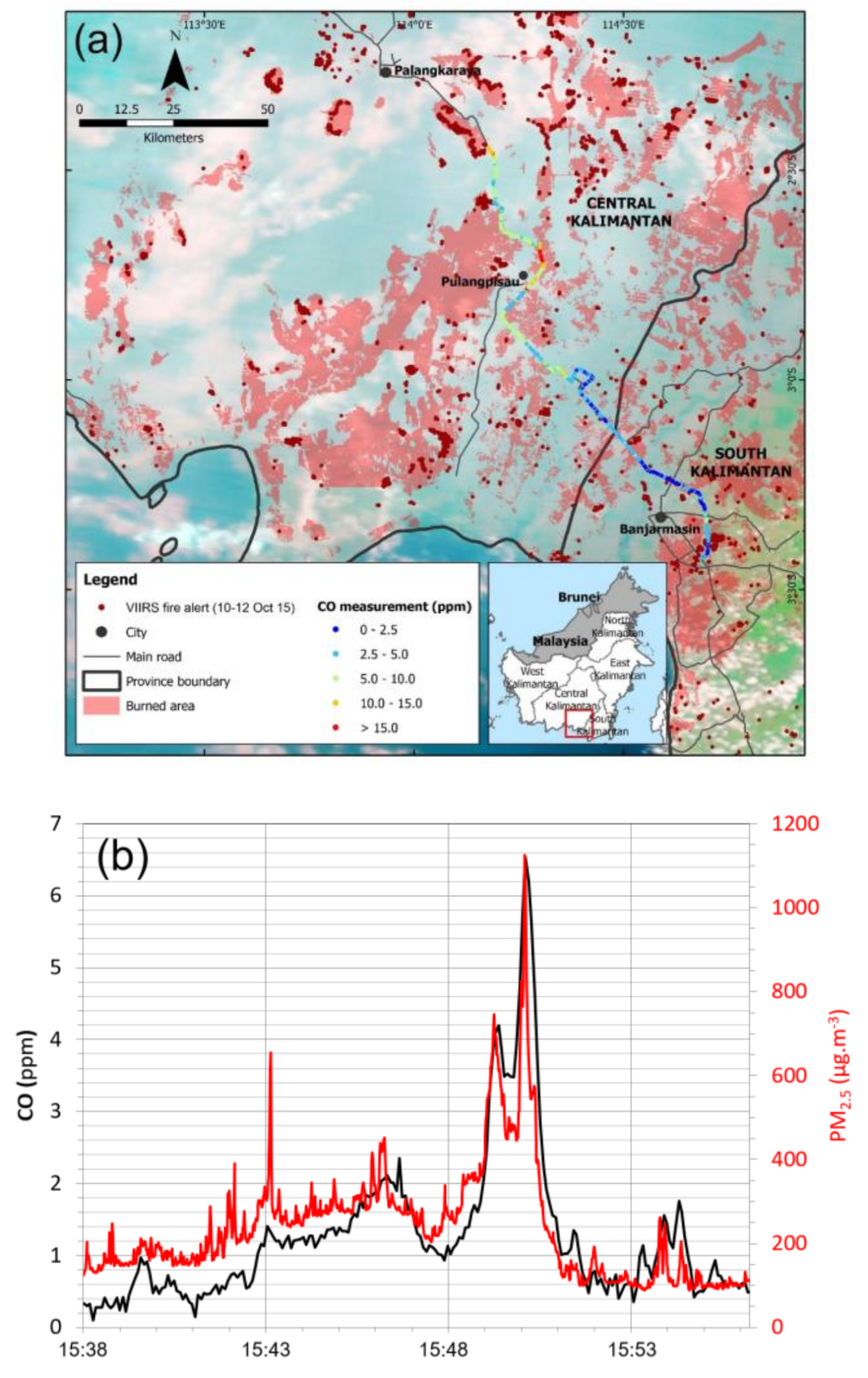
3.5. Transect Measurement Results

CO concentrations sampled on 11 October 2015 along the 240 km long transect moving northwards from the southern coast of Kalimantan (Banjarmasin) are shown in Figure 11a, superimposed on remotely sensed imagery showing the general distribution of haze from MODIS, along with the location of active fires and burned area derived, respectively, using VIIRS [70] and Landsat [36] based methods and satellite data of that same day. Though even the coastal city of Banjarmasin appears to lie just within the haze-affected area according to the background MODIS image, far worse air pollution was found further north, with very significantly elevated carbon monoxide concentrations encountered from around 60 km southeast of Pulangpisau (town marked on Figure 11a). Further north along the road towards Palangkaraya the largest active fire cluster detected by VIIRS can be seen as an extended linear front, located just southwest of the main road and at the border of the final burn scar depicted via the Landsat processing. This is the same fire seen burning in a similar location in the Landsat imagery of 14 October (Figure 3b), located southeast of Palangkaraya in forest vegetation atop peat and indicating the persistence of these peatland fires. Emissions from road traffic prevented detailed analysis of CO2 data recorded during the transect, but CO and CH4 measures showed maxima of 35 ppm and 3.6 ppm respectively during passages through major fire plumes encountered during the 9-h drive. Palangkaraya itself showed CO concentrations of 29.5 ppm in the city center, which whilst not nearly as concerning for health as the ~1000 µg·m−3 of PM10 simultaneously recorded (Figure 11b) this does approach the 1-h CO threshold set for ambient air quality in the region [71], and far exceeds the 8-h mean exposure threshold of 9 ppm. ERCH4/CO encountered on the transect ranged between 0.05 and 0.1 ppmv·ppmv−1, similar to the range recorded at our fixed measurement locations (c.f. location specific ERs reported in Table 3). ERPM2.5/CO recorded during vehicular plume transects also showed values within the range found at our fixed measurement locations reported in Table 3 (e.g., Figure 11b; 0.162 mg·mg−1).

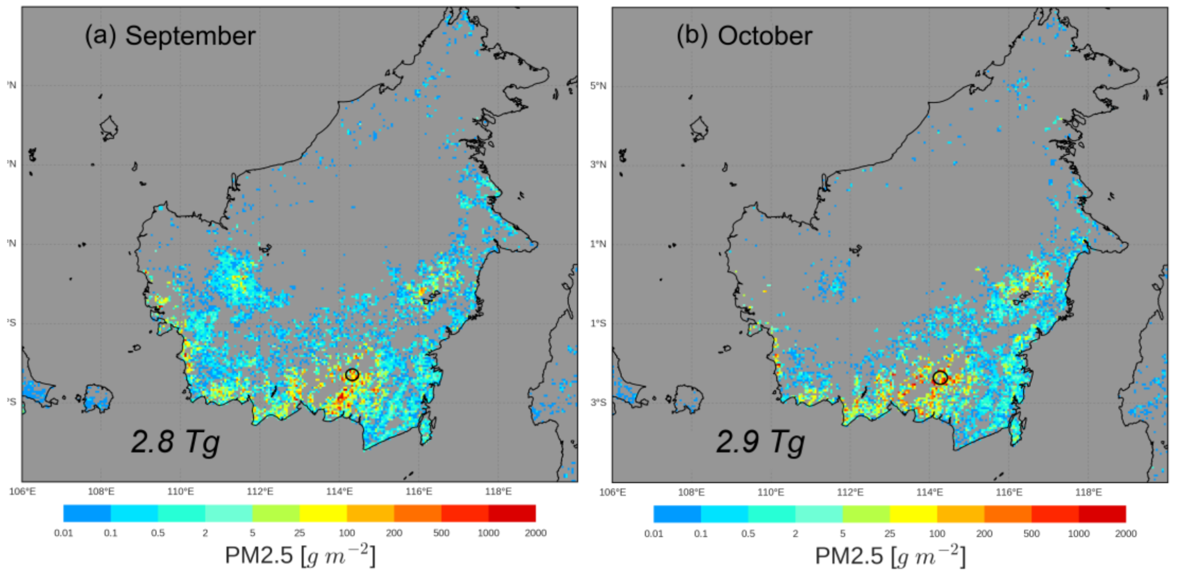
4. New Large-Scale Emissions Estimates

4.1. Peatland EF’s, Gaseous Emissions Totals and Dry Matter Fuel Consumption

In situ gaseous EFs for a subset of the locations included in Table 1 were already reported by [12], upon which the first published total carbonaceous gas emissions calculations for the 2015 Indonesian fire event were based (see [12] for details). The gaseous EFs we report in Table 4 are not only more extensive however, but also greater because they are based on our higher measured peat fractional carbon content (Table 2) rather than the lower C-fraction assumed by [12] whilst measured C-contents were unavailable. Use of our new Table 2 trace gas emissions factors for burning of both pure peat (Locations 1, 2 and 5) and vegetation atop peat (Locations 3 and 4) enables us to calculate “peatland landscape” EFs, based on a 73% weighting of pure peat burning and 27% vegetation burning atop peat following [12,54,72]. These peatland EFs are 1779 ± 55 g·kg−1 for CO2, 238 ± 36 g·kg−1 for CO, and 7.8 ± 2.3 g·kg−1 for CH4, and since they are within 10% of those calculated by [12] using the same weighting factors they provide little evidence for a major change to the total emissions of these three dominant carbonaceous gases reported therein. In fact, to derive total emissions of CO, CO2 and CH4, [12] used a top-down optimization approach based on comparisons between spaceborne MOPITT atmospheric CO concentrations and a priori Global Fire Assimilation System [GFAS] CO emissions from [33] placed within the C-IFS atmospheric chemistry transport model (operated as part of the Copernicus Atmosphere Monitoring Service). The resulting CO emissions estimate reported by [12] is therefore insensitive to changes in EFCO. Furthermore, since the CO2 and CH4 emissions estimates of [12] are based on this top-down, “optimized” CO emissions estimate, along with the ratios of the CO2 and CH4 emissions factors relative to those of CO (rather than the absolute EF values, as would be the case in “bottom-up” calculations such as employed by GFAS [33] and the Global Fire Emissions Database (GFED) [34]), the total CO2 and CH4 emissions estimates provided by [12] are also unaltered by our use of a higher peat carbon content in Equation (2). Table 5 presents the gaseous carbonaceous emissions totals derived by [12] and confirmed herein, and compares these to those reported by GFASv1.2 [33] and GFEDv4.1s [34]. The primary difference is the much larger methane emission total reported by these latter databases, primarily related to their sensitivity to assumed CH4 emissions factors and their assumption of tropical peat and tropical peatland EFCH4 values of 20.8 g·kg−1 and 11.8 g·kg−1 respectively, based primarily on laboratory peat burning and EF summary databases [16,54]. These are far higher than the 7.9 and 7.8 g·kg−1 EFCH4 means we respectively report for ‘pure peat’ and ‘peatland’ fires on the basis of our in situ smoke sampling (Table 4).
To provide the dry matter (DM) fuel consumption estimates for the 2015 Indonesian fires, [12] use their total CO2 emissions estimate (reported in Table 5) and their CO2 emissions factor (use of CO2 is preferred because it is the species whose EF is typically the most consistent between periods of flaming and smoldering and between combustion of different fuel types, as well as it being the species emitted in greatest quantity). Unlike the gaseous emissions estimates, the DM fuel consumption estimate reported by [12] is sensitive to changes in EFCO2, and based on our in situ emissions factor update for these tropical peat and vegetation fires we calculate a new total DM fuel consumption of 358 Tg for Kalimantan and Sumatra during September–October 2015, distributed as shown in Table 6 (we retain the GFASv1.2 standard tropical forest EFCO2 for non-peatland regions of these islands, as did [12]). Our DM fuel consumption total is overall slightly lower than that of [12], reflecting our higher peatland fire CO2 emissions factor (1779 ± 55 g·kg−1) and the fact that the clear majority of the fuel consumption occurred in peatland landscapes. Our DM total is more significantly lower than those of GFEDv4.1s and GFASv1.2 (Table 6), though in fact our Kalimantan total is quite similar to the basic GFAS inventory in September and October, but for Sumatra we calculate greatly reduced values compared to GFAS (primarily because optimization against MOPITT CO significantly lowers the Sumatra emissions compared to the a priori GFAS, as detailed in [12]). GFED’s total DM fuel consumption estimate (461 Tg) is almost exactly midway between that of GFASv1.2 (541 Tg) and the 358 Tg provided by our calculations, but its distribution between islands and between the two months of extreme burning is very different, possibly reflecting major differences between its purely bottom-up methodology and the MODIS burned area product that drives it, and that of the MODIS fire radiative power (FRP)-based GFAS (though the FRP-to-DM conversion factors used by GFAS are based on previous GFAS comparisons to GFED [33]). Overall, our use of MOPITT CO observations, in situ gaseous EFs, and the deployment of these in adjusting the basic GFAS emissions (as detailed in [12] and updated herein) has significantly reduced the DM fuel consumption estimates of the September–October Indonesian fires compared to the most widely used global fire emissions inventories.
Both GFAS and GFED use a PM2.5 emissions factor of 9.1 g·kg−1 for both tropical peatlands and forests, largely based on the EF data included in [54]. This is far lower than every PM2.5 emissions factor derived herein based on in situ measurements of peatland fire smoke (see Table 4), apart from a few plumes encountered at location 5. The most recent GFASv1.2 (0.1° resolution) and GFEDv4.1s (0.25° resolution) show similar September–October 2015 combined Kalimantan and Sumatra fine particulate matter (PM2.5) emissions totals, 3.99 Tg and 4.2 Tg respectively (see Figures S2 and S3), but they also show significant differences in the partitioning between the two months and between the two islands of Kalimantan and Sumatra. This in part reflects the DM fuel consumption differences between these inventories discussed in Section 4.1. Our far higher in situ derived EFPM2.5 values (Section 3.4), along with our updated DM fuel consumptions (Table 6), enables us to provide new PM2.5 emissions totals, and in addition we can utilize the very high temporal resolution (10-min) fire radiative power (FRP) data recently available from the Himawari geostationary satellite [40] to fully resolve the diurnal cycle of these smoke emissions, which can be important when linking them to atmospheric chemistry transport models (CTMs) [71]. Using the data of Table 4, we derive a mean peatland EFPM2.5 of 28 ± 6 g·kg−1, calculated as with the carbonaceous gas EFs from a 73% weighting of pure peat burning and 27% vegetation burning atop peat following [12,54,72]. For non-peatlands we continue use of the 9.1 ± 3.5 g·kg−1 assumed by GFAS and GFED, following [54]. Assuming these emissions factors, our final PM2.5 emissions total for the September–October 2015 Indonesian fires is 9.1 ± 3.2 Tg, two thirds from Kalimantan (Figure 12a,b) and 95% from burning peatlands. We note that some non-peatland fires were in cleared (non-forest) areas, and since [54] assume EFPM2.5 of 15 ± 7 g·kg−1 for “land maintenance fires” these may have a higher EFPM2.5 than pure tropical forest burns. However, substitution of this EF in place of 9.1 ± 3.5 g·kg−1 would elevate our total PM emissions insignificantly, since our calculations indicate that 95% of the PM2.5 emissions come from burning peatlands.
Himawari FRP data [40] enable the spatio-temporal mapping of the particulate emissions at far higher detail than hitherto possible, and whereas their broad spatial pattern (Figure 12a,b) is similar to that reported by GFASv1.2 (Figure A1) and GFEDv4.1s (Figure A2), our 9.1 ± 3.2 Tg PM2.5 emission total is more than double (~×2.2) of those inventories. Their lower totals are primarily driven by their assumed EFPM2.5 of 9.1 g·kg−1, irrespective of whether a fire is burning atop peat, which more than counteracts the fact that both GFASv1.2 and GFEDv4.1s estimate DM fuel consumptions for the 2015 Indonesian fire event to be significantly higher than the 358 Tg upon which our 9.1 ± 3.2 Tg PM2.5 emissions estimate is based (see Table 6). Retaining instead the GFASv1.2 and GFEDv4.1s DM totals from Table 6, but using our updated PM2.5 emissions factors, would increase the magnification of our fine particulate matter emissions estimate over that of the GFED and GFAS values to around ×3. A further global inventory, the Fire Inventory for NCAR (FINN) v2 [73], reports even lower PM emissions than GFEDv4.1s or GFASv1.2, around 5× lower than our 9.1 Tg. Since FINNv2 was recently used as the input for a CTM-based study estimating the extent and severity of short-term health impacts of PM2.5 exposure across Aoutheast Asia (with 6153–17,270 excess mortalities estimated [31]) our significantly higher PM2.5 emissions total suggests a re-appraisal and potential uplift of these impacts maybe necessary. Using a 50% upscaling of the GFASv1.2 PM2.5 emissions, which brings them closer (albeit still well below) those of the current work, [26] previously estimated a much higher excess death total of around 100,000.

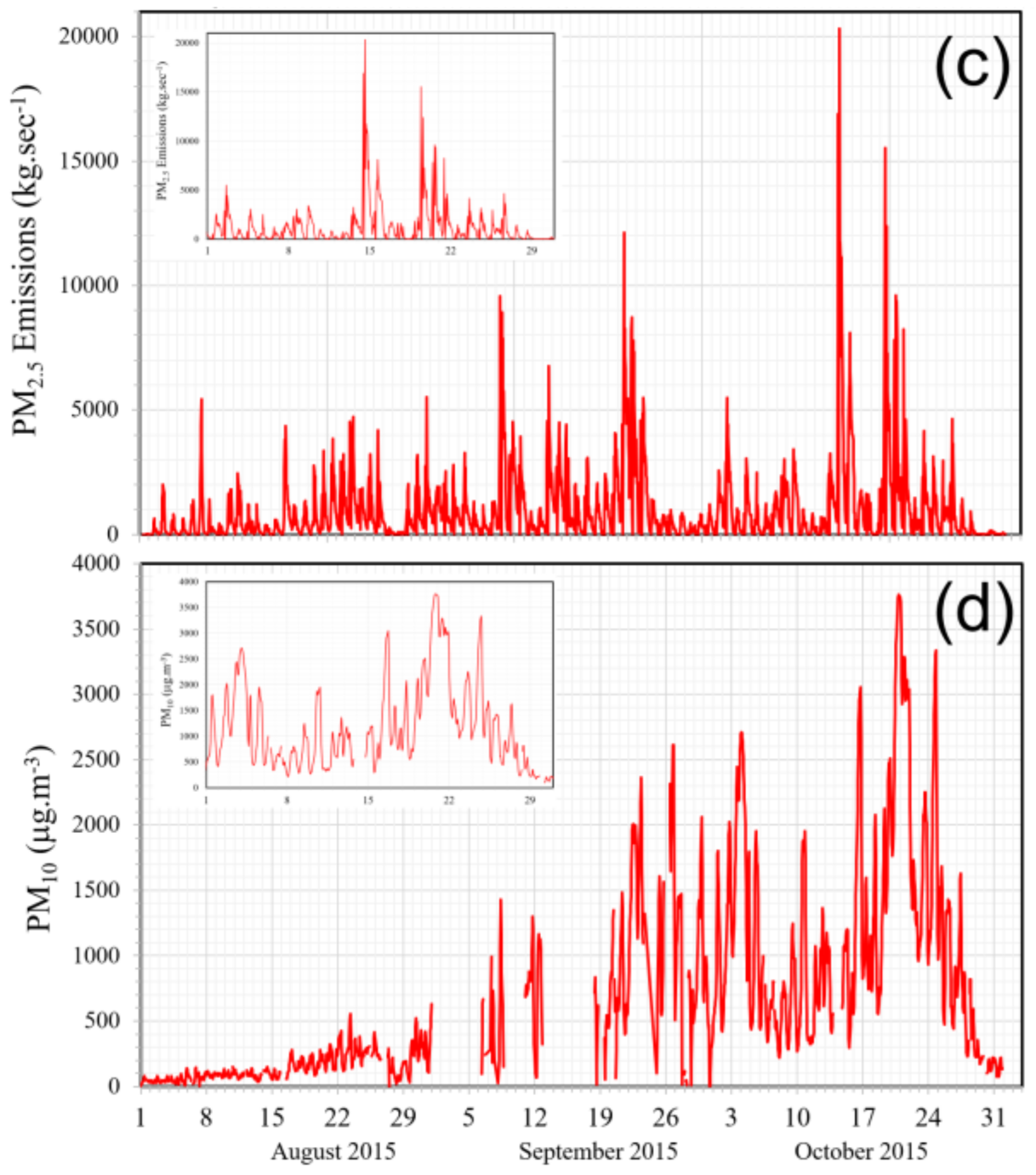
4.2. High Temporal Resolution Emissions

Exploring our very high temporal resolution PM2.5 emissions timeseries (Figure 12c), we see Kalimantans’ smoke particulate emissions rate peaking at more than of 15 tonnes-PM2.5·s−1 in mid-October 2015, shortly before PM10 measurements in Palangkaraya showed their >3000 µg·m−3 concentration maxima (Figure 12d). This maximum is around ten times the threshold considered extremely hazardous for health (see Section 1), and while the daily atmospheric PM concentration cycle recorded at Palangkaraya (Figure 12d) mirrors that seen in the emissions (Figure 12c), they have differently timed peaks because the atmospheric PM concentrations are driven by meteorology, plume processing, and aerosol deposition processes, as well as by the PM emissions rates themselves.
Further investigations using the geostationary FRP-based methodology of [40] indicates that these extreme SE Asian fires show a diurnal cycle peaking generally later in the day than fires dominating most other tropical forest regions, for example those in parts of South America and tropical Africa [74,75,76]. Specifically, the Indonesian fires show a diurnal cycle peaking on average between 16:00 and 18:00 h local solar time (Figure 13), which appears most similar to the peak timing of Brazilian deforestation fires [74] (where fuel is sometimes piled before burning) and fires in the swamp forests of southern Africa [76] (which include areas of tropical peat). The 2015 Indonesian fires also seem to peak significantly later in the day than those seen during more “normal” (non-drought) years in the same region [11,77]. Much of this anomalous fire timing seems likely to be driven by fires in the degraded tropical peatlands accessing the dried-out peat substrate even more significantly during extreme drought than during more “normal” meteorological periods, agreeing with the very significant amplification of Indonesian fire activity often seen during drought events [11,36,42]. Separating out our Himawari-derived 2015 fire diurnal cycles by landcover indicates specifically that Indonesia’s extreme peatland fires (Figure 13a) peak on average ~2 h later in the day than those in non-peat areas burning under the same general climatological conditions (Figure 13b), and the former also show a daily (full width, half-height) fire duration almost twice as long. This may reflect the fact that sub-surface peat combustion, which was seen occurring across very large regions of peatland during our field campaign (e.g., Figure 2b) and which is described in detail in [9], is likely to be less influenced by the daily meteorological cycles of wind, relative humidity and air temperature, factors which (along with ignition timing) typically drive the diurnal variability of surface vegetation fires occurring in non-peat areas [78].

5. Summary and Conclusions

The largest fire events on Earth occur in the deforested and drained tropical peatlands of southeast Asia. Particularly extreme fires develop in these already more flammable degraded landscapes during strong El Niño-related droughts, and the fires on Kalimantan and Sumatra (Indonesia) in September–October 2015 were the greatest such events since the El Niño of 1997–1998 [8,11,12]. The emissions from these fires represent a strong net carbon release to the atmosphere, because their fuel is primarily fossil carbon held in the peat rather than in aboveground vegetation. Furthermore, because peat fires show a strong dominance of smoldering rather than flaming combustion, for the same amount of dry matter burned they tend to emit more carbon monoxide and methane (i.e., have higher CO and CH4 emissions factors), as well as numerous other gaseous air pollutants. Until very recently only laboratory-derived emissions factors were available to support emissions calculations for these globally significant Indonesian peatland fire events, even though their sometimes extreme combustion conditions (e.g., intense forest burning above peat) can be difficult to replicate. Furthermore, while the climatological implications of these massive peatland fires have received a great deal of research attention e.g., [5,7,8], there has been less focus on their human health implications. However, these are likely to be extremely significant [3], especially as (in addition to gaseous air pollutants) small diameter particulate matter (PM10 and PM2.5) is also emitted in more significant quantities during smoldering combustion [20].
Using unique, daily measurements from Indonesia’s air quality monitoring network we have shown that airborne particulate matter concentrations in parts of Indonesia in rose to levels representing some of worst sustained air pollution ever recorded, with maximum reported PM10 exceeding 3800 μg·m−3 in the Capital of Central Kalimantan for example. Independent measurements also show PM2.5 size classes dominating the particulate load, and their smaller diameters mean they are more concerning for human health [79]. Using new in situ measurements of peat physio-chemical properties and smoke plume composition, made at the height and loci of Kalimantan’s most fire affected region, we have derived new carbonaceous trace gas and PM2.5 emissions factors for these peatland fires, sampling a range of combustion conditions from sub-surface “peat only” fires to intense forest fires spreading atop burning peat. Combining these, we derive a peatland fire methane emission factor (7.8 ± 2.3 g·kg−1) very significantly lower than laboratory burns of peat have suggested, and we use this along with our new peatland EFs of CO (238 ± 36 g·kg−1) and CO2 (1779 ± 55 g·kg−1) to confirm earlier estimates made by [12] of the quantities of carbonaceous gases released by the 2015 Indonesian fires, including a methane release (3.2 ± 1.2 Tg) lower by around a factor of three than current global inventories such as GFEDv4.1s, GFASv1.2 and FINNV2 imply. We find tropical peat carbon content at the fire sites to be higher (610 ± 47 g-C·kg−1) than past emissions studies typically assumed, and for some emitted carbonaceous gases this increases our derived EFs over those derived in recent in situ studies, which generally assumed a lower carbon fraction [12,39]. These new data enable us to provide a new dry matter (DM) fuel consumption estimate for the fires on Kalimantan and Sumatra (358 ± 107 Tg, 85% of which is peat), and this is again lower than current global biomass burning inventories imply. Even when maintaining the higher GFED and GFAS fuel consumptions in such calculations, our reduced peatland EFCH4 based on in situ measurements of smoke suggests a total methane release by these fires more than a factor of two lower than these inventories (which use a EFCH4 that is at or close-to the laboratory derived values).
Our peat sampling shows an O-horizon layer exists only at the visited locations on Kalimantan that had not experienced fire since the 1997–1998 El Niño, and this layers layer’s light, aerated structure and significantly lower moisture content compared to the deeper layers appears to indicate a mechanism by which fire may accelerate from the surface vegetation into the peat. Specifically, the more easily ignitable O-horizon seems likely to aid combustion taking hold at the surface before penetrating the underlying, denser, wetter (and more difficult to ignite), but more carbon rich, peat substrate. Once burning we found the peat to emit particulate matter in great quantities. We find PM2.5 emissions factors, based on our field measurements, far higher than those seen in laboratory tropical peat burning. We derive an EFPM2.5 of 22.3 ± 8.7 g·kg−1 for smoldering peat only fires measured very close to source, find even higher PM2.5 emissions factors (44–61 g·kg−1) at sites of vegetation fires atop burning peat, though these latter measurements had to be made further downwind (maximum of a few km) due to safety concerns. These “vegetation and peat fire” PM2.5 emissions factors represent some of the highest seen worldwide, approaching the maxima reported for some US organic soil burns [69]. Smoldering combustion produces PM mainly via condensation of volatilized organics onto existing particles and surfaces [20], helping explain why peatland fires produce emissions deficient in black carbon and whose particulate load is dominated by organic aerosol (OA), and this is the case even in the mixed vegetation and peat fires. Our in situ data indicate that OA makes up a minimum of 97% of the overall emitted PM2.5 mass. We reject significant OA production during the period between the emission and measurement of these downwind-sampled “combined vegetation atop peat” fire plumes, because field experiments have found that (downwind) dilution generally reduces, rather increases, primary OA concentrations [56]. Furthermore, while significant lofting (and thus cooling), of plumes can lead to condensing of gas phase material and thus to PM2.5 concentration increases [80], this was not a feature of the ground-level ‘vegetation and peat fire’ plumes sampled here. Therefore, we conclude that their increased EFPM2.5 compared to the “peat only” fires is because peatland burning incorporating significant surface vegetation combustion can occur in ways that maximizes the emission of fine particulates. We hypothesize that this could be due to (i) the peat being partly consumed in higher temperature flaming combustion driven by the surface vegetation fires, with temperature-related effects on emissions from peat fires already having been noted by [67], and/or (ii) because the spreading vegetation fire atop the peat enables rapid access to new peat fuel that is burnt initially at the surface, and that this may in turn maximize PM2.5 emissions factors by continually generating new areas of surface peat combustion in which particulate release to the atmosphere is far stronger than that in peat-only fires, which typically propagate below the surface layer [9] and which may thus not be in direct contact with the open atmosphere. Combing our pure “sub-surface peat” and “vegetation atop peat” PM2.5 emissions factors, we derive an overall EFPM2.5 for these Indonesian tropical peatland fires of 28 ± 6 g·kg−1, around three times that assumed in current fire emissions inventories such as GFEDv4.1s, GFASv1.2 and FINN [33,34,73].
Using our updated dry matter (DM) fuel consumption and EFPM2.5 measures, we estimate total September and October 2015 PM2.5 emissions for fires on Kalimantan and Sumatra to be 2× to 5.5× higher than those of GFEDv4.1s, GFASv1.2 and FINNv2, and we use geostationary, very high temporal resolution fire radiative power (FRP) data to illustrate for the first time that the fire diurnal cycle in these tropical peatland areas is significantly wider and peaks later in the day than in non-peatland areas subject to the same drought conditions. The long duration, extremely large areas of simultaneous burning, the very high fuel consumptions per unit area, and the very high PM2.5 emissions factors found in these peatlands made these Indonesian fires the greatest wildfire sources of PM2.5 in 2015, and combining our updated PM2.5 emissions factors with data from the long-term GFAS and GFED inventories (which stretch back to the early 2000’s) we find such equatorial southeast Asian fires to be commonly among the top five wildfire PM sources worldwide. Given the conclusion from a recent Mexico City epidemiological study that a 1 µg·m−3 increase in 24-h PM10 exposure led to 0.24 infant deaths per 100,000 births [81], we agree with [25,26,31] that the very high particulate matter emissions and extreme, perhaps almost unprecedented, atmospheric PM loadings seen over parts of Kalimantan and Sumatra throughout much of September and October 2015 as a result of these fires provides a serious cause for concern.

Supplementary Materials

The following are available online at https://www.mdpi.com/2072-4292/10/4/495/s1, Figure S1: Absorbance spectra (350–2500 nm) recorded from dried peat samples collected in three soil layers (Surface, 0–10 cm and 10–30 cm depth). Figure S2: Monthly mean PM2.5 fire emissions per grid cell unit area (kg·m−2) as reported by GFASv1.2 for September and October 2015. Figure S3: Monthly mean PM2.5 fire emissions per 0.25° grid cell unit area (kg·m−2) as reported by GFEDv4.1s for September and October 2015.

Acknowledgments

This study was supported primarily by funding from the Natural Environment Research Council (NERC) of the UK (PR140015 and NE/M017729/1). We thank the anonymous reviewers for their insightful comments and suggestions. The work contains modified Copernicus Atmosphere Monitoring Service Information [2018], and neither the European Commission nor ECMWF is responsible for any use that may be made of the information it contains.

Author Contributions

M.J.W. conceived the study, M.J.W., D.L.A.G., D.M., and D.C.G. designed details of the approach; M.J.W., D.L.A.G., D.M., M.A.S., B.M. and A.S. performed the field measurements; M.J.W., T.Z., and D.G. analyzed the in situ trace gas and particulate data, and D.G. the air quality data; V.H., W.X., T.Z. and M.J.W. analyzed the satellite and fire emissions inventory data, N.B. and M.S. analyzed the peat spectral and physio-chemical data; M.J.W. wrote the paper.

Conflicts of Interest

The authors declare no conflict of interest.

Appendix A

Figure A1. Monthly mean PM2.5 emissions per grid cell unit area (kg·m−2) as reported by GFASv1.2 for September and October 2015 based on MODIS FRP, shown at both the original 0.5° resolution of [33] (top row) and the more recent 0.1° resolution of GFAS (bottom row). Total monthly PM2.5 emissions for Sumatra and Kalimantan are indicated and are very similar for both resolution datasets.
Remotesensing 10 00495 g0a1
Figure A2. Monthly mean PM2.5 emissions per 0.25° grid cell unit area (kg·m−2) as reported by GFEDv4.1s for September and October 2015 and based on MODIS MCD64A1 burned area data and fuel consumption modelling, as detailed in [34]. Monthly PM2.5 emissions for Sumatra and Kalimantan are indicated, which reduce from a total of 4.2 Tg to 3.7 Tg if the effect of the “small fire” boosting used in GFED4.1s is removed.
Remotesensing 10 00495 g0a2

References

  1. Field, R.D.; Werf, G.R.V.D.; Shen, S.S.P. Human amplification of drought-Induced biomass burning in Indonesia since 1960. Nat. Geosci. 2009, 2, 185–188. [Google Scholar] [CrossRef]
  2. Gaveau, D.L.; Pirard, R.; Salim, M.A.; Tonoto, P.; Yaen, H.; Parks, S.A.; Carmenta, R. Overlapping land claims limit the use of satellites to monitor no-deforestation commitments and no-burning compliance. Conserv. Lett. 2016, 10, 257–264. [Google Scholar] [CrossRef]
  3. Aditama, T.Y. Impact of haze from forest fire to respiratory health: Indonesian experience. Respirology 2000, 5, 169–174. [Google Scholar] [CrossRef] [PubMed]
  4. Reisen, F.; Duran, S.M.; Flannigan, M.; Elliott, C.; Rideout, K. Wildfire smoke and public health risk. Int. J. Wildland Fire 2015, 24, 1029–1044. [Google Scholar] [CrossRef]
  5. Keywood, M.; Kanakidou, M.; Stohl, A.; Dentener, F.; Grassi, G.; Meyer, C.P.; Torseth, K.; Edwards, D.; Thompson, A.M.; Lohmann, U.; et al. Fire in the Air: Biomass Burning Impacts in a Changing Climate. Crit. Rev. Environ. Sci. Technol. 2013, 43, 40–83. [Google Scholar] [CrossRef]
  6. Jaenicke, J.; Rieley, J.; Mott, C.; Kimman, P.; Siegert, F. Determination of the amount of carbon stored in Indonesian peatlands. Geoderma 2008, 147, 151–158. [Google Scholar] [CrossRef]
  7. Couwenberg, J.; Dommain, R.; Joosten, H. Greenhouse gas fluxes from tropical peatlands in south-East Asia. Glob. Chang. Biol. 2009, 16, 1715–1732. [Google Scholar] [CrossRef]
  8. Page, S.E.; Rieley, J.O.; Banks, C.J. Global and regional importance of the tropical peatland carbon pool. Glob. Chang. Biol. 2011, 17, 798–818. [Google Scholar] [CrossRef]
  9. Usup, A.; Hashimoto, Y.; Takahashi, H.; Hayasaka, H. Combustion and thermal characteristics of peat fire in tropical peatland in Central Kalimantan, Indonesia. Tropics 2004, 14, 1–19. [Google Scholar] [CrossRef]
  10. Murdiyarso, D.; Adiningsih, E.S. Climate anomalies, Indonesian vegetation fires and terrestrial carbon emissions. Mitig. Adapt. Strateg. Glob. Chang. 2006, 12, 101–112. [Google Scholar] [CrossRef]
  11. Wooster, M.J.; Perry, G.L.W.; Zoumas, A. Fire, drought and El Niño relationships on Borneo (Southeast Asia) in the pre-MODIS era (1980–2000). Biogeosciences 2012, 9, 317–340. [Google Scholar] [CrossRef]
  12. Huijnen, V.; Wooster, M.J.; Kaiser, J.W.; Gaveau, D.L.A.; Flemming, J.; Parrington, M.; Inness, A.; Murdiyarso, D.; Main, B.; Weele, M.V. Fire carbon emissions over maritime southeast Asia in 2015 largest since 1997. Sci. Rep. 2016, 6. [Google Scholar] [CrossRef] [PubMed]
  13. Leeuwen, T.T.V.; Werf, G.R.V.D.; Hoffmann, A.A.; Detmers, R.G.; Rücker, G.; French, N.H.F.; Archibald, S.; Carvalho, J.A.; Cook, G.D.; Groot, W.J.D.; et al. Biomass burning fuel consumption rates: A field measurement database. Biogeosciences 2014, 11, 7305–7329. [Google Scholar] [CrossRef]
  14. Simpson, J.; Wooster, M.; Smith, T.; Trivedi, M.; Vernimmen, R.; Dedi, R.; Shakti, M.; Dinata, Y. Tropical Peatland Burn Depth and Combustion Heterogeneity Assessed Using UAV Photogrammetry and Airborne LiDAR. Remote Sens. 2016, 8, 1000. [Google Scholar] [CrossRef]
  15. Werf, G.R.V.D.; Morton, D.C.; Defries, R.S.; Olivier, J.G.J.; Kasibhatla, P.S.; Jackson, R.B.; Collatz, G.J.; Randerson, J.T. CO2 emissions from forest loss. Nat. Geosci. 2009, 2, 737–738. [Google Scholar] [CrossRef]
  16. Christian, T.J. Comprehensive laboratory measurements of biomass-Burning emissions: 1. Emissions from Indonesian, African, and other fuels. J. Geophys. Res. 2004, 108. [Google Scholar] [CrossRef]
  17. Ward, D.E. Factors Influencing the Emissions of Gases and Particulate Matter from Biomass Burning. Ecol. Stud. Fire Trop. Biota 1990, 84, 418–436. [Google Scholar]
  18. Rein, G. Smouldering Fires and Natural Fuels. In Fire Phenomena and the Earth System; John Wiley and Sons, Ltd.: Chichester, UK, 2013; pp. 15–33. [Google Scholar]
  19. Whitburn, S.; Damme, M.V.; Clarisse, L.; Turquety, S.; Clerbaux, C.; Coheur, P.-F. Doubling of annual ammonia emissions from the peat fires in Indonesia during the 2015 El Niño. Geophys. Res. Lett. 2016, 43, 11007–11014. [Google Scholar] [CrossRef]
  20. Reid, J.S.; Koppmann, R.; Eck, T.F.; Eleuterio, D.P. A review of biomass burning emissions, part II: Intensive physical properties of biomass burning particles. Atmos. Chem. Phys. 2004, 5, 799–825. [Google Scholar] [CrossRef]
  21. Haikerwal, A.; Akram, M.; Monaco, A.D.; Smith, K.; Sim, M.R.; Meyer, M.; Tonkin, A.M.; Abramson, M.J.; Dennekamp, M. Impact of Fine Particulate Matter (PM2.5) exposure during wildfires on cardiovascular health outcomes. J. Am. Heart Assoc. 2015, 4, e001653. [Google Scholar] [CrossRef] [PubMed]
  22. Liu, J.C.; Pereira, G.; Uhl, S.A.; Bravo, M.A.; Bell, M.L. A systematic review of the physical health impacts from non-occupational exposure to wildfire smoke. Environ. Res. 2015, 136, 120–132. [Google Scholar] [CrossRef] [PubMed]
  23. Chisholm, R.A.; Wijedasa, L.S.; Swinfield, T. The need for long-Term remedies for Indonesia’s forest fires. Conserv. Biol. 2016, 30, 5–6. [Google Scholar] [CrossRef] [PubMed]
  24. Adetona, O.; Reinhardt, T.E.; Domitrovich, J.; Broyles, G.; Adetona, A.M.; Kleinman, M.T.; Ottmar, R.D.; Naeher, L.P. Review of the health effects of wildland fire smoke on wildland firefighters and the public. Inhal. Toxicol. 2016, 28, 95–139. [Google Scholar] [CrossRef] [PubMed]
  25. Tacconi, L. Preventing fires and haze in Southeast Asia. Nat. Clim. Chang. 2016, 6, 640. [Google Scholar] [CrossRef]
  26. Koplitz, S.N.; Mickley, L.J.; Marlier, M.E.; Buonocore, J.J.; Kim, P.S.; Liu, T.; Sulprizio, M.P.; Defries, R.S.; Jacob, D.J.; Schwartz, J.; et al. Public health impacts of the severe haze in Equatorial Asia in September–October 2015: Demonstration of a new framework for informing fire management strategies to reduce downwind smoke exposure. Environ. Res. Lett. 2016, 11, 094023. [Google Scholar] [CrossRef]
  27. Betha, R.; Behera, S.N.; Balasubramanian, R. 2013 Southeast Asian smoke haze: Fractionation of particulate-bound elements and associated health risk. Environ. Sci. Technol. 2014, 48, 4327–4335. [Google Scholar] [CrossRef] [PubMed]
  28. Kunii, O.; Kanagawa, S.; Yajima, I.; Hisamatsu, Y.; Yamamura, S.; Amagai, T.; Ismail, I.T.S. The 1997 haze disaster in Indonesia: Its air quality and health effects. Arch. Environ. Health 2002, 57, 16–22. [Google Scholar] [CrossRef] [PubMed]
  29. Marlier, M.E.; Defries, R.S.; Voulgarakis, A.; Kinney, P.L.; Randerson, J.T.; Shindell, D.T.; Chen, Y.; Faluvegi, G. El Niño and health risks from landscape fire emissions in southeast Asia. Nat. Clim. Chang. 2012, 3, 131–136. [Google Scholar] [CrossRef] [PubMed]
  30. Aouizerats, B.; Werf, G.R.V.D.; Balasubramanian, R.; Betha, R. Importance of transboundary transport of biomass burning emissions to regional air quality in Southeast Asia during a high fire event. Atmos. Chem. Phys. 2015, 15, 363–373. [Google Scholar] [CrossRef]
  31. Crippa, P.; Castruccio, S.; Archer-Nicholls, S.; Lebron, G.B.; Kuwata, M.; Thota, A.; Sumin, S.; Butt, E.; Wiedinmyer, C.; Spracklen, D.V. Population exposure to hazardous air quality due to the 2015 fires in Equatorial Asia. Sci. Rep. 2016, 6. [Google Scholar] [CrossRef] [PubMed]
  32. Yorifuji, T.; Bae, S.; Kashima, S.; Tsuda, T.; Doi, H.; Honda, Y.; Kim, H.; Hong, Y.-C. Health Impact Assessment of PM10 and PM2.5 in 27 Southeast and East Asian Cities. J. Occup. Environ. Med. 2015, 57, 751–756. [Google Scholar] [CrossRef] [PubMed]
  33. Kaiser, J.W.; Heil, A.; Andreae, M.O.; Benedetti, A.; Chubarova, N.; Jones, L.; Morcrette, J.-J.; Razinger, M.; Schultz, M.G.; Suttie, M.; et al. Biomass burning emissions estimated with a global fire assimilation system based on observed fire radiative power. Biogeosciences 2012, 9, 527–554. [Google Scholar] [CrossRef] [Green Version]
  34. Van Der Werf, G.R.; Randerson, J.T.; Giglio, L.; Van Leeuwen, T.T.; Chen, Y.; Rogers, B.M.; Mu, M.; Van Marle, M.J.; Morton, D.C.; Collatz, G.J.; et al. Global fire emissions estimates during 1997–2016. Earth Syst. Sci. Data 2017, 9, 697–720. [Google Scholar] [CrossRef]
  35. Mota, B.; Wooster, M.J. A new top-Down approach for directly estimating biomass burning emissions and fuel consumption rates and totals from geostationary satellite fire radiative power (FRP). Remote Sens. Environ. 2018, 206, 45–62. [Google Scholar] [CrossRef]
  36. Gaveau, D.L.A.; Salim, M.A.; Hergoualch, K.; Locatelli, B.; Sloan, S.; Wooster, M.; Marlier, M.E.; Molidena, E.; Yaen, H.; Defries, R.; et al. Major atmospheric emissions from peat fires in Southeast Asia during non-Drought years: Evidence from the 2013 Sumatran fires. Sci. Rep. 2014, 4, 6112. [Google Scholar] [CrossRef] [PubMed] [Green Version]
  37. Stockwell, C.E.; Yokelson, R.J.; Kreidenweis, S.M.; Robinson, A.L.; Demott, P.J.; Sullivan, R.C.; Reardon, J.; Ryan, K.C.; Griffith, D.W.T.; Stevens, L. Trace gas emissions from combustion of peat, crop residue, biofuels, grasses, and other fuels: Configuration and FTIR component of the fourth Fire Lab at Missoula Experiment (FLAME-4). Atmos. Chem. Phys. 2014, 14, 9727–9754. [Google Scholar] [CrossRef]
  38. Delmas, R.; Lacaux, J.P.; Brocard, D. Determination of Biomass Burning Emission Factors: Methods and Results. Environ. Monit. Assess. 1995, 38, 181–204. [Google Scholar] [CrossRef] [PubMed]
  39. Stockwell, C.E.; Jayarathne, T.; Cochrane, M.A.; Ryan, K.C.; Putra, E.I.; Saharjo, B.H.; Nurhayati, A.D.; Albar, I.; Blake, D.R.; Simpson, I.J.; et al. Field measurements of trace gases and aerosols emitted by peat fires in Central Kalimantan, Indonesia during the 2015 El Niño. Atmos. Chem. Phys. 2016, 16, 11711–11732. [Google Scholar] [CrossRef]
  40. Xu, W.; Wooster, M.J.; Kaneko, T.; He, J.; Zhang, T.; Fisher, D. Major advances in geostationary fire radiative power (FRP) retrieval over Asia and Australia stemming from use of Himarawi-8 AHI. Remote Sens. Environ. 2017, 193, 138–149. [Google Scholar] [CrossRef]
  41. Blake, D.; Hinwood, A.; Horwitz, P. Peat fires and air quality: Volatile organic compounds and particulates. Chemosphere 2009, 76, 419–423. [Google Scholar] [CrossRef] [PubMed]
  42. Field, R.D.; Werf, G.R.V.D.; Fanin, T.; Fetzer, E.J.; Fuller, R.; Jethva, H.; Levy, R.; Livesey, N.J.; Luo, M.; Torres, O.; et al. Indonesian fire activity and smoke pollution in 2015 show persistent nonlinear sensitivity to El Niño-Induced drought. Proc. Natl. Acad. Sci. USA 2016, 113, 9204–9209. [Google Scholar] [CrossRef] [PubMed]
  43. Emmanuel, S.C. Impact to lung health of haze from forest fires: The Singapore experience. Respirology 2000, 5, 175–182. [Google Scholar] [CrossRef] [PubMed]
  44. Statheropoulos, M.; Karma, S. Complexity and origin of the smoke components as measured near the flame-Front of a real forest fire incident: A case study. J. Anal. Appl. Pyrolysis 2007, 78, 430–437. [Google Scholar] [CrossRef]
  45. Zhang, T.; Wooster, M.J.; Green, D.C.; Main, B. New field-Based agricultural biomass burning trace gas, PM 2.5, and black carbon emission ratios and factors measured in situ at crop residue fires in Eastern China. Atmos. Environ. 2015, 121, 22–34. [Google Scholar] [CrossRef]
  46. Cheng, Y.-H. Real-Time Performance of the microAeth® AE51 and the Effects of Aerosol Loading on Its Measurement Results at a Traffic Site. Aerosol Air Qual. Res. 2013, 13, 1853–1863. [Google Scholar] [CrossRef]
  47. Nussbaum, N.J.; Zhu, D.; Kuhns, H.D.; Mazzoleni, C.; Chang, M.-C.O.; Moosmüller, H.; Watson, J.G. The in-plume emission test stand: An instrument platform for the real-time characterization of fuel-based combustion emissions. J. Air Waste Manag. Assoc. 2009, 59, 1437–1445. [Google Scholar] [CrossRef] [PubMed]
  48. McNamara, M.L. Correction Factor for Continuous Monitoring of Wood Smoke Fine Particulate Matter. Aerosol Air Qual. Res. 2011, 11, 315. [Google Scholar] [CrossRef] [PubMed]
  49. Yokelson, R.J.; Griffith, D.W.; Ward, D.E. Open-path Fourier transform infrared studies of large-scale laboratory biomass fires. J. Geophys. Res. Atmos. 1996, 101, 21067–21080. [Google Scholar] [CrossRef]
  50. Oshea, S.J.; Bauguitte, S.J.-B.; Gallagher, M.W.; Lowry, D.; Percival, C.J. Development of a cavity-Enhanced absorption spectrometer for airborne measurements of CH4 and CO2. Atmos. Meas. Tech. 2013, 6, 1095–1109. [Google Scholar] [CrossRef]
  51. Roberts, T.; Saffell, J.; Oppenheimer, C.; Lurton, T. Electrochemical sensors applied to pollution monitoring: Measurement error and gas ratio bias—A volcano plume case study. J. Volcanol. Geotherm. Res. 2014, 281, 85–96. [Google Scholar] [CrossRef]
  52. Wooster, M.J.; Freeborn, P.H.; Archibald, S.; Oppenheimer, C.; Roberts, G.J.; Smith, T.E.L.; Govender, N.; Burton, M.; Palumbo, I. Field determination of biomass burning emission ratios and factors via open-Path FTIR spectroscopy and fire radiative power assessment: Headfire, backfire and residual smouldering combustion in African savannahs. Atmos. Chem. Phys. 2011, 11, 11591–11615. [Google Scholar] [CrossRef] [Green Version]
  53. Yokelson, R.J.; Goode, J.G.; Ward, D.E.; Susott, R.A.; Babbitt, R.E.; Wade, D.D.; Bertschi, I.; Griffith, D.W.T.; Hao, W.M. Emissions of formaldehyde, acetic acid, methanol, and other trace gases from biomass fires in North Carolina measured by airborne Fourier transform infrared spectroscopy. J. Geophys. Res. Atmos. 1999, 104, 30109–30125. [Google Scholar] [CrossRef]
  54. Akagi, S.K.; Yokelson, R.J.; Wiedinmyer, C.; Alvarado, M.J.; Reid, J.S.; Karl, T.; Crounse, J.D.; Wennberg, P.O. Emission factors for open and domestic biomass burning for use in atmospheric models. Atmos. Chem. Phys. Discuss. 2010, 11, 4039–4072. [Google Scholar] [CrossRef]
  55. Goode, J.G.; Yokelson, R.J.; Ward, D.E.; Susott, R.A.; Babbitt, R.E.; Davies, M.A.; Hao, W.M. Measurements of excess O3, CO2, CO, CH4, C2H4, C2H2, HCN, NO, NH3, HCOOH, CH3COOH, HCHO, and CH3OH in 1997 Alaskan biomass burning plumes by airborne Fourier transform infrared spectroscopy (AFTIR). J. Geophys. Res. Atmos. 2000, 105, 22147–22166. [Google Scholar] [CrossRef]
  56. May, A.A.; Lee, T.; Mcmeeking, G.R.; Akagi, S.; Sullivan, A.P.; Urbanski, S.; Yokelson, R.J.; Kreidenweis, S.M. Observations and analysis of organic aerosol evolution in some prescribed fire smoke plumes. Atmos. Chem. Phys. 2015, 15, 6323–6335. [Google Scholar] [CrossRef]
  57. Bentley, S. Graphical techniques for constraining estimates of aerosol emissions from motor vehicles using air monitoring network data. Atmos. Environ. 2004, 38, 1491–1500. [Google Scholar] [CrossRef]
  58. Grange, S.K.; Lewis, A.C.; Carslaw, D.C. Source apportionment advances using polar plots of bivariate correlation and regression statistics. Atmos. Environ. 2016, 145, 128–134. [Google Scholar] [CrossRef]
  59. Ayers, G. Comment on regression analysis of air quality data. Atmos. Environ. 2001, 35, 2423–2425. [Google Scholar] [CrossRef]
  60. Hagler, G.S. Post-processing method to reduce noise while preserving high time resolution in aethalometer real-time black carbon data. Aerosol Air Qual. Res. 2011, 11, 539–546. [Google Scholar] [CrossRef]
  61. Balasubramanian, R. Comprehensive characterization of PM2.5 aerosols in Singapore. J. Geophys. Res. 2004, 108, 2022–2156. [Google Scholar]
  62. Briz, S.; Castro, A.J.D.; Díez, S.; López, F.; Schäfer, K. Remote sensing by open-Path FTIR spectroscopy. Comparison of different analysis techniques applied to ozone and carbon monoxide detection. J. Quant. Spectrosc. Radiat. Transf. 2007, 103, 314–330. [Google Scholar] [CrossRef]
  63. Osaki, M.; Hirose, K.; Segah, H.; Helmy, F. Tropical Peat and Peatland Definition in Indonesia. Trop. Peatl. Ecosyst. 2016, 137–147. [Google Scholar]
  64. Sokal, R.R.; James, R.F. The Principles and Practice of Statistics in Biological Research, 3rd ed.; W.H. Freeman and Company: New York, NY, USA, 1995. [Google Scholar]
  65. Kingham, S.; Durand, M.; Aberkane, T.; Harrison, J.; Wilson, J.G.; Epton, M. Winter comparison of TEOM, MiniVol and DustTrak PM10 monitors in a woodsmoke environment. Atmos. Environ. 2006, 40, 338–347. [Google Scholar] [CrossRef]
  66. Sinha, P.; Hobbs, P.V.; Yokelson, R.J.; Bertschi, I.T.; Blake, D.R.; Simpson, I.J.; Gao, S.; Kirchstetter, T.W.; Novakov, T. Emissions of trace gases and particles from savanna fires in southern Africa. J. Geophys. Res. Atmos. 2004, 108. [Google Scholar] [CrossRef]
  67. Kuwata, M.; Kai, F.M.; Yang, L.; Itoh, M.; Gunawan, H.; Harvey, C.F. Temperature and burning history affect emissions of greenhouse gases and aerosol particles from tropical peatland fire. J. Geophys. Res. Atmos. 2017, 122, 1281–1292. [Google Scholar] [CrossRef]
  68. Yokelson, R.J.; Karl, T.; Artaxo, P.; Blake, D.R.; Christian, T.J.; Griffith, D.W.T.; Guenther, A.; Hao, W.M. The Tropical Forest and fire emissions experiment: Overview and airborne fire emission factor measurements. Atmos. Chem. Phys. 2007, 7, 5175–5196. [Google Scholar] [CrossRef]
  69. Geron, C.; Hays, M. Air emissions from organic soil burning on the coastal plain of North Carolina. Atmos. Environ. 2013, 64, 192–199. [Google Scholar] [CrossRef]
  70. Zhang, T.; Wooster, M.J.; Xu, W. Approaches for synergistically exploiting VIIRS I-and M-Band data in regional active fire detection and FRP assessment: A demonstration with respect to agricultural residue burning in Eastern China. Remote Sens. Environ. 2017, 198, 407–424. [Google Scholar] [CrossRef]
  71. Afroz, R.; Hassan, M.N.; Ibrahim, N.A. Review of air pollution and health impacts in Malaysia. Environ. Res. 2004, 92, 71–77. [Google Scholar] [CrossRef]
  72. Roberts, G.; Wooster, M.J.; Xu, W.; Freeborn, P.H.; Morcrette, J.-J.; Jones, L.; Benedetti, A.; Jiangping, H.; Fisher, D.; Kaiser, J.W. LSA SAF Meteosat FRP products—Part 2: Evaluation and demonstration for use in the Copernicus Atmosphere Monitoring Service (CAMS). Atmos. Chem. Phys. 2015, 15, 13241–13267. [Google Scholar] [CrossRef] [Green Version]
  73. Page, S.E.; Siegert, F.; Rieley, J.O.; Boehm, H.-D.V.; Jaya, A.; Limin, S. The amount of carbon released from peat and forest fires in Indonesia during 1997. Nature 2002, 420, 61–65. [Google Scholar] [CrossRef] [PubMed]
  74. Giglio, L. Characterization of the tropical diurnal fire cycle using VIRS and MODIS observations. Remote Sens. Environ. 2007, 108, 407–421. [Google Scholar] [CrossRef]
  75. Mu, M.; Randerson, J.T.; Van der Werf, G.R.; Giglio, L.; Kasibhatla, P.; Morton, D.; Collatz, G.J.; DeFries, R.S.; Hyer, E.J.; Prins, E.M.; et al. Daily and 3-hourly variability in global fire emissions and consequences for atmospheric model predictions of carbon monoxide. J. Geophys. Res. Atmos. 2011, 116. [Google Scholar] [CrossRef]
  76. Roberts, G.; Wooster, M.J.; Lagoudakis, E. Annual and diurnal African biomass burning temporal dynamics. Biogeosciences 2009, 6, 849–866. [Google Scholar] [CrossRef]
  77. Wiedinmyer, C.; Akagi, S.K.; Yokelson, R.J.; Emmons, L.K.; Al-Saadi, J.A.; Orlando, J.J.; Soja, A.J. The Fire INventory from NCAR (FINN)—A high resolution global model to estimate the emissions from open burning. Geosci. Model Dev. 2011, 4, 625–641. [Google Scholar] [CrossRef]
  78. Saide, P.E.; Peterson, D.A.; Silva, A.; Anderson, B.; Ziemba, L.D.; Diskin, G.; Sachse, G.; Hair, J.; Butler, C.; Fenn, M.; et al. Revealing important nocturnal and day-to-day variations in fire smoke emissions through a multiplatform inversion. Geophys. Res. Lett. 2015, 42, 3609–3618. [Google Scholar] [CrossRef]
  79. Brown, J.S.; Gordon, T.; Price, O.; Asgharian, B. Thoracic and respirable particle definitions for human health risk assessment. Part. Fibre Toxicol. 2013, 10, 12. [Google Scholar] [CrossRef] [PubMed]
  80. May, A.A.; Levin, E.J.; Hennigan, C.J.; Riipinen, I.; Lee, T.; Collett, J.L.; Jimenez, J.L.; Kreidenweis, S.M.; Robinson, A.L. Gas-particle partitioning of primary organic aerosol emissions: 3. Biomass burning. J. Geophys. Res. Atmos. 2013, 118, 11327–11338. [Google Scholar] [CrossRef]
  81. Arceo-Gomez, E.; Hanna, R.; Oliva, P. Does the effect of pollution on infant mortality differ between developing and developed countries? Evidence from Mexico City. Econ. J. 2012, 126, 257–280. [Google Scholar] [CrossRef]
Figure 1. Atmospheric impacts of the 2015 Indonesian peatland fires. (a) Aqua MODIS true color composite (17 October) showing the regional haze (smoke) and with MODIS active fire detections overlain (red). Only the far southeast corner of the scene appears relatively clear of haze. Area shown in the inset of Figure 3 is outlined. (b,c) ground-level 24-h mean PM10 concentrations for air quality measurement stations shown in (a), peaking in September–October 2015. Note the y-axis scale differences. PM10 reductions towards the end of October result from heavy rain that extinguished fires and helped clear the atmosphere of particulates [12,42]. Palangkaraya, close to where our close-to-source field measurements were made, is marked in (a).
Remotesensing 10 00495 g001
Figure 2. Photographic evidence of haze impact and cause. (a) Extremely poor levels of air quality and reductions in visibility were experienced in Palagkaraya, seen here on 12 October 2015 at a time when the daily mean PM10 atmospheric concentration was ~ 850 µg·m−3 (Figure 1b). Photograph: M. Wooster. (b) Smoldering peatland fire close to a Kalimantan drainage canal on 14 October 2015 (Location 3, Figure 3). The burning is primarily occurring underground, with thick smoke emanating from under the peat surface. Photograph: D. Gaveau.
Remotesensing 10 00495 g002
Figure 3. Five locations southeast of Palangkaraya city (Central Kalimantan) where in situ sampling of smoke and peat took place. (a) Landscape and pre-fire vegetation cover types derived via interpretation of a Landsat 8 ETM+ scene acquired on 19 August 2015. Insets show photographs taken on 12 and 14 October at Location 1 (cover of scrubs and ferns atop peat) and 2 (forest regrowth atop peat) respectively. (b) Landsat 7 false color composite (RGB = Band 7, 5, 3) acquired on 14 October 2015 (09:30 a.m. local time) showing a 20 km long flaming front progressing across a 16,000-ha peat-swamp forest block around the time of our Location 3 measurements. Image striping results from the 2003 failure of the ETM+ Scan Line Corrector (SLC). Inset shows MODIS color composite imagery of the same day, indicating the broader presence of very large smoke plumes coming from fires in the area outlined in Figure 1.
Remotesensing 10 00495 g003
Figure 4. Excess trace gas and PM2.5 concentration time-series recorded at the sub-surface peat fire of Location 1 (Table 1; Figure 3). Episodic periods of smoke exposure (“plumes”) are highlighted by the grey banding (P1 to P12). MCE is shown only when ∆CO ≥ 6 ppmv (i.e., when a plume was being sampled), and being less than 0.9 in most plumes indicates predominantly smoldering combustion (some sampling of smoke from dead vegetation burning occurred early on at this location, and these times show slightly elevated MCE values).
Remotesensing 10 00495 g004
Figure 5. Exemplar Indonesian peat fire trace gas emission ratios (ERs) for three carbonaceous gas combinations (carbon monoxide and carbon dioxide, methane to carbon dioxide, and methane to carbon monoxide respectively). ERs are expressed as the slope of the OLS linear best fit [mol·mol−1] and are reported on each individual scatterplot. All data shown are for Plume 1 of Location 1, which represents sub-surface peat fire smoke sampled close to source in situ on Kalimantan at the height of the 2015 fires (Figure 4; Table 1). The OLS linear best fits use the subsampled (0.125 Hz) data (red), while the full 1 Hz data are also shown (open circles). The 95% gradient confidence limit provides the emission ratio uncertainty, which is used within the emissions factor uncertainty calculation.
Remotesensing 10 00495 g005
Figure 6. Derivation of the linear recalibration factor to be applied to the directly measured TSI DustTrackTM PM2.5 particulate data to adjust for the lower density of peat smoke particulates compared to ISO 12103-1 A1 test dust (so-called Arizona road dust) with which this instrument is factory calibrated [47,48]. This recalibration factor was based on seven 25 mm Emfab filter samples of smoke along with matching time-integrated DustTrakTM PM2.5 measures collected simultaneously in the field using the aerosol sampling box described in Section 2.1.1.
Remotesensing 10 00495 g006
Figure 7. Emission ratio comparison between the locational ER means calculated from the individual plume ERs for each location (Table 3), and those assessed across the entire time-series of each location using the method of [57]. The near unity slope and near zero intercept of the OLS linear best fit to the values derived from the two contrasting approaches indicates almost zero bias between them.
Remotesensing 10 00495 g007
Figure 8. Trace gas emission factors (EFx, g·kg−1) for the smoke plumes sampled at location 1 (Table 1; Figure 3), shown here on a logarithmic y-axis. The emissions ratios for Plume 1, from which the EFs are calculated via Equation (2), were shown in Figure 5. Secondary y-axis shows the plume averaged MCE, higher for the first two plumes when residual surface combustion of dead vegetation contributed additionally to the sampled sub-surface peat fire smoke.
Remotesensing 10 00495 g008
Figure 9. Emissions factors (g·kg−1) for PM2.5 (left axis) and black carbon (right axis) for the 5 plumes of Location 2 (Table 1; Figure 3). Modified combustion efficiency (red line) is shown on right axis, scaled by 0.1 for plotting and remaining constant across the period of measurement.
Remotesensing 10 00495 g009
Figure 10. Relationships between peat physio-chemical and smoke metrics (modified combustion efficiency and emissions factors). (a) Locational averaged MCE and peat moisture at 10–30 cm depth (Location 3 is omitted as no peat sampling occurred there), (b) locational averaged PM2.5 emissions factor and MCE, and (c) EFPM2.5 and EFCH4 for the seven plumes sampled at Location 4.
Remotesensing 10 00495 g010
Figure 11. Transect-based measurements of trace gases and particulates conducted on 11 October 2015 during a 9-h drive from Banjarmasin to Palangkaraya. (a) CO measures made along the transect, superimposed on MODIS colour composite imagery of that day processed to highlight ‘haze’ affected areas and overlain with 2015 burned areas derived from classification of Landsat ETM+ data (using methods described in [36]), and active fire detections made using the VIIRS I-Band “small active fire” detection approach detailed in [70]. Spreading active fires can be seen at the edge of certain of the burn scars, and the MODIS background image shows haze extending to Banjarmasin, but cleaner air just south east of this location. (b) Exemplar CO and PM2.5 measures recorded during an 18-min section of the transect directly east of Pulangpisau (see (a)). Battery issues prevented transect measurements all the way to Palangkaraya, though instruments were again powered up from the mains to record in the city centre.
Remotesensing 10 00495 g011
Figure 12. Spatial mapping of mean monthly PM2.5 emissions (g·m−2) for Kalimantan (0.05° grid cells) based on geostationary FRP data derived from the Himawari satellite in September and October 2015 using the methods of [40]. Maximum mean emission for a single grid-cell for one month is 5400 g·m−2. Total PM2.5 emissions for Kalimantan are 5.7 Tg, split almost evenly between the two months as indicated in figures (a,b). Emissions from Sumatra add a further 3.4 Tg of PM2.5 for September and October, making a total of 9.1 Tg. (c) Temporal evolution of PM2.5 emission rate on Kalimantan, as derived from the Himawari FRP measurements, along with (d) atmospheric PM10 concentrations measured at Palangkaraya, capital of Central Kalimantan (location circled in (a,b)). Gaps represent temporary loss of measurement capability. Insets show temporal detail for October, with a clear diurnal cycle shown in both emissions and atmospheric concentrations.
Remotesensing 10 00495 g012aRemotesensing 10 00495 g012b
Figure 13. (a) Mean (±1σ) fire diurnal cycle for (a) peatlands and (b) non-peatland areas on Kalimantan, derived from Himawari geostationary satellite FRP data of September and October 2015 according to the methodology detailed in [40]. Peatland fires have a daytime peak that is wider and occurs later in the day than in non-peatland areas.
Remotesensing 10 00495 g013
Table 1. Details of the five fixed measurement locations mapped in Figure 3.
Location No. (Figure 3) and Sampling DateSource of Smoke SamplePre-Fire Land UseFire History (Mapping Back to 1997–1998 Fires)
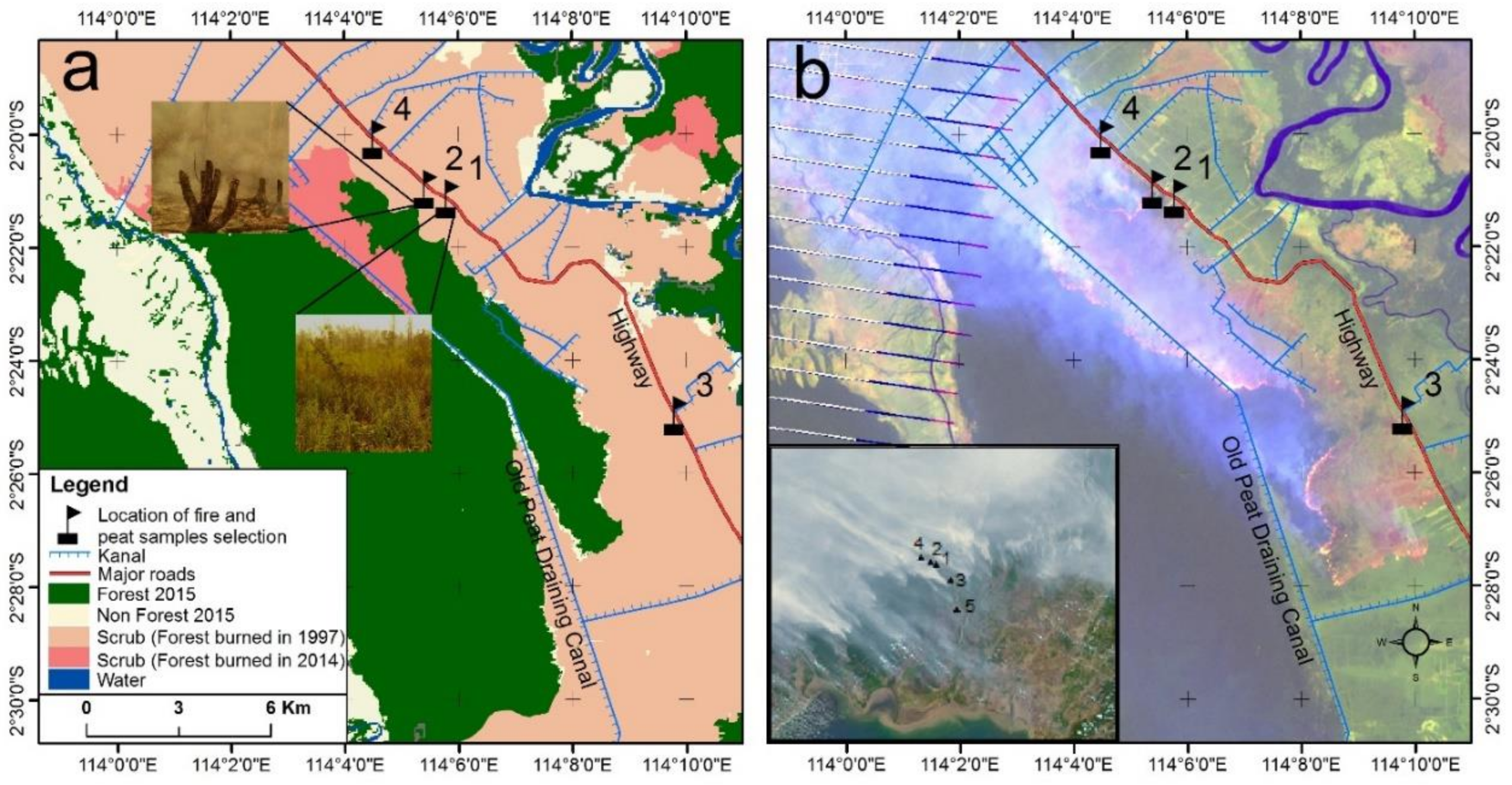
Loc. 1: 12 October Close to source smoke sampling.Sub-surface peat burn. Occasional flaming from dead surface vegetation during early period.Degraded lands, left idle (not active agriculture), dominated by scrub and ferns. See left inset in Figure 3.Peat-forest burned in 1997 and ~every 3 years since.
Loc. 2: 14 October Close to source smoke sampling.Sub-surface peat fire. Occasional flaming from dead surface vegetation during early period.Young forest regrowth.Peat-swamp forest burned in 1997. No reoccurrence.
Loc. 3: 14 October Downwind smoke sampling.Large-scale fire burning in peat forest block.Peat forestNo previous evidence of burning.
Loc. 4: 15 October Downwind smoke sampling.Flaming fire burning scrubby vegetation atop peat.Degraded idle lands, dominated by scrub and ferns. See left inset in Figure 3Peat-forest burned in 1997 and ~every 3 years since.
Loc. 5: 16 October Close to source smoke sampling.Sub-surface peat fire.Degraded idle lands, dominated by scrub and ferns. See left inset in Figure 3Peat-forest burned in 1991. Burned ~every 3 years since.
Table 2. Physio-chemical properties of unburned peat collected at the locations detailed in Table 1 and mapped in Figure 3. Values for each location (mean ± standard error) are calculated from three independent samples, except for samples indicated with (n = 1) and (n = 2). Samples relate to the surface (O horizon) layer, and to depths 0–10 cm and 10–30 cm. The O horizon was absent at all locations except Location 2, and no samples are available at Location 3 because the intense forest fire (see Figure 3) rendered it inaccessible due to safety concerns.
LocationCarbon (g·kg−1)
@ Peat Depth (cm)
Nitrogen (g·kg−1)
@ Peat Depth (cm)
C:N Ratio
@ Peat Depth (cm)
Gravimetric Moisture (g·g−1)
@ Peat Depth (cm)
Surface0–10 10–30 Surface0–1010–30Surface0–1010–30Surface0–1010–30
1-/-631 ± 23617 ± 7-/-18 ± 515 ± 0-/-42 ± 1043 ± 0-/-245 ± 30459 ± 43
2564 ± 10583 ± 9 641 28 ± 125 ± 1 16 20 ± 123 ± 2 39 165 ± 6364 ± 16350 ± 13
4-/-678 ± 4645 ± 9-/-12 ± 115 ± 1-/-56 ± 443 ± 2-/-206 ± 19259 ± 9
5-/-571 ± 50 585 -/-16 ± 1 15 -/-36 ± 6 39 -/-258 ± 1223 ± 2
Mean (n = 4)564 ± 10616 ± 21622 ± 1228 ± 118 ± 215 ± 020 ± 139 ± 641 ± 1165 ± 6268 ± 29322 ± 46
Table 3. Trace gas and particulate emission ratios for each plume sampled at the fixed measurement locations listed in Table 1 and mapped in Figure 3. Means ± 1σ, along with mean MCE ( MCE ¯ ) , are shown for each location, along with those of all plumes and the peat-only fire plumes in the final rows. Trace gas ERs are presented in units of mole·mole−1, whilst particulate to trace gas emission ratios (final three columns) are presented in units of mg·mg−1 based on standard temperature and pressure [25 °C, 1 atm.] conversion factors of 0.556 and 0.873 mg·m−3·ppm−1 for CO2 and CO respectively.
Trace Gas Emissions Ratio (ER)
[mol·mol−1]
Particulate Emissions Ratio
[mg·mg1]
PlumeCO to CO2
ER × 100
CH4 to CO2
ER ×1000
CH4 to CO
ER ×100
PM2.5 to COPM2.5 to CO2BC to PM2.5
Location 1 116.17 ± 1.0612.82 ± 0.577.77 ± 0.210.1730.0135-
212.50 ± 1.169.80 ± 0.79 7.54 ± 0.160.1820.0138-
324.20 ± 0.8115.11 ± 0.746.28 ± 0.140.1050.0092-
423.76 ± 1.6814.47 ± 1.016.08 ± 0.130.0900.0069-
523.60 ± 2.4914.63 ± 2.076.39 ± 0.320.1120.0103-
626.64 ± 0.9816.15 ± 0.656.07 ± 0.060.1170.0138-
726.49 ± 1.1316.26 ± 0.666.13 ± 0.110.1260.0160-
821.96 ± 1.2012.98 ± 0.715.89 ± 0.100.1190.0152-
925.43 ± 0.7316.23 ± 0.436.38 ± 0.040.1320.0209-
1022.73 ± 0.9814.68 ± 0.776.46 ± 0.180.1150.0165-
1125.06 ± 0.8416.53 ± 0.846.72 ± 0.180.1190.0181-
Mean ± 1σ22.59 ± 4.41
( MCE ¯ ) = 0.82
14.52 ± 2.016.52 ± 0.080.127 ± 0.0280.014 ± 0.004-
Location 2118.42 ± 0.4011.98 ± 0.226.42 ± 0.090.0730.00760.0099
220.61 ± 0.9211.91 ± 0.605.82 ± 0.050.0970.01080.0065
321.13 ± 1.0614.64 ± 0.596.81 ± 0.130.0790.00920.0061
420.55 ± 0.9214.76 ± 0.587.08 ± 0.150.0810.00920.0054
520.21 ± 0.7911.47 ± 0.425.65 ± 0.070.0910.00960.0044
Mean ± 1σ20.18 ± 1.04
( MCE ¯ ) = 0.83
12.95 ± 1.616.36 ± 0.620.084 ± 0.0100.0167 ± 0.00200.0064 ± 0.0023
Location 3115.59 ± 1.0313.90 ± 0.928.81 ± 0.270.2000.0253-
214.70 ± 0.8712.12 ± 0.978.57 ± 0.190.2630.02900.0134
316.64 ± 0.6113.67 ± 0.638.27 ± 0.160.2380.02750.0191
419.44 ± 0.8516.75 ± 0.728.57 ± 0.130.1870.02490.0180
518.36 ± 0.9414.57 ± 1.088.13 ± 0.280.2000.02250.0099
Mean ± 1σ16.95 ± 1.95
( MCE ¯ ) = 0.86
14.18 ± 1.688.47 ± 0.060.217± 0.0310.0465± 0.00450.0121± 0.0077
Location 413.95 ± 0.274.01 ± 0.4810.08 ± 0.34---
25.64 ± 0.3011.99 ± 0.5120.98 ± 0.710.8170.02330.0136
Mean ± 1σ4.80 ± 1.20
( MCE ¯ ) = 0.95
8.00 ± 5.6415.53 ± 7.790.8170.04190.0136
Location 5125.99 ± 1.777.88 ± 0.462.95 ± 0.070.0510.00670.0264
230.83 ± 1.809.05 ± 0.80 2.97 ± 0.150.0680.01170.0104
336.48 ± 1.009.92 ± 0.332.74 ± 0.080.0640.00860.0112
429.33 ± 1.738.57 ± 0.702.99 ± 0.110.0480.00710.0104
527.66 ± 1.097.06 ± 0.462.61 ± 0.910.0190.00320.0178
630.77 ± 0.747.80 ± 0.302.50 ± 0.090.0220.00300.0201
727.14 ± 1.468.40 ± 0.443.04 ± 0.090.0490.00630.0119
Mean ± 1σ29.74 ± 3.48
( MCE ¯ ) = 0.77
8.38 ± 0.84 2.82 ± 0.220.045 ± 0.0190.0120 ± 0.00550.0154 ± 0.0062
Mean of All Locations18.85 ± 9.16
( MCE ¯ ) = 0.84
11.61 ± 3.177.94 ± 4.700.225 ± 0.2790.0285 ± 0.0151 0.012 ± 0.004
Mean of Peat Only Fires
(Locations. 1, 2 and 5)
24.17 ± 4.97
( MCE ¯ ) = 0.81
11.94 ± 3.205.23 ± 2.090.085 ± 0.0410.018 ± 0.007 0.011 ± 0.006
Table 4. Per-plume trace and particulate emission factors for Locations 1 to 5 of Table 1 (mapped in Figure 4), along with their locational means ± 1σ and the overall intra-site mean and standard deviation. All trace gas data come from the laser absorption spectrometer measurements, apart from those in the row labelled “OP-FTIR” which are derived from the open path Fourier transform infrared spectrometer measures.
Trace Gas Emissions Factors [g·kg−1]Particulate Emissions Factors [g·kg−1]
PlumeCO2COCH4PM2.5 (with CO as Reference Species)PM2.5 (CO2 as Reference)BC (CO as Reference)BC (CO2 as Reference)
Location 111903 ± 157196 ± 218.89 ± 0.8333.92 ± 8.9325.68 ± 4.40--
21970 ± 163157 ± 197.04 ± 0.8128.40 ± 9.9327.27 ± 4.67--
31778 ± 146274 ± 249.80 ± 0.9428.68 ± 5.1416.33 ± 2.79--
41785 ± 148270 ± 299.42 ± 1.0224.47 ± 4.7312.41 ± 2.13--
51787 ± 151268 ± 369.53 ± 1.5730.12 ± 8.9318.53 ± 3.19--
61743 ± 143295 ± 2710.26 ± 0.9434.62 ± 9.9324.2 ± 4.14--
71745 ± 144294 ± 2710.34 ± 0.9537.17 ± 6.2727.94 ± 4.78--
81813 ± 150253 ± 258.58 ± 0.8530.27 ± 6.0427.2 ± 4.74--
91759 ± 145285 ± 2510.41 ± 0.9037.58 ± 6.4436.79 ± 6.29--
101800 ± 148260 ± 249.63 ± 0.9429.97 ± 5.7229.85 ± 5.11--
111764 ± 145281 ± 2510.63 ± 1.0333.43 ± 5.8331.99 ± 5.47--
Mean EF ± 1σ
[MCE = 0.82]
1775 ± 24275.6 ± 14.59.8 ± 0.631.8 ± 0.625.0 ± 7.9--
OP-FTIR
Flaming fire1793 ± 226271 ± 346.39 ± 0.81
Smolder fire1764 ± 223285 ± 368.60 ± 1.09
Location 211868 ± 153219 ± 198.16 ± 0.6916.03 ± 2.9714.35 ± 2.450.071 ± 0.0170.063 ± 0.014
21835 ± 151241 ± 237.97 ± 0.9823.35 ± 4.0020.26 ± 3.460.103 ± 0.0230.086 ± 0.020
31823 ± 150245 ± 249.73 ± 0.8919.26 ± 3.1316.28 ± 2.790.085 ± 0.0190.076 ± 0.017
41832 ± 151240 ± 229.86 ± 0.9019.40 ± 3.2816.77 ± 2.870.086 ± 0.0190.074 ± 0.017
51842 ± 151237 ± 227.77 ± 0.6921.48 ±3.6817.57 ± 3.000.095 ± 0.0220.078 ± 0.018
Mean EF ±1σ
[MCE = 0.83]
1840 ± 17236.4 ± 10.18.68 ± 1.0319.90 ± 2.7417.04 ± 2.150.0880 ± 0.01210.0753 ± 0.0085
OP-FTIR1801 ± 216264.2 ± 31.76.09 ± 0.72
Location 311911 ± 158190 ± 299.68 ± 1.0237.98 ± 7.2046.94 ± 8.020.378 ± 0.0960.492 ± 0.112
21928 ± 159180 ± 188.52 ± 0.9847.20 ± 9.6055.30 ± 9.450.469 ± 0.1210.562 ± 0.127
31894 ± 156201 ± 189.44 ± 0.8947.78 ± 8.9453.35 ± 9.120.475 ± 0.1100.510 ± 0.116
41845 ± 152228 ± 2111.27 ± 1.0542.74 ± 6.8845.69 ± 7.810.425 ± 0.0940.458 ± 0.104
51866 ± 154218 ± 219.84 ± 1.0943.71 ± 7.5043.59 ± 7.280.435 ± 0.0970.412 ± 0.994
Mean ± 1σ
[MCE = 0.86]
1889 ± 34203.4 ± 19.79.73 ± 1.1443.88 ± 3.9550.32 ± 4.720.437 ± 0.0450.487 ± 0.013
OP-FTIR1915 ± 214192 ± 246.82 ± 0.86
Location 412141 ± 17654 ± 63.46 ± 0.36----
22092 ± 17275 ± 79.14 ± 0.8461.39 ± 10.9948.71 ± 8.330.837 ± 0.1960.665 ± 0.151
Mean EF ± 1σ
[MCE = 0.95]
2117 *2 ± 3564.5 *2 ± 14.96.30 *2 ± 4.0261.39 *2 ± 10.9948.71 *2 ± 8.330.837 ± 0.1960.665 ± 0.151
OP-FTIR2180 ± 27521.94 ± 2.777.77 ± 0.98
Location 511763 ± 147292 ± 315.07 ± 0.5114.89 ± 2.6511.56 ± 1.980.178 ± 0.0430.142 ± 0.033
21697 ± 142333 ± 345.60 ± 0.6822.66 ± 3.5619.95 ± 3.410.271 ± 0.0590.238 ± 0.054
31626 ± 144378 ± 335.88 ± 0.5224.20 ± 3.4214.44 ± 2,470.289 ± 0.0560.164 ± 0.037
41717 ± 143321 ± 335.36 ± 0.6315.51 ± 2.5112.15 ± 2.080.185 ± 0.0410.147 ± 0.033
51741 ± 143307 ± 284.48 ± 0.475.89 ± 1.015.57 ± 0.950.070 ± 0.0160.066 ± 0.015
61699 ± 140333 ± 284.83 ± 0.447.39 ± 1.165.07 ± 0.870.088 ± 0.0190.061 ± 0.014
71747 ± 145302 ± 305.35 ± 0.5214.78 ± 2.5410.91 ± 1.870.177 ± 0.0410.132 ± 0.032
Mean EF ± 1σ
[MCE = 0.77]
1713 ± 46323.7 ± 28.55.22 ± 0.4715.05 ± 6.8811.38 ± 5.120.180 ± 0.0820.136 ± 0.060
OP-FTIR1716 ± 214321 ± 425.21 ± 65
Mean of all Locations *31866 ± 154220.7 ± 98.28.0 ± 2.134.41 ± 18.7730.19 ± 17.620.385 ± 0.3360.341 ± 0.282
Mean of Close-to-Source “Peat Only” Fires (Locations. 1, 2 and 5)1775 ± 64279 ± 447.9 ± 2.422.25 ± 8.6317.82 ± 6.860.134 ± 0.0650.106 ± 0.043
*1 Plumes 1 and 2 at Location 1 do not contribute to the mean because they were affected by surface vegetation combustion (Figure 8). *2 MCE suggests flaming-dominated smoke, which could mean mostly burning vegetation not peat, and if so EFs for this location should be reduced by up to 20% to reflect mean vegetation carbon content rather than the mean carbon content of the peat sampled herein (this downward adjustment is applied during peatland landscape-averaged EF calculations of Section 4). *3 This mean includes all locations, whereas the mean of the close-to-source sampled ‘peat only’ fires (Locations 1, 2, and 5) is shown in the final row.
Table 5. Total carbonaceous trace gas emissions for the September–October 2015 Indonesian fire event, as reported by [12] and confirmed with the new gaseous emissions factors derived herein, and by GFEDv4.1s (0.25°) [34] and GFASv1.2 (0.5°) [33].
Trace Gas Emissions (Tg)
CO2COCH4
Top-down MOPITT and GFAS optimized, see [12]692 ± 21384 ± 183.2 ± 1.2
GFEDv4.1s786979.6
GFASv1.292211110.9
Table 6. Total dry matter (DM) fuel consumption for the September–October 2015 Indonesian fire event, as derived herein and including both peat and vegetation consumption based on the method reported by [12] (whose values are also shown). Also shown are the values provided by the widely used GFASv1.2 (0.5°) [33] and GFEDv4.1s (0.25°) [34] global fire emissions inventories. Data are shown separated by month and by island. Most of the dry matter consumed in each case is peat (e.g., 305 Tg of the 358 Tg of DM fuel consumption calculated herein). Uncertainties on the first two estimates of 358 and 387 Tg are calculated as ~30%; see [12].
Dry Matter Fuel Consumption (Tg) *1
KalimantanSumatraTotal
Sept.Oct.Sept.Oct.September–October
Derived herein, based on [12] and new in situ gaseous emissions factors1001225482358
Values from [12], based on MOPITT CO and GFAS emissions and previous gaseous EFs1081325889387
GFASv1.29495139214541
GFEDv4.1s2084214566461
*1 In addition to Kalimantan and Sumatra, [12] identify a far smaller amount of combustion occurring in West Papua, but representing no more than 5% of the total DM fuel consumption of the 2015 fires.

