Assessment of the Impact of GNSS Processing Strategies on the Long-Term Parameters of 20 Years IWV Time Series


1
Faculty of Civil Engineering and Geodesy, Military University of Technology, 00-908 Warsaw, Poland
2
Faculty of Civil and Environmental Engineering, Gdansk University of Technology, 80-233 Gdansk, Poland
*
Authors to whom correspondence should be addressed.
Remote Sens. 2018, 10(4), 496; https://doi.org/10.3390/rs10040496
Submission received: 2 March 2018
/
Revised: 16 March 2018
/
Accepted: 19 March 2018
/
Published: 21 March 2018
(This article belongs to the Section Atmospheric Remote Sensing)
Abstract
:Advanced processing of collected global navigation satellite systems (GNSS) observations allows for the estimation of zenith tropospheric delay (ZTD), which in turn can be converted to the integrated water vapour (IWV). The proper estimation of GNSS IWV can be affected by the adopted GNSS processing strategy. To verify which of its elements cause deterioration and which improve the estimated GNSS IWV, we conducted eight reprocessings of 20 years of GPS observations (01.1996–12.2015). In each of them, we applied a different mapping function, the zenith hydrostatic delay (ZHD) a priori value, the cut-off angle, software, and the positioning method. Obtained in such a way, the ZTD time series were converted to the IWV using the meteorological parameters sourced from the ERA-Interim. Then, based on them, the long-term parameters were estimated and compared to those obtained from the IWV derived from the radio sounding (RS) observations. In this paper, we analyzed long-term parameters such as IWV mean values, linear trends, and amplitudes of annual and semiannual oscillations. A comparative analysis showed, inter alia, that in terms of the investigation of the IWV linear trend the precise point positioning (PPP) method is characterized by higher accuracy than the differential one. It was also found that using the GPT2 model and the higher elevation mask brings benefits to the GNSS IWV linear trend estimation.

1. Introduction
Global navigation satellite systems (GNSS) find many uses in the field of navigation, geodesy, and geophysical research. With regard to geophysical studies, more and more effort is being put into developing methods related to climate monitoring. The usage of GNSS in atmosphere studies results from the fact that the advanced processing of GPS observations allows for estimating zenith tropospheric delay (ZTD), which can be potentially used for climate monitoring [1,2], in water vapour content estimation [3,4] or in meteorology applications [5]. This parameter contains the impact of both the hydrostatic (zenith hydrostatic delay, ZHD) and the wet (zenith wet delay, ZWD) parts of the troposphere on the GPS radio signal propagation. ZHD is characterized by slight changes in time and space, and therefore is relatively easy to model. The opposite situation occurs in the case of ZWD, because its time and space variation exhibits a similarity with the water vapour content, which is one of the most important natural greenhouse gases in the atmosphere [6]. Consequently, ZWD can be converted into integrated water vapour (IWV) or precipitable water vapour (PWV) [7,8]. Thanks to the high temporal and spatial resolution of GNSS IWV, this parameter is used in many studies related to the climate [9,10], weather forecast [11], or very long baseline interferometry of VLBI [12]. According to Ning et al. (2016) [13], the uncertainties in ZTD dominate the error budget of the IWV at the level of 75%. Therefore, it is extremely important to determine the ZTD value as reliable, because its accuracy directly affects the quality of IWV. From the beginning of GNSS permanent measurements, various methods and models have been applied to observations processing. Each of them can affect final ZTD solutions in a different way and, in consequence, the GNSS IWV/PWV time series.
ZTD is one of many unknowns that are estimated during the GNSS positioning. Its value is estimated in several steps and the first of them is adopting ZHD a priori value. Subsequently, the adopted value is mapped to the satellite direction through a mapping function dedicated to the hydrostatic delay. Then, the remaining part of the delay towards the satellite is mapped to the zenith direction using the mapping function dedicated to the wet delay. In the final step, the correction of the firstly adopted ZHD value is estimated. If the firstly adopted ZHD a priori value is correct, then the obtained correction can be identified with ZWD. The sum of ZHD and ZWD gives ZTD. Since they are various mapping functions and sources of ZHD a priori value, many studies were focused on the analysis of their possible influence on ZTD estimation. Tregoning and Herring (2006) [14] have compared ZHD from the global pressure and temperature model (GPT) [15], the standard temperature and pressure model (STP), and in the situ measurements near the GPS station. At the same time, Vey et al. (2006) [16] tested using the empirical Niell mapping function (NMF) [17] and, based on the numerical weather model (NWM), isobaric mapping function (IMF) [18]. Their work was undertaken inter alia by Steingenberger et al. (2009) [19] who have analyzed the impact of the commonly used global mapping function (GMF) [20] and Vienna Mapping Function 1 (VMF1) [21], with sourcing data from GPT and the European Centre for Medium-Range Weather Forecasts (ECMWF). In all those cases, the differences in the ZTD time series obtained according to various processing schemes were found. The fact that these kinds of differences may translate into GPS IWV time series was confirmed by Thomas et al. (2011) [22], who, next to the ZHD and the mapping function (NMF/STP compared to VMF1/ECMWF), have also verified the influence of applying the atmospheric loading model (ATML) and individual antenna calibration. The biases between the ZTD time series obtained according to the above strategies caused differences in GPS PWV. The influence of elevation-dependent errors such as antenna phase center variations [23] or the signal multipath [24] on the GPS PWV was in turn undertaken by Vey et al. (2009) [25], who have verified that changing the elevation mask from 3° to 15° caused 0.75 mm differences in obtained PWV values.
All these studies were based on up to several years of observations. Therefore, it was hard to assess whether by investigating them differences may also arise in case of long-term changes, or not. The fact that various processing strategies can result in various values of the ZTD linear trend was presented by Baldysz et al. (2016) [2]. Based on the reprocessing of 18 years of observations according to two different processing strategies, they have shown that the differences in the obtained linear trends reached up to 0.26 mm/year. Due to the lot of differences between these two strategies, it was impossible to assess which factor was most responsible for the observed changes. Studies on this issue have been taken by Dousa et al. (2017), who compared seven different reprocessing variants [26]. They differ from each other in terms of mapping function, cut-off angle, non-tidal atmospheric loading, higher-order ionospheric corrections, and sampling troposphere gradients. On the basis of 172 EPN (EUREF Permanent Network) [27] stations and at least ten years of data (max span was 1996–2014), they have verified, e.g., that ZTD linear trend values may vary from each other up to 0.12 mm/year in the case of a different mapping function and up to 0.35 mm/year in the case of using various elevation masks. These results were not compared with other in situ measurements. Therefore, it is not known which of them are more reliable. This was partly verified by Ning et al. (2016) [28], who, on the basis of 20 years of GPS observations, have shown that applying various elevation masks during GPS observations processing causes differences in long-time changes of GPS IWV. They verified that higher correlations between GPS IWV and IWV from ERA-Interim [29] occurs when a 25° elevation mask is used instead of a 10°. However, it should be kept in mind that ERA-Interim is a numerical model, and although it contains reprocessed and global coverage data, there is still lack of comparison with the in situ meteorological measurements.
In order to verify the influence of other elements of the GNSS processing strategy on the long-time changes of the GNSS IWV time series, we conducted eight reprocessings for the selected EPN stations. Among them were a mapping function, an ZHD a priori value, an elevation mask, software, and the positioning method, all of which were taken into account. Using Bernese GNSS Software 5.2 [30] and GAMIT 10.50 [31], we tested 20-years ZTD time series (01.1996–12.2015) from the 20 EPN stations. As a troposphere model, VMF1, GMF/GPT, GPT2, and NMF/STP, described in detail in section two, were used. The ZHD and GNSS IWV values were obtained on the basis of pressure and mean temperature () data from the ERA-Interim. The validation of this model with in situ measurements, as well as the estimation of errors which it can translate to GNSS IWV, are also given in section two. The final results, including mean values, annual and semi-annual oscillation, and linear trends, are presented in section three, which also contains a comparison of the observations from the radio sounding (RS) stations.
2. Methodology
2.1. Atmospheric Propagation Delay
Electromagnetic wave delay () is caused by refraction and attenuation in the troposphere and is defined by the following formula [7]:
in which is the speed of light in the vacuum, is the delay measured in the unit of time, and is the neutral atmospheric refractivity, which can be divided in hydrostatic (dry gases) and wet (water vapour) components [32]:
in which is the total air pressure in [hPa], is the temperature in [K], is the water vapour pressure in [hPa], and are the air refractivity parameters. In our study, we used their values estimated by Rüger (2002) [33], which amount to 77.689 ± 0.0094 [1/hPa], 71.295 ± 1.3 [K/hPa], and 3.75463 × 10⁻⁵ ± 0.0076 × 10⁻⁵ [K2/hPa] respectively.
In many related studies, the ZTD parameter (often used interchangeably with “zenith path delay”, abbreviated as ZPD) is analyzed as:
Both parameters can be given by the following integral along the atmospheric profile:
in which
, and are the Molar weights of dry and wet air [g/mol].
The ZHD value can be also obtained using rather the accurate Saastamoinen hydrostatic model [34,35]:
in which is the ellipsoidal latitude, and is the height in [m].
IWV can be obtained using integral along the atmospheric profile:
or using ZWD:
in which is the specific gas constant of water vapour and amounts to 461.5 [J/kg K]. is a dimensionless quantity that can be obtained from the mean weighted temperature of the atmosphere :
Several empirical relations are given to determine using linear relationships with surface temperature (), which are tuned to the specific area and season [7,35,36,37,38]. This method is easy to use but does not provide high accuracy, e.g., Bevis et. al. (1994) [35] obtained the − RMS error at the level of 4.74 K. The relative error of the parameter closely approximates the relative error of . The 1 K error of caused 0.41–0.32% error of for value between 240–300 K. This value translates into the IWV error, which amounts to 0.05–0.1 kg m−2 for the ZWD value between 0.1–0.2 m. To obtain high accuracy of , the following formula can be applied:
This formula can be only used when profiles through the atmosphere in zenith direction are available. So, it is necessary to have the RS observations or data from the numerical weather model (NWM), which in many cases may not be available, especially in the case of the RS stations that have low spatial and temporal resolution. IWV contains the same information as PWV. The only difference between these two parameters results from the fact that PWV is adjusted by water density and therefore is expressed in the unit of mm.
Both Equations (8) and (9) give the same results (if is obtained using Equation (11)), but the second one can be applied using ZWD estimated from GNSS processing. Thanks to this, GNSS data can be used to study the variability of the water vapour content in the atmosphere.
2.2. ZTD from GNSS Processing
The total tropospheric delay in direction of the satellite-slant tropospheric delay (STD) can be divided into hydrostatic (SHD) and wet (SWD) components. Both of them can be determined using mapping functions and the corresponding delays at the zenith using the following formula:
in which and are slant total delays (in the direction to the satellite) for the hydrostatic and wet part of the tropospheric delay, which are projected into zenith direction and vice versa using hydrostatic and wet mapping functions, and , which depend on the satellite elevation angle () and can be described as follows [39]:
in which are coefficients for hydrostatic and wet delays. Nowadays, mapping functions based on the concept of the Vienna Mapping Function or Global Mapping Function are commonly used in GNSS data processing. and are azimuth (-dependent gradients expressed in north and east direction, and is the gradient mapping function. The Chen and Herring gradient mapping function [40] is mostly used in GNSS data processing.
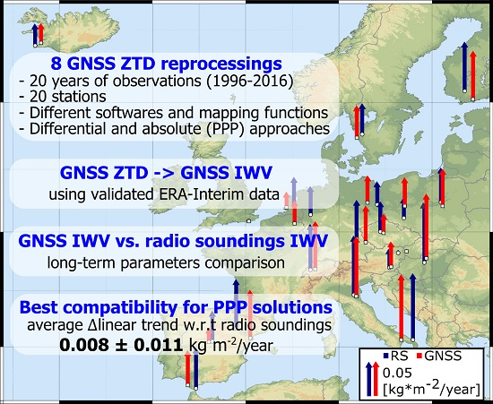
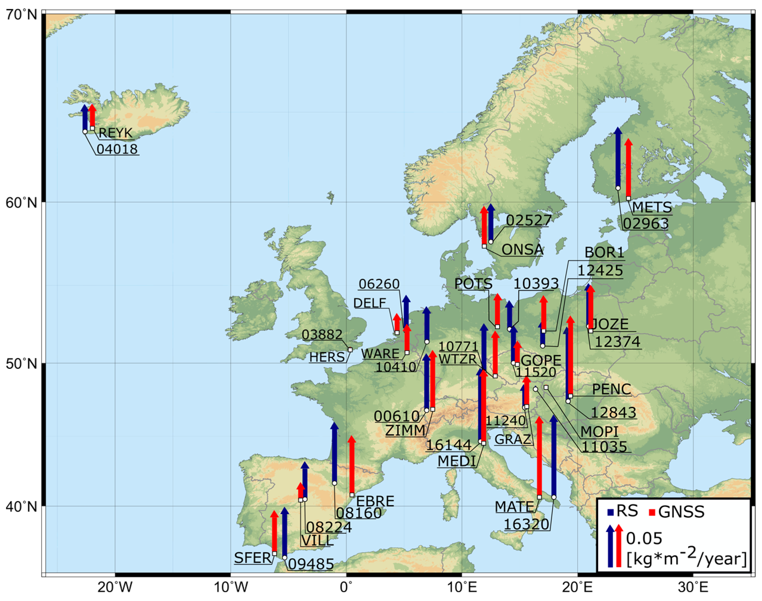
In our study, we used GPS observations from 20 EPN stations (Figure 1). Their choice was motivated by (i) an as long as possible time span of collected observations and (ii) the availability of an RS station in the range of 150 km. Selected stations operated constantly from 1996 until the end of 2015, therefore delivering 20-years of observations, which we processed according to eight different processing strategies. Four of them were conducted in Bernese GNSS Software 5.2 (with ‘BSW’ acronym) and were focused on the troposphere modelling and positioning method. For this purpose, two commonly used mapping functions with troposphere models were applied. The first of them was routinely used in EPN combination of VMF1 and ECMWF and the second was GMF/GPT. These two approaches differ from each other in terms of both mapping function and source of ZHD a priori value. In the case of VMF1 and , coefficients were adopted from NMF, and were calculated on the basis of one year of data from ERA-40 [41] through the ray-tracing procedure at 3.3° initial elevation angle ( assumed the constant value and was described by the model related to day of year and latitude). The last two coefficients of VMF1 were delivered through a ray-tracing procedure of operational weather forecasts of ECMWF at 0, 6, 12, and 18 UTC. In GMF, and were adopted from VMF1, whereas and were determined by a single ray-tracing of ERA-40 at 3.3° initial elevation angle for the 1999–2002 period of time. Therefore, the only difference between these two mapping functions occurred for and coefficients, which in VMF1 are routinely calculated and in the GMF are modelled. The same difference occurred for the ZHD a priori value. In the first combination (VMF1/ECMWF), it is sourced from the operational forecast of ECMWF, whereas in the second combination (GMF/GPT) it is estimated from the empirical model GPT, which is constructed from the same set of data as and in the GMF. These two approaches in troposphere modelling were applied in both the precise point positioning (PPP) and double difference (DD) method, and the solutions are named BSW_PPP_VMF, BSW_PPP_GMF, BSW_DD_VMF, and BSW_DD_GMF (see details in Table 1). PPP is an absolute method that allows for direct estimation of station position, whereas DD is a relative approach in which baselines between stations are estimated. Using PPP method, each station is analyzed separately, so the accuracy of final solutions are dependent mainly on the local conditions. Thanks to that, the station’s position is not affected by network related errors. However, the quality of PPP solutions strongly depends on the quality of satellite ephemerides, as well as on used models. DD method is less sensitive to quality of mentioned products, because a lot of errors are reduced during relative positioning. The main disadvantage of DD is the fact that, in contrast to the PPP, it can be affected by network related errors that can be transferred through baselines. In both these methods, conception of tropospheric delay estimation is the same.
The remaining four strategies were carried out in GAMIT 10.50 software. In the first of them (GAM_DD_VMF) we decided to apply the same combination of VMF1 and ECMWF as was used in BSW_DD_VMF in order to verify whether the internal processing scheme of both software may cause differences. This solution is also compatible with Military University of Technology (MUT) contribution to the EPN Repro2 project [42]. In the second one (GAM_DD_STP), the previously often-used NMF and STP combination was applied. The NMF coefficients for hydrostatic and wet delay were calculated based on US SA66 (US Standard Troposphere 1966) and their values are described as a function of day of the year, latitude, and station height. ZHD a priori value was, in this case, estimated on the basis of standard temperature and pressure and the Saastamoinen formula. This choice was motivated by the fact that this troposphere model was used in the first official reprocessing of EPN and may be responsible for some of the differences founded by Baldysz et al. (2016) [2]. The last reprocessing concerned troposphere modelling based on the GPT2 [43] model (GAM_DD_GPT2). This model does not have to be used together with mapping function, because it delivers both a priori ZHD and and coefficients. It was built on the same numerical model as GPT, but, in contrast to its predecessor, 10 years of data (2001–2010) were used for this purpose. It is also characterized by higher horizontal and vertical resolution. The fourth reprocessing was exactly the same as GAM_DD_VMF, but instead of the 5° cut-off angle we adopted 20° and named this solution GAM_DD_EL20.
All of the above reprocessings were conducted using reprocessed ephemerides from CODE [44]. In each case, also higher order ionospheric corrections were included in the calculation process, since their impact on the GNSS solutions was tested [45,46] and finally recommended for IGS or EPN analysis. As an antenna model, we used the type mean models (IGS08), and calculated solutions were expressed in the IGb08 frame. On the basis of obtained hourly ZTD, we calculated the daily ones using only these values whose formal estimation error was within the 3σ criterion. In next step, they were converted to the IWV by using formulas described in Section 2.1 and Equation (13) from Section 2.2. Finally, we estimated the annual and semi-annual oscillations and linear trends for each GNSS station and solution. This was done according to the following model:
in which is the observed time series, is the linear trend, and etc. are coefficient for the condition of sine and cosines using the method of least squares. The number of concerned sine and cosine conditions was chosen individually for each station by making Lomb-Scargle periodograms [47].
2.3. Meteorological Parameters
As we mentioned before, to calculate IWV from ZTD the meteorological parameters such as surface pressure (to estimate ZHD from the Saastamoinen model (7) and therefore ZWD (3)) and (to calculate IWV from ZWD (11)) are necessary. Unfortunately, there are not many GNSS stations equipped with meteorological sensors, and, even in the case of the ones that are, the quality of this data and its completeness are questionable. Thus, it is a problem to obtain reliable meteorological data on GNSS station location.
In several studies [3,48,49], data from neighboring synoptic stations are interpolated to the localization of the GPS station and then are used in further analysis. Such an approach allows for obtaining surface pressure and , which is calculated from the relationship. However, obtained in such way is not characterized by very high accuracy and therefore may cause errors during the ZWD to IWV conversion. Data from synoptic stations are not suitable for estimation according to Equation (11) due to the fact that they do not provide temperature and humidity profiles (or dew point temperature). Such profiles can be obtained using radiosondes or microwave measurements. Unfortunately, their spatial distribution is not sufficient enough to make it possible to use them in all cases. For example, on the Polish territory they are only 3 sounding stations, whereas GNSS permanent stations are more than 400. Therefore, we decided to use meteorological data sourced from the ERA-Interim (Dee et al., 2011) [29]. This model allowed us obtain data from 1979 to the present with about 80 km and 6 h of spatial and temporal resolution, respectively. Its advantage is also the possibility of getting various profiles up to 0.1 hPa level. What is more, the ERA-Interim data are re-analyzed, so it can be stated that they are continuous.
Based on the ERA-Interim data, we calculate surface pressure () on the GNSS station locations using the following steps: (i) firstly, four grid nodes nearest to the GNSS station are selected; (ii) at these nodes is converted to sea pressure () using Equation (15); and (iii) then, is interpolated at the GNSS latitude and longitude using bilinear interpolation [50] and converted to using transformed Equation (13).
In the case of based on the ERA-Interim profiles, we estimated using Equation (11) and then performed a bilinear interpolation to obtain its value at the GNSS station location. We did not apply any height corrections.
To validate our methodology and to check ERA-Interim accuracy, we performed a comparison to the in situ measurements based on the soundings stations. We selected 20 sounding stations located as close as possible to the analyzed GNSS stations. In Table 2, we present these stations together with the distance to the nearest GNSS stations. The location of the sounding stations are also shown in Figure 1.
Our comparison was made based on the same 20-year time range for which we analyzed the GNSS data. In Table 3, detailed differences between the measured and modeled parameters are shown. It can be noticed that the maximum pressure bias was obtained for station 04018 and amounted to −1.26 hPa. Based on Equation (7), it can be seen that this value corresponds to about −2.9 mm of ZHD. If we look at the absolute mean value of we can notice that the impact of wrong modeled pressure on ZHD is smaller and amounts to about 1.1 mm. Better results were obtained for annual and semiannual amplitudes and linear trend in which the absolute mean differences amounts to 0.10 hPa, 0.05 hPa, and 0.02 hPa/year respectively, which is around 0.2 mm, 0.1 mm, and 0.05 mm/year of ZHD. It should be remembered that these values, which can be called errors caused by the meteorological model, translate directly to ZWD and further to the IWV value.
In the case of , we see that the biggest bias, 1.71 K, is for station 08160. For = 270 K and ZWD = 0.1 m, this value caused about 0.1 kg m−2 differences of IWV. As we can see, the absolute mean value is much smaller (0.55 K) and hence the impact on IWV is also smaller (about 0.03 kg m−2). Based on these considerations, we state that the impact of wrong modeled and interpolated can be neglected, because the obtained absolute mean of (0.01 K) translates to IWV at the level of about 0.0006 kg m−2/year.
To assess how the modeled and interpolated and affect the IWV, we made a calculation based on Equations (7), (9), and (10). Values from Table 3 ( and ) were used to estimate errors of ZHD (which translates to ZWD (3)) and . Then, using the mean value of and ZWD derived from the sounding observations ( and respectively), we calculated the differences of mean IWV (), the amplitude of annual () and semiannual () oscillations, and the linear trend (). All results we show in Table 4.
Based on the results presented in Table 4, we state that the used source of meteorological data (the ERA-Interim), as well as the adopted interpolation methods, give results that can be used for further analysis. In our research we mostly pay attention to long-term parameters such as oscillation amplitudes and trend. As it is seen in Table 4, the used meteorological parameters do not affect them strongly (0.05 kg m−2, 0.02 kg m−2, and 0.006 kg m−2/year, for annual and semiannual oscillations, and linear trend, respectively). As it will be seen later in our paper, the obtained absolute mean differences are below the GNSS IWV statistic parameters estimation error. Slightly worse results were obtained for in which the biggest value is for station 04018. This is not surprising, because for this station also the biggest was noticed (Table 3). Even so, this value is still acceptable, the more that absolute mean is only 0.16 kg m−2. In spite of all, due to large distance between GNSS and the soundings stations, and the height differences between them, in our paper we did not analyze in detail the total value of IWV. We believe that these distances do not significantly affect the differences in trend and average amplitudes.
3. Results
In this section, we present our analysis of the calculated GNSS IWV time series. The mean differences between GNSS IWV and IWV from RS are present in this section. Subsequently, the inter-annual variations of GNSS IWV, in terms of annual and semi-annual components, and their comparison to the RS IWV are presented. Finally, we would like to draw the greatest attention to the analysis of long-term differences between all conducted reprocessings, in particular to their validation using RS observations. The comparison between GNSS IWV and RS IWV was made only for days in which data were available of both solutions.
3.1. Mean IWV
The selected GNSS stations were characterized by various prevailing humidity conditions. The mean IWV values from all analyzed GNSS IWV solutions were in the range of 12.07 kg m−2 to 22.05 kg m−2 (Table A1 in Appendix). These results were consistent with those obtained from RS IWV, which were in the range of 11.46 kg m−2 to 19.51 kg m−2 (Table A2 in Appendix). Although both GNSS IWV and RS IWV were characterized by a similar mean value, it can be noticed that the RS results were slightly lower than the GNSS ones. This is visible in Figure 2, in which differences between them are given. Only for two stations (MATE, MOPI), the mean GNSS IWV was clearly lower than the mean IWV from the corresponding RS stations. For the MATE and 16320, the height difference is at the level of 480 m, whereas for the MOPI and 11035 it is 335 m. Therefore, the characteristic decrease in air humidity with increasing height can be noticed here. Generally, absolute mean differences between GNSS IWV and RS IWV were smaller than 1.50 kg m−2 (only in the case of one solution it was 1.51 kg m−2) (Table A3 in Appendix). Among all stations, the biggest similarity between the GNSS and RS results occurred for the GRAZ and 11,240 stations. In this case, all of the Bernese solutions were below 0.25 kg m−2, and only two GAMIT solutions were higher than 0.50 kg m−2. This consistency results mostly from the small distance between the GNSS and RS station, which is only 9 km. Analogical situation occurred in the case of HERS and 03882, which had differences in the mean IWV value at the level of 0.57 kg m−2. These two stations are only 4 km away from each other. On the other hand, PENC, SFER, and BOR1 with corresponding values of 12843, 08495, and 12425 are several dozen kilometers from each other (up to 130 km) and are still characterized by one of the smallest discrepancies with respect to (w.r.t.) RS. The biggest differences occurred for the EBRE and 08160 stations and reached up to 5.37 kg m−2. These stations are in the 147 km distance at the various station heights (Δh = 200 m). This probably caused reducing of the Mediterranean water masses influence on the local humidity conditions for the inland localized 08160 station. There were also other pairs of GNSS and RS stations that were a large distance from each other, like in the case of BOR1 with 12425 and WARE with 10410. However, in contrast to the EBRE and 08160 stations, they are characterized by much smaller height differences, which were at the level of 27 m and 11 m (Table 3). An interesting situation occurred for MEDI and corresponding 16144. These two stations are 15 km from each other, and the ΔH for them is about 1 m, but still, differences in the mean IWV between them were higher than in the case of the stations separated by a much larger distance. This situation was confirmed by each of the GNSS solutions, so probably there occurred some local conditions that affected the GNSS observations in that way. On the other hand, it has to be also kept in mind that all differences between RS and GNSS may be partly caused by the model uncertainties. As it was shown in Table 4, differences of the mean IWV value between the ERA-Interim and RS observations varied from −0.44 kg m−2 to 0.43 kg m−2 (observations-ERA-Interim). Due to the fact that in our conversion from ZTD to IWV we sourced meteorological parameters from the ERA-Interim, the uncertainties of the model may translate to the uncertainties of those calculated from GNSS IWV.
3.2. IWV Amplitudes
Because they took place in the mean IWV, the values of the annual oscillations did not significantly vary between the particular GNSS solutions (Figure 3) (Table A4 in Appendix). More precisely, the biggest discrepancies were found for the MOPI station and amounted to 0.33 kg m−2 (GAM_DD_STP and GAM_DD_EL20) (Table A5 in Appendix). This value makes up about 4% of the total value of the annual component for this station and is the greatest deviation from all solutions both in terms of absolute and relative term. The rest of the stations were in the range of 0.04 kg m−2 to 0.27 kg m−2, which means that for most of them all GNSS solutions differ from each other by less than 3%. By comparing these results to the annual amplitudes from the RS, it can be noticed that various stations were characterized by various similarities to the RS. Firstly, there were stations for which the estimated values of the annual component on the basis on GNSS and RS were practically the same. DELF and 06260 may serve as an example. Obtained in this case the differences were usually below the value of the estimated for ERA-Interim accuracy (Table 4), which was at the level of 0.02 kg m−2. A similar situation occurred in the cases of BOR1, JOZE, WARE, and WTZR with corresponding values of 12425, 12374, 10410, and 10771. The annual amplitude values obtained from them mostly differ by less than the model accuracy and less than the annual amplitude estimation error, which was at the level of 0.06 to 0.09 kg m−2. On the other hand, there were stations like EBRE and 08160, which annual amplitudes differ about 2.79 kg m−2. For this pair of stations, we found also the biggest differences in the mean IWV value. However, next to EBRE, also GOPE, GRAZ, MATE, MOPI, and ZIMM stations where characterized by higher discrepancies w.r.t. RS stations. Similar to EBRE, each of them is at a long distance from the corresponding RS station, and, probably, this is the reason of the various annual signals. The only exception to this is the GRAZ station, which is located only 144 m higher than the corresponding 11240 station. The height difference between these two stations seems not to be big compared to the other mentioned cases. For example, the height difference between MOPI and 11035 is 335 m, and between MATE and 16320 it is 480 m. However, GRAZ and 11240 are situated in the Alps. Therefore, their local weather conditions are mountainous, which could cause the occurrence of the obtained differences despite the relatively small difference in height. The EBRE and 08160 stations varied from the mentioned cases, most probably due to the fact that, apart from the differences in height, they are also separated by big distance, so local weather conditions may also be completely different. The fact that the obtained results between GNSS and RS seem to be logical and explainable confirms the usefulness of GNSS in the investigation of changing prevailing weather conditions.
Next to the annual amplitudes, we also estimated the values of semiannual signal for each of the analyzed solutions (Table A6 in Appendix). From all of the strategies, only those based on the PPP mode gave in the case of the SFER station a slightly higher value of semiannual amplitude than the rest of the analyzed time series. By comparing them to the RS (Table A7 in Appendix), it can be noticed that in the vast majority of cases differences between GNSS and RS were below 0.10 kg m−2. Only in the case of EBRE and the mentioned SFER station, they were higher and amounted to 0.6 kg m−2 and 0.3 kg m−2, respectively.
3.3. IWV Linear Trend
An analysis of the obtained results showed that there was a much smaller consistency in the linear trend value between the GNSS solutions (Table A8 in the Appendix and Figure 4). Depending on the station, the obtained differences in linear trend varied from 0.015 kg m−2/year, like in the case of BOR1, to 0.121 kg m−2/year, like in the case of SFER. By complementing these values with the value of the linear trend estimation error (0.006–0.008 kg m−2/year), it can be noticed that the mentioned differences were significant and not random. Therefore, they have to result (at least partly) from the adopted GNSS observation processing strategy. Similar to in the previous analysis, we compared the obtained results to the RS results. As it can be seen in Table A9 and Figure 5, the most convergent to the RS linear trend values were those obtained from the PPP solutions (BSW_PPP_VMF and BSW_PPP_GMF). Both in the case of applying GMF and VMF1, the absolute mean value of the differences between these two solutions and the RS solutions were at the level of 0.008 kg m−2/year. Also, the selected values of the linear trend in the PPP solutions did not vary much from the RS trends. As an example, for the 12 stations in BSW_PPP_VMF, the linear trend value differs from the RS linear trend by less than its estimation error, whereas in the PPP_GMF such a situation occurred in the case of even the 14 stations. High similarity between both solutions and RS is also expressed by the lowest standard deviations (SD) of differences, which were at the level of 0.011 kg m−2/year. For comparison to the PPP solutions, two other BSW solutions conducted in DD mode (BSW_DD_VMF and BSW_DD_GMF) had almost twice as high value of absolute mean difference, which amounted to 0.017 kg m−2/year for the VMF and 0.016 kg m−2/year for GMF solutions. The standard deviations were also two times higher than in the PPP solutions and amounted to 0.022 kg m−2/year. By comparing the PPP solutions to the remaining differential solutions (all GAMIT), it can be also noticed that PPP presents more reliable results. The comparison of only the differential solutions looks interesting as well. Firstly, two solutions (BSW_DD_VMF and GAM_DD_VMF) conducted according to EPN AC (Analysis Centre) guidelines seems to be characterized by similar accuracy compared to the RS solutions. Despite several cases for which they had clearly different values of linear trend (e.g., HERS, SFER), they had the same absolute mean value of differences w.r.t. RS, which was 0.017 kg m−2/year. SDs for these both solutions were not identical but were also very similar to each other and amounted to 0.022 kg m−2/year and 0.023 kg m−2/year for BSW_DD_VMF and GAM_DD_VMF, respectively. Secondly, applying the GMF/GPT combination instead of VMF1/ECMWF resulted in a slight improvement in the accuracy of the estimated linear trends. The absolute mean differences of the solution obtained on the basis of GMF/GPT were at the level of 0.016 kg m−2/year. Thirdly, applying the GPT2 instead of GMF/GPT or VMF1/ECMWF seems to bring the best results of all differential solutions. Although GAM_DD_GPT2 still represented poorer accuracy than the PPP solutions, it is clearly visible that linear trend values from this solution were more consistent with the RS linear trends than those that took place in the case of GAM_DD_VMF1. As an example, the absolute mean differences from GAM_DD_GPT2 were at the level of 0.012 kg m−2/year, whereas SD of these differences was at the level of 0.015 kg m−2/year. This solution still contained some more significant discrepancies compared to the RS trends, but the highest one amounted to −0.035 kg m−2/year (SFER). At the same time, in the BSW_DD_VMF and BSW_DD_GMF it was −0.063 kg m−2/year and −0.061 kg m−2/year (also SFER), whereas in case of GAM_DD_VMF it was 0.076 kg m−2/year (REYK). Next to the using of GPT2, also, applying higher elevation mask brings benefits to the GNSS IWV solutions. As it can be noticed from the comparison of the GAM_DD_VMF and GAM_DD_EL20, there is a reduction of absolute mean differences value (to 0.014 kg m−2/year) and SD of these differences (to 0.016 kg m−2/year). Finally, as it was expected, the solutions obtained on the basis of the NIELL/STP combination (GAM_DD_STP) were characterized by poorer accuracy. The absolute mean difference between the linear trends from this solution and from RS was the lowest from all of the GNSS solutions and amounted to 0.022 kg m−2/year.
A detailed analysis of the results showed also some aspects worth emphasizing like, e.g., differences in the case of SFER station for which BSW_DD_GMF and BSW_DD_VMF were characterized by much poorer accuracy (−0.063 kg m−2/year) than GAM_DD_VMF (0.002 kg m−2/year). Such clear discrepancies between two analogical solutions (BSW_DD_VMF and GAM_DD_VMF) occurred also in the cases of the REYK, JOZE, and HERS stations, but in these cases the solution from Bernese was more reliable. From the mentioned stations, HERS deserves special attention because it is only 4 km away from the 03882 station and the height difference between them is only 21 m. Due to the fact that it can be assumed that over both these stations there occurred similar weather conditions, the results obtained for GAM_DD_VMF are interesting. The opposite situation (higher accuracy of GAM_DD_VMF) can be found for MEDI, which is also located in close neighborhood of the corresponding RS station.
Due to the fact that both PPP solutions were deprived of such large and hardly explainable discrepancies, and were characterized by the highest consistency with RS, we decided to use them for a detailed comparison with RS. Figure 5 represents the linear trend value for BSW_PPP_VMF and RS. As can be clearly noticed from it, all the trends are positive, so in terms of trend character there is a 100% consistency between the GNSS PPP and RS method. This occurred even for stations for which we noticed the highest discrepancies in term of mean IWV or annual amplitude value, like EBRE with 08160 or MOPI with 11035. Generally, 65% of the stations were characterized by smaller discrepancies between GNSS_PPP and RS than the linear trend estimation error and 55% by less than the estimated mean ERA-Interim accuracy w.r.t. RS (from which we sourced meteorological parameters to the GNSS IWV conversion). The highest discrepancies between GNSS PPP IWV and RS IWV occurred for VILL and 08221. For the first of them, the linear trend value reached up to 0.016 kg m−2/year, whereas for the second of them it was 0.044 kg m−2/year. These stations are only 32 km away, and the height difference between them is 38 m. The estimated ERA-Interim accuracy for the 08221 station was at the level of 0.003 kg m−2/year (Table 4). Consequently, nine times greater differences in the linear trend value cannot be explained by model accuracy. They also cannot be explained by the linear trend estimation uncertainty, which was at the level of 0.006–0.008 [kg m−2/year]. Such big changes were probably not caused by real weather conditions, as well. A similar situation occurred in the case of GOPE with 11520 and GRAZ with 11240, for which no noticeable differences were found. It is difficult to assess which methods gave more reliable results; however, it is not insignificant that all these stations are at high altitudes. Perhaps there are some altitude-related aspects that caused this inconsistency.
Excluding these clearly unreliable stations, it can be noticed that rest of the differences did not have to result from numerical or environmental errors but rather represent some climatological information. As an example, linear trends obtained from the DELF and WARE stations are smaller than those corresponding to the 06260 and 10410 stations. However, if we take into account the fact that stations HERS and 03882 located to the west of them had an almost unnoticeable trend, and stations WTZR and 10771 located to the east of them had a higher trend, it can be assumed that the visible differences reflect real changes.
4. Discussion
The obtained results showed that there are differences in the analyzed GNSS IWV solutions. Generally, the short term variations of the GNSS IWV time series, like the annual amplitudes, were very consistent. The obtained differences w.r.t. RS were mostly caused by the area topography and not by the distance between the stations itself. As an example of this may serve EBRE with 08160 and WARE with 10410. In the case of the first pair of stations, which are located 147 km away from each other, we obtained the biggest differences from all analyzed stations, both in terms of annual amplitude and mean IWV value. On the other hand, stations WARE and 10410 are at 145 km distance and the differences obtained for them were much smaller. The reason of this inconsistency is the altitude difference between the EBRE and 08160 stations (Δh = 200 m) compared to WARE and 10410 (11 m). Despite this, it should be emphasized that the occurrence of the differences in seasonal components does not have to mean that there will be also discrepancies in terms of long-time changes. For example, the mentioned EBRE and 08160 stations for which the similarity between all GNSS solutions and the RS solution were at one of the highest levels.
All linear trends obtained from the analyzed solutions were positive, exactly like in the case of the estimated RS linear trends. These results were also compatible with other studies related to measuring long-term changes of IWV above Europe (for example, studies conducted by Bock et al. (2014) [51], who on the basis of several techniques have also found only positive trends in Europe, or by Ning et al. (2016) [13], who for the analogous stations that we analyzed have found positive trends as well). Generally, the highest consistency between GNSS IWV and RS IWV long-term changes was found for PPP solutions. When both VMF1 and GMF were using in the PPP mode, the absolute mean difference of the linear trends w.r.t. RS and their standard deviations was the lowest of all of the analyzed strategies. In fact, most of the differences between the PPP solutions and the RS solution were below the linear trend estimation error. It should be kept in mind here that the first several years of the analyzed time span were characterized by poor satellites orbits and clocks quality, which are crucial in the PPP method, and yet the values of the linear trends seem to be more accurate than in the differential approach. This may indicate that the long-term troposphere changes obtained from GNSS are sensitive to network effects, which are unavoidable in the double difference approach.
With the exception of the PPP solutions, the best GNSS IWV solution was the one obtained on the basis of the GPT2 model (GAM_DD_GPT2). Its advantage over the solution in which GMF/GPT model (BSW_DD_GMF) was used results probably from the differences in the NWM (Numerical Weather Model) data that were used for mapping function coefficients estimation. In the case of GPT, it was monthly mean profiles from the ERA-40 from 1999–2002 period of time (23 pressure levels), whereas in case of GPT2 model, it was monthly mean profiles from ERA-Interim from 2001–2010 period of time (37 pressure levels). In addition, GPT2 is characterized by higher horizontal resolution and estimation of semi-annual terms of temporal variability (in the GPT it is only the mean and annual terms), as well as the phase (fixed in GPT). As it was confirmed by Lagler et al. (2013) [43], these advantages of the GPT2 model lead to the improvement of estimation of annual and semi-annual stations’ height components from the radio-space geodetic techniques, for which proper estimation is correlated with proper estimation of the troposphere parameters [52]. On the other hand, it is hard to explain the advantage of this solution over the solutions that were based on the VMF1, since the empirical model like GPT2 does not take into account rapid and large weather changes. ZHDs sourced from ECMWF have been demonstrated to improve ZTDs and station height repeatability compared to the empirical models like GMF/GPT or NIELL/STP (Fund et al. 2010) [53]. However, these studies were conducted based on only one year of data from EPN, and although they confirmed the superiority of the GMF/GPT model over NIELL/STP, which was also reflected in our results, it is difficult to refer them to the investigation of long-time changes. Perhaps some effects related to the sensibility of VMF1 to the short-time weather changes are translated from one station to the other through baselines between stations. It would explain the lack of major differences between GMF and VMF1 in the PPP solutions and more visible differences when, instead of a weather prediction model, we used averaged and smoothed vales from ten years of data (a comparison of GAM_DD_VMF and GAM_DD_GPT2). Next to the mapping functions and ZHD a priori value, the elevation mask also plays an important role in the final GNSS IWV accuracy. Ning et al. [28] firstly demonstrated that its higher value has a positive impact on estimated long-term changes. Also, on the basis of our set of data we can confirm that applying a 20° elevation mask instead of the routinely used 5° increases the consistency between GNSS IWV and RS IWV. In our set of data this increase of quality was found in 75% of cases (comparison of GAM_DD_VMF and GAM_DD_EL20).
Finally, it has to be highlighted that beyond the imperfection of such indirect IWV measurements as used by us the GNSS IWV conversion formula (detailed discussed in [13]), obtained differences in linear trend values did not have to result from the differences in the GNSS and RS stations localizations or from the adopted GNSS processing strategy, but also from the inhomogeneity of the RS observations [54]. On the other hand, we do not have any other source of direct IWV observational data that would provide data for such a long time. Therefore, it seems reasonable to use the RS observations for the validation of indirect methods, but with the knowledge that some differences between them may result from a lack of RS metadata. However, the high consistency between RS IWV and GNSS IWV, especially in the case of the PPP approach, does not seem to be accidental, thus confirming the usefulness of GNSS measurements in climate studies.
5. Conclusions
In this paper we have analyzed 20 years of GNSS data that were reprocessed according to eight different processing strategies. Firstly, we have converted them to the IWV using the meteorological data sourced from the ERA-Interim. Secondly, we have validated them by using the IWV time series from neighboring RS stations. The comparative analysis concerned the mean IWV value, as well as annual and semi-annual amplitude, but mostly was focused on the linear trend. After analyzing the obtained results, we can state that:
- The highest consistency between the GNSS IWV linear trends and RS IWV linear trends was found for the PPP solutions. Both in terms of using VMF1 or GMF in PPP mode, estimated long term IWV changes were usually characterized by the highest accuracy.
- The highest differences between the GNSS PPP and RS were found only for these stations, which are located at higher altitudes. Therefore, some altitude-dependent error both for the GNSS PPP and RS methods should be considered in future works.
- DD solutions, widely regarded as the most accurate, were characterized by lower consistency w.r.t. RS than the PPP ones. The PPP solutions are realized individually, whereas the DD solutions are realized in regional network. This may indicate that, due to some network effects, the DD method may introduce to the troposphere solutions errors that affect the proper investigation of long term changes.
- GPT2 brings benefits to climate-related studies. This is probably due to the fact that this empirical model better represents long term tropospheric variations than numerical weather models like ECMWF, which are mostly focused on short-time forecasts.
Acknowledgments
This research was financed by the Faculty of Civil Engineering and Geodesy of the Military University of Technology and by the Faculty of Civil and Environmental Engineering of Gdansk University of Technology statutory research funds. Calculations were carried out at the Academic Computer Centre in Gdansk. The authors would also like to acknowledge the contribution of the COST Action ES1206.
Author Contributions
Z.B. and G.N. designed the research. Z.B. was responsible for long-term parameters estimation, results analysis, and writing the paper. G.N. was responsible for processing soundings observations and ERA-Interim data; he also took a part in the results analysis. M.F. was responsible for GNSS observations processing using Bernese GNSS Software. A.A. was responsible for GNSS observations processing using GAMIT software. All authors participated in the project and approved the final manuscript.
Conflicts of Interest
The authors declare no conflict of interest.
Abbreviations
| ATML | atmospheric loading model |
| DD | double differences |
| ECMWF | European Centre for Medium-Range Weather Forecasts |
| EPN | EUREF Permanent Network |
| EPN AC | EUREF Permanent Network Analysis Centre |
| GMF | global mapping function |
| GNSS | global navigation satellite systems |
| GPS | Global Positioning System |
| GPT | global pressure and temperature model |
| GPT2 | global pressure and temperature model 2 |
| IGS | International GNSS Service |
| IMF | isobaric mapping function |
| IWV | integrated water vapour |
| MUT | Military University of Technology |
| NMF | Niell mapping function |
| NWM | numerical weather model |
| PPP | precise point positioning |
| PWV | precipitable water vapour |
| RS | radio sounding |
| SHD | slant hydrostatic delay |
| STP | standard temperature pressure |
| SWD | slant wet delay |
| VLBI | very long baseline interferometry |
| VMF1 | Vienna mapping function 1 |
| ZHD | zenith hydrostatic delay |
| ZPD | zenith path delay |
| ZTD | zenith tropospheric delay |
| ZWD | zenith wet delay |
Appendix A

Table A1.
Mean value of IWV estimated from GNSS observations using different strategies. Estimation errors are between 0.09–0.14 kg m−2.
Table A1.
Mean value of IWV estimated from GNSS observations using different strategies. Estimation errors are between 0.09–0.14 kg m−2.
| GNSS Station | [kg m−2] | |||||||
|---|---|---|---|---|---|---|---|---|
| BSW_PPP_VMF | BSW_PPP_GMF | BSW_DD_VMF | BSW_DD_GMF | GAM_DD_VMF | GAM_DD_STP | GAM_DD_GPT2 | GAM_DD_EL20 | |
| BOR1 | 16.34 | 16.38 | 16.20 | 16.24 | 16.10 | 15.68 | 16.25 | 15.59 |
| DELF | 18.08 | 18.11 | 18.01 | 18.04 | 17.72 | 17.42 | 17.88 | 17.14 |
| EBRE | 22.01 | 22.05 | 21.76 | 21.77 | 21.69 | 20.86 | 21.64 | 20.98 |
| GOPE | 16.52 | 16.56 | 16.37 | 16.40 | 16.17 | 15.86 | 16.41 | 15.88 |
| GRAZ | 16.56 | 16.61 | 16.54 | 16.58 | 16.34 | 15.95 | 16.50 | 15.87 |
| HERS | 17.67 | 17.70 | 17.59 | 17.61 | 17.50 | 17.03 | 17.65 | 16.58 |
| JOZE | 16.48 | 16.53 | 16.45 | 16.49 | 15.94 | 15.73 | 16.20 | 16.43 |
| MATE | 17.46 | 17.45 | 17.43 | 17.44 | 17.31 | 16.71 | 17.34 | 16.62 |
| MEDI | 20.62 | 20.63 | 20.43 | 20.46 | 20.33 | 20.08 | 20.55 | 19.56 |
| METS | 12.86 | 12.91 | 12.78 | 12.82 | 12.72 | 12.34 | 12.88 | 12.07 |
| MOPI | 15.10 | 15.20 | 14.89 | 14.93 | 14.86 | 14.30 | 14.90 | 14.53 |
| ONSA | 15.19 | 15.26 | 15.06 | 15.12 | 15.08 | 14.65 | 15.11 | 14.45 |
| PENC | 17.33 | 17.35 | 17.15 | 17.17 | 17.12 | 16.84 | 17.23 | 16.66 |
| POTS | 16.18 | 16.22 | 15.99 | 16.02 | 16.10 | 15.79 | 16.28 | 15.91 |
| REYK | 13.97 | 13.94 | 13.74 | 13.71 | 13.52 | 13.28 | 13.89 | 13.49 |
| SFER | 20.01 | 19.96 | 20.07 | 20.08 | 19.52 | 19.02 | 19.89 | 19.12 |
| VILL | 17.41 | 17.46 | 17.31 | 17.35 | 17.02 | 16.52 | 17.13 | 17.00 |
| WARE | 17.14 | 17.20 | 16.99 | 17.01 | 16.90 | 16.39 | 16.92 | 16.35 |
| WTZR | 15.11 | 15.16 | 14.94 | 14.99 | 14.87 | 14.63 | 15.01 | 14.61 |
| ZIMM | 14.70 | 14.76 | 14.63 | 14.70 | 14.36 | 13.95 | 14.53 | 14.11 |
Table A2.
IWV mean value (), linear trend (), and amplitude of annual () and semiannual () oscillations estimated from RS observations.
Table A2.
IWV mean value (), linear trend (), and amplitude of annual () and semiannual () oscillations estimated from RS observations.
| RS Station | [kg m−2] | [kg m−2 /year] | [kg m−2] | [kg m−2] |
|---|---|---|---|---|
| 02527 | 13.17 ± 0.09 | 0.046 ± 0.009 | 6.96 ± 0.07 | 1.51 ± 0.07 |
| 02963 | 12.03 ± 0.09 | 0.079 ± 0.007 | 7.83 ± 0.06 | 2.04 ± 0.06 |
| 03882 | 16.94 ± 0.10 | 0.001 ± 0.009 | 6.77 ± 0.07 | 1.00 ± 0.07 |
| 04018 | 11.46 ± 0.08 | 0.029 ± 0.007 | 4.67 ± 0.06 | 1.45 ± 0.06 |
| 06260 | 16.30 ± 0.07 | 0.043 ± 0.008 | 7.02 ± 0.06 | 1.09 ± 0.06 |
| 06610 | 15.04 ± 0.08 | 0.073 ± 0.007 | 7.88 ± 0.06 | 0.96 ± 0.06 |
| 08160 | 16.68 ± 0.10 | 0.078 ± 0.009 | 7.08 ± 0.07 | 0.75 ± 0.07 |
| 08221 | 13.95 ± 0.09 | 0.044 ± 0.008 | 5.00 ± 0.06 | 0.22 ± 0.06 |
| 08495 | 19.51 ± 0.11 | 0.063 ± 0.011 | 5.52 ± 0.08 | 0.99 ± 0.08 |
| 10393 | 15.51 ± 0.07 | 0.032 ± 0.006 | 8.11 ± 0.05 | 1.37 ± 0.05 |
| 10410 | 15.46 ± 0.09 | 0.042 ± 0.008 | 7.22 ± 0.07 | 1.07 ± 0.07 |
| 10771 | 14.24 ± 0.09 | 0.060 ± 0.007 | 7.52 ± 0.06 | 1.19 ± 0.06 |
| 11035 | 17.04 ± 0.09 | 0.005 ± 0.008 | 9.27 ± 0.06 | 1.41 ± 0.06 |
| 11240 | 16.77 ± 0.13 | 0.025 ± 0.011 | 9.67 ± 0.09 | 1.28 ± 0.09 |
| 11520 | 15.26 ± 0.09 | 0.044 ± 0.008 | 8.34 ± 0.06 | 1.35 ± 0.06 |
| 12374 | 15.25 ± 0.10 | 0.052 ± 0.008 | 8.82 ± 0.07 | 1.78 ± 0.07 |
| 12425 | 15.62 ± 0.10 | 0.028 ± 0.008 | 8.63 ± 0.07 | 1.59 ± 0.07 |
| 12843 | 16.65 ± 0.10 | 0.097 ± 0.009 | 9.38 ± 0.07 | 1.36 ± 0.07 |
| 16144 | 18.83 ± 0.11 | 0.096 ± 0.011 | 9.63 ± 0.08 | 0.76 ± 0.08 |
| 16320 | 18.79 ± 0.08 | 0.109 ± 0.007 | 7.75 ± 0.06 | 0.27 ± 0.06 |
Table A3.
Differences of mean value of IWV estimated from GNSS observations using different strategies (see Table A2) and sounding observations (see Table A1).
| GNSS Station | RS Station | [kg m−2] (GNSS-RS) | |||||||
|---|---|---|---|---|---|---|---|---|---|
| BSW_PPP_VMF | BSW_PPP_GMF | BSW_DD_VMF | BSW_DD_GMF | GAM_DD_VMF | GAM_DD_STP | GAM_DD_GPT2 | GAM_DD_EL20 | ||
| BOR1 | 12425 | 0.72 | 0.76 | 0.58 | 0.62 | 0.48 | 0.06 | 0.63 | −0.03 |
| DELF | 06260 | 1.78 | 1.81 | 1.71 | 1.74 | 1.42 | 1.12 | 1.58 | 0.84 |
| EBRE | 08160 | 5.33 | 5.37 | 5.08 | 5.09 | 5.01 | 4.18 | 4.96 | 4.30 |
| GOPE | 11520 | 1.26 | 1.30 | 1.11 | 1.14 | 0.91 | 0.60 | 1.15 | 0.62 |
| GRAZ | 11240 | −0.21 | −0.16 | −0.23 | −0.19 | −0.43 | −0.82 | −0.27 | −0.90 |
| HERS | 03882 | 0.73 | 0.76 | 0.65 | 0.67 | 0.56 | 0.09 | 0.71 | −0.36 |
| JOZE | 12374 | 1.23 | 1.28 | 1.20 | 1.24 | 0.69 | 0.48 | 0.95 | 1.18 |
| MATE | 16320 | −1.33 | −1.34 | −1.36 | −1.35 | −1.48 | −2.08 | −1.45 | −2.17 |
| MEDI | 16144 | 1.79 | 1.80 | 1.60 | 1.63 | 1.50 | 1.25 | 1.72 | 0.73 |
| METS | 02963 | 0.83 | 0.88 | 0.75 | 0.79 | 0.69 | 0.31 | 0.85 | 0.04 |
| MOPI | 11035 | −1.94 | −1.84 | −2.15 | −2.11 | −2.18 | −2.74 | −2.14 | −2.51 |
| ONSA | 02527 | 2.02 | 2.09 | 1.89 | 1.95 | 1.91 | 1.48 | 1.94 | 1.28 |
| PENC | 12843 | 0.68 | 0.70 | 0.50 | 0.52 | 0.47 | 0.19 | 0.58 | 0.01 |
| POTS | 10393 | 0.67 | 0.71 | 0.48 | 0.51 | 0.59 | 0.28 | 0.77 | 0.40 |
| REYK | 04018 | 2.51 | 2.48 | 2.28 | 2.25 | 2.06 | 1.82 | 2.43 | 2.03 |
| SFER | 08495 | 0.50 | 0.45 | 0.56 | 0.57 | 0.01 | −0.49 | 0.38 | −0.39 |
| VILL | 08221 | 3.46 | 3.51 | 3.36 | 3.40 | 3.07 | 2.57 | 3.18 | 3.05 |
| WARE | 10410 | 1.68 | 1.74 | 1.53 | 1.55 | 1.44 | 0.93 | 1.46 | 0.89 |
| WTZR | 10771 | 0.87 | 0.92 | 0.70 | 0.75 | 0.63 | 0.39 | 0.77 | 0.37 |
| ZIMM | 06610 | −0.34 | −0.28 | −0.41 | −0.34 | −0.68 | −1.09 | −0.51 | −0.93 |
| Absolute mean | 1.49 | 1.51 | 1.41 | 1.42 | 1.31 | 1.15 | 1.42 | 1.15 | |
Table A4.
Annual amplitude of IWV () estimated from GNSS observations using different strategies. Estimation errors are between 0.06–0.09 kg m−2.
Table A4.
Annual amplitude of IWV () estimated from GNSS observations using different strategies. Estimation errors are between 0.06–0.09 kg m−2.
| GNSS Station | [kg m−2] | |||||||
|---|---|---|---|---|---|---|---|---|
| BSW_PPP_VMF | BSW_PPP_GMF | BSW_DD_VMF | BSW_DD_GMF | GAM_DD_VMF | GAM_DD_STP | GAM_DD_GPT2 | GAM_DD_EL20 | |
| BOR1 | 8.55 | 8.56 | 8.53 | 8.53 | 8.58 | 8.72 | 8.57 | 8.54 |
| DELF | 7.02 | 7.03 | 7.00 | 7.00 | 7.03 | 7.21 | 7.02 | 7.08 |
| EBRE | 9.85 | 9.82 | 9.86 | 9.83 | 9.89 | 9.96 | 9.84 | 9.96 |
| GOPE | 7.61 | 7.60 | 7.55 | 7.54 | 7.60 | 7.73 | 7.60 | 7.55 |
| GRAZ | 9.06 | 9.05 | 9.01 | 8.99 | 9.08 | 9.18 | 9.06 | 9.00 |
| HERS | 6.59 | 6.59 | 6.54 | 6.53 | 6.59 | 6.79 | 6.59 | 6.55 |
| JOZE | 8.75 | 8.75 | 8.72 | 8.72 | 8.82 | 8.93 | 8.81 | 8.79 |
| MATE | 6.93 | 6.92 | 6.93 | 6.91 | 6.98 | 7.00 | 6.96 | 7.02 |
| MEDI | 9.84 | 9.78 | 9.77 | 9.74 | 9.81 | 9.91 | 9.76 | 9.87 |
| METS | 7.66 | 7.70 | 7.64 | 7.66 | 7.70 | 7.83 | 7.70 | 7.64 |
| MOPI | 8.06 | 8.06 | 8.00 | 7.99 | 8.09 | 8.18 | 8.12 | 7.85 |
| ONSA | 7.32 | 7.35 | 7.31 | 7.32 | 7.35 | 7.54 | 7.33 | 7.29 |
| PENC | 9.04 | 9.04 | 9.03 | 9.02 | 9.08 | 9.19 | 9.06 | 9.04 |
| POTS | 8.00 | 8.00 | 7.98 | 7.97 | 8.03 | 8.18 | 8.00 | 7.98 |
| REYK | 4.97 | 5.00 | 4.98 | 5.00 | 4.98 | 5.15 | 4.96 | 4.95 |
| SFER | 5.30 | 5.28 | 5.29 | 5.28 | 5.26 | 5.29 | 5.26 | 5.28 |
| VILL | 5.49 | 5.45 | 5.43 | 5.40 | 5.45 | 5.52 | 5.45 | 5.46 |
| WARE | 7.15 | 7.15 | 7.13 | 7.12 | 7.19 | 7.38 | 7.18 | 7.19 |
| WTZR | 7.51 | 7.49 | 7.46 | 7.44 | 7.51 | 7.65 | 7.52 | 7.38 |
| ZIMM | 7.17 | 7.14 | 7.14 | 7.11 | 7.18 | 7.31 | 7.20 | 7.15 |
Table A5.
Differences of annual amplitude of IWV () estimated from GNSS observations using different strategies (see Table A4) and sounding observations (see Table A1).
| GNSS Station | RS Station | [kg m−2] (GNSS-RS) | |||||||
|---|---|---|---|---|---|---|---|---|---|
| BSW_PPP_VMF | BSW_PPP_GMF | BSW_DD_VMF | BSW_DD_GMF | GAM_DD_VMF | GAM_DD_STP | GAM_DD_GPT2 | GAM_DD_EL20 | ||
| BOR1 | 12425 | −0.08 | −0.07 | −0.10 | −0.10 | −0.05 | 0.09 | −0.06 | −0.09 |
| DELF | 06260 | 0.00 | 0.01 | −0.02 | −0.02 | 0.01 | 0.19 | 0.00 | 0.06 |
| EBRE | 08160 | 2.77 | 2.74 | 2.78 | 2.75 | 2.81 | 2.88 | 2.76 | 2.88 |
| GOPE | 11520 | −0.73 | −0.74 | −0.79 | −0.80 | −0.74 | −0.61 | −0.74 | −0.79 |
| GRAZ | 11240 | −0.61 | −0.62 | −0.66 | −0.68 | −0.59 | −0.49 | −0.61 | −0.67 |
| HERS | 03882 | −0.16 | −0.16 | −0.21 | −0.22 | −0.16 | 0.04 | −0.16 | −0.20 |
| JOZE | 12374 | −0.06 | −0.06 | −0.09 | −0.09 | 0.01 | 0.12 | 0.00 | −0.02 |
| MATE | 16320 | −0.82 | −0.83 | −0.82 | −0.84 | −0.77 | −0.75 | −0.79 | −0.73 |
| MEDI | 16144 | 0.22 | 0.16 | 0.15 | 0.12 | 0.19 | 0.29 | 0.14 | 0.25 |
| METS | 02963 | −0.17 | −0.13 | −0.19 | −0.17 | −0.13 | 0.00 | −0.13 | −0.19 |
| MOPI | 11035 | −1.21 | −1.21 | −1.27 | −1.28 | −1.18 | −1.09 | −1.15 | −1.42 |
| ONSA | 02527 | 0.35 | 0.38 | 0.34 | 0.35 | 0.38 | 0.57 | 0.36 | 0.32 |
| PENC | 12843 | −0.34 | −0.34 | −0.35 | −0.36 | −0.30 | −0.19 | −0.32 | −0.34 |
| POTS | 10393 | −0.11 | −0.11 | −0.13 | −0.14 | −0.08 | 0.07 | −0.11 | −0.13 |
| REYK | 04018 | 0.31 | 0.34 | 0.32 | 0.34 | 0.32 | 0.49 | 0.30 | 0.29 |
| SFER | 08495 | −0.22 | −0.24 | −0.23 | −0.24 | −0.26 | −0.23 | −0.26 | −0.24 |
| VILL | 08221 | 0.52 | 0.48 | 0.46 | 0.43 | 0.48 | 0.55 | 0.48 | 0.49 |
| WARE | 10410 | −0.07 | −0.07 | −0.09 | −0.10 | −0.03 | 0.16 | −0.04 | −0.03 |
| WTZR | 10771 | 0.04 | 0.02 | −0.01 | −0.03 | 0.04 | 0.18 | 0.05 | −0.09 |
| ZIMM | 06610 | −0.71 | −0.74 | −0.74 | −0.77 | −0.70 | −0.57 | −0.68 | −0.73 |
| Absolute mean | 0.48 | 0.47 | 0.49 | 0.49 | 0.46 | 0.48 | 0.46 | 0.50 | |
Table A6.
Semiannual amplitude of IWV () estimated from GNSS observations using different strategies. Estimation errors are between 0.06–0.09 kg m−2.
Table A6.
Semiannual amplitude of IWV () estimated from GNSS observations using different strategies. Estimation errors are between 0.06–0.09 kg m−2.
| GNSS Station | [kg m−2] | |||||||
|---|---|---|---|---|---|---|---|---|
| BSW_PPP_VMF | BSW_PPP_GMF | BSW_DD_VMF | BSW_DD_GMF | GAM_DD_VMF | GAM_DD_STP | GAM_DD_GPT2 | GAM_DD_EL20 | |
| BOR1 | 1.61 | 1.63 | 1.62 | 1.60 | 1.60 | 1.57 | 1.63 | 1.58 |
| DELF | 1.01 | 1.05 | 1.03 | 0.99 | 1.03 | 0.97 | 1.03 | 0.98 |
| EBRE | 1.29 | 1.34 | 1.35 | 1.30 | 1.32 | 1.26 | 1.33 | 1.27 |
| GOPE | 1.29 | 1.31 | 1.28 | 1.25 | 1.25 | 1.23 | 1.28 | 1.24 |
| GRAZ | 1.30 | 1.32 | 1.32 | 1.29 | 1.29 | 1.25 | 1.29 | 1.29 |
| HERS | 0.91 | 0.95 | 0.96 | 0.92 | 0.93 | 0.86 | 0.94 | 0.88 |
| JOZE | 1.83 | 1.85 | 1.85 | 1.84 | 1.78 | 1.76 | 1.80 | 1.87 |
| MATE | 0.23 | 0.24 | 0.23 | 0.21 | 0.19 | 0.21 | 0.24 | 0.16 |
| MEDI | 0.81 | 0.85 | 0.81 | 0.78 | 0.80 | 0.74 | 0.80 | 0.79 |
| METS | 1.96 | 1.98 | 1.97 | 1.95 | 1.91 | 1.90 | 1.97 | 1.93 |
| MOPI | 1.38 | 1.38 | 1.38 | 1.36 | 1.33 | 1.30 | 1.37 | 1.33 |
| ONSA | 1.54 | 1.56 | 1.54 | 1.52 | 1.50 | 1.49 | 1.56 | 1.46 |
| PENC | 1.36 | 1.38 | 1.36 | 1.34 | 1.35 | 1.31 | 1.36 | 1.33 |
| POTS | 1.40 | 1.41 | 1.38 | 1.36 | 1.38 | 1.33 | 1.39 | 1.34 |
| REYK | 1.50 | 1.53 | 1.52 | 1.50 | 1.50 | 1.45 | 1.53 | 1.42 |
| SFER | 1.29 | 1.25 | 1.14 | 1.19 | 1.13 | 1.20 | 1.14 | 1.19 |
| VILL | 0.33 | 0.32 | 0.31 | 0.33 | 0.33 | 0.38 | 0.35 | 0.35 |
| WARE | 1.05 | 1.08 | 1.06 | 1.03 | 1.04 | 0.98 | 1.05 | 0.99 |
| WTZR | 1.27 | 1.29 | 1.27 | 1.25 | 1.25 | 1.21 | 1.28 | 1.25 |
| ZIMM | 0.88 | 0.92 | 0.89 | 0.85 | 0.88 | 0.84 | 0.89 | 0.83 |
Table A7.
Differences of semiannual amplitude of IWV () estimated from GNSS observations using different strategies (see Table A6) and sounding observations (see Table A1).
| GNSS Station | RS Station | [kg m−2] (GNSS-RS) | |||||||
|---|---|---|---|---|---|---|---|---|---|
| BSW_PPP_VMF | BSW_PPP_GMF | BSW_DD_VMF | BSW_DD_GMF | GAM_DD_VMF | GAM_DD_STP | GAM_DD_GPT2 | GAM_DD_EL20 | ||
| BOR1 | 12425 | 0.02 | 0.04 | 0.03 | 0.01 | 0.01 | −0.02 | 0.04 | −0.01 |
| DELF | 06260 | −0.08 | −0.04 | −0.06 | −0.10 | −0.06 | −0.12 | −0.06 | −0.11 |
| EBRE | 08160 | 0.54 | 0.59 | 0.60 | 0.55 | 0.57 | 0.51 | 0.58 | 0.52 |
| GOPE | 11520 | −0.06 | −0.04 | −0.07 | −0.10 | −0.10 | −0.12 | −0.07 | −0.11 |
| GRAZ | 11240 | 0.02 | 0.04 | 0.04 | 0.01 | 0.01 | −0.03 | 0.01 | 0.01 |
| HERS | 03882 | −0.11 | −0.07 | −0.06 | −0.10 | −0.09 | −0.16 | −0.08 | −0.14 |
| JOZE | 12374 | 0.05 | 0.07 | 0.07 | 0.06 | 0.00 | −0.02 | 0.02 | 0.09 |
| MATE | 16320 | −0.04 | −0.03 | −0.04 | −0.06 | −0.08 | −0.06 | −0.03 | −0.11 |
| MEDI | 16144 | 0.04 | 0.08 | 0.04 | 0.01 | 0.03 | −0.03 | 0.03 | 0.02 |
| METS | 02963 | −0.09 | −0.07 | −0.08 | −0.10 | −0.14 | −0.15 | −0.08 | −0.12 |
| MOPI | 11035 | −0.04 | −0.04 | −0.04 | −0.06 | −0.09 | −0.12 | −0.05 | −0.09 |
| ONSA | 02527 | 0.02 | 0.04 | 0.02 | 0.00 | −0.02 | −0.03 | 0.04 | −0.06 |
| PENC | 12843 | 0.00 | 0.02 | 0.00 | −0.02 | −0.01 | −0.05 | 0.00 | −0.03 |
| POTS | 10393 | 0.03 | 0.04 | 0.01 | −0.01 | 0.01 | −0.04 | 0.02 | −0.03 |
| REYK | 04018 | 0.07 | 0.10 | 0.09 | 0.07 | 0.07 | 0.02 | 0.10 | −0.01 |
| SFER | 08495 | 0.30 | 0.26 | 0.15 | 0.20 | 0.14 | 0.21 | 0.15 | 0.20 |
| VILL | 08221 | 0.07 | 0.06 | 0.05 | 0.07 | 0.07 | 0.12 | 0.09 | 0.09 |
| WARE | 10410 | −0.02 | 0.01 | −0.01 | −0.04 | −0.03 | −0.09 | −0.02 | −0.08 |
| WTZR | 10771 | 0.10 | 0.12 | 0.10 | 0.08 | 0.08 | 0.04 | 0.11 | 0.08 |
| ZIMM | 06610 | −0.08 | −0.04 | −0.07 | −0.11 | −0.08 | −0.12 | −0.07 | −0.13 |
| Absolute mean | 0.09 | 0.09 | 0.08 | 0.09 | 0.08 | 0.10 | 0.08 | 0.10 | |
Table A8.
Linear trend of IWV () estimated from GNSS observations using different strategies. Estimation errors are between 0.006–0.008 kg m−2/year.
Table A8.
Linear trend of IWV () estimated from GNSS observations using different strategies. Estimation errors are between 0.006–0.008 kg m−2/year.
| GNSS Station | [kg m−2/year] | |||||||
|---|---|---|---|---|---|---|---|---|
| BSW_PPP_VMF | BSW_PPP_GMF | BSW_DD_VMF | BSW_DD_GMF | GAM_DD_VMF | GAM_DD_STP | GAM_DD_GPT2 | GAM_DD_EL20 | |
| BOR1 | 0.042 | 0.038 | 0.053 | 0.050 | 0.053 | 0.048 | 0.044 | 0.052 |
| DELF | 0.019 | 0.018 | 0.021 | 0.020 | 0.024 | 0.037 | 0.014 | 0.042 |
| EBRE | 0.077 | 0.080 | 0.088 | 0.090 | 0.095 | 0.103 | 0.089 | 0.077 |
| GOPE | 0.024 | 0.021 | 0.037 | 0.034 | 0.041 | 0.029 | 0.026 | 0.053 |
| GRAZ | 0.035 | 0.019 | 0.035 | 0.022 | 0.040 | 0.016 | 0.013 | 0.019 |
| HERS | 0.004 | 0.006 | 0.001 | 0.002 | 0.034 | 0.014 | 0.009 | 0.012 |
| JOZE | 0.057 | 0.052 | 0.062 | 0.060 | 0.092 | 0.087 | 0.052 | 0.102 |
| MATE | 0.107 | 0.111 | 0.094 | 0.099 | 0.094 | 0.137 | 0.123 | 0.125 |
| MEDI | 0.097 | 0.100 | 0.118 | 0.114 | 0.099 | 0.109 | 0.102 | 0.098 |
| METS | 0.077 | 0.076 | 0.090 | 0.088 | 0.081 | 0.098 | 0.093 | 0.108 |
| MOPI | 0.004 | 0.003 | 0.012 | 0.010 | 0.011 | 0.033 | 0.015 | 0.019 |
| ONSA | 0.048 | 0.046 | 0.056 | 0.055 | 0.049 | 0.075 | 0.051 | 0.037 |
| PENC | 0.106 | 0.103 | 0.116 | 0.113 | 0.115 | 0.133 | 0.111 | 0.126 |
| POTS | 0.039 | 0.037 | 0.057 | 0.054 | 0.003 | 0.047 | 0.038 | 0.047 |
| REYK | 0.025 | 0.041 | 0.059 | 0.066 | 0.105 | 0.035 | 0.025 | 0.011 |
| SFER | 0.052 | 0.067 | 0.000 | 0.002 | 0.065 | 0.121 | 0.028 | 0.064 |
| VILL | 0.016 | 0.015 | 0.020 | 0.017 | 0.039 | 0.090 | 0.042 | 0.063 |
| WARE | 0.031 | 0.027 | 0.028 | 0.025 | 0.054 | 0.048 | 0.024 | 0.039 |
| WTZR | 0.055 | 0.053 | 0.068 | 0.066 | 0.067 | 0.082 | 0.059 | 0.069 |
| ZIMM | 0.076 | 0.069 | 0.073 | 0.065 | 0.087 | 0.074 | 0.061 | 0.077 |
Table A9.
Differences of linear trend of IWV () estimated from GNSS observations using different strategies (see Table A8) and sounding observations (see Table A1). Lowest differences marked by green, highest by red.
| GNSS Station | RS Station | [kg m−2/year] (GNSS-RS) | |||||||
|---|---|---|---|---|---|---|---|---|---|
| BSW_PPP_VMF | BSW_PPP_GMF | BSW_DD_VMF | BSW_DD_GMF | GAM_DD_VMF | GAM_DD_STP | GAM_DD_GPT2 | GAM_DD_EL20 | ||
| BOR1 | 12425 | 0.014 | 0.010 | 0.025 | 0.022 | 0.025 | 0.020 | 0.016 | 0.024 |
| DELF | 06260 | −0.024 | −0.025 | −0.022 | −0.023 | −0.019 | −0.006 | −0.029 | −0.001 |
| EBRE | 08160 | −0.001 | 0.002 | 0.010 | 0.012 | 0.017 | 0.025 | 0.011 | −0.001 |
| GOPE | 11520 | −0.020 | −0.023 | −0.007 | −0.010 | −0.003 | −0.015 | −0.018 | 0.009 |
| GRAZ | 11240 | 0.010 | −0.006 | 0.010 | −0.003 | 0.015 | −0.009 | −0.012 | −0.006 |
| HERS | 03882 | 0.003 | 0.005 | 0.000 | 0.001 | 0.033 | 0.013 | 0.008 | 0.011 |
| JOZE | 12374 | 0.005 | 0.000 | 0.010 | 0.008 | 0.040 | 0.035 | 0.000 | 0.050 |
| MATE | 16320 | −0.002 | 0.002 | −0.015 | −0.010 | −0.015 | 0.028 | 0.014 | 0.016 |
| MEDI | 16144 | 0.001 | 0.004 | 0.022 | 0.018 | 0.003 | 0.013 | 0.006 | 0.002 |
| METS | 02963 | −0.002 | −0.003 | 0.011 | 0.009 | 0.002 | 0.019 | 0.014 | 0.029 |
| MOPI | 11035 | −0.001 | −0.002 | 0.007 | 0.005 | 0.006 | 0.028 | 0.010 | 0.014 |
| ONSA | 02527 | 0.002 | 0.000 | 0.010 | 0.009 | 0.003 | 0.029 | 0.005 | −0.009 |
| PENC | 12843 | 0.009 | 0.006 | 0.019 | 0.016 | 0.018 | 0.036 | 0.014 | 0.029 |
| POTS | 10393 | 0.007 | 0.005 | 0.025 | 0.022 | −0.029 | 0.015 | 0.006 | 0.015 |
| REYK | 04018 | −0.004 | 0.012 | 0.030 | 0.037 | 0.076 | 0.006 | −0.004 | −0.018 |
| SFER | 08495 | −0.011 | 0.004 | −0.063 | −0.061 | 0.002 | 0.058 | −0.035 | 0.001 |
| VILL | 08221 | −0.028 | −0.029 | −0.024 | −0.027 | −0.005 | 0.046 | −0.002 | 0.019 |
| WARE | 10410 | −0.011 | −0.015 | −0.014 | −0.017 | 0.012 | 0.006 | −0.018 | −0.003 |
| WTZR | 10771 | −0.005 | −0.007 | 0.008 | 0.006 | 0.007 | 0.022 | −0.001 | 0.009 |
| ZIMM | 06610 | 0.003 | −0.004 | 0.000 | −0.008 | 0.014 | 0.001 | −0.012 | 0.004 |
| Absolute mean | 0.008 | 0.008 | 0.017 | 0.016 | 0.017 | 0.022 | 0.012 | 0.014 | |
| SD | 0.011 | 0.011 | 0.022 | 0.022 | 0.023 | 0.018 | 0.015 | 0.016 | |
References
- Baldysz, Z.; Nykiel, G.; Figurski, M.; Szafranek, K.; Kroszczynski, K. Investigation of the 16-year and 18-year ZTD Time Series Derived from GPS DATA Processing. Acta Geophys. 2015, 63, 1103–1125. [Google Scholar] [CrossRef]
- Baldysz, Z.; Nykiel, G.; Araszkiewicz, A.; Figurski, M.; Szafranek, K. Comparison of GPS tropospheric delays derived from two consecutive EPN reprocessing campaigns from the point of view of climate monitoring. Atmos. Meas. Tech. 2016, 9, 4861–4877. [Google Scholar] [CrossRef]
- Hagemann, S.; Bengtsson, L. On the determination of atmospheric water vapor from GPS measurements. J. Geophys. Res. 2003, 108, 4678. [Google Scholar] [CrossRef]
- Morland, J.; Collaud Coen, M.; Hocke, K.; Jeannet, P.; Matzler, C. Tropospheric water vapour above Switzerland over the last 12 years. Atmos. Chem. Phys. 2009, 9, 5975–5988. [Google Scholar] [CrossRef] [Green Version]
- Guerova, G.; Jones, J.; Dousa, J.; Dick, G.; de Haan, S.; Pottiaux, E.; Bock, O.; Pacione, R.; Elgered, G.; Vedel, H.; et al. Review of the state of the art and future prospects of the ground-based gnss meteorology in Europe. Atmos. Meas. Tech. 2016, 9, 5385–5406. [Google Scholar] [CrossRef]
- Yong, W.; Binyun, Y.; Debao, W.; Yanping, L. Zenith Tropospheric Delay from GPS monitoring climate change of Chinese Mainland, Education Technology and Training. In Proceedings of the 2008 International Workshop on Geoscience and Remote Sensing, ETT and GRS 2008, Shanghai, China, 21–22 December 2008. [Google Scholar] [CrossRef]
- Bevis, M.; Businger, S.; Herring, T.; Rocken, C.; Anthes, R.; Ware, R. GPS meteorology: Remote sensing of atmospheric water vapor using the global positioning system. J. Geophys. Res. 1992, 97, 15787–15801. [Google Scholar] [CrossRef]
- Wang, J.; Zhang, L. Climate applications of a global, 2-hourly atmospheric precipitable water dataset derived from IGS tropospheric products. J. Geodesy 2009, 83, 209–217. [Google Scholar] [CrossRef]
- Nilsson, T.; Elgered, G. Long-term trends in the atmospheric water vapor content estimated from ground-based GPS data. J. Geophys. Res. 2008, 113, D19101. [Google Scholar] [CrossRef]
- Ning, T.; Elgered, G.; Willen, U.; Johansson, J.M. Evaluation of the atmospheric water vapour content in a regional climate model using ground-based GPS measurements. J. Geophys. Res. 2013, 118, 329–339. [Google Scholar] [CrossRef]
- Guerova, G.; Bettems, J.-M.; Brockmann, E.; Matzler, C. Assimilation of the GPS-derived integrated water vapouur (IWV) in the MeteoSwiss numerical weather prediction model. Phys. Chem. Earth Parts 2004, 29, 177–186. [Google Scholar] [CrossRef]
- Nykiel, G.; Wolak, P.; Figurski, M. Atmospheric opacity estimation based on IWV derived from GNSS observations for VLBI applications. GPS Solut. 2018, 22, 9. [Google Scholar] [CrossRef]
- Ning, T.; Wang, J.; Elgered, G.; Dick, G.; Wickert, J.; Bradke, M.; Sommer, M.; Sommer, M.; Querel, R.; Smale, D. The uncertainty of the atmospheric integrated water vapour estimated from GNSS observations. Atmos. Meas. Tech. 2016, 9, 79–92. [Google Scholar] [CrossRef]
- Tregoning, P.; Herring, T.A. Impact of a priori zenith hydrostatic delay errors on GPS estimates of station heights and zenith total delays. Geophys. Res. Lett. 2006, 33. [Google Scholar] [CrossRef]
- Boehm, J.; Heinkelmann, R. Schuh H Short note: A global model of pressure and temperature for geodetic applications. J. Geodesy 2007. [Google Scholar] [CrossRef]
- Vey, S.; Dietrich, R.; Fritsche, M.; Rülke, A.; Rothacher, M.; Steigenberger, P. Influence of mapping functions parameters on global GPS network analyses: Comparison between NMF and IMF. Geophys. Res. Lett. 2006, 33, L01814. [Google Scholar] [CrossRef]
- Niell, A.E. Global mapping functions for the atmospheric delay at radio wavelengths. J. Geophys. Res. 1996, 101, 3227–3246. [Google Scholar] [CrossRef]
- Niell, A.E. Improved atmospheric mapping functions for VLBI and GPS. Earth Planet Space 2000, 52, 699–702. [Google Scholar] [CrossRef]
- Steigenberger, P.; Boehm, J.; Tesmer, V. Comparison of GMF/GPT with VMF1/ECMWF and Implications for Atmospheric Loading. J. Geodesy 2009, 83, 943. [Google Scholar] [CrossRef]
- Boehm, J.; Niell, A.; Tregoning, P.; Schuh, H. Global mapping function (GMF): A new empirical mapping function based on numerical weather model data. Geophys. Res. Lett. 2006, 33, L07304. [Google Scholar] [CrossRef]
- Boehm, J.; Werl, B.; Schuh, H. Troposphere mapping functions for GPS and very long baseline interferometry from European Centre for Medium-Range Weather Forecasts operational analysis data. J. Geophys. Res. 2006, 111, B02406. [Google Scholar] [CrossRef]
- Thomas, I.D.; King, M.A.; Clarke, P.J.; Penna, N.T. Precipitable water vapor estimates from homogeneously reprocessed GPS data: An intertechnique comparison in Antarctica. J. Geophys. Res. 2011, 116. [Google Scholar] [CrossRef]
- Schmid, R.; Steigenberger, P.; Gendt, G.; Ge, M.; Rothacher, M. Generation of a consistent absolute phase center correction model for GPS receiver and satellite antennas. J. Geodesy 2007, 81, 781–798. [Google Scholar] [CrossRef]
- Elósegui, P.; Davis, J.L.; Jaldehag, R.T.K.; Johansson, J.M.; Niell, A.E.; Shapiro, I.I. Geodesy using the global positioning system: The effects of signal scattering on estimates of site position. J. Geophys. Res. 1995, 100, 9921–9934. [Google Scholar] [CrossRef]
- Vey, S.; Dietrich, R.; Fritsche, M.; Rülke, A.; Steigenberger, P.; Rothacher, M. On the homogeneity and interpretation of precipitable water time series derived from global GPS observations. J. Geophys. Res. 2009, 114, D10101. [Google Scholar] [CrossRef]
- Dousa, J.; Vaclavovic, P.; Elias, M. Tropospheric products of the second GOP European GNSS reproessing (1996-2014). Atmos. Meas. Tech. 2017, 10, 3589–3607. [Google Scholar] [CrossRef]
- Bruyninx, C.; Habrich, H.; Söhne, W.; Kenyeres, A.; Stangl, G.; Völksen, C. Enhancement of the EUREF Permanent Network Services and Products. Geodesy Planet Earth 2012, 136, 27–35. [Google Scholar] [CrossRef]
- Ning, T.; Elgered, G. Trends in Atmopsheric Water Vapour Content From Ground-Based GPS: The Impact of the Elevation Cutoff Angle. IEEE J. Sel. Top. Appl. Earth Obs. Remote Sens. 2012, 5. [Google Scholar] [CrossRef]
- Dee, D.P.; Uppala, S.M.; Simmons, A.J.; Berrisford, P.; Poli, P.; Kobayashi, S.; Andrae, U.; Balmaseda, M.A.; Balsamo, G.; Bauer, P.; et al. The ERA-Interim reanalysis: Configuration and performance of the data assimilation system. Q. J. R. Meteorol. Soc. 2011, 137, 553–597. [Google Scholar] [CrossRef]
- Dach, R.; Lutz, S.; Walser, P.; Fridez, P. Bernese GNSS Software Version 5.2; User Manual; Astronomical Institute, University of Bern: Bern, Germany, 2015; ISBN 978-3-906813-05-9. [Google Scholar]
- King, R.; Herring, T.; Mccluscy, S. Documentation for the GAMIT GPS Analysis Software 10.4; Technology Report; Massachusetts Institute of Technology: Cambridge, MA, USA, 2010. [Google Scholar]
- Davis, J.L.; Herring, T.A.; Shapiro, I.I.; Rogers, E.E.; Elgered, G. Geodesy by radio interferometry: Effects of atmospheric modeling errors on estimates of baseline length. Radio Sci. 1985, 20, 1593–1607. [Google Scholar] [CrossRef]
- Rüger, J.M. Refractive Index Formulae for Radio Waves. In Proceedings of the FIG XXII International Congress, Washington, DC, USA, 19–26 April 2002. [Google Scholar]
- Saastamoinen, J. Atmospheric correction for the troposphere and stratosphere in ranging satellites. In The Use of Artificial Satellites for Geodesy, Geophysical Monography No. 15; American Geophysical Union: Washington, DC, USA, 1972; pp. 247–251. [Google Scholar]
- Bevis, M.; Businger, S.; Chiswell, S.; Herring, T.A.; Anthes, R.A.; Rocken, C.; Ware, R.H. GPS Meteorology: Mapping Zenith Wet Delays onto Precipitable Water. J. Appl. Meteorol. Climatol. 1994, 33, 379–386. [Google Scholar] [CrossRef]
- Mendes, V.B. Modeling the neutral-atmospheric propagation delay in radiometric space techniques. UNB Geodesy and Geomatics Engineering Technical Report, No. 199. Available online: http://www2.unb.ca/gge/Pubs/TR199.pdf (accessed on 1 March 2018).
- Solbrig, P. Untersuchungen Uber Die Nutzung Numerischerwettermodelle Zurwasserdampf Bestimmungmit Hilfe des Global Positioning System. Ph.D. Thesis, Institute of Geology and Navigation, University FAF Munich, Neubiberg, Germany, 2000. [Google Scholar]
- Schueler, T.; Posfay, A.; Hein, G.W.; Biberger, R. A global analysis of the mean atmospheric temperature for GPS water vapour estimation. C5: Atmospheric effects. In Proceedings of the IONGPS2001—14th International Technical Meeting of Satellite Division of the Institute of Navigation, Salt Lake City, UT, USA, 11–14 September 2001. [Google Scholar]
- Herring, T.A. Modeling Atmospheric Delays in the Analysis of Space Geodetic Data. In Proceedings of the Refraction of Transatmospheric Signals in Geodesy, Delft, The Netherlands, 19–22 March 1992; Geod.: The Hague, The Netherlands, 1992. [Google Scholar]
- Chen, G.; Herring, A. Effects of atmospheric azimuthal asymmetry on the analysis of space geodetic data. J. Geophys. Res. 1997, 102, 20489–20502. [Google Scholar] [CrossRef]
- Uppala, S.M.; KÅllberg, P.W.; Simmons, A.J.; Andrae, U.; Bechtold, V.D.C.; Fiorino, M.; Gibson, J.K.; Haseler, J.; Hernandez, A.; Kelly, G.A.; et al. The ERA-40 re-analysis. Q. J. R. Meteorol. Soc. 2005, 131, 2961–3012. [Google Scholar] [CrossRef]
- Pacione, R.; Araszkiewicz, A.; Brockmann, E.; Dousa, J. EPN-Repro2: A reference GNSS tropospheric data set over Europe. Atmos. Meas. Tech. 2017, 10, 1689–1705. [Google Scholar] [CrossRef]
- Lagler, K.; Schindelegger, M.; Bohm, J.; Krasna, H.; Nillson, T. GPT2: Empirical slant delay model for radio space geodetic techniques. Geophys. Res. Lett. 2013, 40, 1069–1079. [Google Scholar] [CrossRef] [PubMed]
- Steigenberger, P.; Lutz, S.; Dach, R.; Schaer, S.; Jäggi, A. CODE Repro2 Product Series for the IGS; Astronomical Institut, University of Bern: Bern, Germany, 2016. [Google Scholar]
- Hernández-Pajares, M.; Juan, J.M.; Sanz, J.; Orús, R. Second-order ionospheric term in GPS: Implementation and impact on geodetic estimates. J. Geophys. Res. 2007, 112, B08417. [Google Scholar] [CrossRef]
- Petrie, E.J.; King Moore, P.; Lavallee, D.A. Higher-order ionospheric effects on the GPS reference frame and velocities. J. Geophys. Res. 2010, 115, B03417. [Google Scholar] [CrossRef]
- Lomb, N. Least-squares frequency analysis of unequally spaced data. Astrophys. Space Sci. 1976, 39, 448–462. [Google Scholar] [CrossRef]
- Klein Baltink, H.; van der Marel, H.; Hoeven, A.G.H. Integrated atmospheric water vapor estimates from a regional GPS network. J. Geophys. Res. 2002, 107. [Google Scholar] [CrossRef]
- Wang, J.; Zhang, L.; Dai, A.; Van Hove, T.; Van Baelen, J. A near-global, 2-hourly data set of atmospheric precipitable water from ground-based GPS measurements. J. Geophys. Res. 2007, 112, D11107. [Google Scholar] [CrossRef]
- Kirkland, E.J. Bilinear Interpolation. In Advanced Computing in Electron Microscopy; Springer: Boston, MA, USA, 2010. [Google Scholar]
- Bock, O.; Willis, P.; Wang, J.; Mears, C. A high-quality, homogenized, global, long-term (1993–2008) DORIS precipitable water data set for climate monitoring and model verification. J. Geophys. Res. Atmos. 2014, 119, 7209–7230. [Google Scholar] [CrossRef]
- Rothacher, M. Estimation of Station Heights with GPS. Int. Assoc. Geodesy Symp. 2002, 124, 81–90. [Google Scholar] [CrossRef]
- Fund, F.; Morel, L.; Mocquet, A.; Boehm, J. Assessment of ECMWF-derived tropospheric delay models within the EUREF Permanent Network. GPS Solut. 2010, 15, 39–48. [Google Scholar] [CrossRef]
- Zhai, P.; Eskride, R.E. Analyses of Inhomogeneities in Radiosonde Temperature and Humidity Time Series. J. Clim. 1996, 9, 884–896. [Google Scholar] [CrossRef]
Figure 1.
Location of GNSS (red squares) and RS (navy circle) stations used in this study.
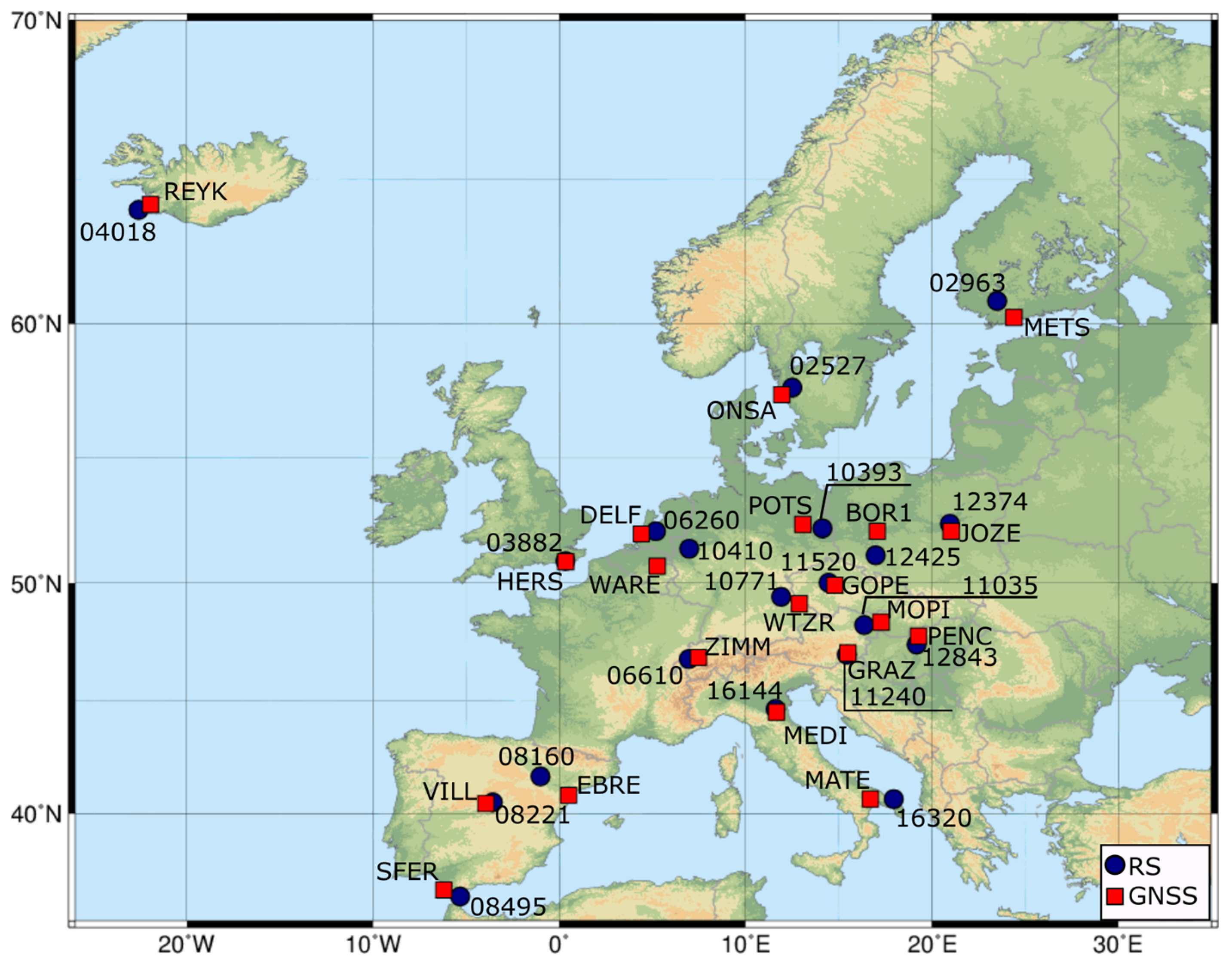
Figure 2.
Differences of mean IWV values between eight analyzed GNSS solutions and RS.
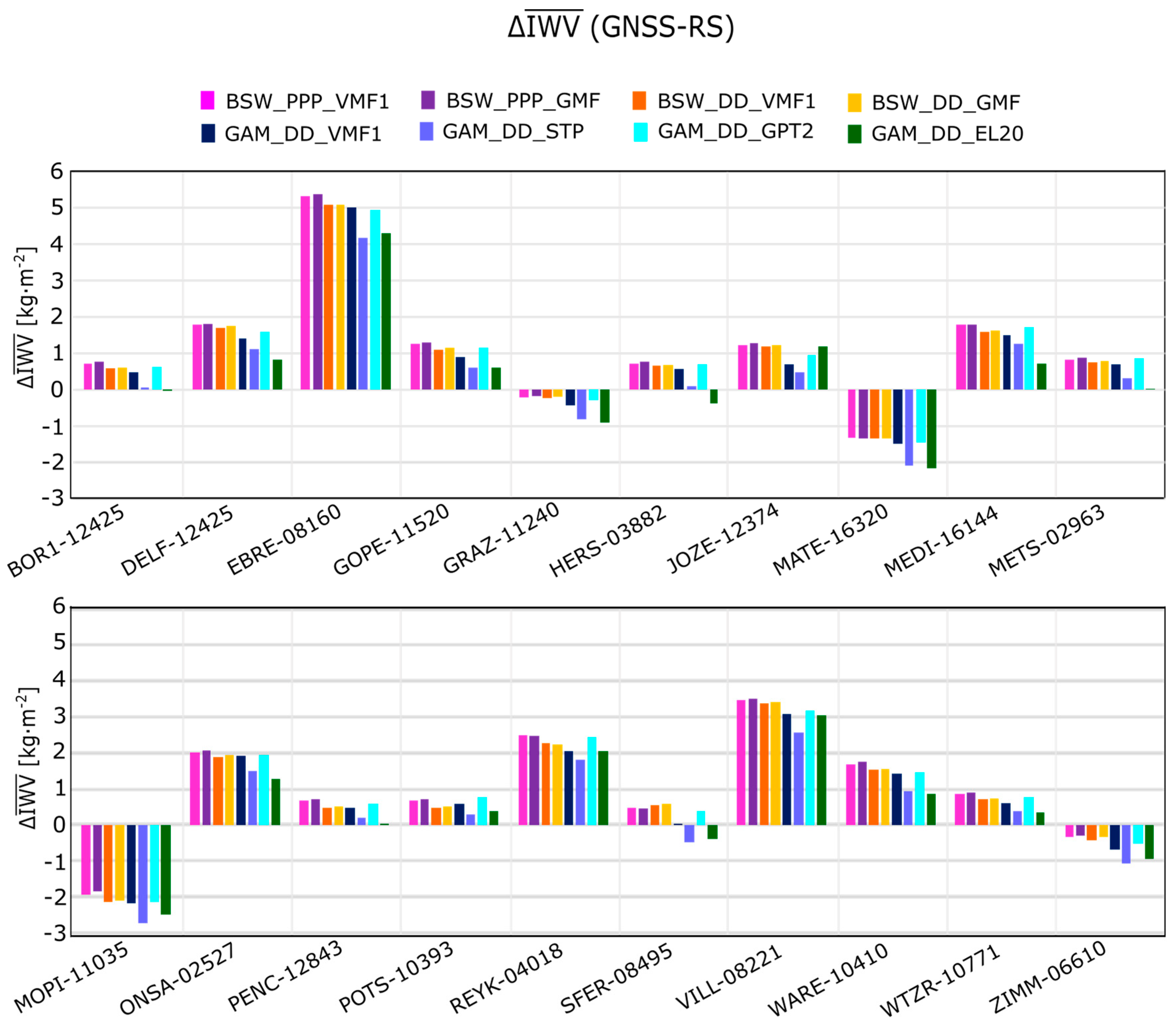
Figure 3.
Differences in IWV annual amplitude between analyzed GNSS solutions and RS.
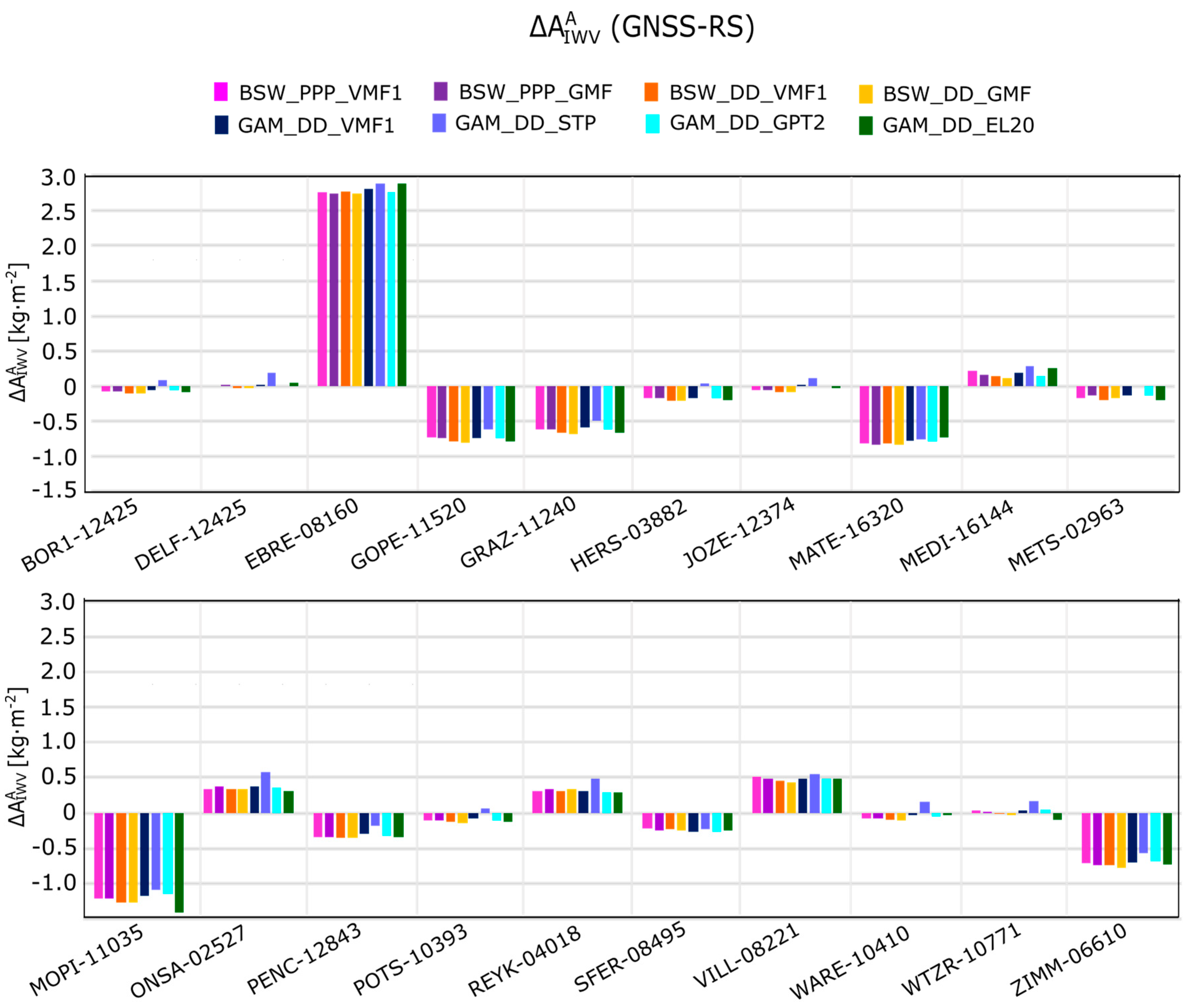
Figure 4.
Differences in IWV linear trend value between analyzed the GNSS solutions and RS.
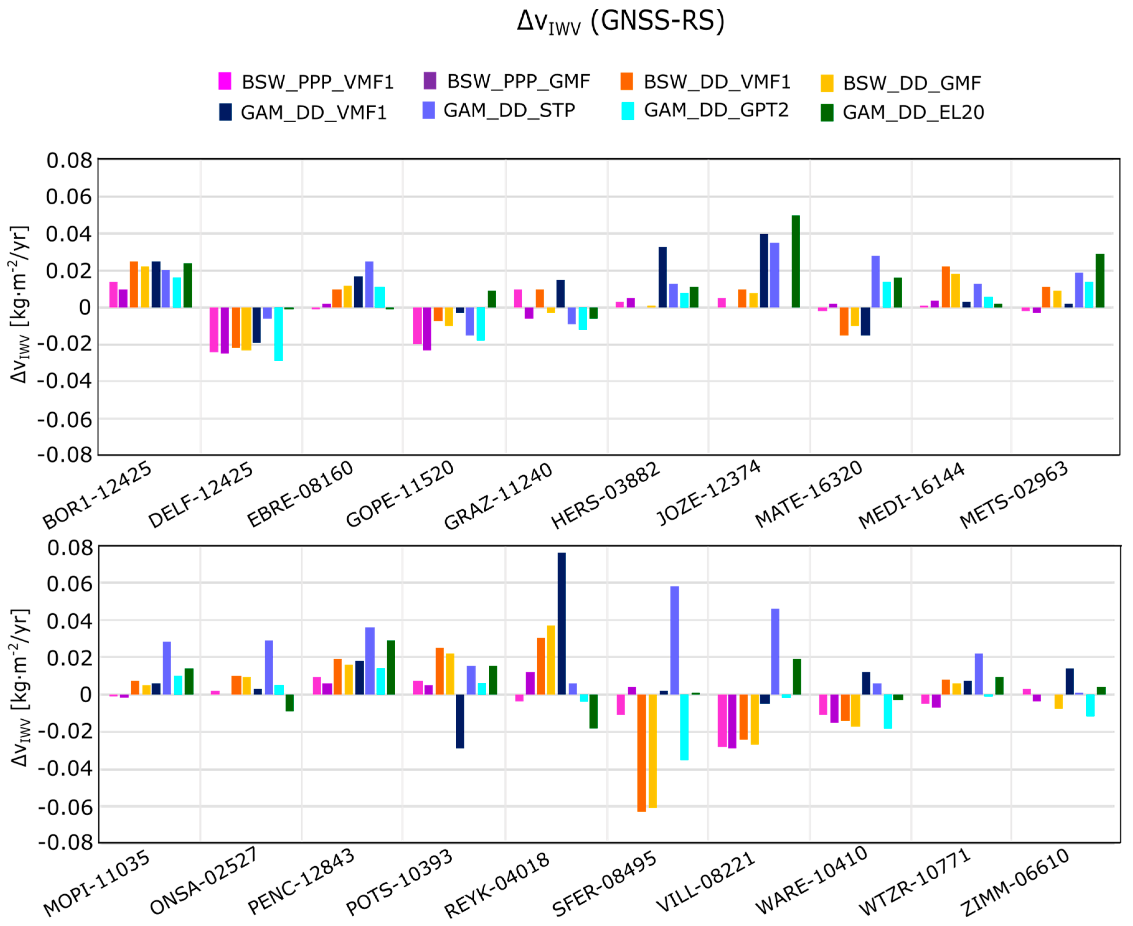
Figure 5.
Linear trend value for RS (navy) and GNSS PPP (red) for the 01.1996–12.2015 period of time.
Figure 5.
Linear trend value for RS (navy) and GNSS PPP (red) for the 01.1996–12.2015 period of time.

Table 1.
GNSS processing strategies used in this study.
| BSW_PPP_VMF | BSW_PPP_GMF | BSW_DD_VMF | BSW_DD_GMF | GAM_DD_VMF | GAM_DD_STP | GAM_DD_GPT2 | GAM_DD_EL20 | |
|---|---|---|---|---|---|---|---|---|
| software | Bernese 5.2 | Bernese 5.2 | Bernese 5.2 | Bernese 5.2 | GAMIT 10.50 | GAMIT 10.50 | GAMIT 10.50 | GAMIT 10.50 |
| method | PPP | PPP | DD | DD | DD | DD | DD | DD |
| data | daily 30-s GPS observations from 20 EPN stations (since 01.1996 to 12.2015) | |||||||
| a priori ZHD | VMF1 | GPT | VMF1 | GPT | VMF1 | STP | GPT2 | VMF1 |
| Tropo. mapping function | VMF1 | GMF | VMF1 | GMF | VMF1 | Niell | GPT2 | VMF1 |
| cut-off angle | 5° | 5° | 5° | 5° | 5° | 5° | 5° | 20° |
| High order ionospheric effects | 2nd and 3rd order | |||||||
| Ephemerides | CODE R2 (2013) | |||||||
| Antenna models | Type mean (IGS08) | |||||||
| Reference Frame | IGb08 | |||||||
Table 2.
List of GNSS and RS stations with approximate distance between them and height differences (Δh = altitude of GNSS station − altitude of RS station).
Table 2.
List of GNSS and RS stations with approximate distance between them and height differences (Δh = altitude of GNSS station − altitude of RS station).
| GNSS Station | RS Station | Approx. Distance [km] | Δh [m] |
|---|---|---|---|
| BOR1 (Borowiec, Poland) | 12425 (Wroclaw, Poland) | 130 | −27 |
| DELF (Delft, Netherlands) | 06260 (De Bilt, Netherlands) | 55 | 29 |
| EBRE (Roquetes, Spain) | 08160 (Zaragoza, Spain) | 147 | −200 |
| GOPE (Ondrejov, Czech Rep.) | 11520 (Praha, Czech Rep.) | 27 | 244 |
| GRAZ (Graz, Austria) | 11240 (Graz, Austria) | 9 | 144 |
| HERS (Hailsham, Great Britain) | 03882 (Herstmonceux, Great Britain) | 4 | −21 |
| JOZE (Jozefoslaw, Poland) | 12374 (Legionowo, Poland) | 34 | 14 |
| MATE (Matera, Italy) | 16320 (Brindisi, Italy) | 110 | 480 |
| MEDI (Medicina, Italy) | 16144 (Pietro Capofiume, Italy) | 15 | −1 |
| METS (Kirkkonummi, Finland) | 02963 (Jokioinen, Finland) | 83 | −27 |
| MOPI (Modra-Piesok, Slovakia) | 11035 (Wien, Austria) | 68 | 335 |
| ONSA (Onsala, Sweden) | 02527 (Goteborg, Sweden) | 35 | −155 |
| PENC (Penc, Hungary) | 12843 (Budapest, Hungary) | 41 | 109 |
| POTS (Potsdam, Germany) | 10393 (Lindenberg, Germany) | 74 | −11 |
| REYK (Reykjavik, Iceland) | 04018 (Keflavikurflugvollur, Iceland) | 37 | −27 |
| SFER (San Fernando, Spain) | 08495 (Gibraltar, Spain) | 84 | 36 |
| VILL (Villafranca, Spain) | 08221 (Madrid, Spain) | 32 | −38 |
| WARE (Waremme, Belgium) | 10410 (Essen, Germany) | 145 | −11 |
| WTZR (Bad Koetzting, Germany) | 10771 (Kuemmersbruck, Germany) | 78 | 201 |
| ZIMM (Zimmerwald, Switzerland) | 06610 (Payerne, Switzerland) | 40 | 416 |
Table 3.
Long-term statistics (amplitude of annual () and semiannual () oscillation, trend (, and bias) of surface pressure () and weighted mean water vapour temperature () differences between RS measurements and data derived from ERA-Interim model. Estimation errors: ; ; ; ; ; ; ; .
Table 3.
Long-term statistics (amplitude of annual () and semiannual () oscillation, trend (, and bias) of surface pressure () and weighted mean water vapour temperature () differences between RS measurements and data derived from ERA-Interim model. Estimation errors: ; ; ; ; ; ; ; .
| RS Station | (RS-Era-Interim) | (RS-Era-Interim) | ||||||
|---|---|---|---|---|---|---|---|---|
[hPa] | [hPa] | [hPa] | [hPa/year] | [K] | [K] | [K] | [K/year] | |
| 02527 | −0.07 | 0.04 | 0.02 | 0.00 | −0.77 | 0.42 | 0.12 | 0.00 |
| 02963 | −0.06 | 0.02 | 0.01 | 0.00 | −0.59 | 0.44 | 0.09 | 0.00 |
| 03882 | −0.09 | 0.01 | 0.03 | 0.04 | −0.33 | 0.19 | 0.04 | −0.03 |
| 04018 | −1.26 | 0.04 | 0.03 | −0.02 | −0.04 | 0.12 | 0.04 | −0.03 |
| 06260 | −0.60 | 0.01 | 0.03 | 0.03 | −0.53 | 0.28 | 0.03 | 0.01 |
| 06610 | −0.64 | 0.09 | 0.05 | 0.01 | 1.61 | 0.29 | 0.15 | 0.00 |
| 08160 | −0.66 | 0.12 | 0.08 | −0.01 | 1.71 | 0.27 | 0.17 | −0.04 |
| 08221 | 1.07 | 0.15 | 0.04 | 0.01 | 0.95 | 0.25 | 0.04 | −0.02 |
| 08495 | 0.29 | 0.38 | 0.10 | 0.04 | −0.22 | 0.38 | 0.03 | −0.01 |
| 10393 | 0.15 | 0.14 | 0.07 | −0.02 | −0.84 | 0.39 | 0.03 | 0.00 |
| 10410 | 0.91 | 0.03 | 0.04 | −0.02 | −0.90 | 0.41 | 0.02 | 0.03 |
| 10771 | 0.89 | 0.03 | 0.02 | −0.03 | −0.47 | 0.37 | 0.09 | 0.00 |
| 11035 | −0.20 | 0.13 | 0.04 | 0.00 | 0.20 | 0.44 | 0.12 | −0.02 |
| 11240 | 0.09 | 0.24 | 0.07 | −0.03 | 0.34 | 0.51 | 0.05 | −0.01 |
| 11520 | 0.59 | 0.03 | 0.03 | 0.00 | −0.06 | 0.33 | 0.10 | −0.01 |
| 12374 | 0.20 | 0.02 | 0.02 | 0.01 | −0.25 | 0.41 | 0.12 | −0.02 |
| 12425 | −0.45 | 0.10 | 0.03 | 0.01 | −0.10 | 0.47 | 0.07 | 0.00 |
| 12843 | −0.47 | 0.07 | 0.01 | 0.05 | −0.25 | 0.38 | 0.11 | −0.02 |
| 16144 | 0.56 | 0.07 | 0.13 | 0.01 | −0.04 | 0.31 | 0.18 | −0.01 |
| 16320 | 0.53 | 0.20 | 0.15 | 0.03 | −0.85 | 0.42 | 0.08 | 0.00 |
| abs mean | 0.49 | 0.10 | 0.05 | 0.02 | 0.55 | 0.35 | 0.08 | 0.01 |
Table 4.
Differences of mean IWV (), amplitude of annual () and semiannual () oscillations, and linear trend () caused by differences of meteorological parameters presented in Table 3.
Table 4.
Differences of mean IWV (), amplitude of annual () and semiannual () oscillations, and linear trend () caused by differences of meteorological parameters presented in Table 3.
| RS Station | [K] | [m] | [kg m−2] | [kg m−2] | [kg m−2] | [kg m−2/year] |
|---|---|---|---|---|---|---|
| 02527 | 270.58 | 0.085 | −0.06 | 0.03 | 0.01 | 0.000 |
| 02963 | 268.87 | 0.078 | −0.05 | 0.03 | 0.01 | 0.000 |
| 03882 | 274.59 | 0.108 | −0.05 | 0.02 | 0.01 | 0.012 |
| 04018 | 268.76 | 0.075 | −0.44 | 0.02 | 0.01 | −0.008 |
| 06260 | 273.88 | 0.104 | −0.24 | 0.02 | 0.01 | 0.011 |
| 06610 | 273.35 | 0.096 | −0.14 | 0.05 | 0.03 | 0.004 |
| 08160 | 278.64 | 0.105 | −0.14 | 0.06 | 0.04 | −0.006 |
| 08221 | 277.17 | 0.088 | 0.43 | 0.07 | 0.02 | 0.003 |
| 08495 | 282.10 | 0.122 | 0.09 | 0.16 | 0.04 | 0.014 |
| 10393 | 272.56 | 0.099 | 0.01 | 0.07 | 0.03 | −0.007 |
| 10410 | 273.08 | 0.099 | 0.27 | 0.03 | 0.02 | −0.005 |
| 10771 | 272.06 | 0.092 | 0.29 | 0.03 | 0.01 | −0.011 |
| 11035 | 273.81 | 0.109 | −0.06 | 0.07 | 0.02 | −0.001 |
| 11240 | 273.07 | 0.107 | 0.05 | 0.12 | 0.03 | −0.011 |
| 11520 | 272.50 | 0.098 | 0.20 | 0.03 | 0.02 | −0.001 |
| 12374 | 272.26 | 0.098 | 0.06 | 0.03 | 0.01 | 0.002 |
| 12425 | 272.53 | 0.100 | −0.16 | 0.06 | 0.01 | 0.004 |
| 12843 | 274.01 | 0.106 | −0.18 | 0.05 | 0.01 | 0.017 |
| 16144 | 277.18 | 0.119 | 0.20 | 0.05 | 0.06 | 0.003 |
| 16320 | 279.39 | 0.118 | 0.13 | 0.10 | 0.06 | 0.011 |
| Absolute mean | 0.16 | 0.05 | 0.02 | 0.006 | ||
© 2018 by the authors. Licensee MDPI, Basel, Switzerland. This article is an open access article distributed under the terms and conditions of the Creative Commons Attribution (CC BY) license (http://creativecommons.org/licenses/by/4.0/).
Share and Cite
MDPI and ACS Style
Baldysz, Z.; Nykiel, G.; Figurski, M.; Araszkiewicz, A. Assessment of the Impact of GNSS Processing Strategies on the Long-Term Parameters of 20 Years IWV Time Series. Remote Sens. 2018, 10, 496. https://doi.org/10.3390/rs10040496
AMA Style
Baldysz Z, Nykiel G, Figurski M, Araszkiewicz A. Assessment of the Impact of GNSS Processing Strategies on the Long-Term Parameters of 20 Years IWV Time Series. Remote Sensing. 2018; 10(4):496. https://doi.org/10.3390/rs10040496
Chicago/Turabian StyleBaldysz, Zofia, Grzegorz Nykiel, Mariusz Figurski, and Andrzej Araszkiewicz. 2018. "Assessment of the Impact of GNSS Processing Strategies on the Long-Term Parameters of 20 Years IWV Time Series" Remote Sensing 10, no. 4: 496. https://doi.org/10.3390/rs10040496
Note that from the first issue of 2016, this journal uses article numbers instead of page numbers. See further details here.