SAR Automatic Target Recognition Using a Roto-Translational Invariant Wavelet-Scattering Convolution Network


Key Laboratory for Information Science of Electromagnetic Waves (MoE), Fudan University, Shanghai 200433, China
*
Author to whom correspondence should be addressed.
Remote Sens. 2018, 10(4), 501; https://doi.org/10.3390/rs10040501
Submission received: 11 February 2018
/
Revised: 17 March 2018
/
Accepted: 18 March 2018
/
Published: 22 March 2018
(This article belongs to the Special Issue Analysis of Big Data in Remote Sensing)
Abstract
:The algorithm of synthetic aperture radar (SAR) for automatic target recognition consists of two stages: feature extraction and classification. The quality of extracted features has significant impacts on the final classification performance. This paper presents a SAR automatic target classification method based on the wavelet-scattering convolution network. By introducing a deep scattering convolution network with complex wavelet filters over spatial and angular variables, robust feature representations can be extracted across various scales and angles without training data. Conventional dimension reduction and a support vector machine classifier are followed to complete the classification task. The proposed method is then tested on the moving and stationary target acquisition and recognition (MSTAR) benchmark data set and achieves an average accuracy of 97.63% on the classification of ten-class targets without data augmentation.
1. Introduction
SAR automatic target recognition (ATR) is defined as employing a computerized tool to predict the class of a target in SAR images or to describe certain attributes of interest for the target, such as the geometric and physical properties of the target in the absence of direct manual intervention. A standard architecture of SAR ATR proposed by the MIT Lincoln Laboratory was described as three stages: detection, discrimination, and classification [1,2]. Detection is to extract candidate targets from SAR images using a false alarm rate (CFAR) detector. The output might include not only targets of interests but also false alarm clutter. At the following discrimination stage, in order to eliminate false alarms, several features are selected to train a discriminator to solve the two-class (target and clutter) problem. Finally, the classifier is utilized to categorize each input as a specific target type. In this paper, ‘recognition’ means the third stage, that is, classification of different types. In some applications, there is a more advanced process called the identification process, which is not discussed in this paper. Factors such as imaging angles, target configuration and background conditions have significant impacts on the SAR image classification. Therefore, extracting good feature representations that are insensitive to the above factors is particularly important to develop an effective SAR ATR system.
The basic development process of feature extraction can be divided into three stages: feature definition, feature expression and feature learning. The underlying features are initially defined based on researchers’ empirical knowledge or their own understanding of the obtained images. For example, the image is usually described by color, texture, shape or pixel statistical distribution characteristics. On the basis of the underlying features, better feature expression can be extracted by carrying out vector quantization, coding or kernel description. Dictionary learning and sparse coding are frequently used algorithms. However, features extracted from these two stages are designed or selected according to specific tasks, which requires a wealth of empirical knowledge and a deep understanding of the image. It is also time consuming and has low generalization ability.
Extracted features are then used for target classification, which includes three mainstream paradigms: template matching, a model-based method, and machine learning. In template matching, the distance is measured between the target image and the template database. A semi-automated image intelligence processing (SAIP) system is proposed [3], in which the mean square error classifier is used to find the best match between the target data and the template database. The classification accuracy of the SAIP is satisfactory if the target configuration is similar to those in the template database. There are two main disadvantages in this method: one is low efficiency in distance calculation and target searching, and the other is its performance degrades significantly when the target changes. For a model-based method, target CAD (computer-aided design) model and electromagnetic simulation software are utilized to predict SAR images of different categories and poses, which are produced by the SAR image chip to be identified. Finally a set of predicted features are compared with those extracted from the actual SAR image chips [4].
Manually designed features are also utilized in target classification. For example, Lance designed an extended fractal (EF) feature [5], which is calculated at different scales of SAR images with an ordered statistics filter for detection and a high accuracy achieved. Different from SAR detection features that are more traditional and distinguish target pixels from the background only on the basis of contrast, EF feature is sensitive to both the contrast and the size of objects.
With the rapid development of the machine learning, popular methods like support vector machine (SVM) [6], AdaBoost [7] and convolutional neural networks (CNN) [8] are all adopted to SAR ATR, which made great promotions in performance. In 2006, Hinton [9] proposed an effective training method to classify the deep belief networks (DBN), which are stacked by several Restricted Boltzmann Machines (RBM), and achieved an accuracy of 98.8% on the handwritten digital dataset. Since then, the machine learning field has risen up a flood of studies on deep learning. Feature extraction has also developed into the stage of feature learning, which is to first build different sizes of network models, then use different learning methods to automatically learn the features from a large number of target samples, and finally use the classifier for classification or identification without manual intervention. Feature learning eliminates the process for task-specific feature extraction, and methods are also versatile for different tasks.
However, deep learning techniques require a large amount of training data to achieve reliable feature extraction. This is sometimes not feasible for SAR ATR where data resources are scarcem in particular for some targets of interest [10]. There are researchers and scholars working on SAR image data set development, such as the ship images of GF-3 satellite [11]. Hence, we have to seek alternative non-data-intensive approaches. One way is to take good use of a priori knowledge while designing the neural network, such as the designed feature filters, SDDLRC [12], and the shape prior models [13]. For image classification, the ideal feature representation should be invariant to translation, rotation, and scale transformation, and have stability to perturbations and minor deformations. At the same time, the designed features should be quite similar between the same categories of targets, and distinct among different categories. Fourier transform has invariance for translation, but does not have Lipschitz continuity for deformation and especially has no stability for local deformation of high frequency parts. Wavelet transform can overcome the instability of Fourier transform, but it has covariance for translation. In order to extract features that are not only invariant to translation, rotation and scale transformation but also insensitive to perturbations and minor deformations, Mallat et al. [14] proposed a scattering operator based on wavelet transform in 2012. Features extracted by this operator are invariant to affine transformation and elastic deformation, and insensitive to light. In 2013, they proposed a wavelet-scattering convolution network (WSCN) based on wavelet transform scattering operator [15]. This network has a multilayer structure, which is similar to the deep convolutional neural network (CNN). Each layer has to perform both linear and nonlinear operations. The convolutional linear operation of the predefined complex wavelet filters with the input signal is first performed on each layer, and then the modulus nonlinearity on the previous calculation result is applied. Finally, the local average is calculated by a low-pass filter. The wavelet-scattering convolution network achieves very good classification results on handwritten digits recognition and texture classification [15]. In 2015, they proposed a deep roto-translation scattering network that has invariance for both local translation and rotation, and achieved comparable classification results for complex object image databases Caltech and CIFAR [16].
The roto-translation scattering network employs Morlet wavelets as convolutional filters to detect invariant features over spatial and angular variable to represent the images. The hierarchical Morlet wavelets family cascades are computed with a filter bank of dilated and rotated with no orthogonally property. Features vector extracted by them are stable and invertible when the rotated and scaled over the frequency plane [10]. As mentioned above, good feature representations will greatly improve the performance of SAR image classification. Features extracted by the deep roto-translation scattering network are invariant to local translation and linearized variation along rotation angles, and have stability for perturbations and minor deformations. Most importantly, the WSCN structure takes advantage of a priori knowledge to reduce the unknown parameters of the network and thus reduce its dependences on the volume and variety of training data.
In this paper, we report a study of applying the deep roto-translation WSCN algorithm to SAR ATR with the MSTAR benchmark dataset. The major objective is to demonstrate the superiority of WSCN as applied to SAR ATR through extensive experiments. It uses the roto-translation scattering convolution network to extract the target scattering energy characteristics of the SAR image, and then utilizes the extracted features to train Gaussian kernel support vector machine (SVM) for classification. The major contribution of this paper is in three folds:
- It adapts the roto-translational invariant WSCN, for the first time, for SAR ATR tasks and tested its performance on the benchmark dataset;
- It conducted extensive data experiments with the designed algorithm and evaluated the merits of WSCN under both standard and extended operation conditions;
- It reveals that employment of roto-translational invariant features can increase the robustness of ATR and reduce its dependency on the number of training data, which is one of the major hindrances in deep learning-based SAR ATR.
The remainder of this paper is organized as follows. Section 2 introduces the architecture of the proposed ATR network. In Section 3, experimental results on the MSTAR dataset are presented and discussed. Finally, Section 4 discusses the proposed methods by comparing with several state-of-art methods. Section 5 concludes the paper.
2. Wavelet-Scattering Convolution Network for SAR ATR
2.1. Scattering Wavelet
Wavelet transform is a type of multiscale filter. A multiresolution wavelet function can be obtained by applying scale and rotation on the band-pass filter Ψ:
where (G is a finite rotation group). j characterizes the change in scale, and r represents the change in direction. The operation of wavelet transform on signal x can be expressed as:
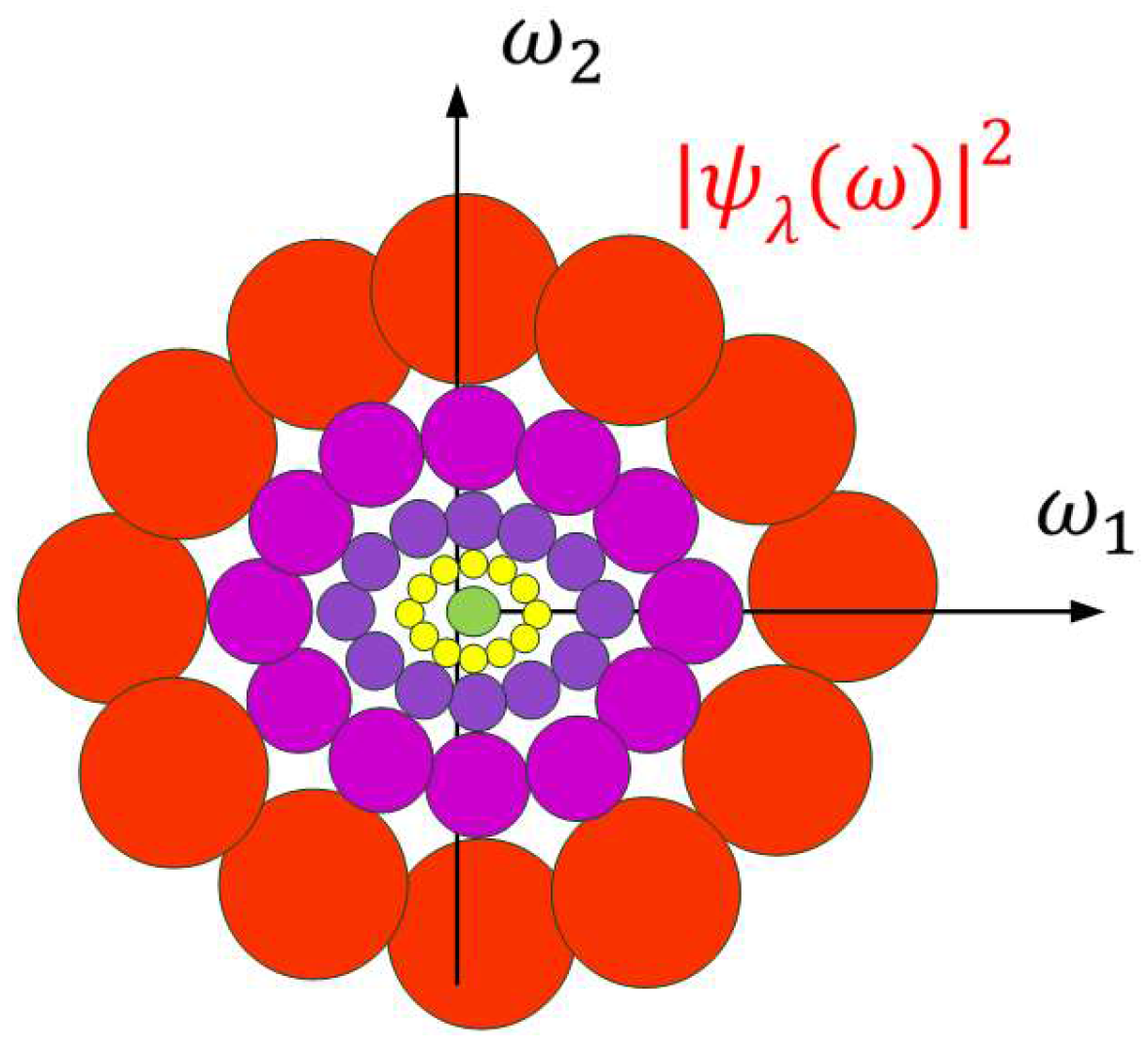
If the Fourier transform is centered at a frequency , then , which is centered at with its bandwidth proportional to . The Fourier transform is shown in Figure 1.
Wavelet transform is a mapping of local information, which represents the local features of the image, but the convolution operation is covariant to translations. Therefore, these local features are not translational invariant. To build a translational invariant representation, it is necessary to introduce a nonlinearity M. After this nonlinear transformation, , should be stable for deformation. At the same time, the nonlinear transformation operator M must be nonexpansive, so as to ensure the stability to additive noise. While satisfying the above conditions, it is also necessary to retain the energy information of the signal, resulting the translational invariant coefficients are then norms:
The norms are a rough signal representation, which show the sparsity of wavelet coefficients. Although the process of performing a modulus will lose phase information of the wavelet transform, but the loss of information is not from this process. It has been proved that x can be reconstructed from the modulus of its wavelet coefficients [17]. The loss of information actually comes from the integration of . This process removes all nonzero frequencies and then recovered when calculating the wavelet coefficients of . The norms of λ1 and λ2 define a deeper representation of the translational invariance:
By further iterating on the wavelet transform and modulus operators, more translational invariant coefficients can be computed. Let , along a path sequence , an ordered product of nonlinear and noncommuting operators is computed:
with . The scattering transformation along path p is defined as follows:
The scattering coefficient has translational invariance for x. It can be seen from Equation (6) that the transform has many similarities with the Fourier transform modulus, but the wavelet scattering coefficients have Lipschitz continuity for the deformation, as opposed to the Fourier transform modulus.
In terms of classification, the extracted local features are usually described as having translational invariance when the scale is less than the predefined scale 2J, while maintaining a spatial variability when the scale is greater than 2J. This requires a spatial window to localize the scattering integral, thus defining a windowed scattering transform:
And hence
with . The convolution process with is essentially an average down-sampling process at a scale of 2J. The windowed scattering operator has local translational invariance and is stable to deformation.
This paper uses Morlet wavelet as an example of complex wavelets, which is given by
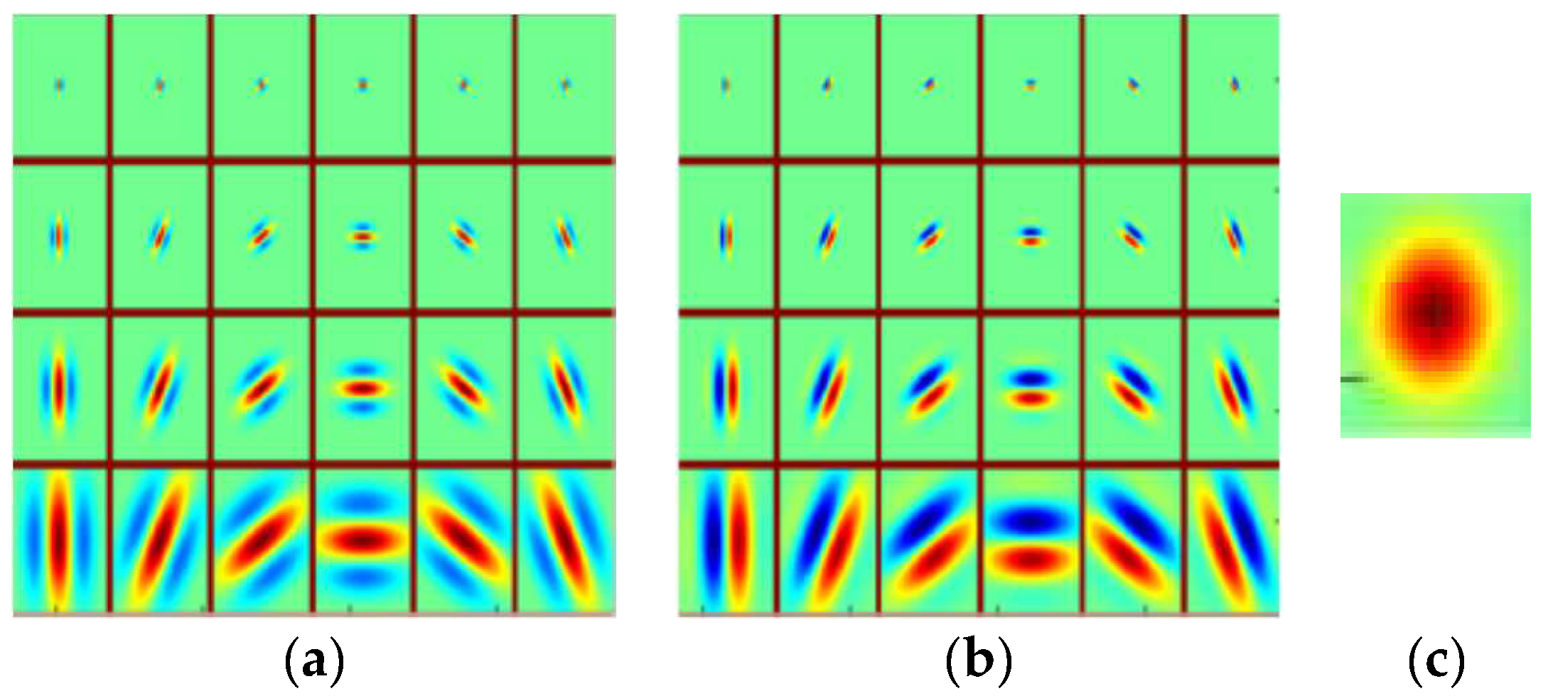
where is adjusted so that . The averaging filter is a scaled Gaussian. Figure 2 shows the Morlet wavelet with σ = 0.85 and ξ = 3π/4.
2.2. Scattering Convolution Network
If is a path of length m, then is the m-order windowing scattering coefficient, calculated at the m-th layer of the network. By further iterating on wavelet transform and modulus operators, scattering transform can compute higher order coefficients. Images are real-valued signals, so it is sufficient to consider “positive” rotations with angles in [0, π]:
with . It should be noted that 2J and 2j are spatial scale variables, while is a frequency index giving the location of the frequency support of . So that the following wavelet modulus propagator can be obtained:
A wavelet modulus propagator keeps the low-frequency averaging and computes the modulus of complex wavelet coefficients. High frequency information is lost because of an average pooling, but can be recovered at the next layer as the wavelet coefficients [9]. Therefore, it is important to build a multilayer network structure. Iterating on can construct a multilayer wavelet-scattering convolution network. This process can be illustrated as applying to all propagated signals of the m-th layer Pm, and the network will output all scattering signals and compute all propagated signals on the next layer Pm+1:
The wavelet-scattering convolution network is very different from the conventional convolution network. Conventional convolution network outputs the results only on the last layer, and the parameters of the filter banks need to be learned from a large number of data samples, while the scattering coefficients of the wavelet-scattering convolution network are distributed at each layer, and the parameters of the filter banks are pre-defined [18,19]. The wavelet-scattering convolution network only needs to learn the parameters of the final supervised classifier. The related literature has shown that the energy of the scattering convolution network is concentrated in a few paths, and will approach zero as the path increases. In addition, first three layers of the scattering convolution network concentrate most of the image energy [20]. When m = 3, the structure of the scattering convolution network is shown in Figure 3. The downward arrow is the process of scattering propagation, and the upward arrow outputs the extracted scattering coefficients.
Approximating the scattering process by a cosine basis along the scale and rotation variables, paths can be parameterized by .
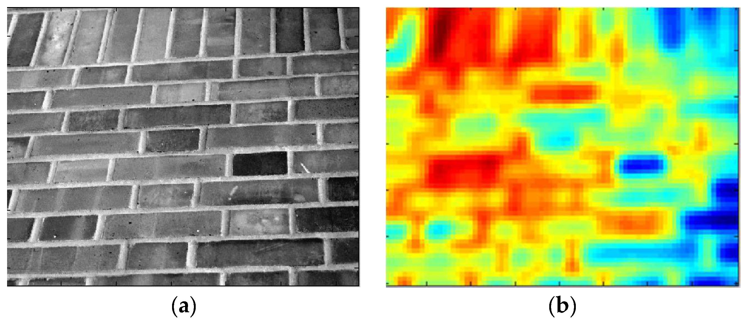
The following is an example of a texture image, which is used to explain the wavelet scattering network. The input signal in the example is a 2-D texture picture, as shown in Figure 4a. On layer 0, the scattering coefficients is , as shown in Figure 4b. Scattering coefficients outputted on layer 1 and layer 2 are also shown in Figure 5 and Figure 6 respectively.
In this example, J = 5, L = 6. The scaling factor of the wavelet function satisfies , , the rotation angle .
The final output of the wavelet-scattering convolution network is useful for classification, and can be expressed as:
Mallat et al. has shown in the literature [15] that the wavelet scattering coefficients have the following properties:
- Preservation of energy: ;
- Stable to additive noise: ;
- Translation covariance: the wavelet scattering coefficients will translate the same distance with the signal: ;
- Local translation invariance: ;
- Sensitive to rotation: ;
- Stable to slight deformation: ;
The scattering coefficient is insensitive to local translation, noise, and slight deformation, eliminating some of the factors that cause interference to the signal classification. In summary, the wavelet scattering coefficient is a good choice of feature representation, which requires no training but preserve a hierarchical structure.
2.3. Deep Roto-Translation Scattering Network
The wavelet coefficients in the previous subsection only satisfy the local translation invariance, but cannot reduce the interference caused by the rotation change on the signal classification. The wavelet-scattering convolution network (WSCN) can flexibly set the wavelet basis function so that the final output is insensitive to rotation changes. In 2015, Mallat proposed a deep roto-translation scattering network [16], which was insensitive to both local translation and rotation changes. The main idea is that for a two-layer wavelet scattering network, the first layer calculates a 2-D wavelet transform along the spatial variable to realize local translation invariance:
The second layer calculates a 3-D wavelet transform along both the spatial variable and the angle variable θ to realize local rotation invariance:
The specific process is described in detail as follows:
For the first layer of the wavelet-scattering convolution network, the wavelet function is the rotation and scale transform of band-pass filter Ψ:
The Morlet wavelet is still chosen here. The original input signal is computed convolution and modulus with , and then subsampled at intervals of , where .
The intermediate result for the first layer of the network is:
For the second layer of the wavelet-scattering convolution network, a 3-D wavelet function is selected:
where , β is the rotation angle parameter, is a 1-D wavelet function with the variable θ, and its scale is 2k(1 ≤ k ≤ K < log2 L).
For any , the intermediate result is computed convolution and modulus with the 3-D wavelet function along the spatial variable u and the rotation angle variable θ, and then subsampled along both variables. The final intermediate result for the second layer is:
The final output is achieved by averaging the input x, the first layer intermediate result , and the second intermediate result with a spatial convolution with :
The wavelet scattering coefficients at this time have local translation and rotation invariance, and are not sensitive to perturbations and slight deformations. reduces the adverse effects of the rotation change on the signal classification, and helps to improve the accuracy of complex signal classification.
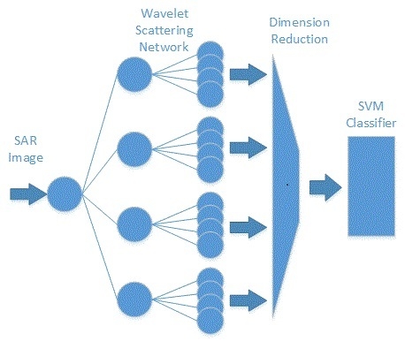
This paper then trains the Gaussian kernel support vector machine using the wavelet scattering coefficients to realize SAR image automatic target recognition. The overall architecture is depicted in Figure 7.
3. Experiments on the MSTAR benchmark dataset
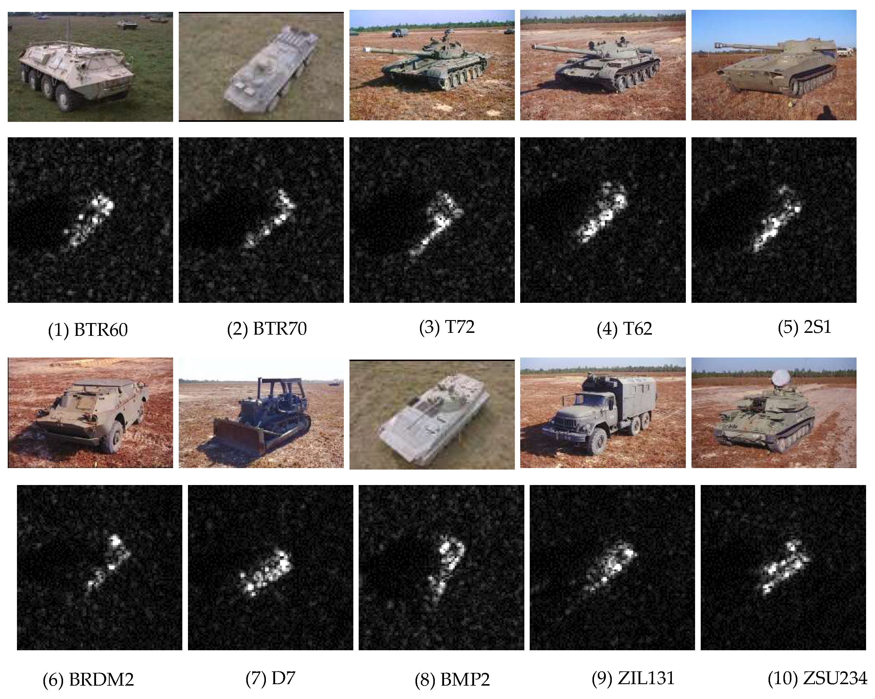
The experimental data used in this paper were collected by Sandia National Laboratory (SNL) SAR sensors. The data were collected under the moving and stationary target acquisition and recognition (MSTAR) project [4], which was jointly sponsored by Defense Advanced Research Projects Agency (DARPA) and Air Force Research Laboratory (AFRL). The project collected hundreds of thousands of SAR images containing ground military targets, including different target classes, aspect and depression angles, barrel steering, configuration changes and variants, but only a small portion of which can be available on the website for the open access [21]. The released MSTAR data set contains 10 classes of ground military targets listed in Table 1. These images are collected by the X-band SAR sensor in a 0.3 m resolution spotlight mode; full aspect coverage (range from 0° to 360°), with a relative flat grass or exposed soil background. It should be also noticed that the released data were all stationary targets. Figure 8 shows the optical images of 10 classes of military targets and the corresponding SAR images at the same aspect angle.
The algorithm is tested under both standard operating conditions (SOC) and extended operating conditions (EOC) in order to completely assess the robustness of the method. The standard operating conditions refer to the configuration and serial number of the training and testing SAR images are the same, but the depression and aspect angle for the images are different. The extended operating conditions refer to the significant differences between the training and testing SAR images, which is mainly due to the great change of the depression angle and configuration, as well as version variants. Configuration changes mean the addition or removal of discrete components on the target, such as auxiliary fuel barrel changes.
3.1. SOC Results
Under standard operating conditions, the method is tested for the classification of 10 classes. The serial number of the training and test set, the depression angle, and the number of samples for each class are shown in Table 2. The same target class has the same serial number in the training set and the test set, but the depression and aspect angle are different. The training SAR images are collected at 17° depression angle, while the test SAR images are collected at 15° depression angle. No image preprocessing algorithm is applied to the SAR images. Table 3 shows the correct classification coefficient and confusion matrix for the classification of 10 classes of targets under SOC. Each row in the confusion matrix represents the actual target class, and each column denotes the class predicted by the network. Percent Correctly Classified () is used to assess the performance of the ATR, which is defined as , where the is the number of correct classified positive samples, and the is the total number of samples. It can be seen that the proposed method can achieve state-of-the-art performance for the classification of MSTAR 10 classes of targets under standard operating conditions. The proposed method achieves an overall accuracy of 97.63% for the SOC dataset. The kappa coefficient is 0.97, which indicates this method is stable for 10 classes of targets. Correct classification coefficients are all over 96%, except target 2S1, a part of which was misclassified as T-62 and BTR-70. From the images shown in Figure 8, structure of T-62 and 2S1 is similar; further, barrel part is hardly seen in SAR images, thus SAR images of 2S1 and BTR-70 are also similar.
3.2. EOC Results
A SAR image is quite sensitive to the change of depression angle, and even a slight change will result in a very different image. As shown in Table 4, only four classes of targets in the MSTAR data set contain SAR images at a 30° depression angle and they are 2S1, BRDM-2, T-72, and ZSU-234. Therefore, SAR images with these four classes of targets at a 17° depression angle are used for training, and those at 30° depression angle are used for testing. The correct classification coefficient and confusion matrix for the significant change of depression angle denoted as EOC-1 are shown in Table 5. The overall accuracy is 82.46% under EOC-1, and its kappa coefficient is 0.766. As we all know that SAR is sensitive to incidence angle, which EOC-1 means significant variance of depression angle. Therefore, the feature of SAR image changes, which leads to the degradation of correct classification coefficient.
The extended operating conditions also include configuration variants and version variants. Configuration variants mainly refer to whether both sides of the tank track have the installation of protective plate, or whether the tank tail is installed with fuel barrels, as well as the rotation of the turrets and the barrels, while version variants refer to different versions, denoted as EOC-2. The algorithm is tested under this condition to evaluate the classification performance. SAR images of the four classes of targets, namely BMP-2, BRDM-2, BTR-70, and T-72, at a 17° depression angle are used as training set as shown in Table 2. Two version variants of BMP-2 and ten version variants of T-72 collected at 17° and 15° depression angles are listed in Table 6 and Table 7, respectively, as two groups of test sets. It is worth mentioning that the training set does not include the serial number of the test set. The correct classification coefficient and confusion matrix are listed in Table 8 and Table 9. WSCN shows its stable performance for the configuration variants of T-72 and BMP-2. The correct classification coefficient is obtained at 94.14% for five version variants T-72, and 89.76% for five versions T-72 and two version variants BMP-2.
It can be seen that the significant change of depression angle has a great influence on the classification result. Details of the EOC-1 data are shown in Table 10, and the correct classification coefficient and confusion matrix using 10-class targets to train the network and 4-class to test are shown in Table 11. Due to the large difference of the train and test data, the accuracy decreases to 74.37% from the 82.46% of the original EOC-1 experiment. As showing in the Table 11, some ZSU-234 are classified to D7 and leading to lower accuracy.
4. Discussion
The performance of WSCN is compared with several widely cited methods and recently proposed methods, as well as our previous work [1] in Table 12. The methods include conditional Gaussian model (Cond Gauss) [22], monogenic scale space (MSS) [23], and modified polar mapping classifier (M-PMC) [24], and information-decoupled representation (IDR) [25]. Note that the testing samples used in MSS and IDR under EOC-1 only contains three classes, but ours contains four classes. While the testing samples used in M-MPC under EOC-2 contains the samples with the depression angle both 15 and 17 degrees. The classification performance of A-ConvNets [1] is slightly better. It is reasonable because A-ConvNets is regarded a fully trainable network including the feature extraction part, while our approach employs a fixed feature extraction network. There are some inherent shortcomings for fully-trainable approaches such as A-ConvNet. Firstly, a large number of training samples are needed to avoid overfitting. Secondly, there are many hyper parameters needed to be optimized through multiple times of manual trial. Finally, deep neural network as blackbox is known to be difficult to understand and diagnose, as the parameters are often initialized randomly and then optimized only depending on the train samples, the network’s procedure and final state is unknown and unpredictable. While the proposed WSCN is fully based on rational design backed by mathematical theory. In these regards, the proposed WSCN is preferable albeit it’s slightly worse performance. An additional experiment of A-ConvNets is conducted on the same dataset of the WSCN, The results indicate that WSCN can efficiently recognize the target with configuration changes, but sensitive to the angles. As opposed to deep neural networks, filters of each layer in wavelet-scattering convolution network are predefined except the final supervised classifier. Therefore, the parameters needed to be learned from the training samples are greatly reduced, thus reducing the probability of overfitting and the number of training samples. Moreover, the number of tests is reduced because the hyper parameters that require manual adjustment are very limited. In addition, mathematical theory can prove that by constructing a specific wavelet function, the output scattering coefficients of wavelet-scattering convolution network can be invariant to local translation and rotation, as well as insensitive to perturbation and slight deformation.
5. Conclusions
This paper presents a SAR automatic target classification method based on a wavelet-scattering convolution network. By introducing a deep roto-translation scattering network with complex wavelet filters over spatial and angular variables, robust feature representations can be extracted across multiple scales and multiple angles. Parameters of WSCN are predefined rather than randomly initialized parameters as deep neural network. It does not require any training samples. CNN is trained with the back-propagation algorithm, which optimizes the parameters according to the train samples, thus the parameters end up at an unknown and unpredictable state, and the optimization is uncontrollable which only depends on the input samples for each train step. Unlike CNN, the design of the WSCN is purely based on the priori knowledge and mathematical principles. The proposed algorithm was verified on MSTAR benchmark dataset under both SOC and EOC cases. Experimental results show that 97.63% accuracy was obtain in SOC, and 82.46% for significant change of depression angle from 17° to 30°, and 94.14% for configuration variants of T-72 tank, and 89.76% for version variants of T-72 and BMP-2. The proposed method shows robustness on the variants of configuration, and acceptable accuracy on significant variance of depression angle. Experimental results indicate the proposed method can yield comparable results with state-of-the-art deep neural network method which, on the other hand, requires a significant amount of training samples. In this paper, the training samples of proposed WSCN are less than 1/10 of those in previous A-ConvNets.
The time consumption of proposed method mainly includes three parts: the features extraction, the features dimension reduction and classification. The experiments are conducted by MATLAB 2015b in an Ubuntu 14.04 operation system. The computer has an Intel Core i7-5930K CPU and its memory is 128 G. The experiment under the SOC-1 can be finished in 23 min. The computing time is 0.062 s per image for scattering features extraction, and 0.207 s per image for dimension reduction. The classification of whole 2425 test images only costs 0.172 s. It should be noticed the classifier can be trained offline, which could significantly reduce the time cost. Furthermore, in this paper, the roto-translation of SAR images and the feature dimension reduction are carried out by MATLAB code, which could be further optimized by other high efficient program languages.
Acknowledgments
This work was supported by the Natural Science Foundation of China, grant No. 61571132, 61571134 and 61331020.
Author Contributions
H.W. conceived and designed the study and wrote the paper; S.L., Y.Z. and S.C. conducted the study.
Conflicts of Interest
The authors declare no conflicts of interest.
References
- Chen, S.; Wang, H.; Xu, F.; Jin, Y. Target Classification Using the Deep Convolutional Networks for SAR Images. IEEE Trans. Geosci. Remote Sens. 2016, 54, 4806–4817. [Google Scholar] [CrossRef]
- Dudgeon, D.E.; Lacoss, R.T. An Overview of Automatic Target Recognition. Linc. Lab. J. 1993, 6, 3–10. [Google Scholar]
- Novak, L.M.; Owirka, G.J.; Brower, W.S.; Weaver, A.L. The Automatic Target Recognition System in SAIP. Linc. Lab. J. 1997, 10, 187–201. [Google Scholar]
- Keydel, E.R.; Lee, S.W.; Moore, J.T. MSTAR extended operating conditions: A tutorial. Int. Soc. Opt. Photonics 1996. [Google Scholar] [CrossRef]
- Kaplan, L.M. Improved SAR target detection via extended fractal features. IEEE Trans. Aerosp. Electron. Syst. 2001, 37, 436–451. [Google Scholar] [CrossRef]
- Zhao, Q.; Principe, J.C. Support vector machines for SAR automatic target recognition. IEEE Trans. Aerosp. Electron. Syst. 2001, 37, 643–654. [Google Scholar] [CrossRef]
- Sun, Y.; Liu, Z.; Todorovic, S.; Li, J. Adaptive boosting for SAR automatic target recognition. IEEE Trans. Aerosp. Electron. Syst. 2007, 43, 112–125. [Google Scholar] [CrossRef]
- Huang, Z.; Pan, Z.; Lei, B. Transfer Learning with Deep Convolutional Neural Network for SAR Target Classification with Limited Labeled Data. Remote Sens. 2017, 9, 907. [Google Scholar] [CrossRef]
- Hinton, G.E.; Salakhutdinov, R.R. Reducing the dimensionality of data with neural networks. Science 2006, 313, 504–507. [Google Scholar] [CrossRef] [PubMed]
- Zhu, X.X.; Tuia, D.; Mou, L.; Xia, G.; Zhang, L.; Xu, F.; Fraundorfer, F. Deep Learning in Remote Sensing: A Comprehensive Review and List of Resources. IEEE Geosci. Remote Sens. Mag. 2018, 5, 8–36. [Google Scholar] [CrossRef]
- Liu, Z.Y.; Liu, B.; Guo, W.W.; Zhang, Z.H.; Zhang, B.; Zhou, Y.H.; Gao, M.; Yu, W.X. Ship Detection in GF-3 NSC Mode SAR Images. J. Radars. 2017, 6, 473–482. [Google Scholar]
- Song, S.; Xu, B.; Yang, J. SAR Target Recognition via Supervised Discriminative Dictionary Learning and Sparse Representation of the SAR-HOG Feature. Remote Sens. 2016, 8, 683. [Google Scholar] [CrossRef]
- Dou, F.; Diao, W.; Sun, X.; Zhang, Y.; Fu, K. Aircraft Reconstruction in High-Resolution SAR Images Using Deep Shape Prior. ISPRS Int. J. Geo-Inf. 2017, 6, 330. [Google Scholar] [CrossRef]
- Mallat, S. Group invariant scattering. Commun. Pure Appl. Math. 2012, 65, 1331–1398. [Google Scholar] [CrossRef]
- Bruna, J.; Mallat, S. Invariant scattering convolution networks. IEEE Trans. Pattern Anal. Mach. Intell. 2013, 35, 1872–1886. [Google Scholar] [CrossRef] [PubMed]
- Oyallon, E.; Mallat, S. Deep roto-translation scattering for object classification. In Proceedings of the 2015 IEEE Conference on Computer Vision and Pattern Recognition (CVPR), Boston, MA, USA, 7–12 June 2015. [Google Scholar]
- Waldspurger, I.; d’Aspremont, A.; Mallat, S. Phase recovery, maxcut and complex semidefinite programming. Math. Program. 2015, 149, 47–81. [Google Scholar] [CrossRef]
- Sifre, L.; Mallat, S. Combined scattering for rotation invariant texture analysis. In Proceedings of the 2012 European Symposium on Artificial Neural Networks, Computational Intelligence and Machine Learning, Bruges, Belgium, 25–27 April 2012. [Google Scholar]
- Bruna, J. Scattering Representations for Recognition. Ph.D. Thesis, École Polytechnique, Palaiseau, France, 2013. [Google Scholar]
- Sifre, L.; Mallat, S. Rotation, scaling and deformation invariant scattering for texture discrimination. In Proceedings of the 2013 IEEE Conference on Computer Vision and Pattern Recognition, Portland, OR, USA, 23–28 June 2013. [Google Scholar]
- The Air Force Moving and Stationary Target Recognition Database. Available online: https://www.sdms.afrl.af.mil/datasets/mstar/ (accessed on 28 October 2013).
- O’Sullivan, J.A.; DeVore, M.D.; Kedia, V.; Miller, M.I. SAR ATR performance using a conditionally Gaussian model. IEEE Trans. Aerosp. Electron. Syst. 2001, 37, 91–108. [Google Scholar] [CrossRef]
- Dong, G.; Kuang, G. Classification on the monogenic scale space: Application to target recognition in SAR image. IEEE Trans. Image Process. 2015, 24, 2527–2539. [Google Scholar] [CrossRef] [PubMed]
- Park, J.I.; Kim, K.T. Modified Polar Mapping Classifier for SAR Automatic Target Recognition. IEEE Trans. Aerosp. Electron. Syst. 2014, 50, 1092–1107. [Google Scholar] [CrossRef]
- Ming, C.; Xuqun, Y. Target Recognition in SAR Images Based on Information-Decoupled Representation. Remote Sens. 2018, 10, 138. [Google Scholar] [CrossRef]
Figure 1.
Fourier transform of .

Figure 2.
(a) The real part of Morlet wavelet; (b) the imaginary part of Morlet wavelet; (c) Gaussian function, where scale changes are arranged in rows, 1 ≤ j ≤ 4, and rotation changes are arranged in columns, L = 8.
Figure 2.
(a) The real part of Morlet wavelet; (b) the imaginary part of Morlet wavelet; (c) Gaussian function, where scale changes are arranged in rows, 1 ≤ j ≤ 4, and rotation changes are arranged in columns, L = 8.

Figure 3.
Scattering convolution network diagram.
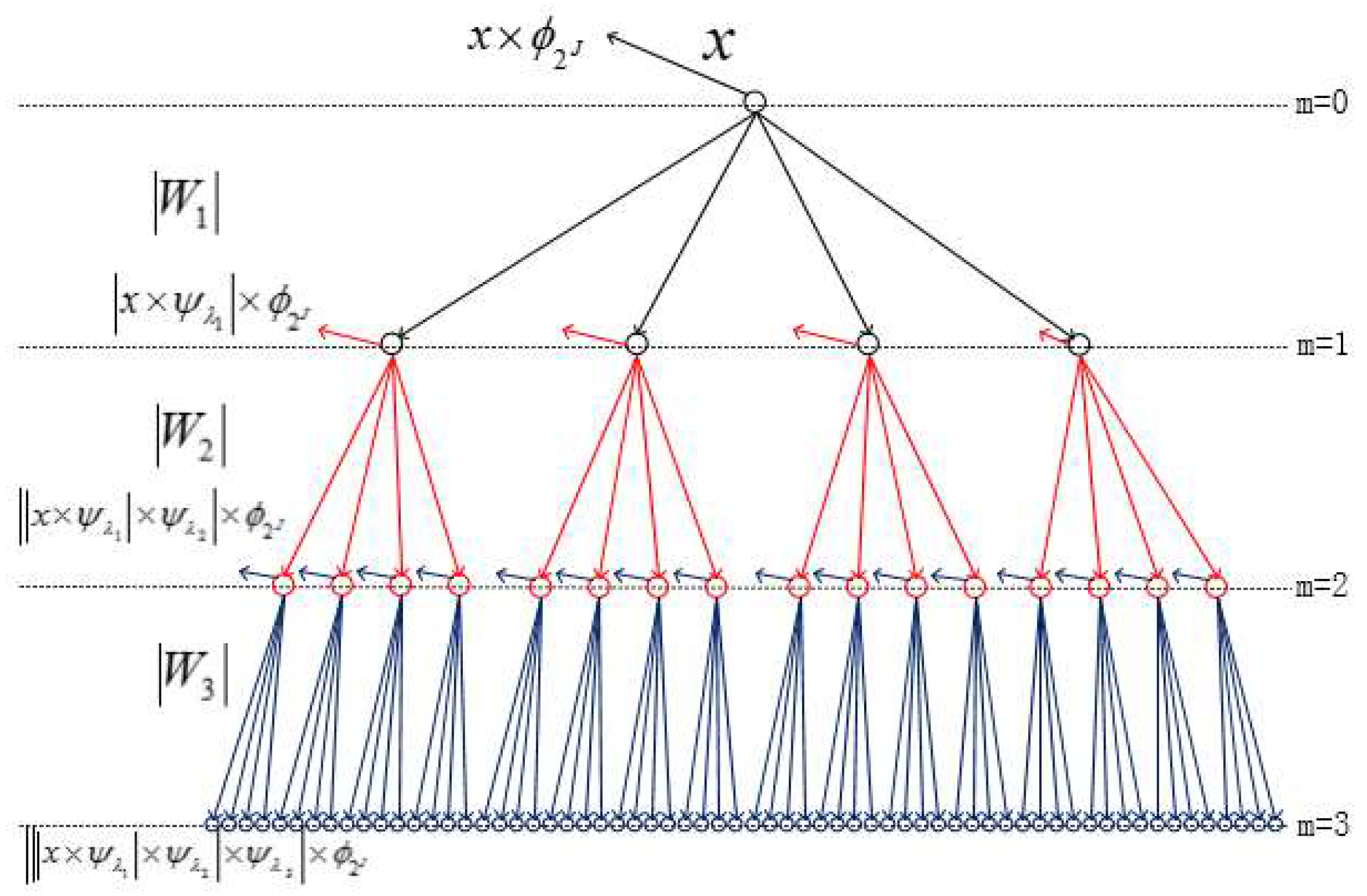
Figure 4.
(a) Input of a 2-D texture image; (b) output scattering coefficients , on layer-0.

Figure 5.
Output scattering coefficients , on layer 1, where scale changes are arranged in rows, and the rotation changes are arranged in columns.
Figure 5.
Output scattering coefficients , on layer 1, where scale changes are arranged in rows, and the rotation changes are arranged in columns.
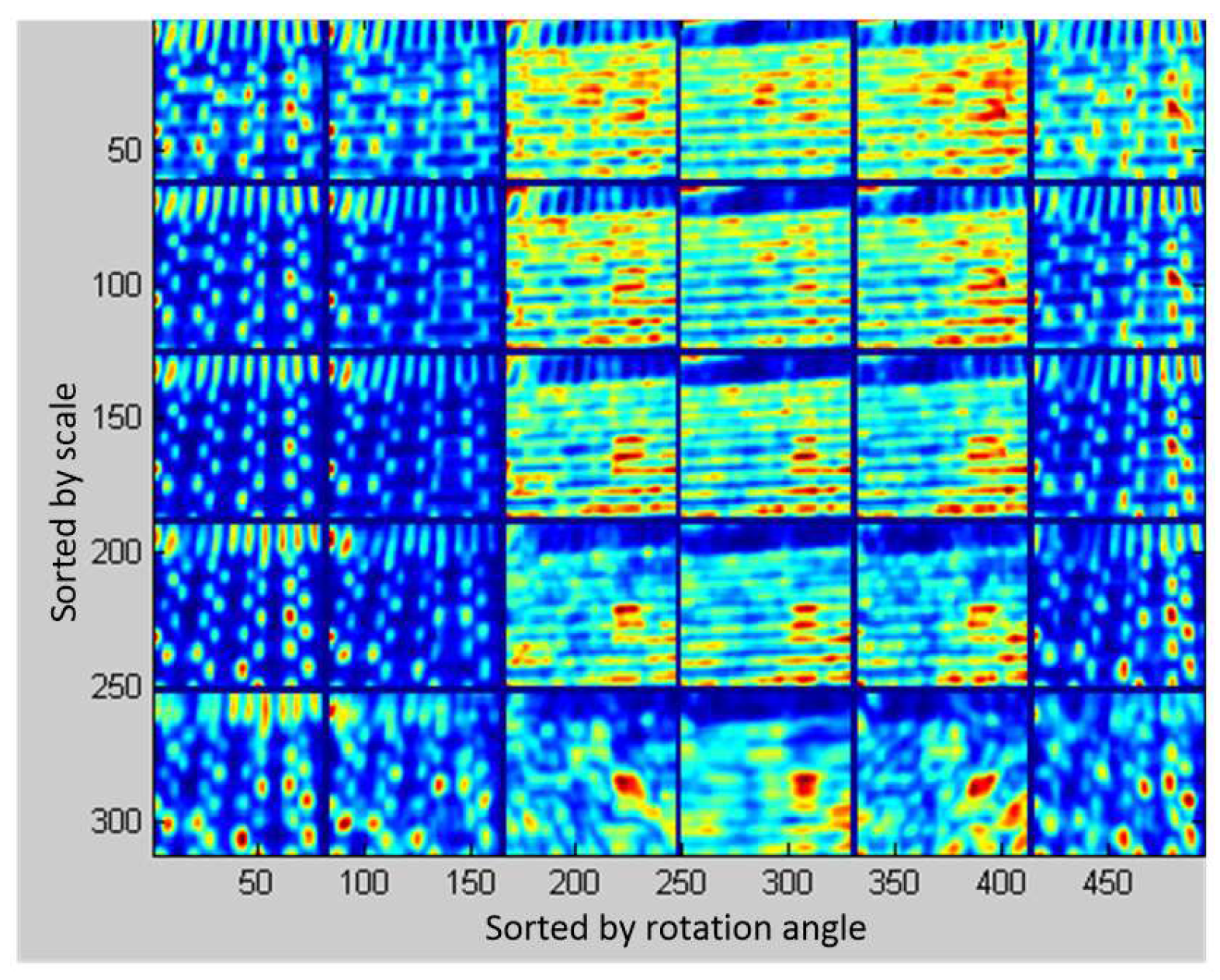
Figure 6.
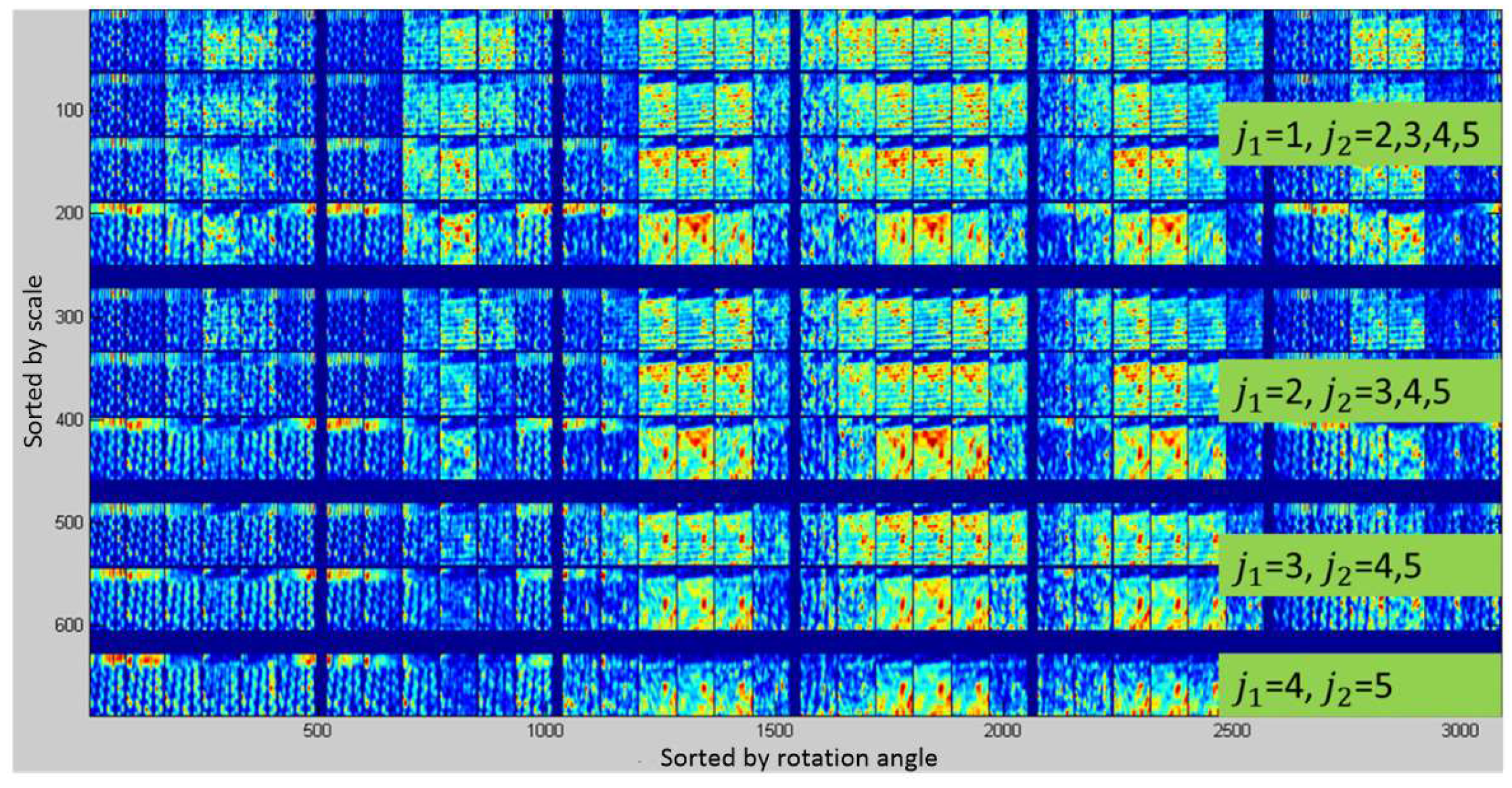
Output scattering coefficients on layer 2, where scale changes are arranged in rows, and the rotation changes are arranged in columns.
Figure 6.
Output scattering coefficients on layer 2, where scale changes are arranged in rows, and the rotation changes are arranged in columns.

Figure 7.
Architecture of the proposed approach.
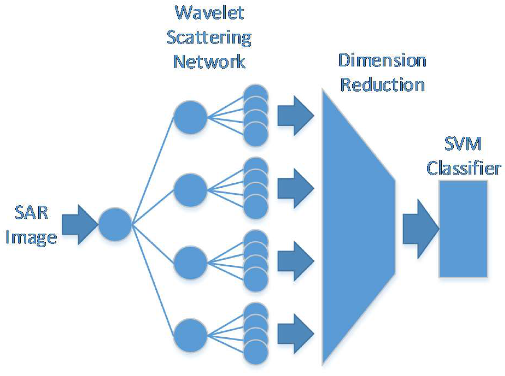
Figure 8.
Examples of 10 classes of military targets: optical image (Top) and SAR image (Bottom).

Table 1.
Ten classes of ground military targets.
| Targets | Classes |
|---|---|
| Armored personnel carrier | BMP-2, BRDM-2, BTR-60, BTR-70 |
| Tank | T-62, T-72 |
| Rocket launcher | 2S1 |
| Air defense unit | ZSU-234 |
| Truck | ZIL-131 |
| Bulldozer | D7 |
Table 2.
Statistical data for training and testing SAR images under SOC.
| Class | Serial No. | Train | Test | ||
|---|---|---|---|---|---|
| Depression | No. Images | Depression | No. Images | ||
| BMP-2 | 9563 | 17° | 233 | 15° | 195 |
| BTR-70 | c71 | 17° | 233 | 15° | 196 |
| T-72 | 132 | 17° | 232 | 15° | 196 |
| BTR-60 | k10yt7532 | 17° | 256 | 15° | 195 |
| 2S1 | b01 | 17° | 299 | 15° | 274 |
| BRDM-2 | E-71 | 17° | 298 | 15° | 274 |
| D7 | 92v13015 | 17° | 299 | 15° | 274 |
| T-62 | A51 | 17° | 299 | 15° | 273 |
| ZIL-131 | E12 | 17° | 299 | 15° | 274 |
| ZSU-234 | d08 | 17° | 299 | 15° | 274 |
Table 3.
Accuracy and confusion matrix under SOC.
| BMP-2 | BRDM-2 | BTR-60 | BTR-70 | D7 | 2S1 | T-62 | T-72 | ZIL-131 | ZSU-234 | Pcc (%) | |
|---|---|---|---|---|---|---|---|---|---|---|---|
| BMP-2 | 190 | 2 | 0 | 1 | 0 | 1 | 0 | 1 | 0 | 0 | 97.4 |
| BRDM-2 | 0 | 272 | 0 | 0 | 0 | 0 | 0 | 0 | 2 | 0 | 99.3 |
| BTR-60 | 0 | 0 | 189 | 3 | 0 | 0 | 0 | 0 | 2 | 1 | 96.9 |
| BTR-70 | 0 | 0 | 0 | 196 | 0 | 0 | 0 | 0 | 0 | 0 | 100 |
| D-7 | 0 | 0 | 0 | 0 | 272 | 0 | 0 | 0 | 2 | 0 | 99.3 |
| 2S1 | 4 | 1 | 2 | 9 | 0 | 239 | 9 | 0 | 7 | 3 | 87.2 |
| T-62 | 1 | 0 | 0 | 1 | 0 | 0 | 264 | 2 | 0 | 5 | 96.7 |
| T-72 | 0 | 0 | 0 | 0 | 0 | 1 | 0 | 195 | 0 | 0 | 99.5 |
| ZIL-131 | 0 | 0 | 0 | 0 | 0 | 0 | 0 | 0 | 274 | 0 | 100 |
| ZSU-234 | 0 | 0 | 0 | 0 | 0 | 0 | 0 | 0 | 0 | 274 | 100 |
| Total | 97.63 | ||||||||||
Table 4.
Statistical data for training and testing SAR images under EOC-1.
| Class | Serial No. | Train | Test | ||
|---|---|---|---|---|---|
| Depression | No. Images | Depression | No. Images | ||
| 2S1 | b01 | 17° | 299 | 30° | 288 |
| BRDM-2 | E-71 | 17° | 298 | 30° | 287 |
| T-72 | A64 | 17° | 299 | 30° | 288 |
| ZSU-234 | d08 | 17° | 299 | 30° | 288 |
Table 5.
Accuracy and confusion matrix under EOC-1 (significant change of depression angle).
| 2S1 | BRDM-2 | T-72 | ZSU-234 | Pcc (%) | |
|---|---|---|---|---|---|
| 2S1 | 205 | 50 | 33 | 0 | 71.18 |
| BRDM-2 | 7 | 270 | 8 | 2 | 94.08 |
| T-72 | 39 | 20 | 202 | 27 | 70.14 |
| ZSU-234 | 3 | 4 | 9 | 272 | 94.44 |
| Total | 82.46 | ||||
Table 6.
Statistical data for training and testing SAR images under EOC-2 (configuration variants).
| Class | Serial No. | Depression | No. Images |
|---|---|---|---|
| T-72 | S7 | 15°, 17° | 419 |
| A32 | 15°, 17° | 572 | |
| A62 | 15°, 17° | 573 | |
| A63 | 15°, 17° | 573 | |
| A64 | 15°, 17° | 573 |
Table 7.
Statistical data for training and testing SAR images under EOC-2 (version variants).
| Class | Serial No. | Depression | No. Images |
|---|---|---|---|
| BMP-2 | 9566 | 15°, 17° | 428 |
| c21 | 15°, 17° | 429 | |
| T-72 | 812 | 15°, 17° | 426 |
| A04 | 15°, 17° | 573 | |
| A05 | 15°, 17° | 573 | |
| A07 | 15°, 17° | 573 | |
| A10 | 15°, 17° | 567 |
Table 8.
Accuracy and confusion matrix under EOC-2 (configuration variants).
| Serial No. | BMP-2 | BRDM-2 | BTR-70 | T-72 | Pcc (%) | |
|---|---|---|---|---|---|---|
| T-72 | S7 | 8 | 0 | 8 | 403 | 96.18 |
| A32 | 24 | 7 | 0 | 541 | 94.58 | |
| A62 | 10 | 14 | 1 | 548 | 95.63 | |
| A63 | 5 | 17 | 9 | 542 | 94.59 | |
| A64 | 5 | 48 | 6 | 514 | 89.70 | |
| Total | 94.14 | |||||
Table 9.
Accuracy and confusion matrix under EOC-2 (version variants).
| Serial No. | BMP-2 | BRDM-2 | BTR-70 | T-72 | Pcc (%) | |
|---|---|---|---|---|---|---|
| BMP-2 | 9566 | 343 | 5 | 17 | 63 | 80.14 |
| c21 | 331 | 11 | 22 | 65 | 77.16 | |
| T-72 | 812 | 16 | 4 | 15 | 391 | 91.78 |
| A04 | 32 | 42 | 8 | 491 | 85.69 | |
| A05 | 2 | 8 | 0 | 563 | 98.25 | |
| A07 | 4 | 18 | 1 | 550 | 95.99 | |
| A10 | 0 | 3 | 1 | 563 | 99.29 | |
| Total | 89.76 | |||||
Table 10.
Statistical data for training and testing SAR images under additional EOC-1.
| Class | Serial No. | Train | Test | ||
|---|---|---|---|---|---|
| Depression | No. Images | Depression | No. Images | ||
| BMP-2 | 9563 | 17° | 233 | - | 0 |
| BTR-70 | c71 | 17° | 233 | - | 0 |
| T-72 | A64 | 17° | 299 | 30° | 288 |
| BTR-60 | k10yt7532 | 17° | 256 | - | 0 |
| 2S1 | b01 | 17° | 299 | 30° | 288 |
| BRDM-2 | E-71 | 17° | 298 | 30° | 287 |
| D7 | 92v13015 | 17° | 299 | - | 0 |
| T-62 | A51 | 17° | 299 | - | 0 |
| ZIL-131 | E12 | 17° | 299 | - | 0 |
| ZSU-234 | d08 | 17° | 299 | 30° | 288 |
Table 11.
Accuracy and confusion matrix under additional EOC-1 (significant change of depression angle).
Table 11.
Accuracy and confusion matrix under additional EOC-1 (significant change of depression angle).
| BMP-2 | BRDM-2 | BTR-60 | BTR-70 | D7 | 2S1 | T-62 | ZIL-131 | T-72 | ZSU-234 | Pcc (%) | |
|---|---|---|---|---|---|---|---|---|---|---|---|
| 2S1 | 1 | 28 | 0 | 0 | 6 | 229 | 1 | 0 | 23 | 0 | 79.51 |
| BRDM-2 | 0 | 271 | 0 | 0 | 1 | 11 | 0 | 0 | 4 | 0 | 94.42 |
| T-72 | 1 | 27 | 0 | 0 | 18 | 41 | 9 | 0 | 192 | 0 | 66.67 |
| ZSU-234 | 0 | 24 | 0 | 0 | 63 | 15 | 1 | 0 | 21 | 164 | 56.94 |
| Total | 74.37 | ||||||||||
Table 12.
Comparison with A-ConvNets.
| Method | SOC (%) | EOC-1 (%) | EOC-2 (%) | Training Samples |
|---|---|---|---|---|
| A-ConvNets [1] | 99.13 | 96.12 | 98.93 | 2700 per class |
| Cond Guass [22] | 98.9 | - | 79.3 | ~480 per class |
| MSS [23] | 96.6 | 98.2 | - | ~381 per class |
| M-PMC [24] | 98.8 | - | 97.3 | ~370 per class |
| IDR [25] | 94.9 | 99.0 | - | ~300 per class |
| A-ConvNets | 92.04 | 89.40 | 89.74 | ~230 per class |
| Our Method | 97.63 | 82.46 | 94.14 | ~230 per class |
© 2018 by the authors. Licensee MDPI, Basel, Switzerland. This article is an open access article distributed under the terms and conditions of the Creative Commons Attribution (CC BY) license (http://creativecommons.org/licenses/by/4.0/).
Share and Cite
MDPI and ACS Style
Wang, H.; Li, S.; Zhou, Y.; Chen, S. SAR Automatic Target Recognition Using a Roto-Translational Invariant Wavelet-Scattering Convolution Network. Remote Sens. 2018, 10, 501. https://doi.org/10.3390/rs10040501
AMA Style
Wang H, Li S, Zhou Y, Chen S. SAR Automatic Target Recognition Using a Roto-Translational Invariant Wavelet-Scattering Convolution Network. Remote Sensing. 2018; 10(4):501. https://doi.org/10.3390/rs10040501
Chicago/Turabian StyleWang, Haipeng, Suo Li, Yu Zhou, and Sizhe Chen. 2018. "SAR Automatic Target Recognition Using a Roto-Translational Invariant Wavelet-Scattering Convolution Network" Remote Sensing 10, no. 4: 501. https://doi.org/10.3390/rs10040501
Note that from the first issue of 2016, this journal uses article numbers instead of page numbers. See further details here.