Modeling Orbital Error in InSAR Interferogram Using Frequency and Spatial Domain Based Methods


Abstract
1. Introduction
2. Methods
2.1. Modeling Orbital Error in Frequency Domain
2.2. Modeling Orbital Error in Spatial Domain
2.2.1. Preprocess: Multi-Looking and Manually Masking
2.2.2. Polynomial Model
2.2.3. Iteratively Reweighted Least Squares Fitting
2.2.4. Model Selection
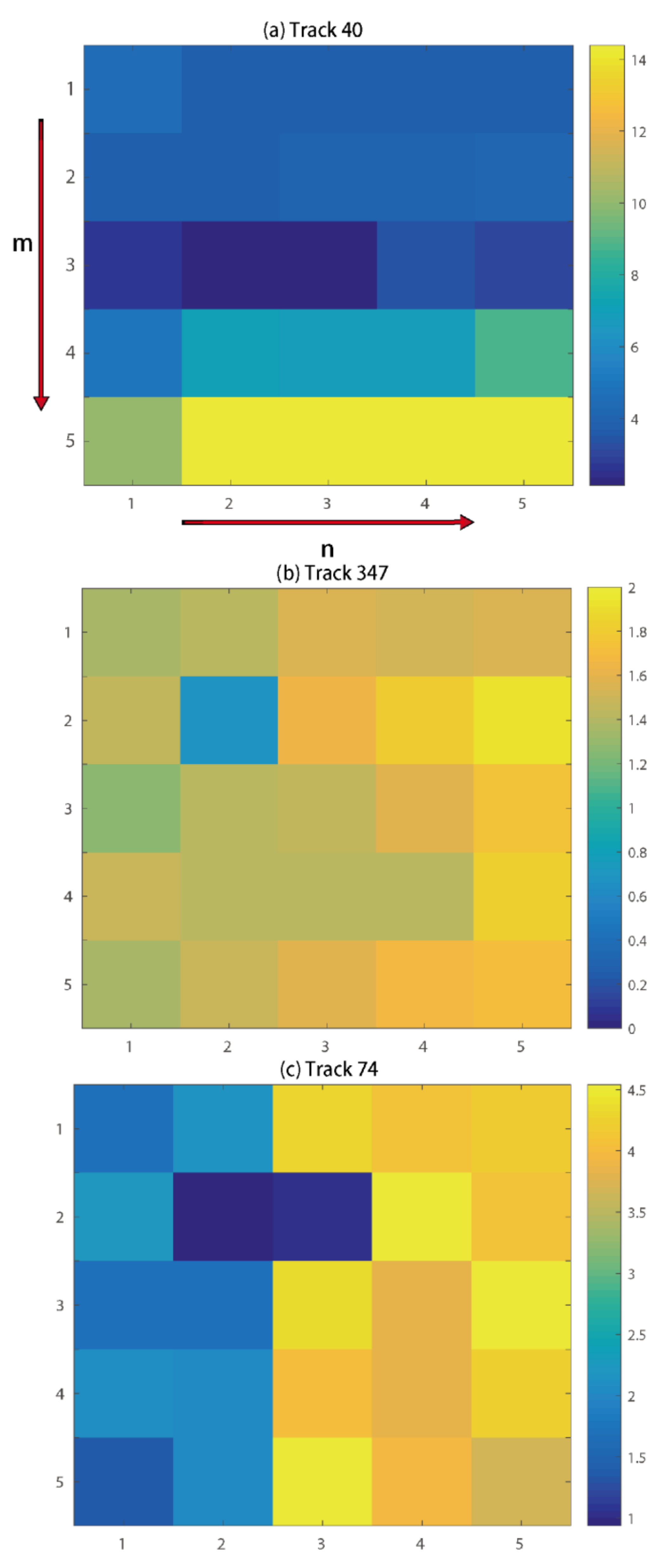
- Split data into subsamples with equivalent size .
- For , set validation data to be the subsample, and training data to be the other subsamples.
- Fit each model to and evaluate its performance on through weighted root-mean-square error (WRMSE).
- Pick and that leads to minimum WRMSE by averaging results.
3. Results
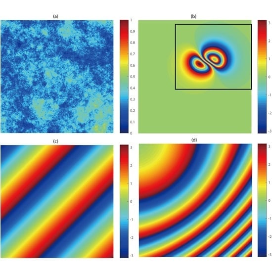
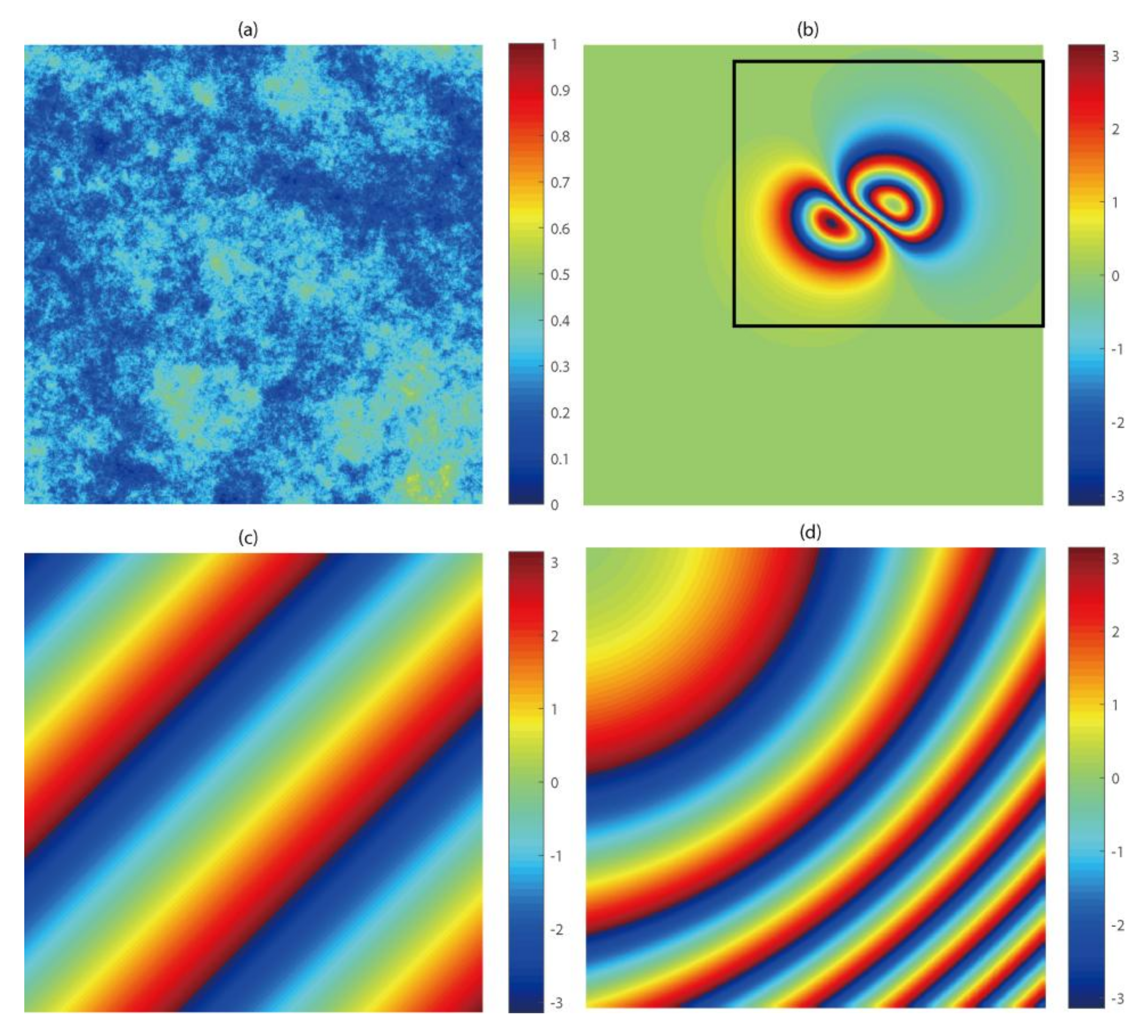
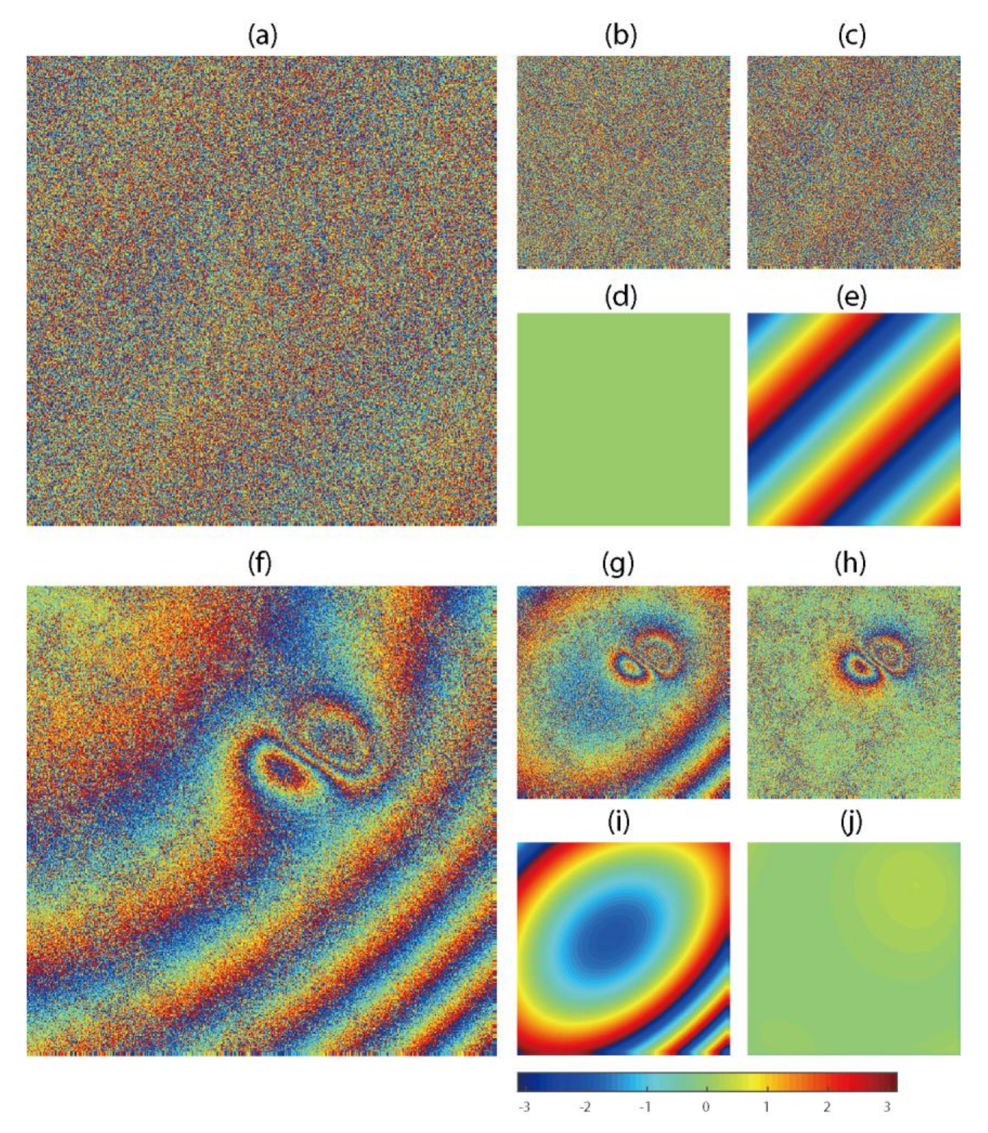
3.1. Synthetic Data
3.2. Real Data
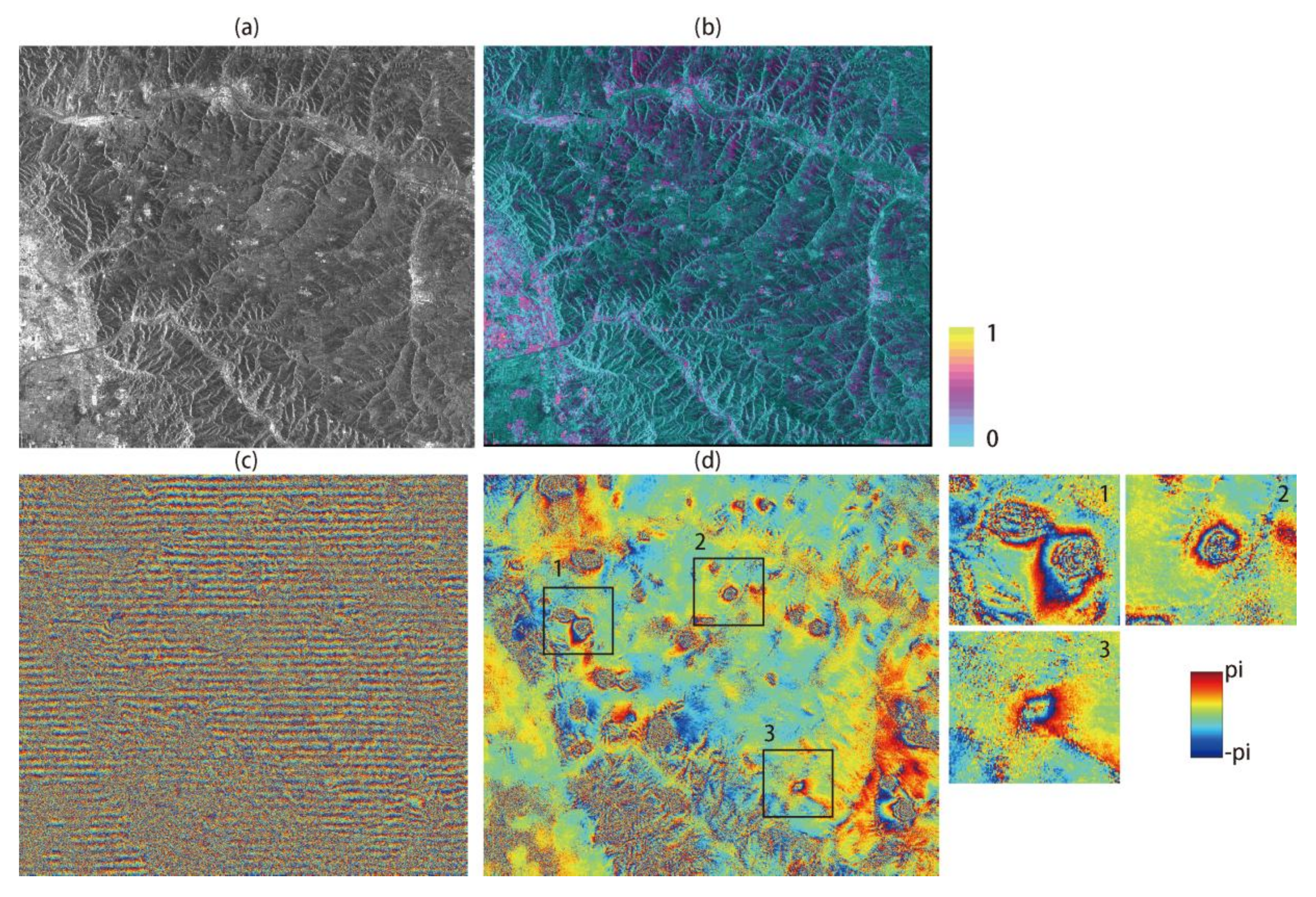
3.2.1. Datong Area
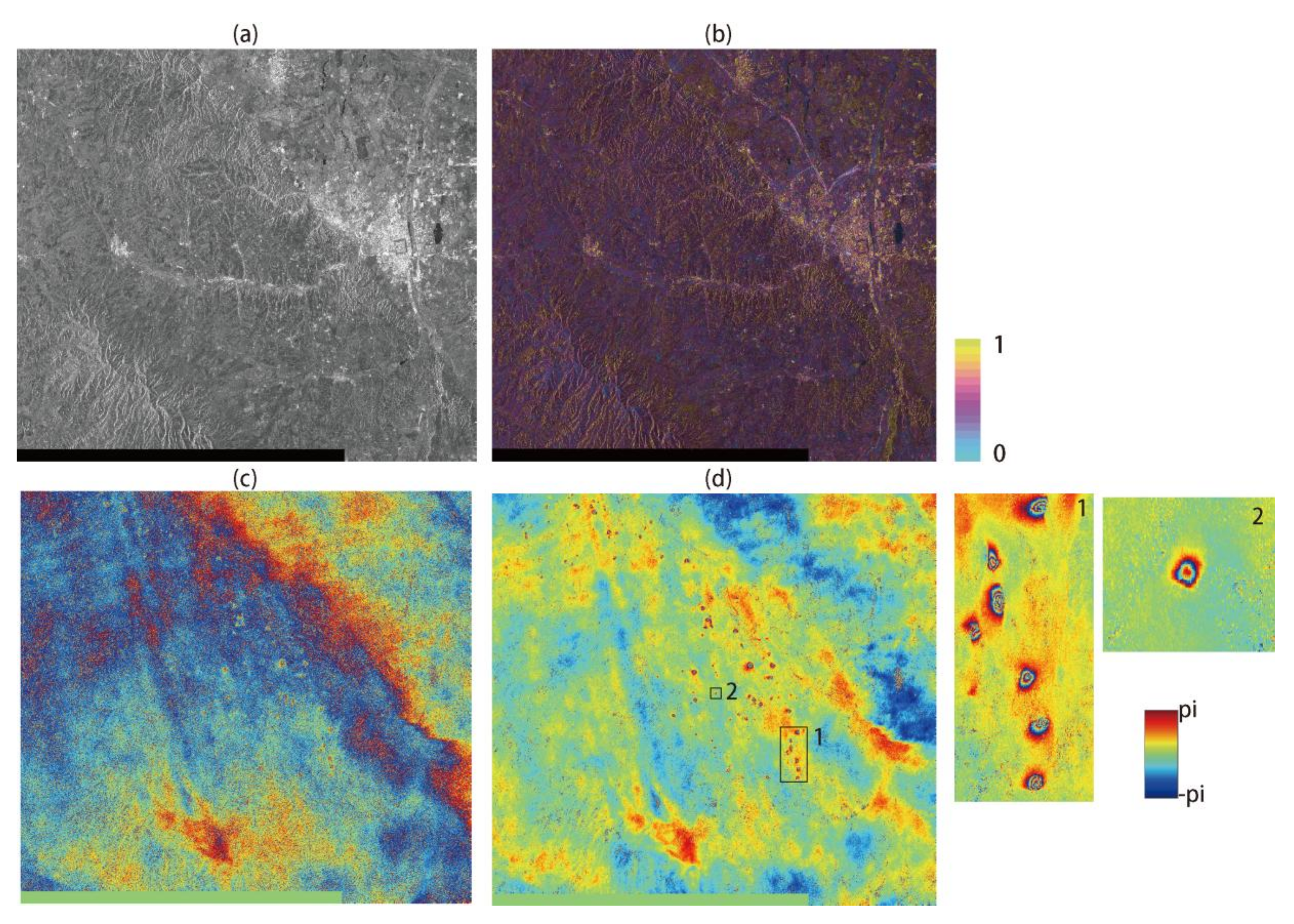
3.2.2. Tohoku-Oki Area
4. Discussion
5. Conclusions
Acknowledgments
Author Contributions
Conflicts of Interest
References
- Berardino, P.; Fornaro, G.; Lanari, R.; Sansosti, E. A new algorithm for surface deformation monitoring based on small baseline differential sar interferograms. IEEE Trans. Geosci. Remote Sens. 2002, 40, 2375–2383. [Google Scholar] [CrossRef]
- Ferretti, A.; Prati, C.; Rocca, F. Permanent scatterers in sar interferometry. IEEE Trans. Geosci. Remote Sens. 2001, 39, 8–20. [Google Scholar] [CrossRef]
- Massonnet, D.; Feigl, K.L. Radar interferometry and its application to changes in the earth’s surface. Rev. Geophys. 1998, 36, 441–500. [Google Scholar] [CrossRef]
- Diao, F.; Xiong, X.; Wang, R.; Zheng, Y.; Walter, T.R.; Weng, H.; Li, J. Overlapping post-seismic deformation processes: Afterslip and viscoelastic relaxation following the 2011 Mw9.0 Tohoku (Japan) earthquake. Geophys. J. Int. 2013, 196, 218–229. [Google Scholar] [CrossRef]
- Copley, A.; Hollingsworth, J.; Bergman, E. Constraints on fault and lithosphere rheology from the coseismic slip and postseismic afterslip of the 2006 Mw7.0 Mozambique earthquake. J. Geophys. Res. Solid Earth 2012, 117. [Google Scholar] [CrossRef]
- Liu, Y.; Xu, C.; Li, Z.; Wen, Y.; Chen, J.; Li, Z. Time-dependent afterslip of the 2009 Mw6.3 Dachaidan earthquake (China) and viscosity beneath the qaidam basin inferred from postseismic deformation observations. Remote Sens. 2016, 8, 649. [Google Scholar] [CrossRef]
- Fattahi, H.; Amelung, F. Insar uncertainty due to orbital errors. Geophys. J. Int. 2014, 199, 549–560. [Google Scholar] [CrossRef]
- Thiel, C.; Schmullius, C. Impact of tree species on magnitude of palsar interferometric coherence over siberian forest at frozen and unfrozen conditions. Remote Sens. 2014, 6, 1124–1136. [Google Scholar] [CrossRef]
- Zebker, H.A.; Villasenor, J. Decorrelation in interferometric radar echoes. IEEE Trans. Geosci. Remote Sens. 1992, 30, 950–959. [Google Scholar] [CrossRef]
- Ding, X.-L.; Li, Z.-W.; Zhu, J.-J.; Feng, G.-C.; Long, J.-P. Atmospheric effects on insar measurements and their mitigation. Sensors 2008, 8, 5426–5448. [Google Scholar] [CrossRef] [PubMed]
- Jiang, M.; Li, Z.; Ding, X.; Zhu, J.-J.; Feng, G. Modeling minimum and maximum detectable deformation gradients of interferometric sar measurements. Int. J. Appl. Earth Obs. Geoinf. 2011, 13, 766–777. [Google Scholar] [CrossRef]
- Xu, B.; Li, Z.-W.; Wang, Q.-J.; Jiang, M.; Zhu, J.-J.; Ding, X.-L. A refined strategy for removing composite errors of sar interferogram. IEEE Geosci. Remote Sens. Lett. 2014, 11, 143–147. [Google Scholar] [CrossRef]
- Rosen, P.A.; Hensley, S.; Peltzer, G.; Simons, M. Updated repeat orbit interferometry package released. Eos Trans. Am. Geophys. Union 2004, 85, 47. [Google Scholar] [CrossRef]
- Knedlik, S.; Loffeld, O.; Hein, A.; Arndt, C. A novel approach to accurate baseline estimation. In Proceedings of the IEEE 1999 International Geoscience and Remote Sensing Symposium (IGARSS’99), Hamburg, Germany, 28 June–2 July 1999; pp. 254–256. [Google Scholar]
- Pepe, A.; Berardino, P.; Bonano, M.; Euillades, L.D.; Lanari, R.; Sansosti, E. Sbas-based satellite orbit correction for the generation of dinsar time-series: Application to radarsat-1 data. IEEE Trans. Geosci. Remote Sens. 2011, 49, 5150–5165. [Google Scholar] [CrossRef]
- Kohlhase, A.; Feigl, K.; Massonnet, D. Applying differential inSAR to orbital dynamics: A new approach for estimating ERS trajectories. J. Geod. 2003, 77, 493–502. [Google Scholar] [CrossRef][Green Version]
- Biggs, J.; Wright, T.; Lu, Z.; Parsons, B. Multi-interferogram method for measuring interseismic deformation: Denali fault, Alaska. Geophys. J. Int. 2007, 170, 1165–1179. [Google Scholar] [CrossRef]
- Bähr, H.; Hanssen, R.F. Reliable estimation of orbit errors in spaceborne SAR interferometry. J. Geod. 2012, 86, 1147–1164. [Google Scholar] [CrossRef]
- Wang, H.; Wright, T.; Biggs, J. Interseismic slip rate of the northwestern Xianshuihe fault from inSAR data. Geophys. Res. Lett. 2009, 36. [Google Scholar] [CrossRef]
- Feng, G.; Ding, X.; Li, Z.; Jiang, M.; Zhang, L.; Omura, M. Calibration of an insar-derived coseimic deformation map associated with the 2011 Mw-9.0 Tohoku-oki earthquake. IEEE Geosci. Remote Sens. Lett. 2012, 9, 302–306. [Google Scholar] [CrossRef]
- Béjar-Pizarro, M.; Socquet, A.; Armijo, R.; Carrizo, D.; Genrich, J.; Simons, M. Andean structural control on interseismic coupling in the north Chile subduction zone. Nat. Geosci. 2013, 6, 462–467. [Google Scholar] [CrossRef]
- Gourmelen, N.; Amelung, F.; Lanari, R. Interferometric synthetic aperture radar–GPS integration: Interseismic strain accumulation across the Hunter Mountain fault in the eastern California shear zone. J. Geophys. Res. Solid Earth 2010, 115. [Google Scholar] [CrossRef]
- Shirzaei, M.; Walter, T.R. Estimating the effect of satellite orbital error using wavelet-based robust regression applied to inSAR deformation data. IEEE Trans. Geosci. Remote Sens. 2011, 49, 4600–4605. [Google Scholar] [CrossRef]
- Bähr, H. Orbital Effects in Spaceborne Synthetic Aperture Radar Interferometry; KIT Scientific Publishing: Karlsruhe, Germany, 2013. [Google Scholar]
- Zebker, H.A.; Chen, K. Accurate estimation of correlation in inSAR observations. IEEE Geosci. Remote Sens. Lett. 2005, 2, 124–127. [Google Scholar] [CrossRef]
- Spagnolini, U. 2-D phase unwrapping and instantaneous frequency estimation. IEEE Trans. Geosci. Remote Sens. 1995, 33, 579–589. [Google Scholar] [CrossRef]
- Jiang, M.; Ding, X.; Li, Z. Hybrid approach for unbiased coherence estimation for multitemporal inSAR. IEEE Trans. Geosci. Remote Sens. 2014, 52, 2459–2473. [Google Scholar] [CrossRef]
- Holland, P.W.; Welsch, R.E. Robust regression using iteratively reweighted least-squares. Commun. Stat. Theory Methods 1977, 6, 813–827. [Google Scholar] [CrossRef]
- Bishop, C.M. Pattern Recognition and Machine Learning; Springer: Berlin, Germany, 2006. [Google Scholar]
- Okada, Y. Surface deformation due to shear and tensile faults in a half-space. Bull. Seismol. Soc. Am. 1985, 75, 1135–1154. [Google Scholar]
- Jiang, M.; Ding, X.; Li, Z.; Tian, X.; Zhu, W.; Wang, C.; Xu, B. The improvement for baran phase filter derived from unbiased inSAR coherence. IEEE J. Sel. Top. Appl. Earth Obs. Remote Sens. 2014, 7, 3002–3010. [Google Scholar] [CrossRef]
- Hanssen, R.F. Radar Interferometry: Data Interpretation and Error Analysis; Springer: New York, NY, USA, 2001; Volume 2. [Google Scholar]
- Jiang, M.; Yong, B.; Tian, X.; Malhotra, R.; Hu, R.; Li, Z.; Yu, Z.; Zhang, X. The potential of more accurate insar covariance matrix estimation for land cover mapping. ISPRS J. Photogramm. Remote Sens. 2017, 126, 120–128. [Google Scholar] [CrossRef]
- Chen, C.W.; Zebker, H.A. Phase unwrapping for large SAR interferograms: Statistical segmentation and generalized network models. IEEE Trans. Geosci. Remote Sens. 2002, 40, 1709–1719. [Google Scholar] [CrossRef]
- Jónsson, S.; Zebker, H.; Segall, P.; Amelung, F. Fault slip distribution of the 1999 Mw7.1 Hector mine, California, earthquake, estimated from satellite radar and GPS measurements. Bull. Seismol. Soc. Am. 2002, 92, 1377–1389. [Google Scholar] [CrossRef]
- Feigl, K.L.; Thurber, C.H. A method for modelling radar interferograms without phase unwrapping: Application to the M 5 Fawnskin, California earthquake of 1992 December 4. Geophys. J. Int. 2009, 176, 491–504. [Google Scholar] [CrossRef]


| Location | Sensor | Track | Master (yyyy-mm-dd) | Slave (yyyy-mm-dd) | (m) | Pass | Char. Def. |
|---|---|---|---|---|---|---|---|
| Datong | GF-3 | - | 2017-04-01 | 2017-06-27 | 536 | D | local |
| Datong | Sentinel-1 | 40 | 2015-10-15 | 2015-10-27 | 87 | A | local |
| Tohoku-Oki | ASAR | 347 | 2011-02-19 | 2011-03-21 | 163 | D | global |
| Tohoku-Oki | ASAR | 74 | 2011-03-02 | 2011-04-01 | −121 | D | global |
| Sensor | Track | Unit Vector of LOS [East North Up] | Number of GPS Station | RMSE before Correction (cm) | RMSE after Correction (cm) | RMSE Reduction (%) |
|---|---|---|---|---|---|---|
| ASAR | 347 | [0.64 0.11 0.75] | 97 | 35.55 | 9.52 | 73.22 |
| ASAR | 74 | [0.65 0.11 0.75] | 23 | 12.24 | 8.39 | 31.45 |
© 2018 by the authors. Licensee MDPI, Basel, Switzerland. This article is an open access article distributed under the terms and conditions of the Creative Commons Attribution (CC BY) license (http://creativecommons.org/licenses/by/4.0/).
Share and Cite
Tian, X.; Malhotra, R.; Xu, B.; Qi, H.; Ma, Y. Modeling Orbital Error in InSAR Interferogram Using Frequency and Spatial Domain Based Methods. Remote Sens. 2018, 10, 508. https://doi.org/10.3390/rs10040508
Tian X, Malhotra R, Xu B, Qi H, Ma Y. Modeling Orbital Error in InSAR Interferogram Using Frequency and Spatial Domain Based Methods. Remote Sensing. 2018; 10(4):508. https://doi.org/10.3390/rs10040508
Chicago/Turabian StyleTian, Xin, Rakesh Malhotra, Bing Xu, Haoping Qi, and Yuxiao Ma. 2018. "Modeling Orbital Error in InSAR Interferogram Using Frequency and Spatial Domain Based Methods" Remote Sensing 10, no. 4: 508. https://doi.org/10.3390/rs10040508
APA StyleTian, X., Malhotra, R., Xu, B., Qi, H., & Ma, Y. (2018). Modeling Orbital Error in InSAR Interferogram Using Frequency and Spatial Domain Based Methods. Remote Sensing, 10(4), 508. https://doi.org/10.3390/rs10040508