A Multilayer Surface Temperature, Surface Albedo, and Water Vapor Product of Greenland from MODIS

Abstract

A multilayer, daily ice surface temperature (IST)–albedo–water vapor product of Greenland, extending from March 2000 through December 2016, has been developed using standard MODerate-resolution Imaging Spectroradiometer (MODIS) data products from the Terra satellite. To meet the needs of the ice sheet modeling community, this new Earth Science Data Record (ESDR) is provided in a polar stereographic projection in NetCDF format, and includes the existing standard MODIS Collection 6.1 IST and derived melt maps, and Collection 6 snow albedo and water vapor maps, along with ancillary data, and is provided at a spatial resolution of ~0.78 km. This ESDR enables relationships between IST, surface melt, albedo, and water vapor to be evaluated easily. We show examples of the components of the ESDR and describe some uses of the ESDR such as for comparison with skin temperature, albedo, and water vapor output from Modern Era Retrospective analysis for Research and Applications, Version 2 (MERRA-2). Additionally, we show validation of the MODIS IST using in situ and aircraft data, and validation of MERRA-2 skin temperature maps using MODIS IST and in situ data. The ESDR has been assigned a DOI and will be available through the National Snow and Ice Data Center by the summer of 2018.

1. Introduction

The rate of mass loss of the Greenland Ice Sheet has increased in recent decades. Increases in both ice discharge and surface meltwater runoff have been documented but the relative contribution of surface runoff is greater [1] and models predict a larger contribution to sea level rise from surface melt and runoff in the future [1,2]. A combination of in situ and satellite measurements, and modeling, is needed to assess ice sheet surface–mass balance (SMB) and, thus, the contribution of ice sheet meltwater to sea level rise. While satellites can obtain accurate measurements of the ice sheet surface under clear-sky conditions, clouds preclude measurement of the entire ice sheet surface at the same time. In addition, ice sheet SMB cannot be determined based on in situ measurements alone, in part due to the low density of meteorological stations on the ice sheet surface.

Skin temperature of the Greenland Ice Sheet must be known for estimation and modeling of SMB and ice sheet processes. The skin temperature is the temperature at the interface between the surface and the atmosphere. It is often also referred to as the ice surface temperature (IST). Skin temperature affects basal melt and internal temperature of the ice sheet, largely controls runoff, and is a fundamental input for dynamical ice sheet models [3,4] because it is an important component of the ice sheet radiation budget and mass balance. Model output should be validated using in situ and satellite-derived measurements, when possible.

Following the launch of the MODerate-resolution Imaging Spectroradiometer (MODIS) on the Terra satellite in 1999, swath-based and daily gridded images and data products of the ice sheet became available in early 2000. A second MODIS was launched on the Aqua satellite in 2002. An Earth Science Data Record (ESDR) of IST, extending from 2000 to 2012, was produced using primarily Terra MODIS data [5,6]. For the present work, we developed an enhanced ESDR using data from IST, daily albedo, and atmospheric water vapor (WV) standard Terra MODIS products. The new ESDR provides the data products on the same grid, thus facilitating studies of the complex relationships between IST, melt, albedo, and WV. The earlier ESDR of IST from MODIS has been extended in time and upgraded with improved spatial resolution (~0.78 km), use of the most up-to-date MODIS data processing from Collection 6 (C6) and Collection 6.1 (C6.1), and additional fields of information.

2. Description of the Dataset in the New Earth Science Data Record

Standard MODIS swath products are provided from C6.1 MOD29 IST and C6 MOD05 water vapor data products. Daily products are provided from the C6 MOD10 albedo standard product. These standard products have been gridded to a polar stereographic grid https://nsidc.org/data/polar-stereo/ps_grids.html. The daily and monthly IST and water vapor products in the ESDR were derived from the standard swath products, while daily albedo product is used since there is no albedo swath product, and the monthly albedo product was derived from the standard daily albedo product. A detailed ice sheet mask [7], an outline of the eight major drainage basins of the ice sheet [8], and metadata are also provided as ancillary data. Cloud obscuration is determined from the cloud mask, MOD35 [9] [https://modis-atmos.gsfc.nasa.gov/sites/default/files/ModAtmo/CMUSERSGUIDE_0.pdf], an input product to the MOD10 and MOD29 algorithms. All product files, as described below, are NetCDF in a polar stereographic projection in the following data layers.

• Swath Maps. Terra MODIS swaths of IST, surface melt, atmospheric WV, WV quality assurance (QA), and cloud mask QA (from the WV product) are provided. All available swaths covering Greenland for each day (24 h period) are provided and used to produce the daily IST and WV maps. For the MOD10 daily albedo, in this data layer, a daily product is provided instead of swath data because it is not available as a swath product.
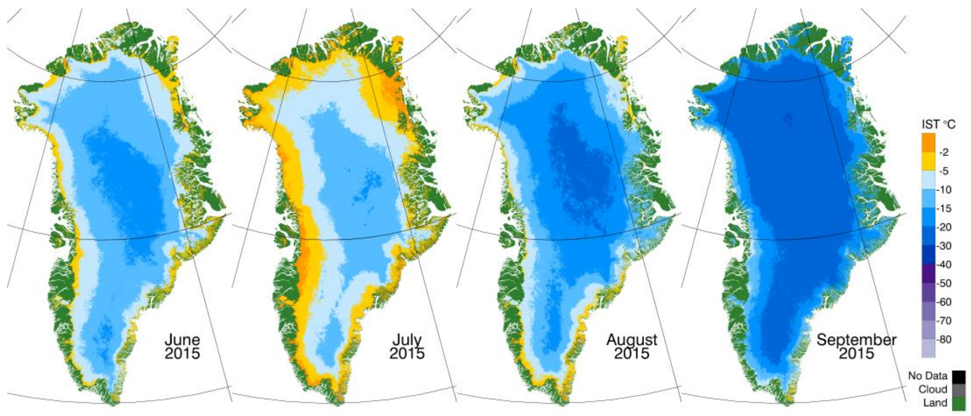
• Daily Maps. Four maps are provided for each day: IST, surface melt, albedo, and WV. Also provided is the “IST swath tracker” that allows a user to easily locate the IST swath that was used to create each daily IST map.
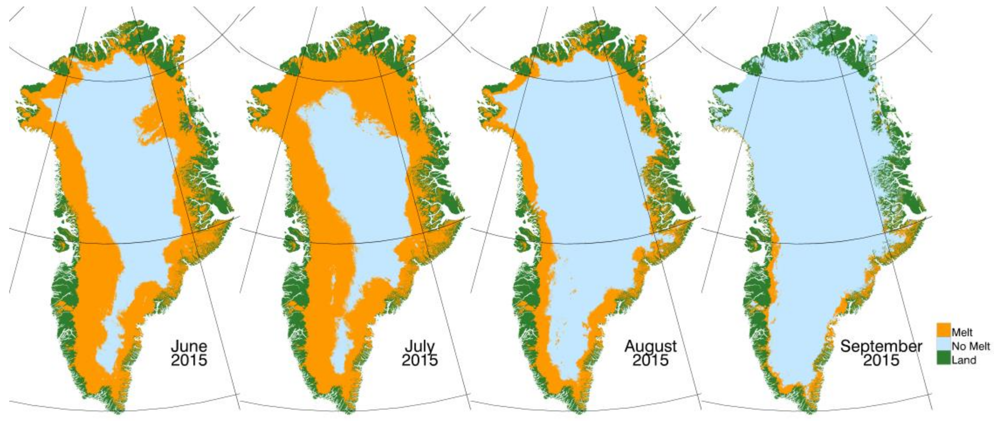
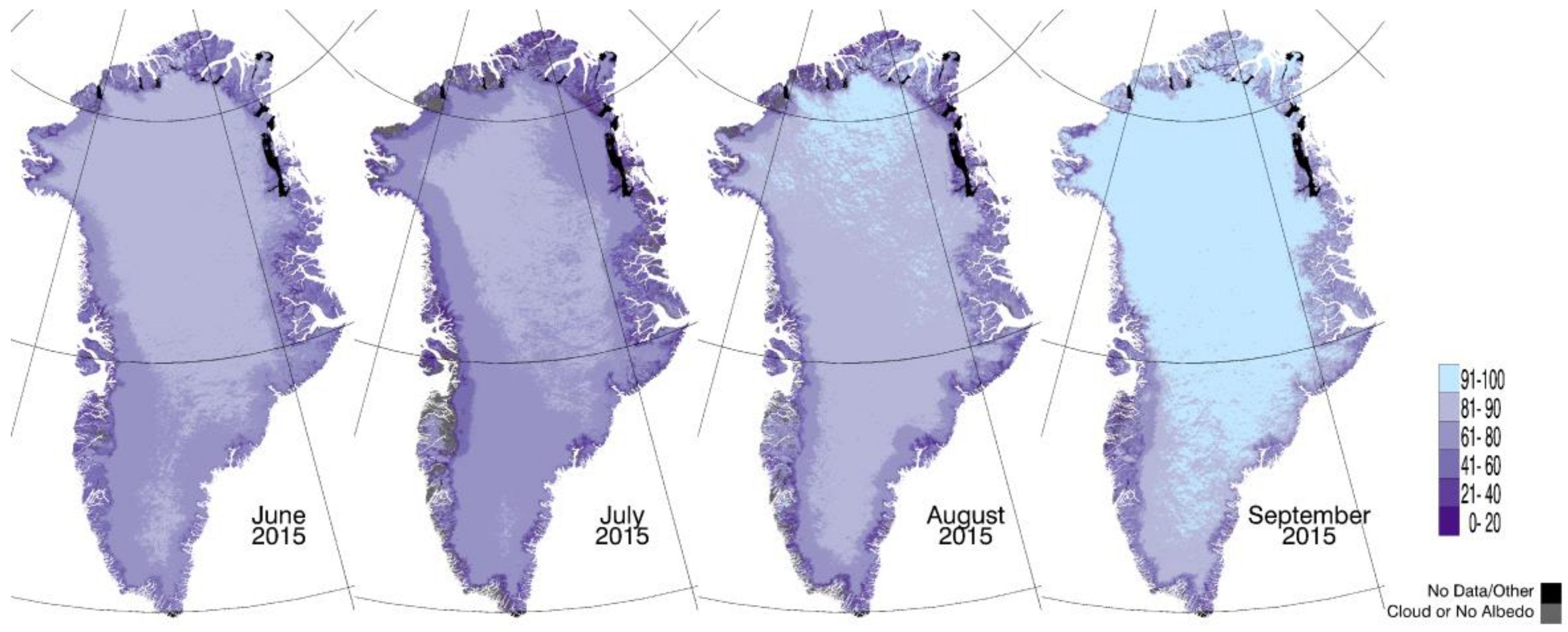
• Monthly Maps. For each grid cell of each monthly map, all clear-sky cells (as determined from the MODIS cloud mask) are averaged from each daily map to produce a monthly map consisting of up to 28–31 days of data, depending on the length of the month. Seven maps are provided for each month: IST mean, IST number-of-days, number of melt days, albedo, albedo number-of-days, WV mean, and WV number-of-days. The ‘number-of-days’ maps provide the number of days that contributed to developing the monthly averages for each grid cell.
  For the WV map, the number of days is not dependent on a cloud mask since there is no cloud masking; however, darkness and missing data preclude obtaining a WV value and, therefore, the number-of-days reported may be less than the number of days in a month.
• Ancillary Data. Included in this layer are five separate fields consisting of (1) latitude, (2) longitude, (3) land/water/ice mask, (4) drainage basin mask, and (5) grid cell size (pixel area). Grid cell size information is provided to facilitate calculation of areal extent since the polar stereographic map is not an equal area projection.

For the daily IST data, the information containing the number of swaths that contributed to the daily IST for each cell can be extracted from the “swath tracker” layer.

The standard MODIS IST and water vapor products are swath-based and, thus, ungridded. The native grid of the daily albedo product is sinusoidal. The products in the ESDR are gridded into a polar stereographic grid to a common spatial resolution at 0.78125 km resolution.

Ice Surface Temperature (IST). The daily maps are produced by averaging the ISTs in the pixels for all of the Terra swaths available for each 24 h period, and then gridding that data into cells of a polar stereographic projection. Grid cells that are cloudy, according to the cloud mask, do not provide IST and are therefore not used to calculate the value reported in that grid cell in the daily map. The daily maps are averaged (for each grid cell) to create monthly maps (Figure 1) for each month of the MODIS Terra time series. From the swath, daily, or monthly maps, mean annual clear-sky IST maps can be created by a user.

Surface Melt. The daily surface melt product is calculated using IST data from non-cloud-obscured pixels. If an IST is ≥−1 °C then it is considered “melt.” The melt threshold of ≥−1 °C is used instead of ≥0 °C for three reasons: (1) The accuracy of the IST product is ±1 °C and, therefore, melt would be missed if a threshold of ≥0 °C was used. (2) This melt threshold yields a map that is closer to other remotely sensed maps. (3) Melt can occur while temperatures are slightly below freezing if the solar radiation is strong. However, a user may select any threshold value desired to create a melt map from the IST data. Daily and monthly (Figure 2) maximum melt products are provided. From the swath, daily, or monthly maps, a user can create annual maps of maximum surface melt, as shown in Figure 3; these were developed by using the monthly melt maps to calculate the maximum annual melt.

Albedo. The C6 MOD10A1 snow product provides the daily snow albedo [10] that is used in the present product. A C6.1 MOD10A1 product will be produced in the near future, but it is not yet available. The MOD10A1 daily snow albedo algorithm, both developed and first validated by Klein and Stroeve [11], has also been evaluated over Greenland by Stroeve et al. [12] and has been used by many investigators (e.g., [13,14,15,16,17]. The MOD10A1 albedo algorithm is based on a model of bidirectional reflectance of snow to correct for anisotropic scattering effects over non-forested surfaces [11]. In the new ESDR, daily and monthly (Figure 4) albedo maps are provided.

Water Vapor (WV). The algorithm used to develop the daily MODIS water vapor product (MOD05) relies on observations of attenuation of near-IR solar radiation reflected by surfaces and clouds using ratios of water vapor absorbing channels [18]. The column WV is derived from transmittances that are based on theoretical calculations and look-up tables. Typical errors in the derived values range from 5 to 10 percent [18]. Swath, daily, and monthly (Figure 5) WV maps of Greenland are provided in the ESDR. This product is available during all sky conditions except for darkness. For clear pixels, the WV retrievals are made above clear surfaces. For cloudy pixels, the WV retrievals are made above clouds. The water vapor below clouds is not seen by MODIS near-IR channels; this could result in biases when using a time series of WV data.

Collection 6.1 MOD05 WV was not available when the new ESDR was produced so C6 MOD05 was used, though C6.1 has recently become available. Comparisons between the C6 and C6.1 WV maps reveal very small differences over Greenland. For example, for three different MOD05 swaths acquired in 2014—on 10 April, 29 June, and 17 September, respectively—we found that over 99.5% of the C6 and C6.1 pixels in common on each C6 and C6.1 swath studied (2,748,505 pixels each) agreed within ±0.1 cm of water.

Ice Mask and Delineation of Drainage Basins. A land/water/ice mask from the Greenland Ice Mapping Project [7] is provided in the ancillary data layer. There is also a separate field delineating eight major drainage basins as well as the sub-basins, developed from ICESat vector data [8], as shown in Figure 6. Basin 1 has four sub-basins; Basins 3 and 4 have three; Basins 2, 6, 7, and 8 have two; and Basin 5 has no sub-basins.

3. Differences between the Current Multilayer ESDR and the Earlier ESDR of IST

Compared with the earlier MODIS IST ESDR of Greenland [5], the new ESDR has the following differences.

• There are three MODIS products (IST, albedo, and water vapor) and one derived product (surface melt) in the new ESDR, versus two (IST and surface melt) in the earlier one.
• Collection 6 and 6.1 MODIS Terra data are used in the new ESDR as compared to Collection 5 in the earlier one.
• The calibration of the MODIS Terra data has been improved by the MODIS Characterization Support Team (MCST) to take into account sensor degradation that is particularly notable in the visible bands [19]. Polashenski et al. [20] showed that previously published trends of dramatically declining albedo over Greenland were due to uncorrected sensor degradation in C5 products, rather than to actual geophysical trends of albedo decline. Following on from that work, Casey et al. [21] showed that the C6 MOD10A1 albedo products now have a very weak trend of declining albedo from 2001 to 2016, after corrections for sensor degradation in input bands were instituted by MCST for C6 [19].
• The spatial resolution of the new ESDR is 0.78125 km versus 1.5625 km for the earlier IST–melt product. Because the inherent resolution of the MOD29 IST product is 1 km, subsampling was needed to achieve ~0.78 km resolution using MODIS reprojection tools [https://lpdaac.usgs.gov/tools/modis_reprojection_tool] and nearest-neighbor binning methods. To take advantage in the future of the improved resolution (750 m) of the Visible Infrared Imaging Radiometer Suite (VIIRS) product for data product continuity, we decided on ~0.78 km as the resolution of the new ESDR. This allows for a multisensor ESDR that will include both MODIS and VIIRS IST. We use 0.78125 km, which is compatible with an even multiple of the standard 25, 12.5, 6.25 km Special Sensor Microwave Imager Polar Stereographic grid.
• The land/water/ice mask [7] used in the new product is much more detailed than the land/water/ice mask that was used in the earlier product.
• The daily maps of the new product are developed using all available swaths in a 24 h period, versus using all available swaths in a 6 h period focused on the warmest part of the day to emphasize maximum daily melt. A sample day, 3 July 2012, of the IST is shown in Figure 7 (Right image). On this day there were 23 MODIS Terra swaths available to develop the daily product.

C6 and C6.1 Specific Issues Regarding the Ice Surface Temperature Product, MOD29. Sensor degradation has not been an issue for MODIS bands 31 and 32 which are used to develop IST maps of sea ice and Greenland in both C5 and C6.1. However, small adjustments were made by MCST [19], with expected differences in C6.1 minus C5 temperatures of up to −0.2 K, meaning that the C6.1 temperatures are slightly lower than the C5 temperatures. Our preliminary measurements have shown that this difference in IST varies from −0.06 to −0.26 K over Greenland (

Table 1. Comparison of clear-sky ‘pixels in common’ in Collection 5 and Collection 6.1 derived from MODIS Terra MOD29 swaths for winter, spring, summer, and fall 2012. The difference in IST is calculated as follows: C6.1 IST minus C5 IST; the negative values mean that the C6.1 ISTs are lower.

Date and Time (UTC) of Swaths	Number of Pixels in Common	Difference in IST (K)
01 Jan 16:15	818,184	−0.26
03 April 15:45	1,095,759	−0.06
09 July 15:45	967,589	−0.20
13 Oct 14:50	756,328	−0.14

).

Though the ISTs under clear skies are very similar between C5 and C6.1 [19], as described above and shown in Table 1, when we look at a time series of IST data of Greenland from the earlier ESDR [22] compared with a time series from the new ESDR, we see important differences. For the earlier ESDR the averaging of IST swaths focused on the warmest part of each day, to create the daily maps whereas the new ESDR averages swath data acquired over a 24 h period each day. Additionally, there were changes in cloud masking over Greenland from C5 to C6 and C6.1, that could potentially affect time-series results and trend calculations.

The University of Wisconsin [9] concluded that in the C5 Level 1b Terra data, several IR bands were noticeably warmer (~3 K) than the Aqua bands (compared with Atmospheric Infrared Sounder data) in scenes with very cold temperatures, such as those that cover Greenland. One of these was MODIS band 29, used along with band 31 in the snow detection algorithm internal to the cloud masking algorithm, leading to “no snow” decisions in many cases even though normalized difference snow index values indicated snow. A change was made for C6 [19,23,24] and C6.1 [25,9]. Our preliminary studies indicate that the C6.1 cloud mask, as is the case with the C5 cloud mask, may still be missing some clouds. Areas that have the shape of clouds but are not masked by the C6.1 MOD35 cloud mask are visible on many of the C6.1 IST daily maps, including the one shown in Figure 7. Additional work is needed to assess the accuracy of the C6.1 cloud mask over Greenland.

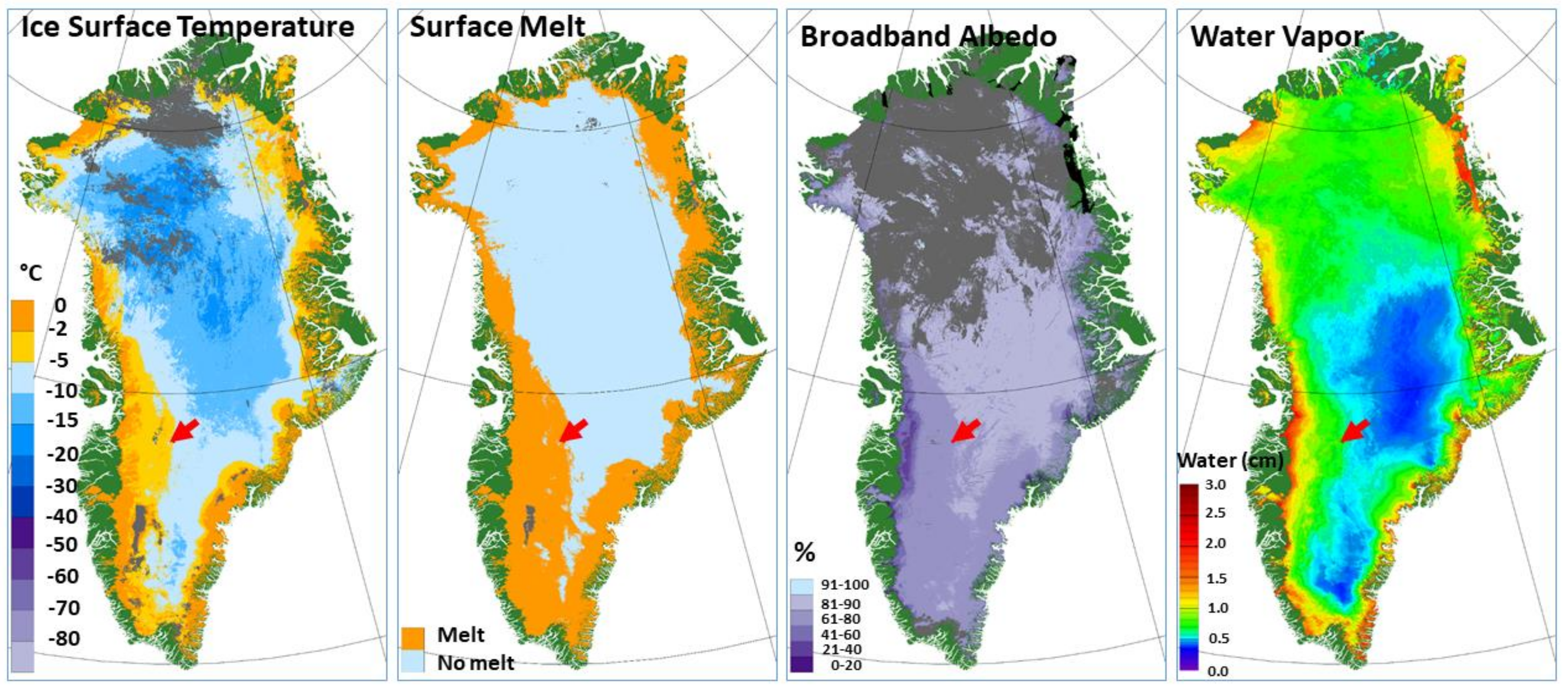
4. Relationships between Map Products

Multiple maps on the same grid enable geophysical parameters to be compared and relationships to be investigated. For example, the relationship between surface melt and albedo can be explored easily, as illustrated in Figure 8, and discussed in Mortimer and Sharp [26]. Surface melt is associated with lower albedo because the snow grain size increases with melting. After the surface refreezes, the albedo will increase again, but will not get as high as it was when the snow was fresh. Note also the higher water vapor values on the periphery of the ice sheet, and especially in the area of the boundary seen in the albedo map. Of course, the color selections can be adjusted to emphasize or to de-emphasize relationships on any color-coded map, but Figure 8 is illustrative of the kinds of relationships a user might want to explore.

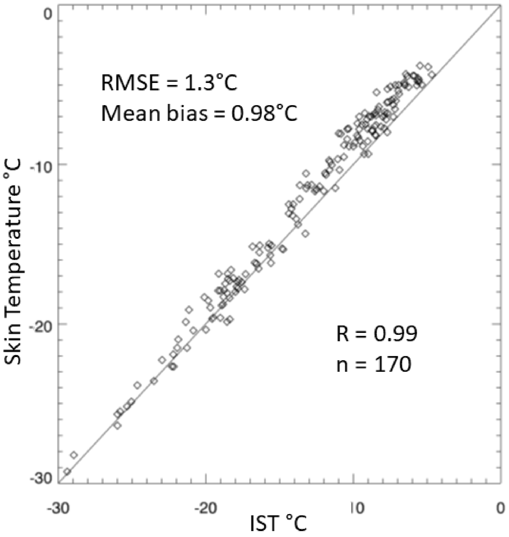
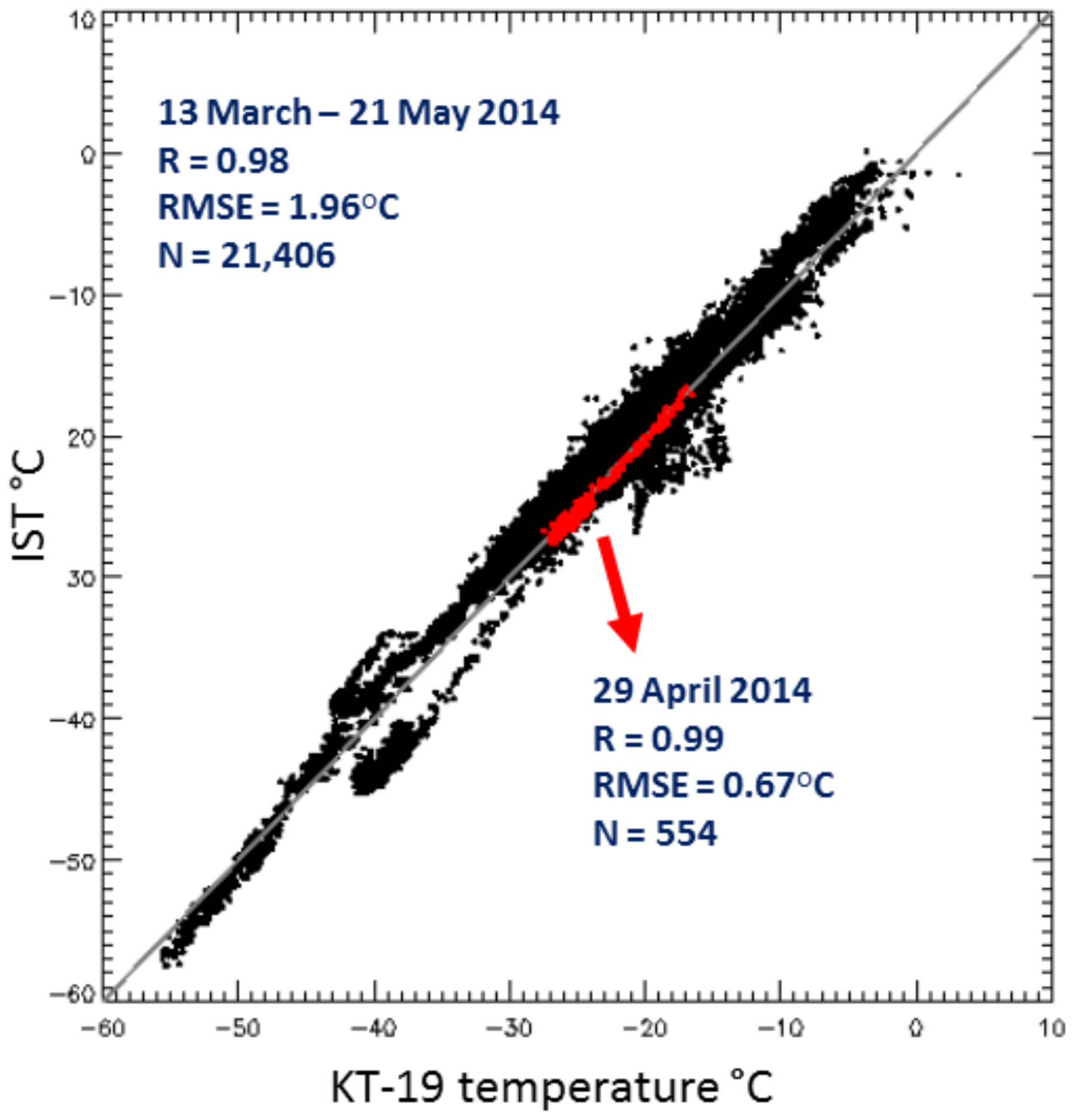
5. Validation of IST

There is currently no way to validate MOD29 IST, MOD10 albedo, and MOD05 water vapor in an absolute sense for the entire ice sheet, though comparisons can be made with other products, such as from maps derived from reanalysis models. In situ data have been used to validate discrete portions of the C6.1 MOD29 IST swath data as described in the next section.

There are NOAA weather stations on the ice sheet that measure air temperature, but most of them are automatic weather stations (AWS) that may not be maintained frequently and, thus, the data may have large uncertainties [27,28]. The temperature sensors at Summit Station near Summit Camp are maintained daily and provide high-quality air temperature measurements at a nominal height of 2 m, but these values are not directly comparable to the IST (skin temperature) measurements (see [5,27,29]). It has long been known that the 2 m air temperature and the IST, though highly correlated, are often quite different, and that the relationship between 2 m air temperature and IST varies under different atmospheric conditions; more discussion on this topic is provided in Adolph et al. [29].

A winter cold bias has been identified in time series of satellite data of IST because satellite measurements of the surface cannot be made through cloud cover, and cloud cover tends to warm the ice sheet surface due to positive feedback effects (e.g., [5]). The result is that the satellite sensor is not measuring the IST when the surface tends to be warmer (i.e., under cloud cover).

Another cold bias has been discussed in prior work that has been attributed to MODIS sensor calibration issues at very low temperatures (e.g., about −20 °C and lower) [5,27]. However, recent work calls this into question. When skin temperature (versus 2 m air temperature) is compared with MODIS-derived ISTs, the cold bias at very low temperatures is not evident [29], indicating that the suspected cold bias seen in earlier work may in fact be due to problems inherent in validation studies conducted using 2 m air temperatures. Adolph et al. [29] suggest that the difference between the 2 m air temperature and the skin temperature may be greater at very low temperatures (e.g., ~−20 °C and lower) as compared to temperatures closer to 0 °C; therefore, there may not be a cold bias in the MODIS data. More work is needed to investigate this issue.

Comparison with field measurements. For a 40 day study period from 8 June to 18 July 2015, measurements of the ice sheet skin temperature were obtained at a location about 10 km north-northwest of Summit (72.65923°N, −38.57067°W) by Adolph et al. [29]. As part of this work, additional cloud screening was conducted over and above that which is done automatically by virtue of using the IST product with its internal MOD35 cloud mask. A Millimeter wavelength Cloud Radar (MMCR) operating at Summit Station identified clouds that were not detected by MOD35, resulting in more scenes being excluded from the dataset. Further visual cloud screening was also conducted using C6.1 MOD29 swath data for each day of the 40 day study period. All of the swaths during the study period were inspected visually, and an additional 26 swaths for which clouds appeared to contaminate the pixel in which the field measurements were acquired, were removed. With the 170 remaining IST–skin temperature pairs (Figure 9), RMSE = 1.30 °C, and in situ derived skin temperature and MOD29 ISTs is highly correlated (R = 0.99) (N = 170). There is a mean bias of 0.98 °C with the MOD29 being colder than in situ measurements. This cold bias has been observed in both the MODIS land surface temperature (LST) and IST data, and is in agreement with previous work [30]. In all cases of visual screening when the temperature difference (skin versus IST) was >~1 deg, MOD29 was colder than the measured skin temperature.

Validation using KT-19 data from IceBridge. NASA IceBridge data acquired over Greenland on multiple flights flown from 13 March through 21 May 2014 were compared with the IST data from the new ESDR. After some visual cloud screening, we compared 21,406 temperatures derived from the IceBridge KT-19 infrared radiometer with ISTs from the ESDR (Figure 10); this yielded a correlation of R = 0.98, RMSE = 1.96 °C, N = 21,406, though visual inspection revealed that a large amount of cloud contamination remained. A relatively cloud-free swath acquired at 16:55 UTC on 29 April 2014 that contained 554 points (see red points in the scatter plot in Figure 10) reveals a better correlation between the IST in the ESDR and KT-19 temperatures, with R = 0.99 and RMSE = 0.67 °C, N = 554. The KT-19 temperatures within each IST cell were averaged to produce one value. The difference in temperature between the C6.1 MOD29 ISTs and the KT-19 skin temperatures is generally <1 °C.

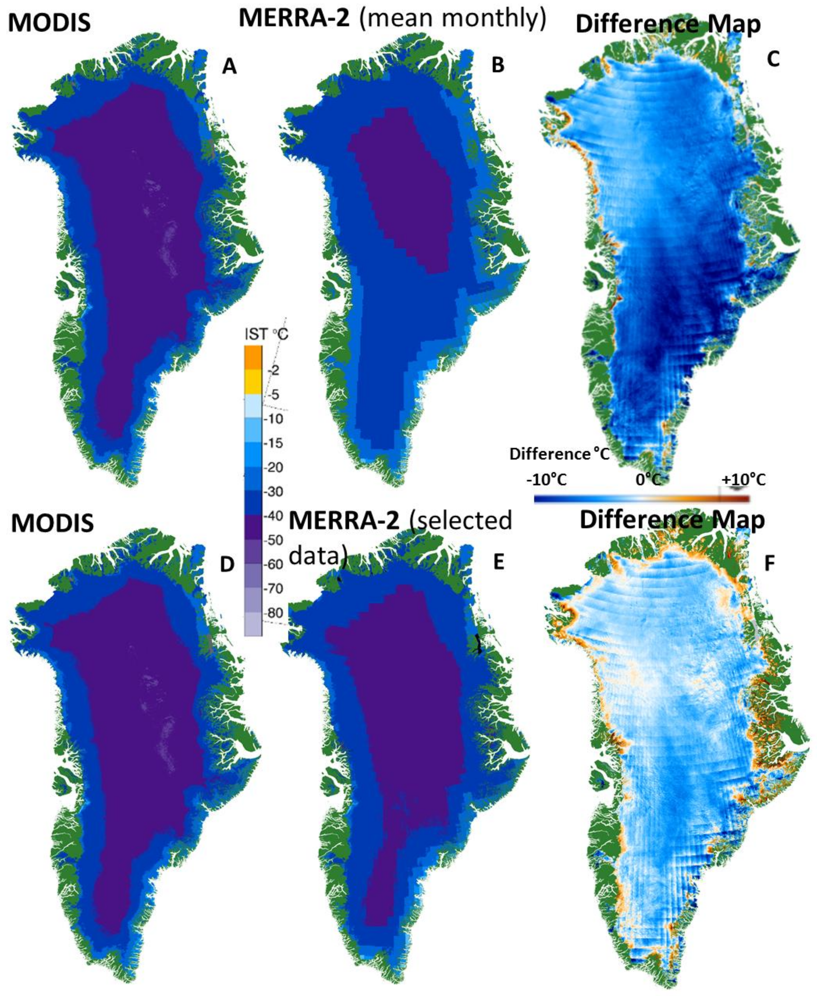
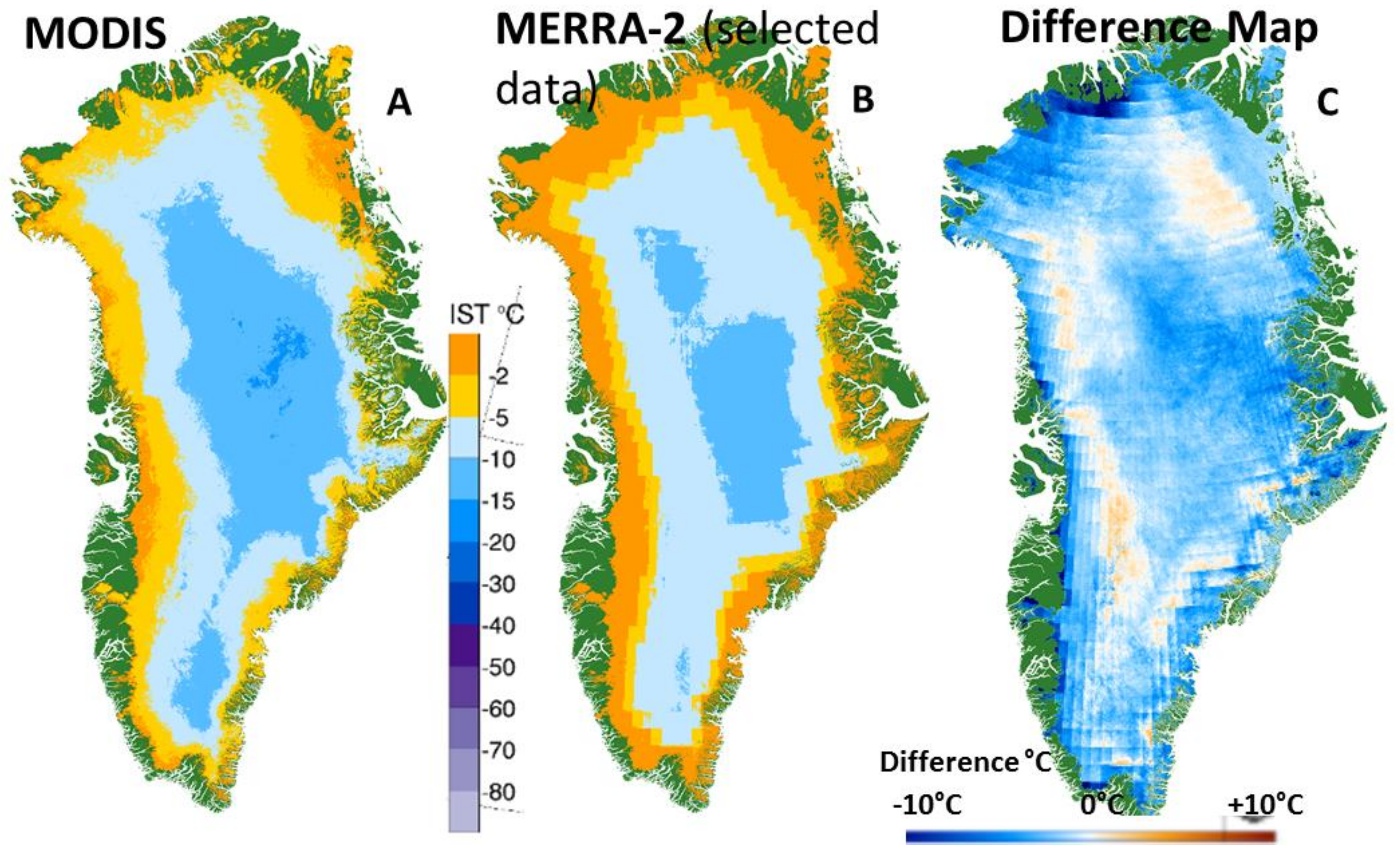
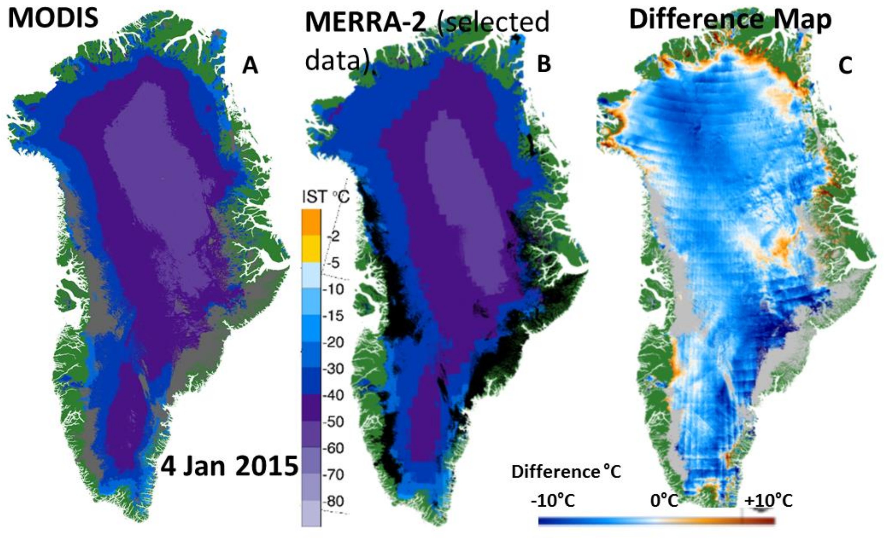
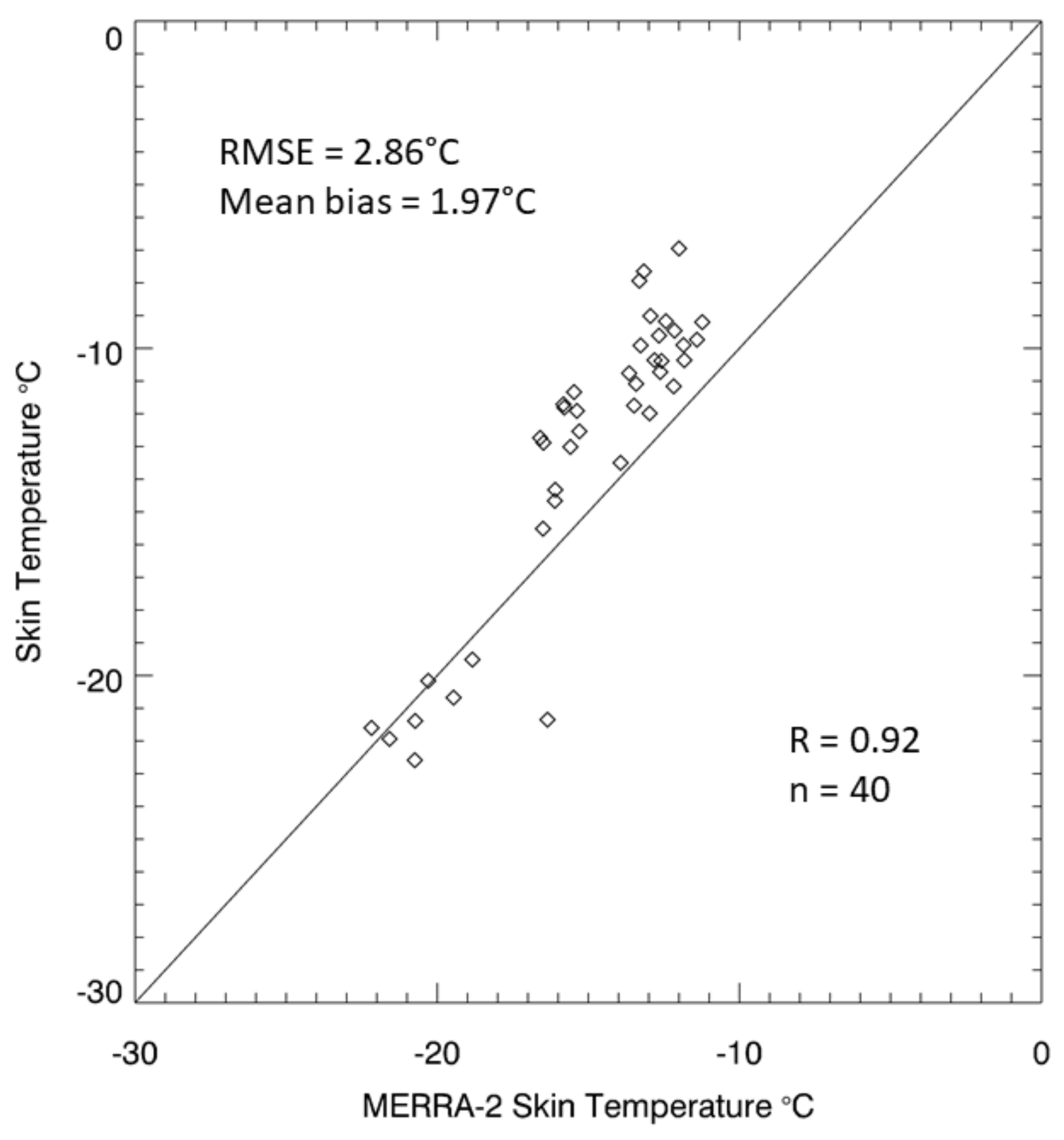
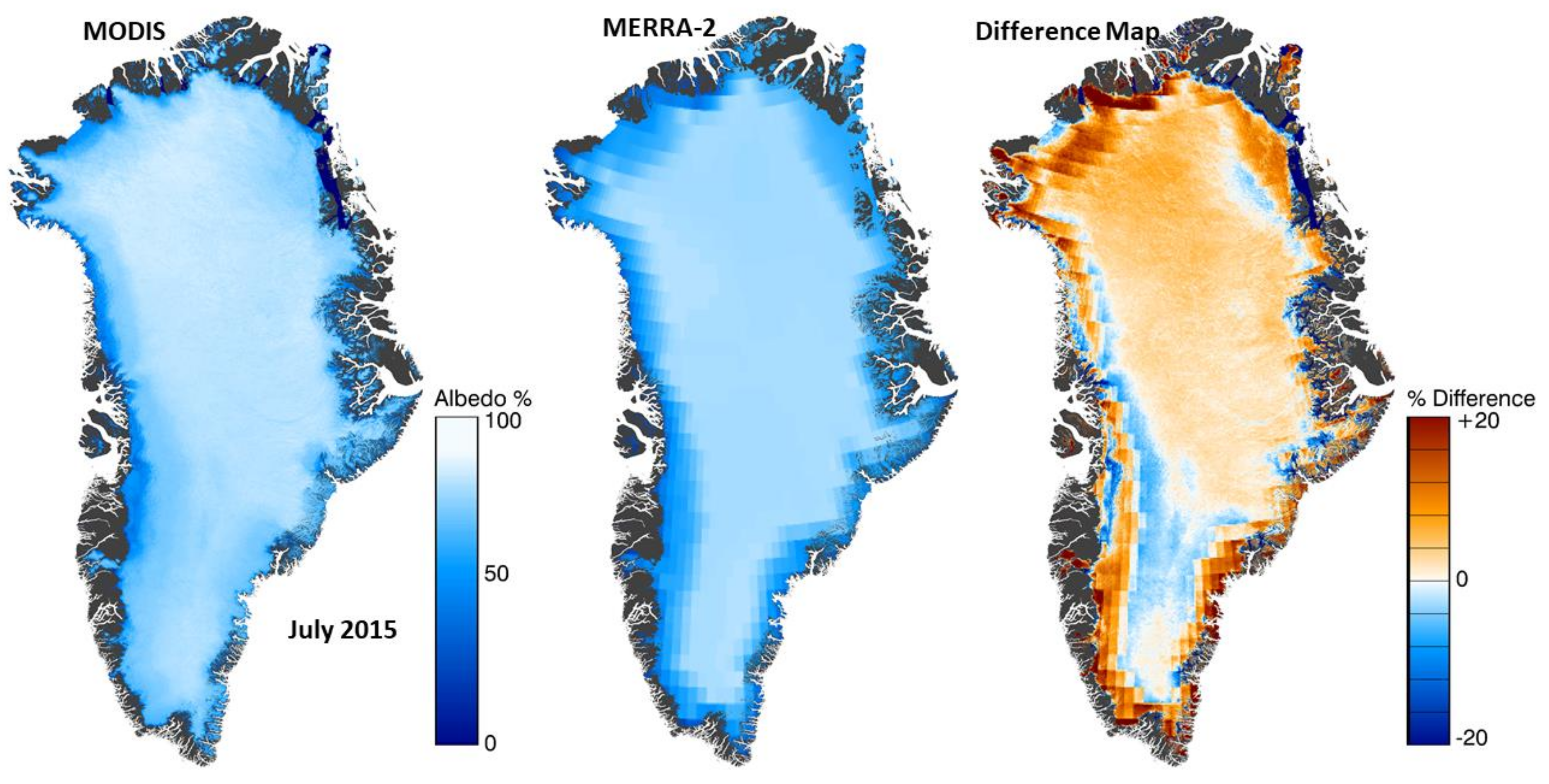
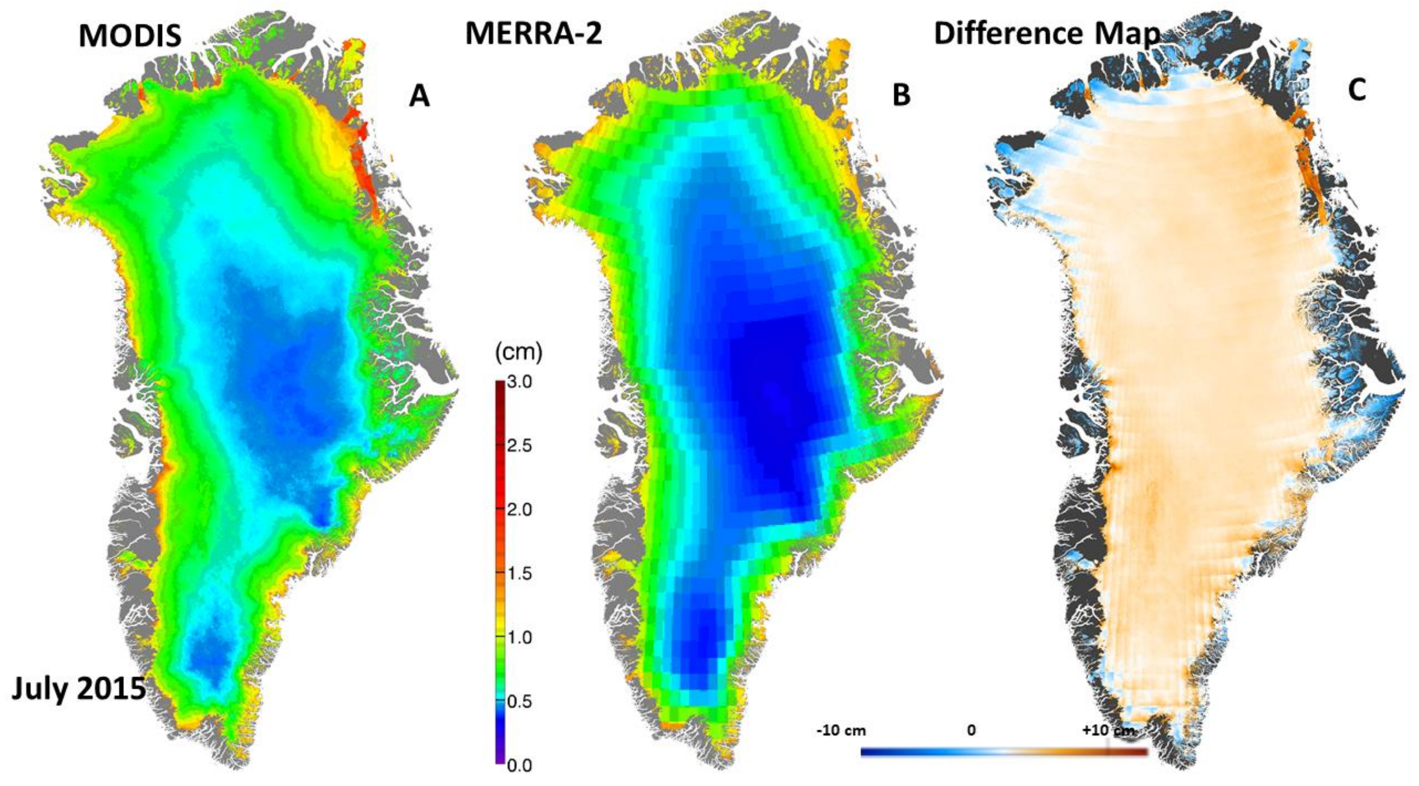
6. Comparisons with Modern Era Retrospective Analysis for Research and Applications, Version 2 (MERRA-2)

Although we cannot validate the MODIS albedo and WV layers of the multilayer product using in situ data, we can perform comparisons with modeled data such as from Modern Era Retrospective analysis for Research and Applications, Version 2 (MERRA-2). Such comparisons using other satellite data have already been undertaken [31]. MERRA-2 is the latest atmospheric reanalysis of the modern satellite era produced by NASA’s Global Modeling and Assimilation Office [https://gmao.gsfc.nasa.gov/reanalysis/MERRA–2/], including a representation of ice sheets over Greenland and Antarctica. The inherent spatial resolution is 1/2° latitude × 5/8° longitude [32].

After regridding the MERRA-2 data to the ~0.78 km polar stereographic grid, we compared MODIS albedo and WV maps from the ESDR with maps developed from MERRA-2 output. We also use in situ data and the MODIS IST to provide validation of the MERRA-2 skin temperatures because the MODIS IST is accurate to ≤±1.3 °C under clear skies, as described earlier.

To illustrate a method for validation of MERRA-2 skin temperature, we show comparisons between MODIS IST from the ESDR and MERRA-2 skin temperatures using monthly MODIS IST and MERRA-2 maps for January and July of 2015. The three maps in the top panel in Figure 11 show the MODIS IST monthly product for January of 2015 (A), the MERRA-2 mean monthly skin temperature (B), and the difference map (C). In the bottom panel, the MODIS monthly product (D) is the same as (A), but the MERRA-2 monthly skin temperature map (E) was developed using only MERRA-2 hourly data that matched the times of the MODIS swaths that were used to create the MODIS monthly map shown in (A) and (D), so the comparison is more valid than when all of the MERRA-2 hourly data are used to create the MERRA-2 mean monthly map as in the top panel. The agreement between the MODIS and MERRA-2 maps increased from R = 0.90 for panels (A) and (B) to R = 0.94 for panels (D) and (E) when MERRA-2 hourly data were selected to match the times of the MODIS swaths. Only ice sheet cells were used to create the maps, where N = 2,867,800. Land in the coastal areas of Greenland was excluded.

In Figure 12, the MERRA-2 skin temperature map for July 2015 (B) was developed using values selected to match the times of the MODIS swath acquisitions that were used to create the MODIS monthly map (A); the difference map (MODIS IST minus MERRA-2) is shown in (C). For this comparison, the agreement between the MODIS and MERRA-2 maps in panels (A) and (B) is R = 0.91, and N = 2,867,800.

Comparing MODIS IST and MERRA-2 skin temperature data from individual days, we selected days that were relatively cloud-free on the MODIS maps, to maximize the number of cloud-free grid cells to compare. As an example, in Figure 13, the MERRA-2 skin temperature map for 4 January 2015 (B) was developed using hourly data to match the times of the MODIS swaths acquired on the same day as shown in (A) in the top row, yielding an agreement of R = 0.93, where N = 2,429,937.

To provide some validation of the MERRA-2 hourly skin temperatures, we also compared daily skin temperature from MERRA-2 with daily skin temperature derived in situ from the Adolph et al. [29] study site north-northwest of Summit for the 40 day study period (Figure 14). All of the in situ data were averaged for each day and all of the hourly MERRA-2 skin temperature data were averaged for each 24 h period for this comparison. The agreement was R = 0.92, with an RMSE of 2.86 °C, where N = 40.

Monthly MODIS broadband albedo and the monthly mean broadband albedo from MERRA-2 and a difference map (MODIS minus MERRA-2) are shown in Figure 15. To calculate the MODIS monthly albedo, daily albedo values were used since there are no swath-based albedo data products from MODIS, MOD10A1. However, hourly broadband albedo values were used to calculate the monthly mean albedo from MERRA-2. The correlation is R = 0.74, and N = 2,867,800.

For 1 July 2015, the MODIS daily albedo and MERRA-2 albedo are shown along with a difference map for that day, in Figure 16. To calculate the MERRA-2 albedo, we averaged all of the data for the 24 h period, provided in the MERRA-2 dataset, to compare with the daily MODIS albedo map from the ESDR. The correlation between the MODIS daily albedo and the MERRA-2 daily albedo was R = 0.65. Only ice sheet cells that were cloud-free on MODIS were used to create the maps, where N = 1,978,312.

For the month of July 2015, we show the monthly mean MODIS WV, the monthly mean MERRA-2 WV, and a WV difference (MODIS minus MERRA-2) map in Figure 17. Note the small differences in WV for the MODIS and MERRA-2 WV maps for the month of July 2015, where R = 0.90. The number of cells available to create the maps is N = 2,868,630.

7. Discussion and Conclusions

A multilayer IST, albedo, and water vapor MODIS-based ESDR of the Greenland Ice Sheet, extending from March 2000 through December 2016, was developed to facilitate studies of complex geophysical relationships and to meet the needs of the ice sheet modeling community. The new ESDR provides Collection 6.1 Terra MODIS IST and surface melt and Collection 6 albedo and water vapor, as well as ancillary information, in a polar stereographic projection with ~0.78 km resolution in NetCDF.

Validation of the IST at the swath level has been conducted using in situ and aircraft data for selected parts of the ice sheet. Earlier results show that the IST algorithm is accurate to ≤±1.3 °C under clear-sky conditions (for example, see [6,30]). The IST in the new ESDR can be used to validate reanalysis data such as from MERRA-2. For the albedo and water vapor maps within the ESDR, in situ absolute “ground truth” measurements are not available; however, the ESDR can be compared with maps developed from MERRA-2 and other reanalysis products.

Confidence in trends discovered in remotely sensed datasets increases when results are attained independently (e.g., see [33,34]), or when different datasets are used to produce a similar result. In previously published work, calculated trends of albedo during the period of the MODIS record have been shown to be affected by algorithm changes related to reprocessing of MODIS data products. For example, using C5 data, a strongly declining albedo trend calculated using MOD10A1 was shown by Casey et al. [21] to be erroneous when MOD10A1 C6 data, with corrections for sensor degradation included, was used.

The MOD29 IST algorithm is derived from an algorithm originally developed by Key et al. [35] and modified for MODIS [6]. This same basic algorithm is in use for the Suomi-NPP Visible Infrared Imaging Radiometer Suite (VIIRS) IST product [36]. The decision to use IST for the new ESDR was made to facilitate the development of an intersatellite ESDR and ultimately a moderate-resolution climate data record (CDR) beginning with MODIS data in 2000 and continuing through the VIIRS era. A second VIIRS instrument was launched on 18 November 2017 on the Joint Polar Satellite System-1 (JPSS-1), and additional VIIRS instruments are planned for launch in the future on the JPSS-2 and -3 satellites, thus potentially extending the record.

Use of consistent algorithms is important for the study of long-term changes in the skin temperature, surface melt, albedo, and water vapor of the Greenland Ice Sheet. Because of inherent uncertainties of all datasets and, in particular, with time series data sets involving cloud masking, it is highly advantageous to use a combination of in situ and/or products from different satellites and sensors, to identify trends in geophysical features such as IST, albedo, and water. Reliance on any one dataset, alone, could be problematic.

This ESDR will be available through the National Snow and Ice Data Center in the summer of 2018: https://doi.10.5067/7THUWT9NMPDK.

References

1. Enderlin, E.M.; Howat, I.M.; Jeong, S.; Noh, M.-J.; Angelen, J.H.; Broeke, M.R. An improved mass budget for the Greenland ice sheet. Geophys. Res. Lett. 2014, 41, 866–872. [Google Scholar] [CrossRef]
2. Price, S.F.; Payne, A.G.; Howat, I.M.; Smith, B.E. Committed sea-level rise for the next century from Greenland ice sheet dynamics during the past decade. Proc. Natl. Acad. Sci. USA 2011, 108, 8978–8983. [Google Scholar] [CrossRef] [PubMed]
3. Nowicki, S.; Bindschadler, R.A.; Abe-Ouchi, A.; Aschwanden, A.; Bueler, E.; Choi, H.; Fastook, J.; Granzow, G.; Greve, R.; Gutowski, G.; et al. Insights into spatial sensitivities of ice mass response to environmental change from the SeaRISE ice sheet modeling project II: Greenland. J. Geophys. Res. 2013, 118, 1002–1024. [Google Scholar] [CrossRef]
4. Cullather, R.I.; Nowicki, S.M.J.; Zhao, B.; Suarez, M.J. Evaluation of the surface representation of the Greenland ice sheet in a general circulation model. J. Clim. 2014, 27, 4835–4856. [Google Scholar] [CrossRef]
5. Hall, D.K.; Comiso, J.C.; DiGirolamo, N.E.; Shuman, C.A.; Key, J.; Koenig, L.S. A Satellite-Derived Climate-Quality Data Record of the Clear-Sky Surface Temperature of the Greenland Ice Sheet. J. Clim. 2012, 25, 4785–4798. [Google Scholar] [CrossRef]
6. Hall, D.K.; Key, J.; Casey, K.A.; Riggs, G.A.; Cavalieri, D.J. Sea ice surface temperature product from the Moderate-Resolution Imaging Spectroradiometer (MODIS). IEEE Trans. Geosci. Remote Sens. 2004, 42, 1076–1087. [Google Scholar] [CrossRef]
7. Howat, I.M.; Negrete, A.; Smith, B.E. The Greenland Ice Mapping Project (GIMP) land classification and surface elevation data sets. Cryosphere 2014, 8, 1509–1518. [Google Scholar] [CrossRef]
8. Zwally, H.J.; Giovinetto, M.B.; Beckley, M.A.; Saba, J.L. Antarctic and Greenland Drainage Systems; GSFC Cryospheric Sciences Laboratory: Washington, DC, USA, 2012. [Google Scholar]
9. Moeller, C.; Frey, R. Terra MODIS Collection 6.1 Calibration and Cloud Product Changes. 2017. Available online: https://modis-atmosphere.gsfc.nasa.gov/sites/default/files/ModAtmo/C6.1_Calibration_and_Cloud_Product_Changes_UW_frey_CCM_1.pdf (accessed on 9 January 2018).
10. Riggs, G.A.; Hall, D.K.; Salomonson, V.V. MODIS Sea Ice Products User Guide; The College of Information Sciences and Technology: University Park, PA, USA, 2006. [Google Scholar]
11. Klein, A.G.; Stroeve, J. Development and validation of a snow albedo algorithm for the MODIS instrument. Ann. Glaciol. 2002, 34, 45–52. [Google Scholar] [CrossRef]
12. Stroeve, J.C.; Box, J.E.; Haran, T. Evaluation of the MODIS (MOD10A1) daily snow albedo product over the Greenland ice sheet. Remote Sens. Environ. 2006, 105, 155–171. [Google Scholar] [CrossRef]
13. Box, J.E.; Fettweis, X.; Stroeve, J.C.; Tedesco, M.; Hall, D.K.; Steffen, K. Greenland ice sheet albedo feedback: Thermodynamics and atmospheric drivers. Cryosphere 2012, 6, 1–19. [Google Scholar] [CrossRef]
14. Brun, F.; Dumont, M.; Wagnon, P.; Berthier, E.; Azam, M.F.; Shea, J.M.; Sirguey, P.; Rabatel, A.; Ramanathan, A. Seasonal changes in surface albedo of Himalayan glaciers from MODIS data and links with the annual mass balance. Cryosphere 2015, 9, 341–355. [Google Scholar] [CrossRef]
15. Burakowski, E.A.; Ollinger, S.V.; Lepine, L.; Schaaf, C.B.; Wang, Z.; Dibb, J.E.; Hollinger, D.H.; Kim, J.; Erb, A.; Martin, M. Spatial scaling of reflectance and surface albedo over a mixed-use, temperate forest landscape during snow-covered periods. Remote Sens. Environ. 2015, 158, 465–477. [Google Scholar] [CrossRef]
16. Tedesco, M.; Doherty, S.; Fettweis, X.; Alexander, P.; Jeyaratnam, J.; Stroeve, J. The darkening of the Greenland ice sheet: Trends, drivers, and projections (1981–2100). Cryosphere 2016, 10, 477–496. [Google Scholar] [CrossRef]
17. Moustafa, S.E.; Rennermalm, A.K.; Román, M.O.; Wang, Z.; Schaaf, C.B.; Smith, L.; Koenig, L.S.; Erb, A. Evaluation of satellite remote sensing albedo retrievals over the ablation area of the southwestern Greenland ice sheet. Remote Sens. Environ. 2017, 198, 115–125. [Google Scholar] [CrossRef]
18. Gao, B.-C.; Kaufman, Y.J. Water vapor retrievals using Moderate Resolution Imaging Spectroradiometer (MODIS) near-infrared channels. J. Geophys. Res. 2003, 108, 4389–4398. [Google Scholar] [CrossRef]
19. Toller, G.; Xiong, X.; Sun, J.; Wenny, B.; Geng, X.; Kuyper, J.; Angal, A.; Chen, H.; Madhavan, S.; Wu, A. Terra and Aqua moderate-resolution imaging spectroradiometer collection 6 level 1B algorithm. J. Appl. Remote Sens. 2013, 7, 073557. [Google Scholar] [CrossRef]
20. Polashenski, C.M.; Dibb, J.E.; Flanner, M.G.; Chen, J.Y.; Courville, Z.R.; Lai, A.M.; Schauer, J.J.; Shafer, M.M.; Bergin, M. Neither dust nor black carbon causing apparent albedo decline in Greenland’s dry snow zone: Implications for MODIS C5 surface reflectance. Geophys. Res. Lett. 2015, 42, 9319–9327. [Google Scholar] [CrossRef]
21. Casey, K.; Polashenski, C.M.; Chen, J.; Tedesco, M. Impact of MODIS sensor calibration updates on Greenland ice sheet surface reflectance and albedo trends. Cryosphere 2017, 11, 1781–1795. [Google Scholar] [CrossRef]
22. Hall, D.K.; Comiso, J.C.; DiGirolamo, N.E.; Shuman, C.A.; Box, J.; Koenig, L.S. Variability in the surface temperature and melt extent of the Greenland ice sheet from MODIS. Geophys. Res. Lett. 2013, 40, 1–7. [Google Scholar] [CrossRef]
23. Wenny, B.; Wu, A.; Madhavan, S.; Wang, Z.; Li, Y.; Chen, N.; Chiang, K.-F.; Xiong, X. MODIS TEB calibration approach in Collection 6. In Proceedings of the Sensors, Systems, and Next-Generation Satellites XVI, Edinburgh, UK, 24–27 September 2012. [Google Scholar]
24. Wu, A.; Wang, Z.; Li, Y.; Madhavan, S.; Wenny, B.; Chen, N.; Xiong, X. Adjusting Aqua MODIS TEB nonlinear calibration coefficients using iterative solution. In Proceedings of the Earth Observing Missions and Sensors: Development, Implementation, and Characterization III, Beijing, China, 13–16 October 2014. [Google Scholar]
25. Wilson, T.; Wu, A.; Shrestha, A.; Geng, X.; Wang, Z.; Moeller, C.; Frey, R.; Xiong, X. Development and Implementation of an Electronic Crosstalk Correction for Bands 27–30 in Terra MODIS Collection 6. Remote Sens. 2017, 9, 569. [Google Scholar] [CrossRef]
26. Mortimer, C.A.; Sharp, M. Characterization of Canadian High Arctic glacier surface albedo from MODIS C6 data, 2001–2016. Cryosphere 2018, 12, 701–720. [Google Scholar] [CrossRef]
27. Shuman, C.A.; Hall, D.K.; DiGirolamo, N.E.; Mefford, T.K.; Schnaubelt, M.J. Comparison of near-surface air temperatures and MODIS ice-surface temperatures at Summit, Greenland (2008–2013). J. Appl. Meteorol. Climatol. 2014, 53, 2171–2180. [Google Scholar] [CrossRef]
28. Ryan, J.C.; Hubbard, A.; Irvine-Fynn, T.D.; Doyle, S.H.; Cook, J.M.; Stibal, M.; Box, J.S. How robust are in-situ observations for validating satellite-derived albedo over the dark zone of the Greenland Ice Sheet? Geophys. Res. Lett. 2017, 44, 6218–6225. [Google Scholar] [CrossRef]
29. Adolph, A.; Albert, M.R.; Hall, D.K. Near-surface thermal stratification during summer at Summit, Greenland, and its relation to MODIS-derived surface temperatures. Cryosphere 2018, 12, 907–920. [Google Scholar] [CrossRef]
30. Hall, D.K.; Nghiem, S.V.; Rigor, I.G.; Miller, J.A. Uncertainties of temperature measurements on snow-covered land and sea ice from in-situ and MODIS data during BROMEX. J. Appl. Meteorol. Climatol. 2015, 54, 966–978. [Google Scholar] [CrossRef]
31. Eyre, J.J.R.; Zeng, X. Evaluation of Greenland near surface air temperature datasets. Cryosphere 2017, 11, 1591–1605. [Google Scholar] [CrossRef]
32. Gelaro, R.; McCarty, W.; Suarez, M.; Todling, R.; Molod, A.; Takacs, L.; Randles, C. The Modern-Era Retrospective Analysis for Research and Applications, Version 2 (MERRA-2). J. Clim. 2017, 30, 5419–5454. [Google Scholar] [CrossRef]
33. Comiso, J.C. Warming trends in the Arctic. J. Clim. 2003, 16, 3498–3510. [Google Scholar] [CrossRef]
34. Wang, X.; Key, J.R. Recent trends in Arctic surface, cloud, and radiation properties from space. Science 2003, 299, 1725–1728. [Google Scholar] [CrossRef] [PubMed]
35. Key, J.; Collins, C.; Fowler, C.; Stone, R.S. High-latitude surface temperature estimates from thermal satellite data. Remote Sens. Environ. 1997, 61, 302–309. [Google Scholar] [CrossRef]
36. Tschudi, M.; Riggs, G.A.; Hall, D.K.; Román, M.O. NASA S-NPP VIIRS Ice Surface Temperature Collection 1 User Guide; National Aeronautics and Space Administration: Washington, DC, USA, 2016. [Google Scholar]
Figure 1. Examples of monthly ice surface temperature (IST) maps of the Greenland Ice Sheet derived from the Collection 6.1 MOD29 special IST product for Greenland, for June through September 2015.
Remotesensing 10 00555 g001
Figure 2. Examples of monthly surface melt maps of the Greenland Ice Sheet derived from the MOD29 special MODerate-resolution Imaging Spectroradiometer (MODIS) ice surface temperature product, for June through September 2015.
Remotesensing 10 00555 g002
Figure 3. Maps of maximum annual surface melt on the Greenland Ice Sheet derived from the MOD29 MODIS monthly ice surface temperature (IST) product of Greenland (2000–2016).
Remotesensing 10 00555 g003
Figure 4. Examples of the monthly snow albedo maps of the Greenland Ice Sheet derived from the Collection 6 MOD10A1 standard MODIS product, for June through September 2015.
Remotesensing 10 00555 g004
Figure 5. Examples of monthly water vapor maps of the Greenland Ice Sheet derived from the Collection 6 MOD05 standard MODIS product [18], for June through September 2015.
Remotesensing 10 00555 g005
Figure 6. Eight major drainage basins of the Greenland Ice Sheet [7].
Remotesensing 10 00555 g006
Figure 7. (Left) Map from the earlier ice surface temperature (IST) Earth Science Data Record (ESDR) that used MODIS Collection 5 IST data from MOD29. (Right) Map from the new ESDR, using MOD29 Collection 6.1 data. Note the more detailed land/water/ice mask and the fewer cloud pixels in the new IST map.
Remotesensing 10 00555 g007
Figure 8. Four-day composites from 10–13 July 2014 of the daily ice surface temperature (IST), surface melt, albedo, and water vapor (WV) maps. Coastal land outside of the ice sheet is dark green and cloud is grey; missing data is black. The red arrow points to the same place on each map. Cloud cover is different on the IST, melt, and albedo maps because of the way the algorithms perform the compositing even though the maps are derived from the same four-day period.
Remotesensing 10 00555 g008
Figure 9. Skin temperature from Adolph et al. [29] versus ice surface temperature from the new ESDR at the study site north-northwest of Summit Station (72.65923°N, -38.57067°W) for the 40 day study period, 8 June−18 July 2015.
Remotesensing 10 00555 g009
Figure 10. Comparison of ice surface temperature (IST) and KT-19 infrared-radiometer-derived temperature acquired during IceBridge flights over Greenland between 13 March and 21 May 2014. The points shown in red are derived from a flight segment on 29 April which was a day with minimal cloud cover (though was not completely cloud-free).
Remotesensing 10 00555 g010
Figure 11. January 2015 monthly maps. Top row: Monthly average of all available data. (A): MODIS ice surface temperature (IST) swath; (B): Modern Era Retrospective analysis for Research and Applications, Version 2 (MERRA-2) skin temperature; (C): MODIS minus MERRA-2 difference map, in °C, for January 2015. Bottom row: (D): Monthly average of all available MODIS IST swath data as in (A); (E): MERRA-2 skin temperatures averaged over times corresponding to available MODIS IST swaths used to create (A,D); and (F): difference map, in °C, of MODIS minus MERRA-2, for January 2015.
Remotesensing 10 00555 g011
Figure 12. July 2015 monthly maps. (A): MODIS daily ice surface temperature in °C, for July 2015; (B): MERRA-2 monthly temperatures in °C for July 2015 where MERRA-2 hourly skin temperature data were selected to match times corresponding to the MODIS swaths and then averaged to create a monthly map; (C): MODIS minus MERRA-2 difference map, in °C. The agreement between the MODIS and MERRA-2 maps in panels (A,B) is R = 0.91, and N = 2,867,800.
Remotesensing 10 00555 g012
Figure 13. 4 January 2015 skin temperature maps. (A): MODIS daily ice surface temperature (IST); (B): MERRA-2 skin temperature averaged from times selected to correspond to available MODIS IST swaths used to develop (A); and (C): a difference map, in °C, of MODIS minus MERRA-2, for 4 January 2015. Note in (B) that black on the MERRA-2 map shows where clouds are found in the MODIS map.
Remotesensing 10 00555 g013
Figure 14. Skin temperature from Adolph et al. [29] vs MERRA-2 skin temperature at the study site north-northwest of Summit Station (72.65923°N, −38.57067°W) for the 40 day study period, 8 June–18 July 2015. The agreement was R = 0.92, with an RMSE of 2.86 °C, where N = 40.
Remotesensing 10 00555 g014
Figure 15. Comparison of MODIS and MERRA-2 mean monthly albedo for July 2015. The left panel shows the monthly MODIS albedo, the center panel shows the mean monthly MERRA-2 albedo and the panel on the right shows the difference map (MODIS minus MERRA-2). The correlation is R = 0.74, and N = 2,867,800.
Remotesensing 10 00555 g015
Figure 16. Comparison of MODIS and MERRA-2 daily albedo for 1 July 2015. (A): Daily MODIS albedo, (B): daily MERRA-2 albedo, and (C): difference map (MODIS minus MERRA-2). The correlation between the MODIS daily albedo and the MERRA-2 daily albedo is R = 0.65. Only ice sheet cells that were cloud-free on MODIS were used to create the maps, where N = 1,978,312.
Remotesensing 10 00555 g016
Figure 17. Comparison of MODIS and MERRA-2 monthly mean water vapor for July 2015. (A): Monthly MODIS WV, (B): Monthly MERRA-2 WV, and (C): difference map (MODIS minus MERRA-2). This comparison yields a correlation of R = 0.90; the number of cells available to create the maps is N = 2,868,630.
Remotesensing 10 00555 g017