Implementation of the LandTrendr Algorithm on Google Earth Engine

Abstract

The LandTrendr (LT) algorithm has been used widely for analysis of change in Landsat spectral time series data, but requires significant pre-processing, data management, and computational resources, and is only accessible to the community in a proprietary programming language (IDL). Here, we introduce LT for the Google Earth Engine (GEE) platform. The GEE platform simplifies pre-processing steps, allowing focus on the translation of the core temporal segmentation algorithm. Temporal segmentation involved a series of repeated random access calls to each pixel’s time series, resulting in a set of breakpoints (“vertices”) that bound straight-line segments. The translation of the algorithm into GEE included both transliteration and code analysis, resulting in improvement and logic error fixes. At six study areas representing diverse land cover types across the U.S., we conducted a direct comparison of the new LT-GEE code against the heritage code (LT-IDL). The algorithms agreed in most cases, and where disagreements occurred, they were largely attributable to logic error fixes in the code translation process. The practical impact of these changes is minimal, as shown by an example of forest disturbance mapping. We conclude that the LT-GEE algorithm represents a faithful translation of the LT code into a platform easily accessible by the broader user community.

1. Introduction

After the opening of the Landsat image archive in 2008 [1], time series analysis of Landsat imagery has blossomed, with rapid development of new algorithms and capabilities for change detection [2]. The LandTrendr (Landsat-based detection of trends in disturbance and recovery) algorithm was among the first wave of such approaches [3], using temporal segmentation of spectral trajectories as a means of distilling and extracting meaningful change information from the rich Landsat archive [4]. Although used in a variety of applications by the developers [5,6,7,8] and adopted by other labs [9,10,11,12], the broader utility of the LandTrendr (LT) algorithm to the community was dampened by key obstacles. First, the code was written in a proprietary processing language (IDL; ITTVis Incorporated), whose cost and learning curve were impediments to accessibility. Second, its workflow to build time-series image stacks required significant person-time investment in image pre-processing and data management before the algorithm could be run. Finally, running the algorithm itself required much computing time, often two to three days for a single Landsat scene on a typical machine. Combined, these obstacles limited the algorithm to users with substantial computational resources and remote sensing expertise. Even for those users, the costs involved in acquiring and managing data severely limited the experimentation, exploration, and expansion of the algorithm in new domains.

To enhance benefits to the broader community, we introduce LT for the Google Earth Engine (GEE) platform. GEE is attractive not only because of its free access, but also because of its broad and growing user base, full access to the Landsat archive, straightforward management of time series stacks, and ease of parallel processing to speed computation [13]. However, translation of any science code to a cloud-based, scaled production environment requires careful evaluation of original code and may require modifications of code structure. Thus, we describe key decisions and findings in translating the original IDL-based LT code (hereafter LT-IDL) into an equivalent algorithm on GEE (hereafter LT-GEE) and report on simple tests to ensure fidelity of the LT-GEE implementation. Implementing a familiar but complex desktop-based algorithm in a parallel processing environment, especially when access to thousands of images is required, is far from a straightforward task. We use this technical note to document programming logic and validation results for such a reinvention of the LT algorithm.

2. Materials and Methods

2.1. Background on Code and Platform

Although the LT algorithm and the GEE platform have been amply described elsewhere, we provide a brief overview here of the key characteristics of each that affected translation of the algorithm.

The overarching goal of LT is to characterize a temporal trajectory of data values using a sequence of connected linear segments bounded by nodes or break-points referred to here as “vertices”. The incoming data values can be spectral bands, derived spectral indices, or even other metrics that themselves capture yearly behavior (such as maximums of an index, etc.). The only constraint is that there can be one value per year. Two phases are used to find vertices. In a forward phase, candidate vertices are identified through an iterative anomaly detection criterion, and in a reverse phase those candidate vertices are culled using an angle-of-change criterion. Once a user-defined maximum number of vertices is identified, straight-line segments are fit to the observed spectral metric values, working from the first year in the time series to the last. Fitting uses either simple regression or point-to-point fitting, constrained to ensure that the starting vertex of a subsequent segment is anchored to the ending vertex of the prior segment. From this best-fitting model with the maximum number of vertices, an iterative process of vertex-removal and re-fitting is conducted to find successively simpler renditions of the time series. At each step in the iteration, goodness of fit statistics are calculated that penalize more complex fits, and fitting statistics are compared against a user-defined threshold. If none of the renditions of the time series meet that threshold, an entirely separate fitting approach is invoked that uses a Levenburg-Marquardt optimization to fit all vertices simultaneously. Finally, from these successively simpler renditions of the time series, the best model is chosen based on the best fitting statistic, with a user-defined parameter allowing more complex fits to be chosen if they are within a user-defined proportion of the best fit statistic. The IDL-version of the algorithm is available at https://github.com/KennedyResearch/LandTrendr-2012.

Three categories of pre-processing are needed before segmentation can occur. The first is the typical preprocessing of the imagery itself: geometric rectification, cloud and shadow screening, and calculation of surface reflectance or some similar metric to ensure consistency across time. Second, a single data value per year must be identified; this can be done using rules for best-pixel identification or through a derived metric (such as median spectral value across multiple dates; maximum value within a season, etc.). After these two generic categories of pre-processing are complete, pixel level time-series of data values are passed to the LT algorithm, in which two internal pre-processing steps are applied. The first is a despiking algorithm controlled by a user-defined parameter to dampen sporadic anomalies. The second involves missing data. When appropriate pixel values are not available in a given year because of cloud cover or gaps in the data archive, these can be flagged as missing and ignored in the vertex-seeking phase of the algorithm; they then become filled in with spectral values once segments are constructed using good values from before or after.

As a cloud-based geoprocessing platform designed to provide computational access to vast geospatial datasets, Google Earth Engine is an excellent choice to implement an algorithm such as LT [13]. With a powerful application programming interface (API) built on top of an analysis-ready catalog of many multitemporal datasets, including more than 7 million Landsat images, GEE condenses many previously onerous steps to a few lines of code. Of particular relevance to LT is ready access to the surface reflectance archives of Landsat Thematic Mapper (TM/ETM+) and Operational Land Imager (OLI) imagery, as well as associated cloud and shadow masks developed using standard protocols [14]. Additionally, the GEE data construct of “image collections” allows simple creation of image time series with sophisticated image selection and screening criteria, and it simplifies parallel processing. Finally, the GEE interface allows sharing of scripts among researchers.

2.2. Integration of LT into GEE

The LT algorithm is data intensive and relies heavily on repeated random access into the time series. The input for each pixel is the annual time series of one spectral band or index, plus the date for each of those observations, and computing the vertices involves generating multiple models that include different groupings of the input values. To make this efficient in the parallel processing architecture offered by Earth Engine, the algorithm was converted to Java and modified to operate on the time series of one pixel at a time. The backend efficiently handles applying the algorithm independently to each time series stack of pixels in a region, using the tile-based data distribution model outlined in Gorelick et al. [13].

Because the outputs of LT are of variable length by nature (varying with the number of input time steps at each pixel location), the outputs are generated as a 2-D array and the segmentation RMSE per pixel. This array contains four output rows: the original time and spectral values used to identify vertices, the spectral values fitted using the identified vertices, and a Boolean for each time value indicating if the value was determined to be a vertex. Additionally, if more than one band was supplied as input, all bands beyond the first one are also fitted using the identified set of vertices.

Translation required slight modifications to the logic of the original code. To aid in the debugging and validation, the algorithm was first transliterated from the IDL implementation as closely as possible. Once completed and validated, the code underwent restructuring optimizations to minimize overall memory usage and heap allocations. Statistical fitting rules were translated to underlying GEE statistical libraries, with possible slight improvements in floating-point precision. Additionally, during IDL code scrutiny, two logic errors were identified and corrected. First, the de-spiking algorithm in the original code had been erroneously applied to all time series, even if no significant spikes were present. Second, the application of fitting rules to optional additional spectral bands did not appropriately apply the Levenburg-Marquardt fitting rules when the early-to-late sequential fitting failed.

2.3. Testing LT-GEE vs. LT-IDL

To compare the LT-IDL and LT-GEE algorithms, we developed tests to evaluate segmentation outputs while holding as many factors consistent as possible. The overall workflow was thus to develop standard image datasets in GEE, process those identical image stacks using LT-IDL and LT-GEE, and then evaluate agreement of vertices and overall fitting (Figure 1).

2.3.1. Study Areas

To conduct our tests, we selected six equal-sized, square study areas (~184 by 184 km) in the continental United States (Figure 2). Most of our study regions include substantial forest [15], as the primary focus of LT-IDL to date has been on forest dynamics, but we also chose to include two study areas with minimal forest cover to explore algorithm behavior in temporally variable systems.

2.3.2. Image Collections

We used GEE to build stacks of Landsat Thematic Mapper (TM), Enhanced Thematic Mapper + (ETM+), and Operational Land Imager (OLI) spectral metrics for the period 1984 to 2016 as inputs to the LT algorithms. Image collections were constrained to the date range from 20 June to 10 September; we used Landsat data from the Pre-Collection 1 archive to maintain consistency with prior reporting on our LT-IDL algorithm. LT requires that each pixel contain only a single spectral value for each pixel in each year. We used a medoid selection process, in which each pixel’s six-band (the optical wavelengths of TM and ETM+ and equivalent bands from OLI) spectral values were compared to the median six-band spectral values of that pixel in all images in that year’s date-constrained collection, and the spectral values from the pixel closest to that median value (using Euclidean spectral distance) were chosen. We then calculated for each chosen pixel the normalized burn ratio (NBR: [NIR−SWIR2]/[SWIR2+NIR]; [16]) to build the pixel-level time series. This was repeated for all pixels in our study areas to create stacks of NBR as input to the algorithms.

2.3.3. Algorithms

Image NBR stacks were either submitted directly to the LT-GEE segmentation algorithm in the GEE User-interface or exported to Google Drive and downloaded to run the LT-IDL segmentation algorithm on a local server. For the latter, we then assigned file names and metadata to match the format expected by the LT-IDL routines. The LT algorithms were run with equivalent parameters; when a parameter was dropped in the LT-GEE version, we set it to a value that would disable it in the LT-IDL run (

Table 1. LandTrendr parameters used for IDL and GEE runs in all study areas. The NBR spectral metric was used for segmentation. For descriptions of the parameters, see [3]).

Parameter	IDL	GEE	Comments
maxSegments	6	6
spikeThreshold	0.9	0.9	Renamed from “desawtooth val”
vertexCountOvershoot	3	3
recoveryThreshold	0.25	0.25
pvalThreshold	0.05	0.05
bestModelProportion	0.75	0.75
minObservationsNeeded	6	6	Renamed from “minneeded”
Background_val	0	NA	GEE uses a mask logic to avoid missing values caused by clouds, shadows, and missing imagery.
Divisor	−1	NA	Ensures that vegetation loss disturbance results in negative change in value when NBR is used as a spectral metric. In GEE, this must be handled outside of the segmentation algorithm.
Kernelsize	1	Dropped	Originally used together with skipfactor to save computational burden; no longer necessary.
Skipfactor	1	Dropped
Distweightfactor	2	Dropped	Inadvertently hardwired in the IDL code, this parameter was hardwired in the GEE code to the value of 2.
Fix_doy_effect	1	Dropped	Although correcting day-of-year trends was considered theoretically useful in the original LT implementation, in practice it has been found to distort time series values when change occurs and thus was eliminated.

).

2.3.4. Evaluation

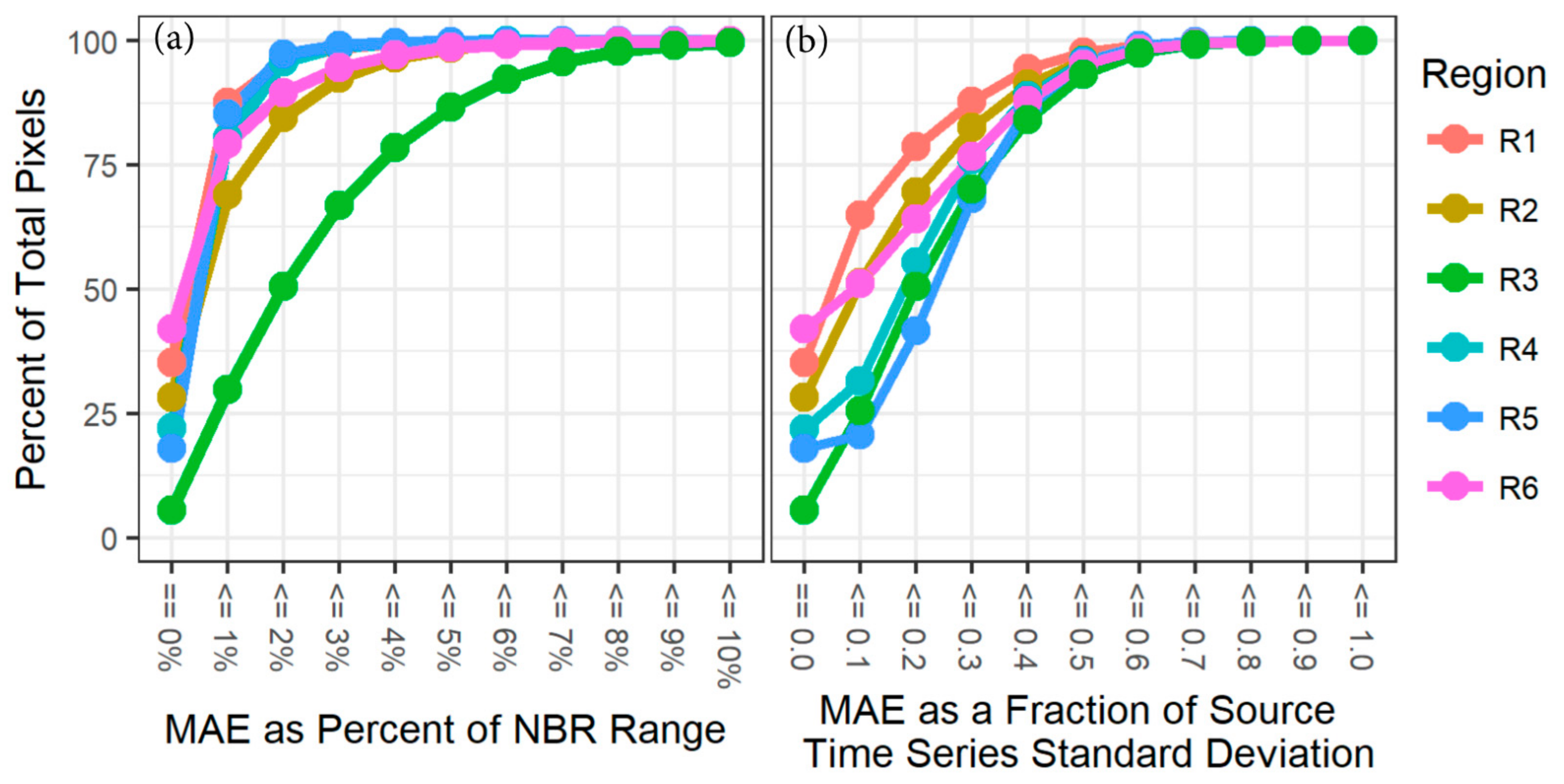
We compared outputs from the LT segmentation process run using LT-IDL against those from LT-GEE. As noted above, outputs from the pixel-level LT segmentation process include both original yearly spectral values, fitted spectral values, and a Boolean indicator to identify vertices. We used two metrics to compare results: (1) Difference in vertex count and (2) Mean absolute error (MAE), calculated as the mean across years of the absolute value of fitted NBR from LT-IDL minus LT-GEE. The former provides a simple estimate of the complexity of the segmentation found by each algorithm, while the latter measures that pragmatic impact of any differences in the fit. We used cumulative distributions of MAE scaled two different ways to facilitate visual comparison among regions. The first scaling was simply relative to overall NBR range (−1.0 to 1.0), providing a sense of the absolute impact of the error. In the second scaling approach, we compared MAE relative to the standard deviation of the original time series spectral values (i.e., before segmentation). This provides a per-pixel sense of the relative impact of differences in fitting.

3. Results

In all six study regions, LT-GEE and LT-IDL agreed on the number of segmentation vertices in the majority of pixels, and where they disagreed, the disagreement was largely balanced between the two algorithms (Figure 3). The exception is Region 5, in which the LT-GEE version of the algorithm consistently found more vertices than the LT-IDL version did. We discuss possible explanations below.

Mean absolute error showed high agreement between the two versions of the algorithm, with the vast majority of pixels showing an MAE difference of less than 3% of the range of NBR for five of six study regions (Figure 4a). The one exception is in Region 3, an agriculturally dominated system that we discuss below. Rescaling MAE to the per-pixel standard deviation of spectral signal, the accumulated error was more consistent across regions, with the more heavily forested regions (R1, R2, R6) showing better agreement than the agricultural and drier regions (R3, R4, R5).

4. Discussion

Before discussing the specifics of the code translation and testing, it is important to note the realized benefits to the user of utilizing GEE for implementation of LT. The first is simply the vast reduction in data handling and management cost: to process and handle imagery for six study areas across the U.S., we would have typically budgeted several weeks of person time to the simple process of image selection, downloading, management, and alignment of the data. With LT-GEE, such time investment diminishes to essentially zero, and new sites can be added by simple addition of a line or two of code. Scaling up to arbitrary spatial scales also requires none of the additional data storage costs that would otherwise be needed. Second, actual computational cost and time to completion are also reduced to being almost trivial: using the LT-IDL algorithm in the past, temporal segmentation of each site would have taken close to three days of compute time; utilizing the distributed cloud computing capacities of LT-GEE, each site completes in 20–40 min. These benefits not only serve to lower barriers to entry, they also allow “power users” in the remote sensing community to explore and evaluate different approaches to running the algorithm. For example, with LT-GEE it is trivial to investigate the impact of changing the date window on which image stacks are built; in the past, decision of date windows was major management choice that affected all subsequent work flows. Similarly, costs of processing and data management limited our past explorations of the impact and information content of using different spectral indices; with the LT-GEE implementation, it is possible to design studies that exhaustively explore the information content of the data space [17]. The adaptation of LT-IDL to LT-GEE represents the current reality in the field of remote sensing: advances come from the confluence of data, computation, and algorithms. Moreover, implementation in GEE makes algorithms suddenly available to a much broader base of users, in which GEE’s managed computation environment enables organizations that might otherwise lack the necessary technical capacity, experience, or financial means.

Integration of LandTrendr into the Google Earth Engine platform involved both transliteration of IDL-based algorithm code and optimization for the cloud-based geospatial processing environment of GEE. Several small differences resulted from this process, including fixes of logic errors in the IDL code and adaptation of fitting statistics to the GEE library. Thus, we expected small differences between the algorithms, particularly in pixels in which year-to-year variability in spectral value would accentuate the impact of the de-spiking fix. These differences are most evident in absolute MAE difference pattern for Region 3 (Figure 4a), which is dominated by cultivated crops (Figure 2). Typical of agricultural systems, pixels show strong year-to-year variability in spectral value (visual inspection; data not shown) due to irregular timing of harvest, rotation of crops, and fallow periods. Consistent with this hypothesis, the region becomes more similar to the other regions when the MAE is scaled on the per pixel level to the standard deviation of the original signal (Figure 4b). Similarly, the systems with greater chance of ephemeral spikes in NBR (arid systems, agricultural systems) have lower relative MAE agreement. A similar impact is evident in the vertex count differences Region 5, an arid, shrub-dominated system that experiences ephemeral changes in vegetation vigor from year-to-year (Figure 3). It is important to note that determining absolute correctness in a temporally variable system is an elusive goal: when random within-year events cluster across years, it is difficult even for human interpreters to know whether real change has occurred. Such absolute validation is beyond the scope of this study, and thus it is difficult to state with certitude that either algorithm was less deceived in these types of ecosystems. However, we do know that the logic error in the de-spiking algorithm was adding an artifact that would be particularly evident in temporally variable systems, and thus our goal here is simply to document the impact on segmentation of that fix. Most users of LT have focused on more stable systems such as forests, but we note that the de-spiking fix may have an impact on users who applied the LT-IDL algorithms in temporally variable systems.

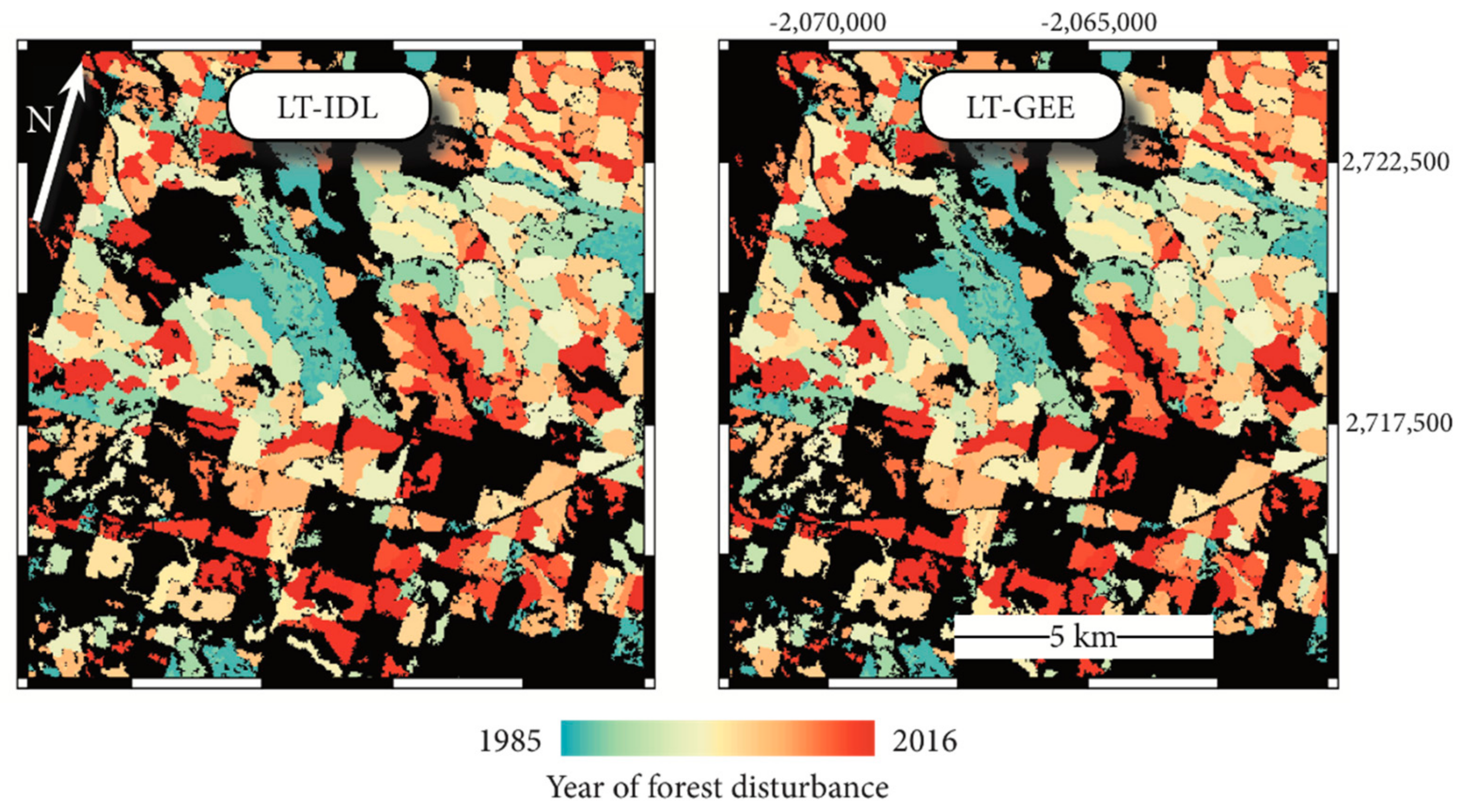
The above comparisons suggest that the LT-GEE algorithm mimics the vertex-identification and fitting of the LT-IDL version, but a simple disturbance mapping exercise may be of more direct interest to the user community. Therefore, for the four regions with substantial forest cover (Regions 1, 2, 4, and 6; Figure 2b), we applied our standard disturbance mapping approaches (described in [18]) to map abrupt forest disturbance in pixels labeled as forest in the 2001 National Land Cover Database (NLCD; [15]). Despite the differences in handling of spikes, the two algorithms agreed on forest/non-disturbance labeling more than 90% of the time (

Table 2. Agreement between algorithms of forest disturbance and no-disturbance calls for all pixels in the four forest-dominated study regions in Figure 1.

		Disturbance	No Disturb.	GEE Total	Agree-ment		Disturbance	No Disturb.	GEE Total	Agree-ment
Disturbance	Region 1	11.0%	4.1%	15.1%	72.6%	Region 2	37.0%	5.2%	42.2%	87.7%
No Disturb.		3.1%	81.8%	84.9%	96.4%		4.6%	53.2%	57.8%	92.1%
IDL Total		14.1%	85.9%				41.6%	58.4%
Agreement		78.3%	95.2%		92.8%		88.9%	91.1%		90.2%
Disturbance	Region 4	6.1%	4.2%	10.3%	59.0%	Region 6	25.5%	3.3%	28.9%	88.4%
No Disturb.		1.7%	88.0%	89.7%	98.1%		2.6%	68.5%	71.1%	96.3%
IDL Total		7.8%	92.2%				28.2%	71.8%
Agreement		77.6%	95.4%		94.0%		90.7%	95.4%		94.0%

). An example forested region confirms the patterns of agreement; disagreements tend to be at the scale of individual pixels (Figure 5). Note that rates of disturbance disagreement were fairly consistent in all four regions: between 2 and 5% of the pixels disagreed, even though overall disturbance rates varied by a factor of six from Region 4 to Region 2. This suggests a randomized spatial process of disagreement that is consistent with the logic error fixes. Where disagreements occurred, they were essentially balanced between the two algorithms, again consistent with an unbiased, essentially random process associated with vagaries of despiking. For pixels where both algorithms agreed that disturbance occurred; they agreed on the year of disturbance more than 97% of the time and had nearly identical magnitudes. For pixels where year of disturbance was different, magnitude discrepancies were largely balanced around zero, again suggesting small random differences. Although the scope of this technical note focuses on evaluating the agreement among the two versions of the algorithm rather than against independent data, we encourage the interested reader to explore two other studies in which the LT-GEE algorithm was evaluated against independent disturbance data [17,19].

5. Conclusions

We translated LandTrendr, a trajectory-based change detection algorithm for time series Landsat imagery, from its original instance in the IDL software language to an operational function in Google Earth Engine (LT-GEE). Some small errors in the original code were found during transliteration and were corrected. Comparisons of the two algorithms confirm that the LT-GEE implementation functions appropriately. Code and documentation for the LT-GEE implementation can be found at https://github.com/eMapR/LT-GEE).