Coastal Improvements for Tide Models: The Impact of ALES Retracker

Abstract

Since the launch of the first altimetry satellites, ocean tide models have been improved dramatically for deep and shallow waters. However, issues are still found for areas of great interest for climate change investigations: the coastal regions. The purpose of this study is to analyze the influence of the ALES coastal retracker on tide modeling in these regions with respect to a standard open ocean retracker. The approach used to compute the tidal constituents is an updated and along-track version of the Empirical Ocean Tide model developed at DGFI-TUM. The major constituents are derived from a least-square harmonic analysis of sea level residuals based on the FES2014 tide model. The results obtained with ALES are compared with the ones estimated with the standard product. A lower fitting error is found for the ALES solution, especially for distances closer than 20 km from the coast. In comparison with in situ data, the root mean squared error computed with ALES can reach an improvement larger than 2 cm at single locations, with an average impact of over 10% for tidal constituents $K_2$, $O_1$, and $P_1$. For $Q_1$, the improvement is over 25%. It was observed that improvements to the root-sum squares are larger for distances closer than 10 km to the coast, independently on the sea state. Finally, the performance of the solutions changes according to the satellite’s flight direction: for tracks approaching land from open ocean root mean square differences larger than 1 cm are found in comparison to tracks going from land to ocean.

1. Introduction

The ability to predict tides in coastal areas is of crucial importance for our society. In certain regions, tidal events combined with extreme meteorological conditions are responsible for severe flooding and consequent environmental issues. Another critical function of tide models is related to ocean satellite altimetry: altimetric measurements need to be corrected for tidal signal in order to separate the tidal-related variability of sea level from the anomalies coming from the ocean dynamic topography. Therefore, more accurate tide models result in more reliable altimetric sea level retrievals. During the last decades, improvements in oceanographic models and observation techniques brought remarkable results in tide monitoring and prediction. A fundamental benefit comes from satellite altimetry, which provides global-scale sea-level observations with an accuracy of few centimeters [1]. These measurements are mainly exploited in modern tide models as constraint for hydrodynamic modeling, or to empirically derive tidal information from satellite sea-level time-series. As described by [2], after the exploitation of satellite data TOPEX/Poseidon (launched in 1992) tide models showed an enhancement of approximately 5 cm over the previous models. However, significant errors for the major constituents $M_2$ and $S_2$ were found at high latitudes [3]. Also, low accuracy was observed in shallow waters, where tidal constituents are highly dependent on bathymetry and the shape of the oceanic shelf [4]. Major efforts in these areas brought a dramatic progress for shallow-water tides, with a consequent larger agreement among different models, and a clear improvement on the single constituents [5]. However, lower performances were observed in coastal regions, resulting in large discrepancies among the models. For models assimilating satellite measurements such situation may be due to a poor availability and quality of altimetric data, highly influenced by the presence of land [6], patches of water at very low sea state within the altimeter footprint [7], or ice [8]. In these areas, the returned echo assumes shapes that are considerably different from the typical open ocean radar return and therefore the signal needs to be fitted with a dedicated algorithm (called retracker). Exploiting these recent advances in data pre-processing, some dedicated coastal products are currently available [9].

The purpose of this paper is to assess the influence of a tailored coastal retracking method on the quality of an ocean tide model, which is an important step towards more oceanographic applications of coastal altimetry [10]. In other words, we want to quantify the difference at the coast between tidal constituents estimated with a dedicated coastal retracker and the same constituents derived with an ordinary open ocean retracker. The coastal retracker used for this experiment is the Adaptive Leading Edge Subwaveform (ALES) retracker. The reliability of this retracker has been proven in a number of applications such as the regional estimation of the seasonal cycle and trend of the sea level [11,12]. Moreover, improvements in areas with a complex macrotidal regimes were validated in [13]. The approach applied to derive the tidal constituents represents a prototype of the new Empirical Ocean Tide (EOT) model. This model takes advantage of the most recent altimetric products, with focus on coastal performances. The model scheme follows the former EOT11a approach [3]: residual tidal constituents are derived on a least-squares-based harmonic analysis applied to Sea Level Anomalies (SLA). In this case, an along-track solution was preferred compared to the classical grids in order to study the evolution of the performances and the impact of the retrackers with respect to the distance to the coast. The data used for the model are illustrated in Section 2 together with a brief description of the ALES retracker and the in situ dataset used for the comparison of the models (Section 2.1 and Section 2.2). A more detailed explanation of the tide model approach can be found in Section 3. In Section 4 the methods used for the model comparison are shown, and in Section 5 the results are presented and discussed. Finally, in Section 6 the conclusions and future work are described.

2. Dataset Description

2.1. Altimeter Dataset

In this study, high-rate observations from Jason-1 and Jason-2 missions were used. The high-rate (20 Hz) data allow a ground spatial resolution of circa 350 m along-track, which was preferred over low-rate (1-Hz) products for this dedicated investigation over coastal areas. The data were extracted from the DGFI-TUM’s Open Altimeter Database (OpenADB: https://openadb.dgfi.tum.de), which contains the original Sensor Geophysical Data Records (SGDR) and derived high-level products. Version SGDR-E is available in OpenADB for Jason-1, while for Jason-2 version SGDR-D was used. For the two missions only data provided during the reference orbit phase are included, obtaining a continuous time-series of 14 years, from January 2002 until February 2016. In order to compute the tidal constants, values of Sea Level Anomalies (SLA) are needed. At each point, SLA are calculated according to [14]:

$$\begin{array}{c}\hfill SLA=H-R-h_{MSS}-h_{geo}\end{array}$$

(1)

where H is the orbital height of the satellite, R is the range, $h_{MSS}$ is the height of the Mean Sea Surface (MSS), and $h_{geo}$ is the sum of the heights of all the geophysical corrections. The MSS and the geophysical corrections applied for both missions are listed in

Table 1. List of corrections used to compute Sea Level Anomalies for this study.

Correction	Model	Reference
Mean Sea Surface	DTU15MSS	Andersen et al. [20]
Inverse barometer	Dynamic Atmospheric Correction (DAC)	Carrère et al. [21]
Wet and Dry troposphere	ECMWF	ECMWF [22]
Ionosphere	NOAA Ionosphere Climatology 2009 (NIC09)	Scharroo and Smith [23]
Ocean and Load tide	FES2014	Carrère et al. [24]
Solid Earth and Pole Tide	IERS Conventions 2003	McCarthy and Petit [25]
ALES Sea State Bias	ALES	Passaro et al. [19,26]
SGDR Sea State Bias	SGDR	AVISO/PODAAC [15]

. SLA values are additionally flagged with the following criteria:

• −2.5 m ≤ SLA ≤ 2.5 m [3]
• SWH < 11 m [15]
• 7 dB < BS < 30 dB [15]
• Distance to coast >3 km

where SWH is the Significant Wave Height and BS is the backscatter coefficient. Note that the backscatter coefficient is commonly defined in literature as ${\sigma }_0$, however in this case BS is used to avoid ambiguities with the unit-weight variance (see Section 4). The tidal correction plays an important role in this investigation. The rationale behind the EOT approach consists of the following steps:

• Application of a pre-existing tide model to correct the SLA
• Estimation of residual periodic components associated with tides in the corrected SLA
• Estimation of a new tide correction to adjust and improve the original FES2014 solution

Details on this procedure are given in Section 3. The pre-existing tide model used to correct SLAs is the Finite Element Solution 2014 (FES2014) and it is characterized by new high-resolution and coastal features, essential basis for a coast-dedicated tide model. According to the range used, two experiments are defined in this study: SGDR and ALES. The first uses the range obtained from the ocean retracker of the standard product. This is based on the MLE4 algorithm which adopts the Brown-Hayne (BH) functional form [16,17]. The BH models the expected reflected radar signal from the ocean surface and is considered to be suboptimal in the coastal zone. The second is based on the ALES retracker which restricts the application of BH to only a portion of the fitted radar echo (selected according to a first estimation of the sea state) in order to guarantee the precision of the measurement also in the open ocean, while avoiding spurious reflections typical of the coastal zone. The SSB correction applied depends on the range used. For both the retracking algorithms, the estimates of SSB are also provided. In particular, the ALES SSB is computed using the same SSB model of the SGDR [18] applied to the 20-Hz estimations of SWH and Wind Speed from ALES. This strategy has already been validated with in situ data in [19].

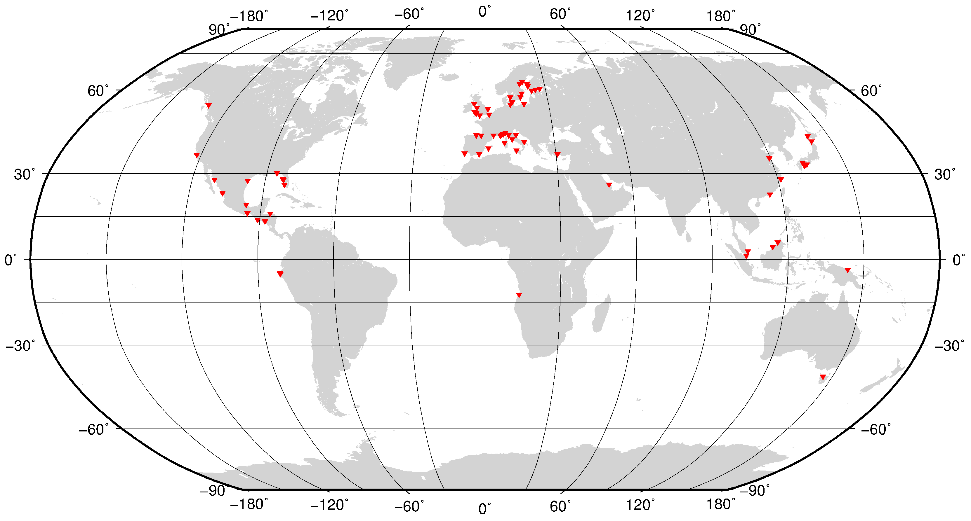
2.2. Tide Gauge Dataset

The harmonic constants resulting from the along-track model are compared against in situ data at the coast. These data were taken from the Global Extreme Sea Level Analysis (GESLA) dataset, which is a unique-format collection of different datasets containing high-frequency (every one hour) sea-level measurements [27]. The harmonic constants used for the comparison were computed via the least-squares method, following e.g., [13]. Within this dataset, tide gauges were selected according to the following criteria:

• Maximum distance to satellite track: 50 km.
• GESLA data already assimilated in FES2014 model (Cancet, personal communication) are discarded.
• Stations near estuaries are discarded. Exceptions for fjords (e.g., Finnish and Canadian coasts).
• Final manual screening on the selected stations: tide gauges with timeseries shorter than one year are discarded while part of the timeseries containing doubtful offsets are not considered.

For each site, one or two crossing tracks were found, obtaining a total of 85 tracks for 70 tide gauges. Their locations are shown in Figure 1.

3. Tide Model Approach

The method used to compute the tidal constants is based on version 11a of DGFI-TUM’s EOT model. For this work, the tidal analysis was based on Jason-1 and Jason-2 missions only, and an along-track solution was chosen. The approach is described in detail hereafter.

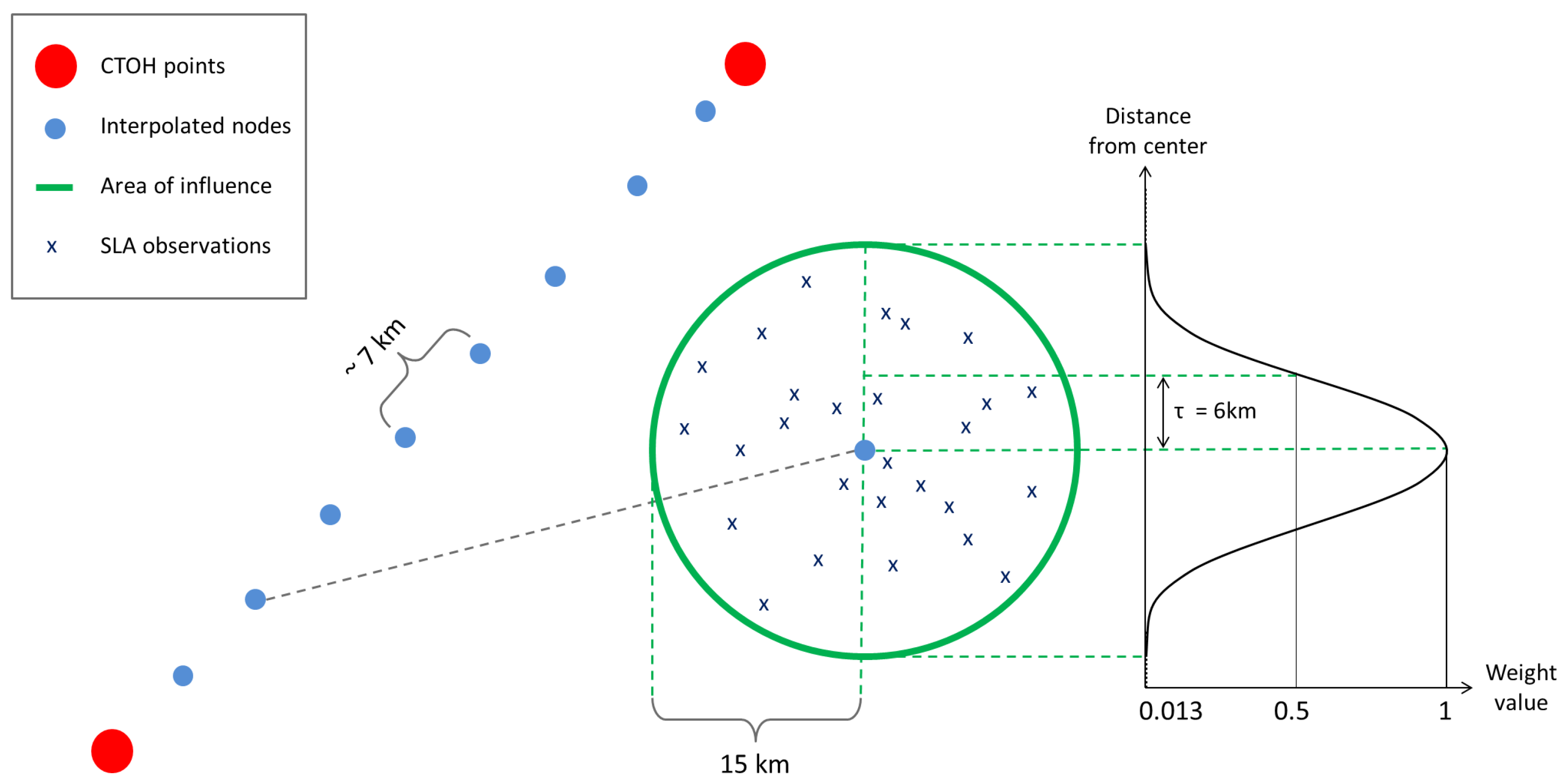
3.1. Selection of the Nodes

In the first step, the tracks of interest were selected according to the position of the tide gauges. The points along track at which the tidal constants were computed (also called nodes) are placed on the reference points belonging to the CTOH Topex/Poseidon nominal path (see acknowledgements), with a distance of circa 7 km between two nodes. Each node represents the center of a circular area of influence with radius (${\psi }_{max}$) 15 km. All the SLA observations located within this area are selected for the tidal analysis. In order to account for the different behavior of SLAs, every observation i is weighted with a Gaussian function inversely proportional to its distance from the node ${\psi }_i$ [3]:

$$\begin{array}{c}\hfill w_i=e^{-\beta {\psi }_i^2}\end{array}$$

(2)

where $w_i$ is the value of the weight, $\psi$ is the distance between the observation and the node, and $\beta$ is defined as:

$$\begin{array}{c}\hfill \beta =\frac{\ln 2}{{\tau }^2}\end{array}$$

(3)

with $\tau =0.4{\psi }_{max}$. The quantity $\tau$ is called half-weight width and determines the steepness of the Gaussian function. Namely, it defines the distance from the node for which the weight has value 0.5; in this case the value of $\tau$ is 6 km. In Figure 2, the node configuration together with the weighting representation is shown.

3.2. Computation of Tidal Constituents

After collecting the SLA observations, the components of the residual tide signal are computed for the main constituents: $M_2$, $N_2$, $S_2$, $K_2$, $K_1$, $O_1$, $P_1$, and $Q_1$. The solution is estimated by a weighted least-squares approach. The unweighted fitting equation for an observation i can be written as [28]:

$$\begin{array}{c}\hfill SL{A}_i=m_j+a·t_i+\sum _{k=1}^n\left(A_k\cos P_k·f_k\cos ({\theta }_k+u_k)+A_k\sin P_k·f_k\sin ({\theta }_k+u_k)\right)\end{array}$$

(4)

Together with the tidal elements, also the j-th mission offset $m_j$ and the slope a—coming from the SLA time series at the node—are calculated [29]. The summation represents the sum of the n tidal constituents which are defined by the amplitude $A_k$, the phase $P_k$, and the given astronomical arguments summarized by the symbol ${\theta }_k$, dependent on the time of the observation $t_i$. The nodal corrections $f_k$ and $u_k$ are also given, and can be obtained according to [30]. $A_k\cos P_k$ and $A_k\sin P_k$ are respectively the unknown coefficients of the in-phase and quadrature components and characterize the residual signal of constituent k. All the known right-hand-side elements of Equation (4) are used to form the design matrix of the least-squares approach. In this study, the weight matrix is diagonal and is filled with the weights of the SLAs computed with Equation (2). In combination with the least-squares estimation, a Variance Component Estimation (VCE) is also applied [3]. The VCE is used to weight the contribution of the different missions following the iterative procedure described in e.g., [31]. Finally, the residuals are added to the FES2014 constituents in order to obtain a full tidal signal, from which the amplitude and phase are derived.

4. Evaluation Methods

The different performances between the derived tide models are compared against the GESLA in situ data by computing the Root-Mean-Square difference (RMS) of their harmonic constants. For a k-th constituent, the RMS is computed as:

$$\begin{array}{c}\hfill RM{S}_k=\sqrt{\frac{{(A_M\cos P_M-A_T\cos P_T)}^2+{(A_M\sin P_M-A_T\sin P_T)}^2}{2}}\end{array}$$

(5)

where $A_M$ and $P_M$ are the amplitude and phase of one solution (SGDR or ALES) for that constituent, and $A_T$ and $P_T$ the ones given by the tide gauge observations. The absolute RMS difference between the SGDR and the ALES solution is written as $\mathsf{\Delta }RM{S}_k=RM{S}_{k,SGDR}-RM{S}_{k,ALES}$ and is measured in cm. The relative RMS difference is also shown, which is described as:

$$\begin{array}{c}\hfill \mathsf{\Delta }RM{S}_k[\%]=\frac{\mathsf{\Delta }RM{S}_k}{RM{S}_{k,SGDR}}·100\end{array}$$

(6)

This difference is expressed in percentage and indicates the relative improvement or worsening of the ALES solution with respect to the SGDR results. For an overall performance, the Root-Sum Squared (RSS) of the available n constituents is also calculated:

$$\begin{array}{c}\hfill RSS=\sqrt{{\displaystyle \sum _{k=1}^n}{RM{S}_k}^2}\end{array}$$

(7)

Both $\mathsf{\Delta }RM{S}_k$ and $RSS$ quantities are estimated for all the nodes along-track. In particular, results for the closest node to the tide gauge of interest (henceforth CNTG) are also considered, as they would represent the accuracies with respect to the coastal true values. To highlight the discrepancies among the ALES and SGDR solutions, it was chosen to express the results in terms of absolute differences, such as:

$$\begin{array}{c}\hfill \mathsf{\Delta }RSS=RS{S}_{SGDR}-RS{S}_{ALES}\end{array}$$

(8)

A positive $\mathsf{\Delta }RSS$ corresponds to higher RSS for the SGDR solutions, and therefore an improvement of ALES solutions with respect to a model using an ordinary retracker. Finally, the internal quality of the models is compared using ${\sigma }_0$, the unit-weight variance of the least-squares fit, and is inversely proportional to the number of observations [32]. The larger is ${\sigma }_0$, the higher is the uncertainty of the fitting.

5. Results and Discussion

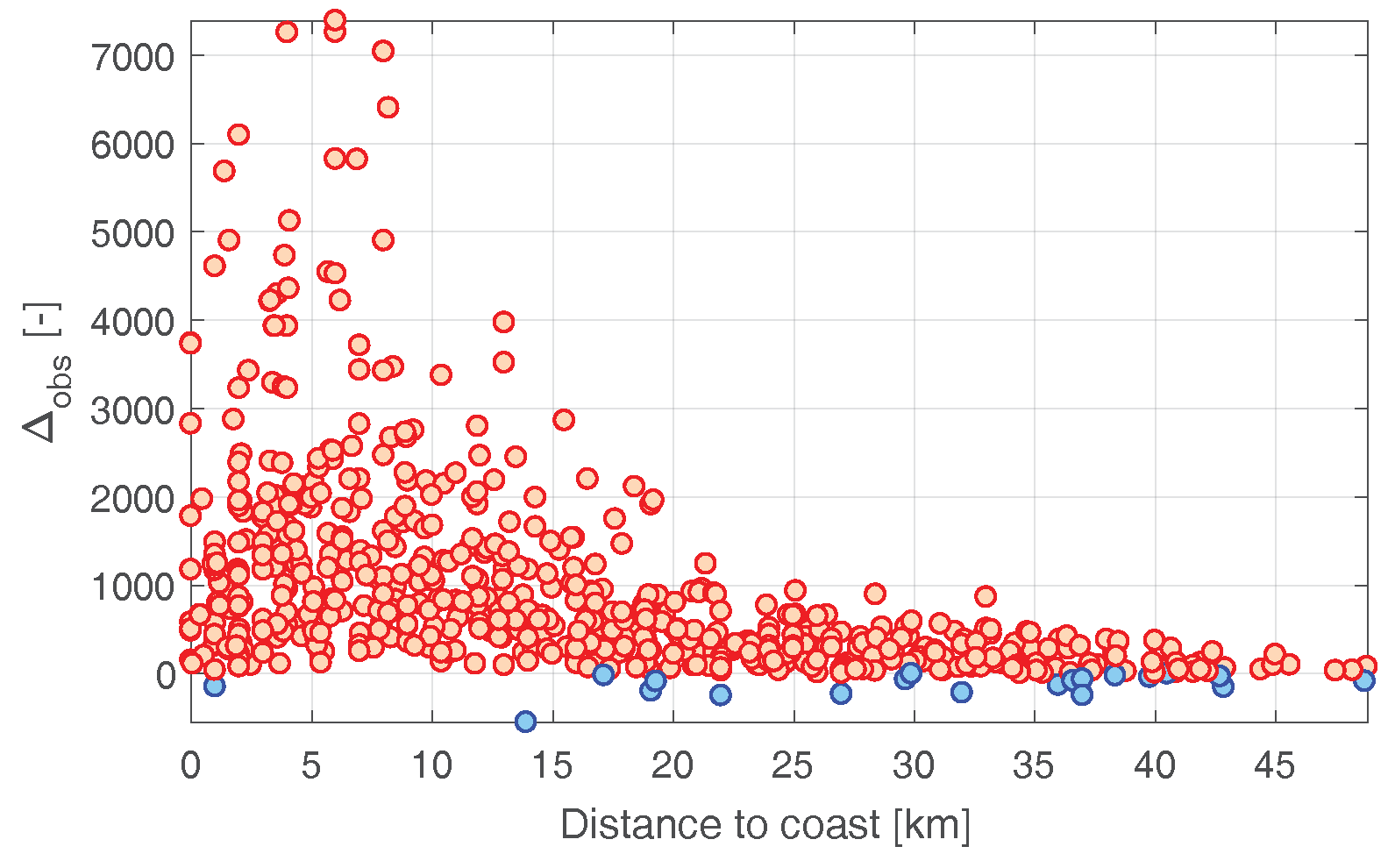
5.1. Number of Observations

One of the most advantageous features of ALES retracker is the large amount of valid coastal measurements available along track. In this work this benefit is shown in terms of observations available for each node. In Figure 3 the difference between the number of observations of ALES and the ones retrieved with SGDR are displayed. This difference is expressed as: ${\mathsf{\Delta }}_{obs}$, i.e., observations of ALES minus observations of SGDR. Each dot represents a node along the tracks, plotted against the distance to the coast. The red markers highlight the positive values, that is, the nodes for which ALES provides a larger amount of data with respect to SGDR. The blue dots are used for the negative values. An interesting, yet expected behavior is observed for values below 20 km from the coast: far more observations are available with ALES while approaching the coast, with some exceptions for few points.

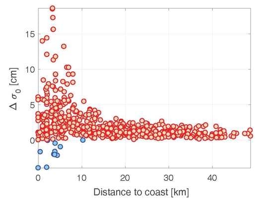
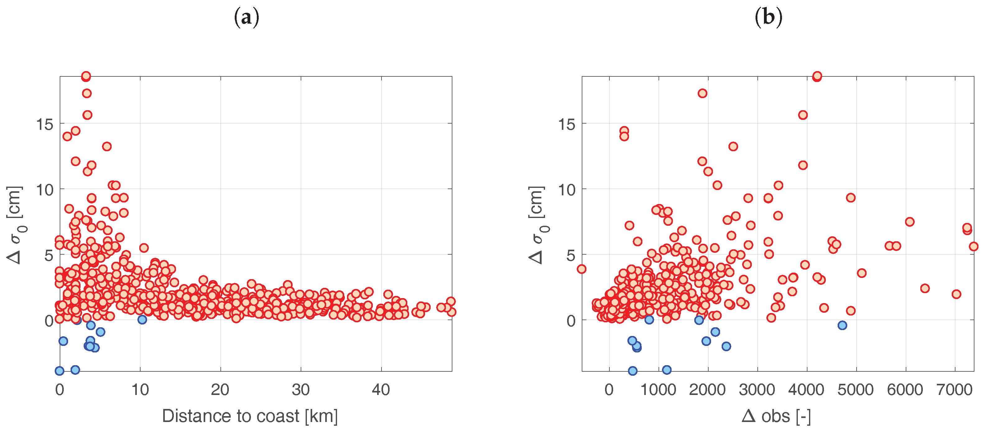
5.2. Fitting Uncertainty

An analogous comparison is shown for the variable ${\sigma }_0$, that represents the quality of the least squares fit. In Figure 4a the difference at each node between the ${\sigma }_0$ computed for the SGDR solutions and ${\sigma }_0$ obtained from ALES is shown. A positive value on the Y the change. -axis (red dots) corresponds to a larger fitting error for the SGDR solutions, and negative values (blue dots) for the contrary. From the plot it is clear that in most cases an improvement for ${\sigma }_0$ is achieved with ALES, with exception for few coastal points. The dependence of ${\sigma }_0$ on the number of observations may explain the smaller errors for ALES. However, from Figure 4b one can notice that large improvements in ${\sigma }_0$ are reached also for a lower amount of data. On the other hand, the few cases with larger internal errors may be found at nodes with more data availability. These special cases, which accounts for only the 1.5% of the cases, may be justified by residual erroneous estimations in the ALES data, which were not identified by the outliers analysis.

5.3. Comparison Against In Situ Data

In this Section the results are compared in terms of RMS and RSS differences against in situ data. The first paragraph gives an overview of the results; the second paragraph discusses the dependency of the results on distance to coast, distance to tide gauge, track direction, and SWH.

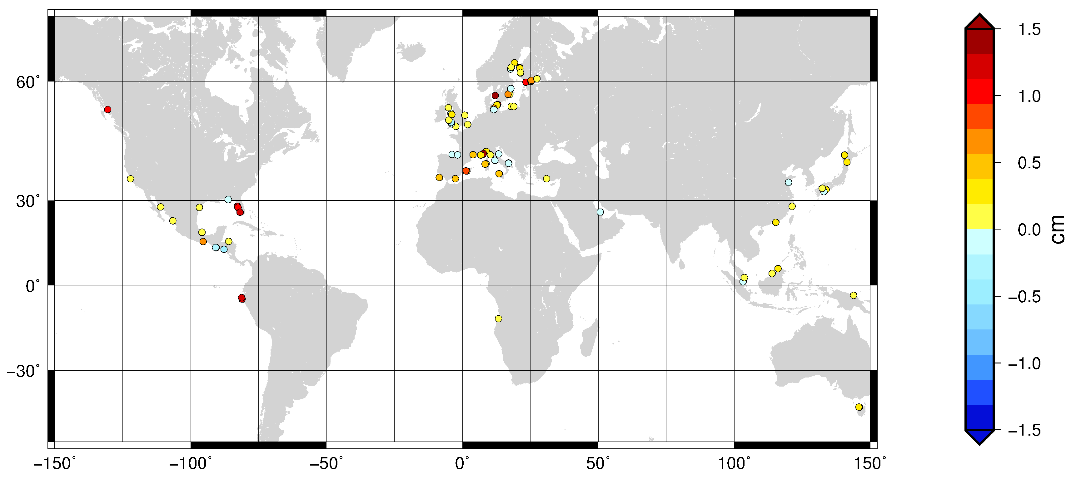
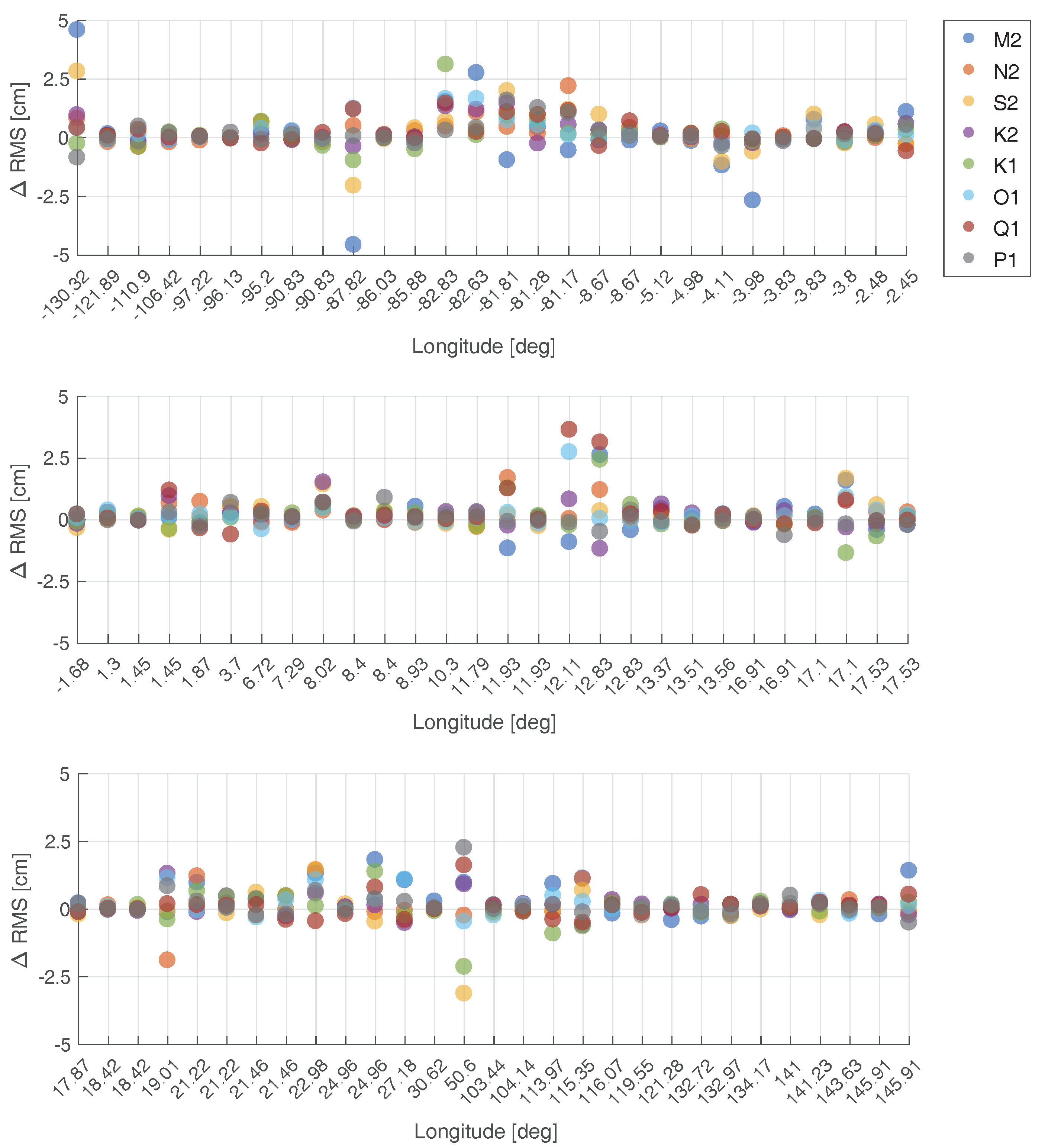
5.3.1. General Results

In Figure 5, the spatial distribution of the absolute differences $\mathsf{\Delta }$RSS are shown. The differences are computed for the CNTG, for all the 85 tracks. In general, improvements are found for 66 tracks, with an average of 0.4 cm and a maximum value of 1.9 cm. The red dots indicate the highest improvements for the ALES solutions, which are located unevenly between Europe and the American continent.These higher values may be due to improvements to only few single constituents. This can be observed in Figure 6, where the absolute $\mathsf{\Delta }$RMS of the closest nodes to the tide gauge of interest are plotted against the longitude of the in situ site. The plot is divided in three rows for an easier visualization, and the $\mathsf{\Delta }$RMS of each tidal constant is color-coded according to the legend. An example of large improvements for single constituents can be seen at Prince Rupert, western Canada, or Ringhals, Sweden (respectively longitudes: −130.32${}^{\circ }$ and 12.11${}^{\circ }$), where the values of $\mathsf{\Delta }$RMS for $M_2$ and $S_2$ for Prince Rupert, or $Q_1$ and $O_1$ are larger than 2.5 cm. In contrast, there are locations such as La Union, El Salvador, and Swansea, UK (longitudes −87.82${}^{\circ }$ and −3.98${}^{\circ }$) where the ALES solution shows a loss in performance—again differences larger than 2.5 cm—for constituent $M_2$. The RMS differences for all the 85 tracks are summarized in

Table 2. Average of RMS for major constituents for the closest points to the tide gauges. The values are expressed in cm. The last column shows the relative difference between the two solutions.

Constituents	${\mathit{RMS}}_{\mathit{ALES}}$ (cm)	${\mathit{RMS}}_{\mathit{SGDR}}$ (cm)	$\mathsf{\Delta }\mathit{RMS}$ (%)
M2	8.0	8.2	2.4
N2	2.1	2.3	8.7
S2	3.5	3.7	5.4
K2	1.4	1.6	12.5
K1	2.1	2.2	4.5
O1	1.4	1.6	12.5
Q1	0.8	1.1	27.3
P1	1.2	1.4	14.3

. The average values were computed using the single RMS values obtained at each site, at the CNTG. A mean improvement of 2 mm can be measured for the ALES solutions with respect to SGDR. It is important to stress that in the global average, results based on ALES are superior to results based on SGDR for every constituent. For K2, O1 and P1 the improvement is over 10%. For Q1, the improvement is over 25%. For larger RMS (such as $M_2$ and $S_2$) a minor effect of ALES is observed for the relative differences.

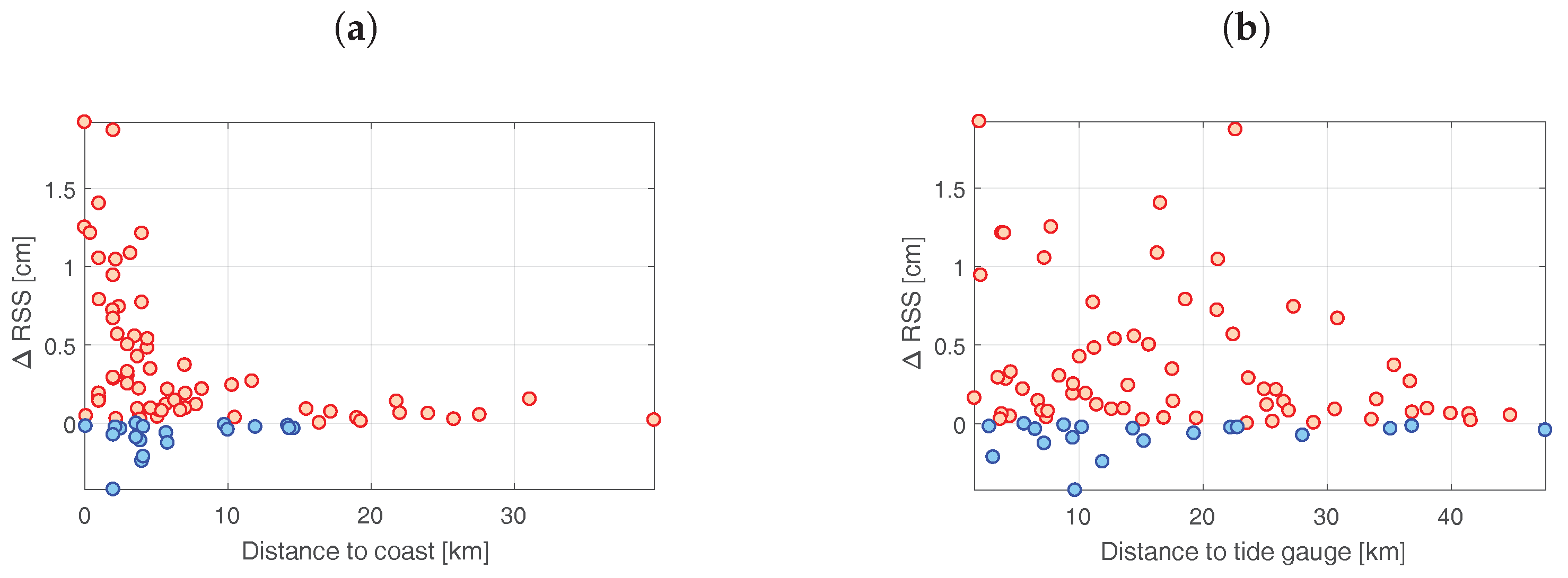
5.3.2. Study of the Dependencies

Also in this section, the CNTGs are used to study the performances of the two retracker solutions. It must be pointed out that the CNTGs may not coincide with the closest points to the coast, as they depend on the position of the track with respect to land. For this reason, it was chosen to analyze the $\mathsf{\Delta }$RSS values against the distance to coast (Figure 7a) as well as against the distance to the tide gauge of interest (Figure 7b). The first plot shows not only that the nodes are mostly concentrated within 10 km to the coast, but also that improvements with ALES larger than 0.5 cm occur for nodes closer than 5 km. On the other hand, no visible dependency is observed between the values of $\mathsf{\Delta }$RSS and their distance from the tide gauge: in fact, the same improvements over 0.5 cm appear also for distances above 20 km. The dependency on the distance to the coast is also shown for the $\mathsf{\Delta }$RMS of the single constituents, Figure 8. Within 10 km from the coast, improvements below 2 cm can be found for all constituents. Larger variability is observed for the major constituents, and single values can reach e.g., $\pm 5$ cm for $M_2$ and $\pm 3$ cm for $S_2$.

Another aspect analyzed is the influence of the track direction on the results, because the performance of a retracker may change whether the satellite approaches land from ocean or flies from ocean to land, as well as if there is a bay (case: land-ocean-land) or the coast is parallel to the track (case: parallel to land). These results are shown in

Table 3. Average of RMS computed for major constituents at the closest points to the tide gauges. The averages are computed after dividing the tracks according to their position with respect to the coast. The values are in cm.

Constituents	Land to Ocean: 30		Ocean to Land: 34		Land-Ocean-Land: 15		Parallel to Land: 6
	$\mathit{R}\mathit{M}{\mathit{S}}_{\mathit{A}\mathit{L}\mathit{E}\mathit{S}}$	$\mathit{R}\mathit{M}{\mathit{S}}_{\mathit{S}\mathit{G}\mathit{D}\mathit{R}}$	$\mathit{R}\mathit{M}{\mathit{S}}_{\mathit{A}\mathit{L}\mathit{E}\mathit{S}}$	$\mathit{R}\mathit{M}{\mathit{S}}_{\mathit{S}\mathit{G}\mathit{D}\mathit{R}}$	$\mathit{R}\mathit{M}{\mathit{S}}_{\mathit{A}\mathit{L}\mathit{E}\mathit{S}}$	$\mathit{R}\mathit{M}{\mathit{S}}_{\mathit{S}\mathit{G}\mathit{D}\mathit{R}}$	$\mathit{R}\mathit{M}{\mathit{S}}_{\mathit{A}\mathit{L}\mathit{E}\mathit{S}}$	$\mathit{R}\mathit{M}{\mathit{S}}_{\mathit{S}\mathit{G}\mathit{D}\mathit{R}}$
M2	6.6	6.9	4.8	5.0	19.3	19.2	4.6	4.7
N2	1.7	1.8	1.3	1.6	4.8	5.2	1.4	1.4
S2	3.1	3.2	2.1	2.4	7.7	7.8	2.6	2.5
K2	1.2	1.3	1.0	1.3	2.8	2.9	1.7	1.7
K1	1.9	1.9	1.4	1.5	3.8	4.2	2.2	2.2
O1	1.2	1.3	1.0	1.3	2.5	2.7	1.6	1.6
Q1	0.8	0.9	0.7	1.0	1.3	1.8	0.9	1.0
P1	1.5	1.7	0.7	0.9	1.9	1.9	1.1	1.2
RSS	8.4	8.5	5.8	6.4	22.1	22.8	6.5	6.6

. The four main headers indicate the track position and the number of tracks used for the RMS average. The RSS computed from the RMS averages for each case are also displayed in the last row of the table. In general, lower values are found for the ALES solution, with exception of few constituents. An interesting result regards the transition land/ocean (i.e., the first four columns): both SGDR and ALES solutions show a higher performance for all constituents for the case ocean-to-land, against the land-to-ocean results, reaching differences larger than 1 cm for single constituents. This can be seen also from the averaged RSS, which show discrepancies of 26 mm between the ALES solutions and 21 mm for SGDR. This situation may be justified by a different behavior of the on-board tracker according to the flight direction, which may consequently influence the performance of the retrackers [7]. A clear example is presented in Figure 9, where the RMS of constituent $M_2$, computed for the ALES solution, is plotted for the nodes of tracks 111 and 92. Track 111 is ascending, and it goes from ocean to land, while track 92 is descending, going from land to ocean. It can be observed, that even though few nodes at track 92 are closer to the tide gauge, they still show a larger RMS with respect to nodes belonging to track 111. Moreover, larger discrepancies are found between ALES and SGDR for the case ocean-to-land, for which RSS values differ of 6 mm against 1 mm in the land-to-ocean case. Unfortunately, for the cases land-ocean-land and parallel-to-land only few tracks were available. However, from both the single RMS and the RSS values similar performance is found between ALES and SGDR solutions.

Finally, the sea state dependency is shown for the absolute $\mathsf{\Delta }$RSS. It was chosen to represent the sea state as the average of the SWH at each node, plus its standard deviation. The SWH values are taken from the ALES product. While the improvement of the ALES data for calm sea states (<2.5 m) is expected [33], the available literature concerning data quality in comparison with SGDR for wavy seas is still scarce. Indeed, from Figure 10, relevant improvements (>0.5 cm) are observed for sea states within 2.5 m, while only few examples are available for high states. However, $\mathsf{\Delta }$RMS > 1 cm are found above 3 m, showing no sensitive relation between the sea state and the data analyzed.

6. Conclusions and Outlook

In this work, we have tested the impact of a coast-dedicated retracker on the estimation of ocean tidal constituents. The experiment aimed to compare tidal constants computed with the standard SGDR product against the ALES coastal retracker. The tidal constituents were derived on nodes defined along Jason satellites’ tracks, applying the method of weighted least-squares on SLA which were previously corrected for the FES2014 tide model. The results were compared with in situ observations in terms of RMS and RSS values. It was shown that with ALES an increased number of sea level retrievals were available at each node, especially at distances closer than 20 km from the coast. The largest improvements are detected at distances within 10 km to the coast, independently from the geographical location and the sea state. A similar behavior was detected for the least-squares fitting error, which also show no clear dependency on the number of observations. In addition, no evident dependency is found for the RMS improvements to the distance to the tide gauges. The general $\mathsf{\Delta }$RSS results over the track nodes showed an average improvement of 0.4 cm for 66 tracks. However, the averaged RMS suggest a mean impact of few mm for all tidal constants. The $\mathsf{\Delta }$RMS highlighted a positive impact of ALES for single constituents, which can reach values >2.5 cm.

The RMS averages were presented after dividing the results according to the satellite’s flight direction. From this experiment it was possible to see that the performance of both solutions change according to the track direction. The transition ocean-to-land shows smaller RMS for both ALES and SGDR solutions, and for all constituents. Single differences may exceed 1 cm when compared with land-to-ocean solutions.

In conclusion, improvements independent from the node position, together with a lower fitting error and a large data availability, make ALES a favorable choice for coastal tidal analysis. Indeed, the retracker will be exploited within the the new version of the EOT model. However, future research should be extended to minor tidal constituents, as well as dedicated regional analyses.

The improvements shown in this study were found despite the ALES retracking strategy was only applied in the residual analysis of the EOT procedure, while the original FES2014 model, which corrects for most of the tidal variability, is still based on SGDR data. We expect therefore that the use of ALES data could bring a decisive improvement in coastal tide modeling if used as a data source to estimate the full tidal component of the sea level variability. Finally, we recommend further investigations aimed to quantify the impact of additional altimetric corrections on the tidal estimation at the coast and to promote more oceanographic applications of coastal altimetry data.

References

1. Bonnefond, P.; Haines, B.J.; Watson, C. In situ absolute calibration and validation. In Coastal Altimetry; Vignudelli, S., Kostianoy, A.G., Cipollini, P., Benveniste, J., Eds.; Springer: Berlin/Heidelberg, Germany, 2011; pp. 259–296. ISBN 978-3-642-12795-3. [Google Scholar]
2. Shum, C.K.; Woodworth, P.L.; Andersen, O.B.; Egbert, G.D.; Francis, O.; King, C.; Klosko, S.M.; Provost, C.L.; Li, X.; Molines, J.-M.; et al. Accuracy assessment of recent ocean tide models. J. Geophys. Res. 1997, 102, 25173–25194. [Google Scholar] [CrossRef]
3. Savcenko, R.; Bosch, W. EOT11a—Empirical Ocean Tide Model From Multi-Mission Satellite Altimetry; DGFI Report No. 89; Deutsches Geodätisches Forschungsinstitut: Munich, Germany, 2012. [Google Scholar] [CrossRef]
4. Andersen, O.B. Shallow water tides in the Northwest European shelf region from TOPEX/POSEIDON altimetry. J. Geophys. Res. 1999, 104, 7729–7741. [Google Scholar] [CrossRef]
5. Stammer, D.; Ray, R.D.; Andersen, O.B.; Arbic, B.K.; Bosch, W.; Carrère, L.; Cheng, Y.; Chinn, D.S.; Dushaw, B.D.; Egbert, G.D.; et al. Accuracy assessment of global barotropic ocean tide models. Rev. Geophys. 2014, 52, 243–282. [Google Scholar] [CrossRef]
6. Gommenginger, C.; Thibaut, P.; Fenoglio-Marc, L.; Quartly, G.; Deng, X.; Gómez-Enri, J.; Challenor, P.; Gao, Y. Retracking altimeter waveforms near the coasts. In Coastal Altimetry; Vignudelli, S., Kostianoy, A.G., Cipollini, P., Benveniste, J., Eds.; Springer: Berlin/Heidelberg, Germany, 2011; pp. 61–101. ISBN 978-3-642-12795-3. [Google Scholar]
7. Passaro, M.; Cipollini, P.; Vignudelli, S.; Quartly, G.D.; Snaith, H.M. ALES: A multi-mission adaptive subwaveform retracker for coastal and open ocean altimetry. Remote Sens. Environ. 2014, 145, 173–189. [Google Scholar] [CrossRef] [Green Version]
8. Andersen, O.B.; Piccioni, G. Recent Arctic sea level variations from satellites. Front. Mar. Sci. 2016, 3, 76. [Google Scholar] [CrossRef] [Green Version]
9. Cipollini, P.; Benveniste, J.; Birol, F.; Fernandes, M.J.; Passaro, M.; Vignudelli, S. Satellite altimetry in coastal regions. In Satellite Altimetry over Oceans and Land Surfaces; Stammer, D., Cazenave, A., Eds.; CRC Press: Boca Raton, FL, USA, 2017; pp. 343–380. [Google Scholar]
10. Liu, Y.; Weisberg, R.H.; Vignudelli, S.; Roblou, L.; Merz, C.R. Comparison of the X-TRACK altimetry estimated currents with moored ADCP and HF radar observations on the West Florida Shelf. Adv. Space Res. 2012, 50, 1085–1098. [Google Scholar] [CrossRef]
11. Passaro, M.; Fenoglio-Marc, L.; Cipollini, P. Validation of Significant Wave Height from improved satellite altimetry in the German Bight. IEEE Trans. Geosci. Remote Sens. 2015, 53, 4. [Google Scholar] [CrossRef]
12. Passaro, M.; Dinardo, S.; Quartly, G.D.; Snaith, H.M.; Benveniste, J.; Cipollini, P.; Lucas, B. Cross-calibrating ALES Envisat and CryoSat-2 Delay-Doppler: A coastal altimetry study in the Indonesian Seas. Adv. Space Res. 2016, 58, 289–303. [Google Scholar] [CrossRef]
13. Lago, L.S.; Saraceno, M.; Ruiz-Etcheverry, L.A.; Passaro, M.; Oreiro, F.A.; D’Onofrio, E.E.; González, R. Improved sea surface height from satellite altimetry in coastal zones: A case study in Southern Patagonia. IEEE J. Sel. Top. Appl. Earth Obs. Remote Sens. 2017, 10, 3493–3503. [Google Scholar] [CrossRef]
14. Andersen, O.B.; Scharroo, R. Range and geophysical corrections in coastal regions—And implications for mean sea surface determination. In Coastal Altimetry; Vignudelli, S., Kostianoy, A.G., Cipollini, P., Benveniste, J., Eds.; Springer: Berlin/Heidelberg, Germany, 2011; pp. 103–145. ISBN 978-3-642-12795-3. [Google Scholar]
15. Picot, N.; Case, K.; Desai, S.; Vincent, P.; Bronner, E. AVISO and PODAAC User Handbook. IGDR and GDR Jason Products; SALP-MU-M5-OP-13184-CN (AVISO), JPL D-21352 (PODAAC); Physical Oceanography Distributed Active Archive Center: Pasadena, CA, USA, 2012. [Google Scholar]
16. Brown, G. The average impulse response of a rough surface and its applications. IEEE Trans. Antennas Propag. 1977, 25, 67–74. [Google Scholar] [CrossRef]
17. Hayne, G.S. Radar altimeter mean return waveforms from near-normal- incidence ocean surface scattering. IEEE Trans. Antennas Propag. 1980, 28, 687–692. [Google Scholar] [CrossRef]
18. Tran, N.; Thibaut, P.; Poisson, J.-C.; Philipps, S.; Bronner, E.; Picot, N. Impact of Jason-2 wind speed calibration on the sea state bias correction. Mar. Geod. 2011, 34, 3–4. [Google Scholar] [CrossRef]
19. Gómez-Enri, J.; Cipollini, P.; Passaro, M.; Vignudelli, S.; Tejedor, B.; Coca, J. Coastal altimetry products in the strait of Gibraltar. IEEE Trans. Geosci. Remote Sens. 2016, 54, 99. [Google Scholar] [CrossRef]
20. Andersen, O.B.; Stenseng, L.; Piccioni, G.; Knudsen, P. The DTU15 MSS (Mean Sea Surface) and DTU15LAT (Lowest Astronomical Tide) reference surface. In Proceedings of the ESA Living Planet Symposium 2016, Prague, Czech Republic, 9–13 May 2016. [Google Scholar]
21. Carrère, L.; Faugère, Y.; Bronner, E.; Benveniste, J. Improving the dynamic atmospheric correction for mean sea level and operational applications of atimetry. In Proceedings of the Ocean Surface Topography Science Team (OSTST) Meeting, San Diego, CA, USA, 19–21 October 2011. [Google Scholar]
22. Persson, A. User Guide to ECMWF Forecast Products; ECMWF: Reading, UK, 2015. [Google Scholar]
23. Scharroo, R.; Smith, W.H.F. A global positioning system-based climatology for the total electron content in the ionosphere. J. Geophys. Res. 2010, 115, 16. [Google Scholar] [CrossRef]
24. Carrère, L.; Lyard, F.; Cancet, M.; Guillot, A.; Picot, N. FES 2014, a new tidal model—Validation results and perspectives for improvements. In Proceedings of the ESA Living Planet Symposium 2016, Prague, Czech Republic, 9–13 May 2016. [Google Scholar]
25. McCarthy, D.D.; Petit, G. (Eds.) IERS Conventions (2003); IERS Technical Note 32; Verlag des Bundesamts für Kartographie und Geodäsie: Frankfurt, Germany, 2004. [Google Scholar]
26. Passaro, M.; Kildegaard Rose, S.; Andersen, O.B.; Boergens, E.; Calafat, F.M.; Dettmering, D.; Benveniste, J. ALES+: Adapting a homogenous ocean retracker for satellite altimetry to sea ice leads, coastal and inland waters. Remote Sens. Environ. 2018, in press. [Google Scholar] [CrossRef]
27. Woodworth, P.L.; Hunter, J.R.; Marcos, M.; Caldwell, P.; Menendez, M.; Haigh, I. Towards a global higher-frequency sea level data set. Geosci. Data J. 2017, 3, 50–59. [Google Scholar] [CrossRef]
28. Savcenko, R.; Bosch, W. Residual tide analysis in shallow water-contribution of ENVISAT and ERS altimetry. In ESA-SP636 (CD-ROM), Proceedings of the Envisat Symposium 2007, Montreux, Switzerland, 23–27 April 2007; Lacoste, H., Ouwehand, L., Eds.; ESA: Noordwijk, The Netherlands, 2007. [Google Scholar]
29. Bosch, W.; Savcenko, R.; Flechtner, F.; Dahle, C.; Mayer-Gürr, T.; Stammer, D.; Taguchi, E.; Ilk, K.H. Residual ocean tide signals from satellite altimetry, GRACE gravity fields, and hydrodynamic modelling. Geophys. J. Int. 2009, 178, 1185–1192. [Google Scholar] [CrossRef]
30. Doodson, A.T.; Warburg, H.D. Admiralty Manual of Tides; H. M. Stationery Off.: London, UK, 1941. [Google Scholar]
31. Teunissen, P.; Amiri-Simkooei, A. Variance component estimation by the method of least-squares. In VI Hotine-Marussi Symposium on Theoretical and Computational Geodesy, Proceedings of the IAG Symposium, Wuhan, China, 29 May–2 June 2006; Xu, P., Liu, J., Dermanis, A., Eds.; Springer: Berlin/Heidelberg, Germany, 2008; ISBN 978-3-540-74583-9. [Google Scholar]
32. Koch, K.-R. Parameter Estimation and Hypothesis Testing in Linear Models, 2nd ed.; Springer: Berlin/Heidelberg, Germany, 1999; ISBN 978-3-540-65257-1. [Google Scholar]
33. Passaro, M.; Cipollini, P.; Benveniste, J. Annual sea level variability of the coastal ocean: The Baltic Sea-North Sea transition zone. J. Geophys. Res. Oceans 2015, 120, 3061–3078. [Google Scholar] [CrossRef]
Figure 1. Location of the in situ data used in this work.
Remotesensing 10 00700 g001
Figure 2. Scheme of the nodes and weighting process. From left to right: the nodes (pale blue) are located over the CTOH track points (red) with a distance of 7 km. For each node a circular area of interest is defined (green), and all the SLA observations (crosses) within this area are selected. The observations are weighted with a Gaussian function dependent on the distance from the node.
Remotesensing 10 00700 g002
Figure 3. Difference in the number of observations between ALES and SGDR at each node against the distance to coast. The blue dots show the cases for which less observations are available for ALES, while the red dots correspond to a larger amount of data for ALES.
Remotesensing 10 00700 g003
Figure 4. Difference of σ 0 values between SGDR minus ALES at each node against the distance to coast (a), and against difference in number of observations between ALES and SGDR (b).
Remotesensing 10 00700 g004
Figure 5. Geographical distribution of the Δ RSS (in cm) for the closest nodes to the tide gauge of interest.
Remotesensing 10 00700 g005
Figure 6. Difference of RMS for major constituents at the CNTG. The values are plotted against the longitude of their location.
Remotesensing 10 00700 g006
Figure 7. Difference of RSS against distance to coast (a) and tide gauge (b) in km. The values are shown for the closest nodes to the tide gauge of interest.
Remotesensing 10 00700 g007
Figure 8. Absolute Δ RMS of major constituents at the CNTG. The values are plotted against the distance to the coast (in km).
Remotesensing 10 00700 g008
Figure 9. RMS values for M 2 constituent computed with ALES solutions for tracks 111 (ascending) and 92 (descending). The tracks face the tide gauge station of Helsinki (diamond-shape marker). The nodes of each track are represented by the round markers and the color shows the value of the RMS with respect to the tide gauge, in cm.
Remotesensing 10 00700 g009
Figure 10. Δ RSS absolute values for the closest node to the tide gauge against the sea state, represented as the averaged SWH computed at each node plus its standard deviation.
Remotesensing 10 00700 g010