Meteo-Marine Parameters from Sentinel-1 SAR Imagery: Towards Near Real-Time Services for the Baltic Sea

1
Department of Marine Systems at Tallinn University of Technology, Tallinn 12618, Estonia
2
German Aerospace Center (DLR), Remote Sensing Technology Institute, Bremen 28199, Germany
*
Author to whom correspondence should be addressed.
Remote Sens. 2018, 10(5), 757; https://doi.org/10.3390/rs10050757
Submission received: 18 April 2018
/
Revised: 8 May 2018
/
Accepted: 9 May 2018
/
Published: 15 May 2018
(This article belongs to the Special Issue Sea Surface Roughness Observed by High Resolution Radar)
Abstract
:A method for estimating meteo-marine parameters from satellite Synthetic Aperture Radar (SAR) data, intended for near-real-time (NRT) service over the Baltic Sea, is presented and validated. Total significant wave height data are retrieved with an empirical function CWAVE_S1-IW, which combines spectral analysis of Sentinel-1A/B Interferometric Wide swath (IW) subscenes with wind data derived with common C-Band Geophysical Model Functions (GMFs). In total, 15 Sentinel-1A/B scenes (116 acquisitions) over the Baltic Sea were processed for comparison with off-shore sea state measurements (52 collocations) and coastal wind measurements (357 colocations). Sentinel-1 wave height was spatially compared with WAM wave model results (Copernicus Marine Environment Monitoring Service (CMEMS). The comparison of SAR-derived wave heights shows good agreement with measured wave heights correlation r of 0.88 and with WAM model (r = 0.85). The wind speed estimated from SAR images yields good agreement with in situ data (r = 0.91). The study demonstrates that the wave retrievals from Sentinel-1 IW data provide valuable information for operational and statistical monitoring of wave conditions in the Baltic Sea. The data is valuable for model validation and interpretation in regions where, and during periods when, in situ measurements are missing. The Sentinel-1 A/B wave retrievals provide more detailed information about spatial variability of the wave field in the coastal zone compared to in situ measurements, altimetry wave products and model forecast. Thus, SAR data enables estimation of storm locations and areal coverage. Methods shown in the study are implemented in NRT service in German Aerospace Center’s (DLR) ground station Neustrelitz.

1. Introduction
1.1. Meteo-Marine Parameters in the Baltic Sea in Relation to Synthetic Aperture Radar
Space-borne Synthetic Aperture Radar (SAR), known for its independence of daylight and weather, can provide two-dimensional (2D) information about the ocean surface with global coverage [1,2]. It is due to the Bragg scattering of the short capillary waves in the dimension of centimeters, produced by wind stress, which allows extraction of wave and wind parameters from radar imagery [3,4,5].
The investigation of SAR ocean surface imaging mechanisms and the extraction of wave and wind parameters started with the launch of L-band SAR onboard SEASAT in 1978 [3,4]. Since then, numerous different algorithms have been developed over time to estimate oceanographic parameters and ocean wave spectra from SAR imagery [6,7,8].
The methods for sea state estimation are largely divided into two main groups; first one being functions where image spectra are transferred into wave spectra using transfer functions (e.g., [6,7,9,10]). These methods are suitable for estimations of swell’s spectra, and its output can be assimilated into spectral wave models. The key to success is to understand the nonlinear SAR imaging of the moving sea surface waves that can be incorporated in “transfer functions” [9]. This approach requires SAR acquisitions with clearly visible wave patterns (e.g., Sentinel-1 Wave Mode (WM) data, high resolution Stripmap Mode TerraSAR-X data). Otherwise, the waves are substantially distorted and are not visible in the SAR images and thus are not represented in the image spectra.
The second group of sea state estimation algorithms use a direct estimation of the wave parameters from the image spectrum with empirical functions (e.g., [11,12,13,14]). Although empirical methods for C-band SAR exist, e.g., CWAVE_ERS and CWAVE_ENVI [12,14], they are only applicable to ERS-2 and Envisat-ASAR WM data. The most recent method for Sentinel-1 WM data by Stopa et al. [15] uses neural network techniques to retrieve wave parameters. However, since Sentinel-1A/B WM data is not available over the coastal areas of world ocean (including the Baltic Sea), moderate resolution Interferometric Wide (IW) swath mode images are used for sea state parameter retrieval. Short windsea waves produce unclear wave pattern in Sentinel-1 IW mode and are hardly distinguishable from ocean clutter. The SAR images are being affected by strong non-linear distortions due to the defocusing effects. Empirical functions, deduced from large sets of representative data, are proven to be more suitable for the short windsea waves and noisy images. The direct estimation of wave parameters from subscene spectra allows fast, straightforward, and reliable near-real-time (NRT) processing of satellite scene while excluding only a fragment of the data [13,16].
For the semi-enclosed micro-tidal Baltic Sea with the absence of long swell waves and short wave “memory” [17], and the significant wave heights remaining mostly between 0 and 2 m (rarely exceeds 4 m [18,19]), the second type of mentioned methods is recommended [13,20,21]. Windsea waves are short-crested and represent a considerable number of small, nonstable, fast, and erratically moving targets for a SAR sensor. Such sea state is typically imaged similar to noise with radar echoes of every scatterer blurred in azimuth and shifted randomly in range direction due to the individual Doppler contribution. The resulting pattern is hardly recognized as a wave pattern. A strong windsea contribution to the total wave height is therefore equivalent to more substantial uncertainties in SAR imaging.
With the launch of C-band Sentinel-1A/B constellation, different methods to estimate meteo-marine parameters, software realizations, and infrastructure open possibilities for NRT services for oceanographic applications [16]. As shortly as 10 min after image downlink, information about wave height, wind speed, as well as ice coverage, oil spills, and ship detection can be transferred to interested institutions or weather services [13,20,22,23,24].
Sentinel-1A/B data is already used worldwide for different applications. For example, estimating wave-induced orbital velocities from which elevation spectra is derived over ice-covered regions [25], calculating significant wave height and mean wave period from Sentinel-1A/B StripMap images using semi-empirical methods [26], or using neural network techniques on Sentinel-1 data to retrieve wave height [15].
SAR-based wave products have also proven to be valuable in the open ocean applications for swell tracking (e.g., [27,28]). In operational wave monitoring and forecasting, several organizations provide relevant information on wave conditions in the Baltic Sea: Baltic Operational Oceanographic System (BOOS), Copernicus Marine Environment Monitoring Service (CMEMS). However, the inclusion of Sentinel-1 wave products over the Baltic Sea into the CMEMS product portfolio would improve the service quality which currently provides only model wave forecast, altimetry wave products, and in situ data [29,30,31].
1.2. Sentinel-1A/B Data over the Baltic Sea
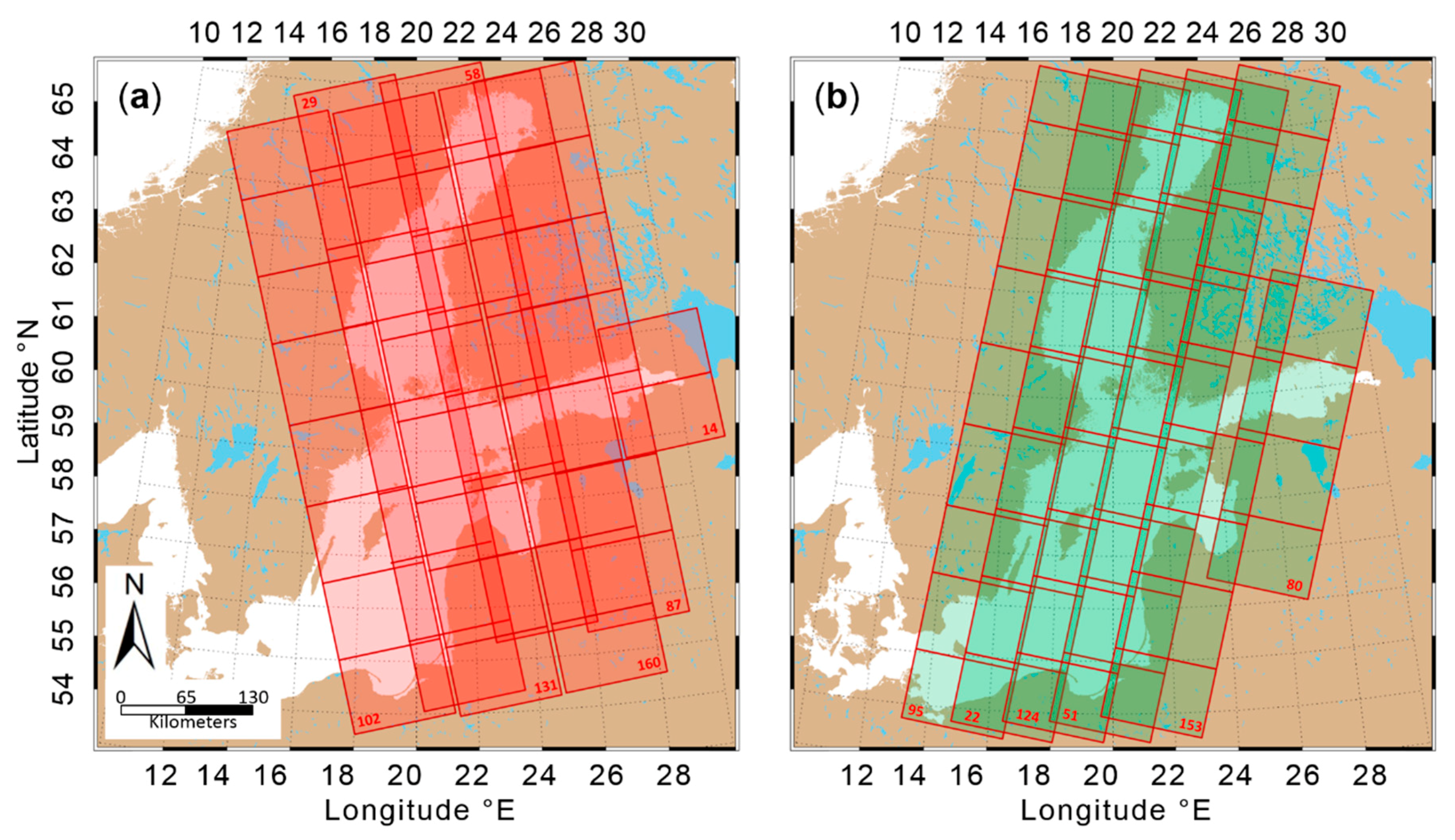
The Baltic Sea is situated in temperate latitudes between 53°N to 66°N and from 9°E to 30°E which makes it one of the most frequently imaged locations by the Sentinel-1 satellites. Various parts of the Baltic Sea are imaged by Sentinel-1A/B daily and often even twice a day by ascending and descending orbits in the morning and in the evening correspondingly. The most suitable Sentinel-1A/B relative orbit numbers are 22 paired with 29, 51 with 58, and 124 with 131 (Figure 1).
Similar usability of satellite SAR data in the Baltic Sea was available when Envisat/ASAR (Advanced Synthetic Aperture Radar) was operational. With the launch of Sentinel-1A/B constellation and the freely available data on the Copernicus Open Access Hub, all the services can be continued. Different methods can be applied on the images to estimate meteo-marine parameters in the Baltic Sea for operational maritime awareness applications. The Sentinel-1 IW level-1 products have 250 km wide swath with 10 m pixel resolution to cover the length of the Baltic Sea with sequential SAR acquisitions.
1.3. Aim of the Study
The main purpose of this study is to assess current state-of-the-art method in estimating meteo-marine parameters, such as wind speed or total significant wave height, in the Baltic Sea from medium resolution Sentinel-1A/B IW swath mode satellite radar imagery. The main advantages of the method as well as challenges are also brought out. The study focuses on the possibilities of making the method available as a near-real-time service over the Baltic Sea using three examples of different sea state in comparison to spectral wave model and available in situ measurements.
The specific objectives of the study are: (i) to validate CWAVE_S1-IW wave retrievals in the Baltic Sea; (ii) to validate CMOD wind speed retrievals in the coastal zone of the Baltic Sea; (iii) to demonstrate potential of Sentinel-1A/B SAR wave retrievals with CWAVE_S1-IW algorithm for operational monitoring in coastal area.
2. Data
2.1. In Situ Data
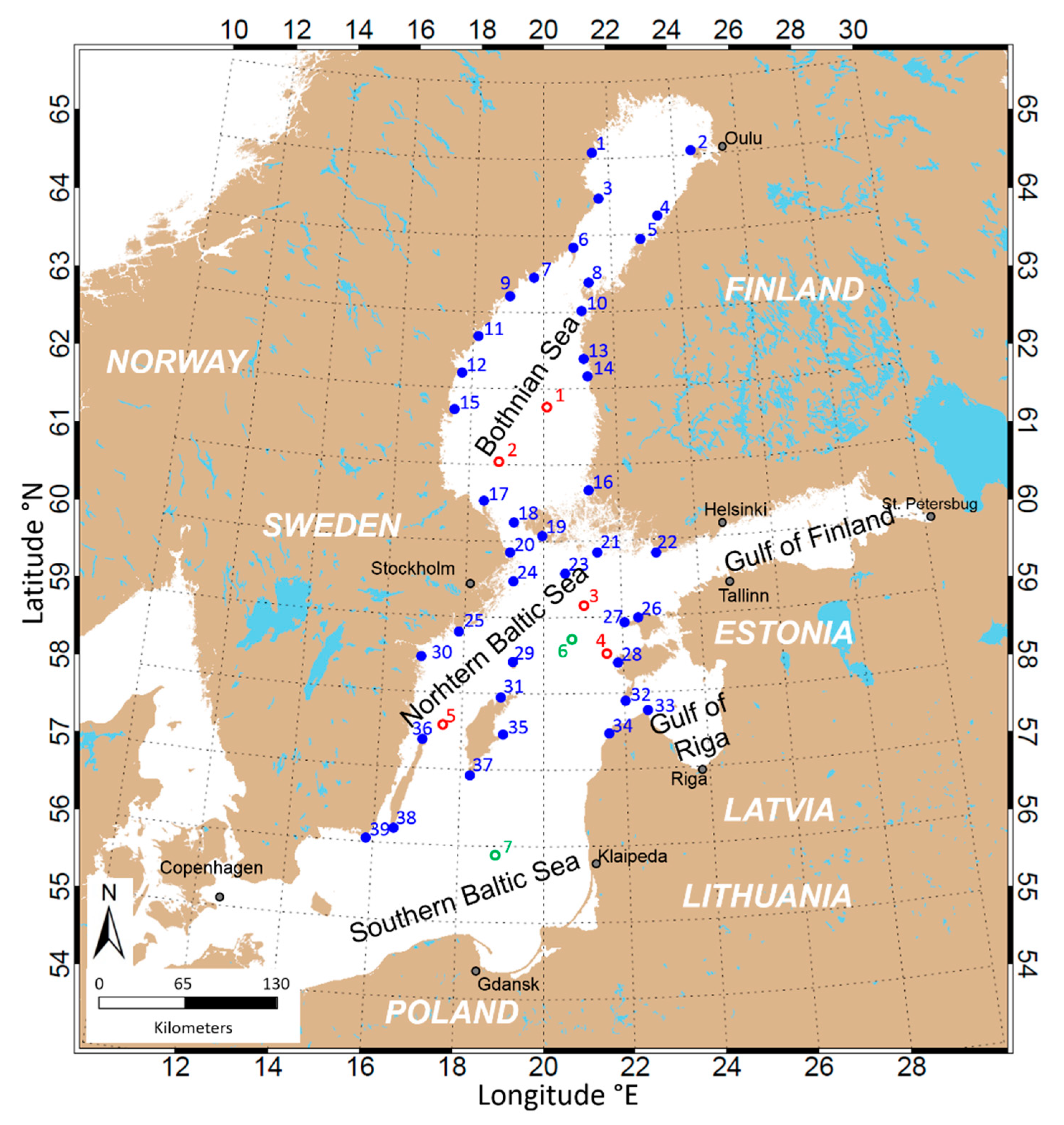
Wind measurement data from 39 coastal stations (357 collocations with SAR data) around the Baltic Sea were used for statistical validation of Sentinel-1 wind retrievals (Figure 2). Sentinel-1 SAR sea state retrievals were validated with in situ wave measurements from 5 offshore stations (52 collocations with SAR data) (Table 1 and Figure 2).
2.2. Sentinel-1A/B Data
The C-band SAR data from Sentinel-1A/B, namely IW mode data, are used for estimation of meteo-marine parameters in this study. The IW mode allows combining large swath width of 250 km in range direction with moderate geometric (5 × 20 m) resolution. Sentinel-1A/B products are available in single (HH or VV) or dual polarizations (HH+HV, VV+VH). For the meteo-marine parameter estimation, either one of the single polarization data is used. The Normalized Radar Cross Section (NRCS) is firstly processed from image pixel digital number (DN):
where is the calibration factor given in the products metadata. The process of estimating sea state parameters is based on FFT (Fast Fourier Transform) of the subscene. Before the analysis, each pixel value of the subscene is normalized resulting in a value :
where is the mean value of in the subscene.
Images were processed with a 3 nautical mile grid with the FFT window of 1024 × 1024 pixels with four-factor resampling and Gaussian smoothing. The processing was implemented for latitudes up to 65°N.
Although all the Sentinel-1A/B IW scenes (460 scenes) over the Baltic Sea from the beginning of 2015 until the end of 2016 were processed, only 15 overpasses (number of acquisitions per satellite overpass ranged from 5 to 9) were selected for validation of the meteo-marine parameter retrieval method as well as for analysis and comparison. All the selected data in Table 2 were acquired in VV polarization. The SAR data for validation were selected to have equal representation of different meteo-marine conditions (i.e., high and low sea states) (Table 2).
2.3. Spectral Wave Model
The wave model WAM [32] is a third-generation wave model which solves the action balance equation without any a priori restriction to the evolution of spectrum. The action density spectrum N is considered instead of the energy density spectrum E because in the presence of ambient currents, action density is conserved, but energy density is not. Action density is related to energy density through the relative frequency [33]:
The variable σ is the relative frequency (as observed in a frame of reference moving with the current velocity) and θ is the wave direction (the direction normal to the wave crest of each spectral component). The action balance equation in Cartesian coordinates reads:
On the left-hand side of Equation (4) the first term represents the local rate of change of action density in time; the second term denotes the propagation of wave energy in two-dimensional geographical space, where is the group velocity and is the ambient current. The third term represents shifting of the relative frequency due to variations in depths and currents (with propagation velocity in space). The fourth term represents depth-induced and current-induced refraction (with propagation velocity in θ space). At the right-hand side of the action balance equation is the source term that represents physical processes which generate, redistribute, or dissipate wave energy in the WAM model. These terms denote, respectively, wave growth by the wind , non-linear transfer of wave energy through four-wave interactions and wave dissipation due to whitecapping and bottom friction .
A pre-operational version of the WAM model which is since April 2017 used for the production of CMEMS wave forecast over the Baltic Sea was used [29]. The model domain covers the Baltic Sea with a grid resolution of one nautical mile, yielding 800 × 775 model grid points. The model was forced with High Resolution Limited Area Model (HIRLAM) winds with a spatial resolution of 11 km and temporal resolution of one hour. In winter, ice concentration data from the Finnish Meteorological Institute’s Ice Service was used. Model grid points in which the ice concentration exceeds 30% are excluded from the calculation. Data assimilation was not used in the wave model.
3. Methods
3.1. Wind
Sea state is strongly dependent on local wind characteristics which SAR data can provide. By analyzing the roughness of the sea, wind speed is received using Geophysical Model Functions (GMF) which relate the local wind conditions and sensor geometry to radar cross section values.
For Sentinel-1 IW data, separate GMFs are used for HH or VV polarizations. For HH, CMOD4 function, developed by Stoffelen et al. [34] is used, and for VV polarization CMOD5.N algorithms shows the best results [35]. The selection of the respective GMF is based on an extensive comparison of GMF performance in comparison with an advanced scatterometer (ASCAT), METOP-A, and METOP-B satellite data performed by [36]. As stated in [36], Thompson polarization ratio [37] with α = 1 is applied to HH polarized data. Also following the authors’ suggestion, a bias of 0.004 is subtracted from VV polarized data, to achieve an overall better agreement with scatterometer data. In total, an accuracy of approximately 1.5 m s−1 has been found in the comparison with the ASCAT data within the validity range of 2–25 m s−1 of the two GMFs [36]. In the current processing procedure, no information from the cross-polar channel is exploited, although a future application of a respective GMF as e.g., proposed by [38] is foreseen to improve wind data reliability in storm situations. The data analyzed in this paper is entirely in the validity range of the applied GMFs for co-polar channels.
In the common procedure, GMFs in general and thus also the CMOD algorithms are inversion methods and require the local wind direction to reduce the number of free parameters in the forward calculation. For the work presented in this paper, wind direction from Weather Research and Forecasting Model (WRF) is used [39]. The model is run for the given area and time of the data acquisition. Initial and boundary conditions are adopted from the corresponding National Oceanic and Atmospheric Administration Global Forecast System (NOAA GFS) analysis model values. For NRT applications, NOAA GFS Forecast values are used instead and the model is run shortly prior to satellite data downlink with a configuration based on the scene parameters (region and time) available in the data processing system schedule. Finally, WRF model values for the wind direction are interpolated to the sea state calculation grid and wind speeds are calculated directly within the sea state algorithm procedure for a given subcell.
3.2. Sea State
An empirical algorithm CWAVE_S1-IW, developed by Pleskachevsky et al. [20], is used to estimate integrated sea state parameters straight from SAR image spectra without transformation into wave spectra. The method is chosen since traditional functions (image spectrum transfer to wave spectrum) are not able to calculate total significant wave height from Sentinel-1 IW mode imagery in the Baltic Sea. The main reasons are the relatively coarse resolution of Sentinel-1A/B and generally lower sea state without long swell compared to the open ocean.
In comparison to e.g., TerraSAR-X/TanDEM-X StripMap scenes with about 3 m resolution, the Sentinel-1A/B IW mode resolution is by an order of magnitude larger. In case of such Sentinel-1 SAR imaging setting the wave structures, if visible, are disturbed by the vast amount of noise. In addition, a standard FFT window of 1024 × 1024 pixels covers a relatively large area of 10240 × 10240 m. To overcome the limitation, four-factor resampling and Gaussian smoothing were applied to selected subscenes. The modified resolution becomes to 2.5 m with areal coverage of 2560 × 2560 m [20].
An important part of sea state estimation is pre-filtering of any natural or man-made objects from subscene which yields to inaccuracies in wave height estimation. Such spectral perturbations result in an integrated value which leads to the total image energy not connected to the sea state. The radar signal disturbances can be divided into two main groups:
- -
- radar signal much stronger than background backscatter from sea state produced mainly by ships or offshore constructions. In these cases, the subscene is additionally analyzed with 100 × 100 m sliding window. The statistics of each window is compared with of the subscene. In a case of with tuned qship value of 2.3 (for 100 × 100 m window), the outliers in the current window are replaced with the mean value of the subscene [20];
- -
- radar signal much weaker than background backscatter from sea state produced, for example, by oil spills, or commonly occurring algae blooms in the Baltic Sea [20]. In those cases, the filtering algorithm was extended by employing with tuned threshold coefficient qspills.
To obtain integrated wave parameters, FFT operation is applied to the radiometrically calibrated subscene. Image power Spectrum is calculated by integration over 2D wavenumber domain:
The integration over wavenumber domain is limited by kmax = 0.003 and kmin = 0.201 which correspond to wavelength of 2000 to 30 m, where wavenumber . In the Sentinel-1A/B image spectra the wavenumber domain ~0.201 < k < 0.060 represents the clutter produced by waves shorter than about 100 m. The domain ~0.060 < k < 0.010 represents long waves with wavelength of ~100 < Lp < 600 m, and the domain ~0.010 < k < 0.003 represents the longest structures such as wind streaks [20].
During the algorithm’s development, it became clear that estimating sea state parameters based only on image spectral properties is not accurate enough. Additional information about each subscene is therefore acquired by using Grey Level Co-occurrence Matrix (GLCM) [40]. By using image texture analysis, accuracy in low and high sea state was improved [20].
The resulting function CWAVE_S1-IW for Sentinel-1A/B imagery to calculate total significant wave height is expressed as:
where is local incidence angle, are coefficients, and are functions of spectral parameters, wind and GLCM results.
The first term in Equation (6) connects the sea state and image spectra energy which contributes the most in the case of long prominent waves with over 100 m wavelengths. The non-linearity of the imaging mechanism is represented by the , which represents noise scaling of total image spectrum energy . The relation , where K serves as a constant found by collocating buoy data, connects the spectrum energy between the wavelength domain of 30–100 m (noisy part of the image spectrum) with the wavelength domain of 100–600 m (the area where wave-looking patterns can be observed). The rest of the terms in Equation (6) represent a series of corrections and filtering of different origins. For example, to consider the wind speed, the term , where , is used. Full information about the function development, tuning and results can be found in [20].
3.3. Comparison Methods
The total significant wave height HS and wind speed U10 derived from SAR are used for comparisons with collocated in situ measurements. The Sentinel-1A/B scenes were processed with 3 × 3 nautical miles posting with ~30 × 45 = ~1350 subscenes per IW image. The collocations were done for five Sentinel-1A/B scenes with a time window of ±20 min and almost 30 min for one case. For the rest of the nine cases, the time difference between the measurements or WAM model data and SAR-derived values is less than 5 min (Table 2). For the spatial collocation, the closest SAR-subscenes are used with a mean value between subscene centre and measurement equipment location or WAM wave model grid point being 4.1 km and 0.7 km, correspondingly. In case the buoy location remains outside the image, the results from the closest subscene to the SAR acquisition edge in the range of up to 10 km was incorporated.
In the case of the wind speed comparison, the average distance between in situ measurement location and the closest subscene centre is 7.7 km. The reason is that the majority of the stations are at the coast (Figure 2) and the SAR subscenes which are close to the shore (contaminated by land backscatter) are filtered out. The time difference remains the same as for wave height comparison, mostly below 5 min.
The Root Mean Square Error (RMSE), Pearson correlation coefficient r, and Scatter Index (SI) (where SI = RMSE/(average of observations)) are calculated for each collocated dataset for the statistical comparisons. Standard deviation (STD) is used to measure variabilities of datasets. All collocated data are presented in scatterplots for wave height and wind speed.
4. Results
4.1. Validation
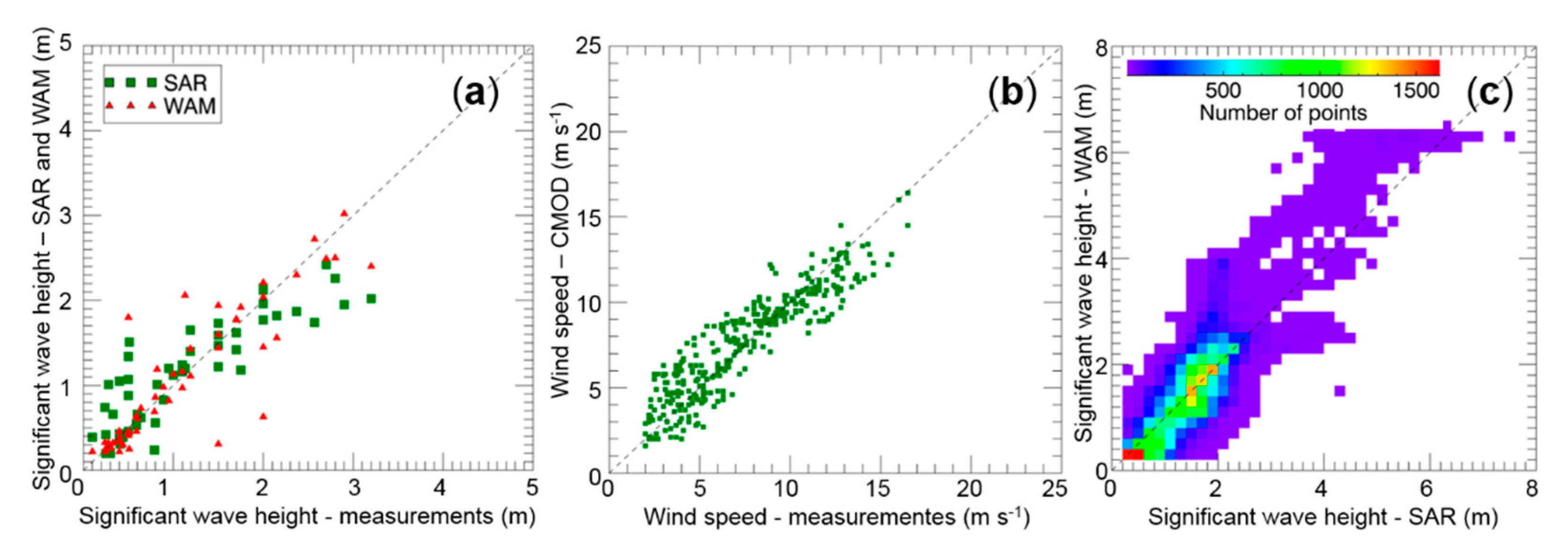
The inter-comparison and the scatter plots in Figure 3 show a good general agreement of SAR wave retrievals and WAM model fields with in situ wave measurements. The corresponding correlation coefficients are 0.88 to 0.89 (Table 3). Also, the RMSE of SAR-derived wave heights and WAM model wave heights are very similar, 0.40 m and 0.39 m correspondingly (Table 3). Slightly poorer statistics (r = 0.81 and RMSE = 0.47 m) are observed when the SAR wave is compared with WAM model data (based on 52 collocated observations), which indicates that SAR and model data resolve distinct aspects of the observed wave parameters. Therefore, SAR and model data could both provide complementary information for accurate description of the wave field. The benefits of multiple data sources for understanding wave field variations are discussed in Section 4.2 and Section 5.1 based on characteristic examples of wave conditions.
Scatter plot on Figure 3b shows the collocated in situ data comparison with estimated wind speed results from the corresponding CMOD algorithm. The wind speed varied from 2 m s−1 to 17 m s−1 with the mean wind speed value of all 357 collocations being 7.53 m s−1. The correlation coefficient between SAR wind retrievals and coastal wind speed measurements was 0.91 (Table 3).
Figure 3c shows the wave height histogram plot of all 49314 SAR-derived values and the corresponding WAM results. Figure 3c clearly indicates that most values are around 1 m. The statistics between the two methods in the case of a larger dataset (49,314 collocations) is slightly better compared to the dataset that was collocated with 52 observations—r = 0.86 and RMSE = 0.47 m (Table 3).
4.2. Case Studies: High, Medium, and Low Sea State
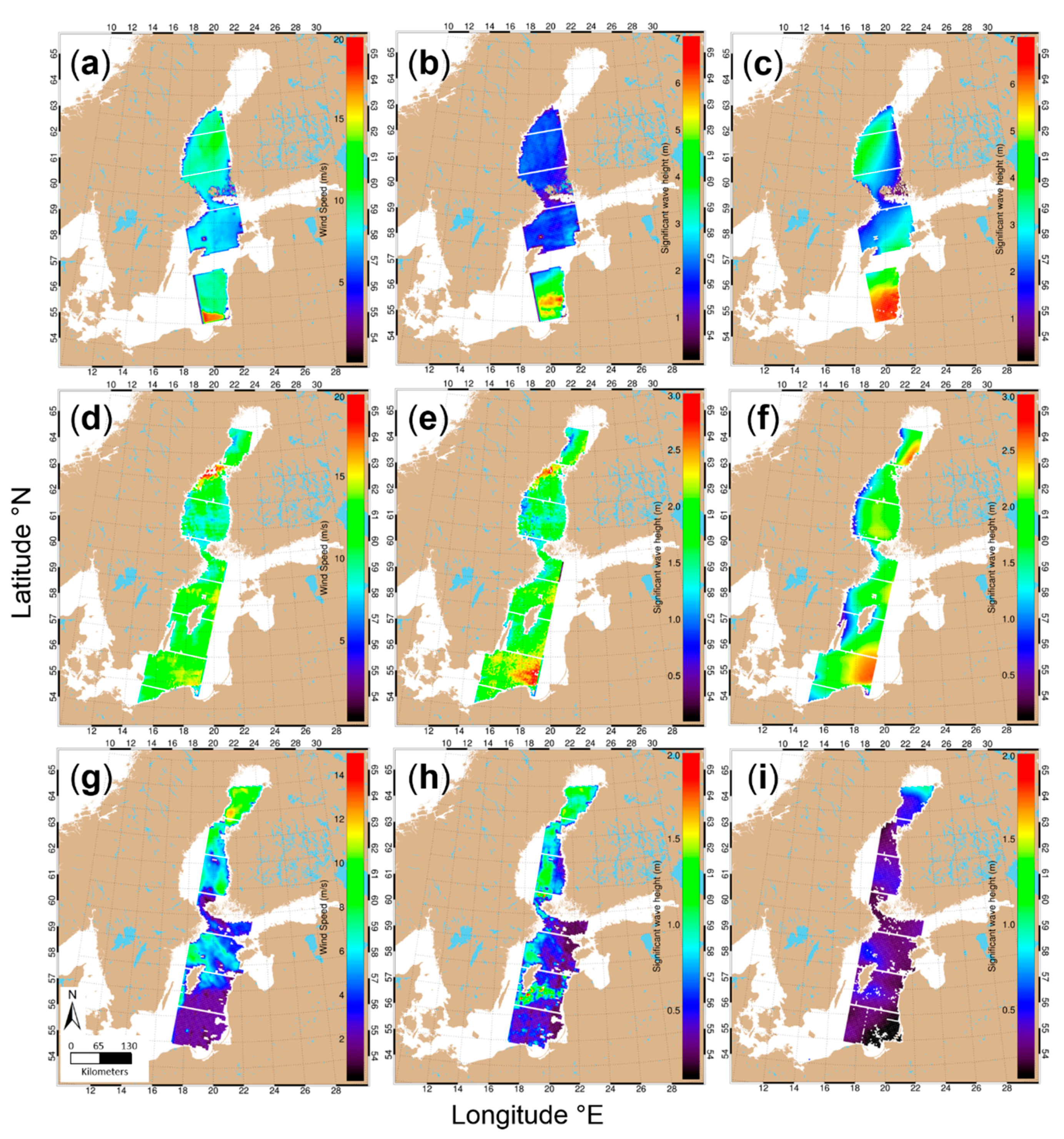
A high sea state example from 11 January 2015 (16:19 UTC) is presented in Figure 4a–c. Considering the general Baltic Sea wave conditions, high significant wave height values (up to 7.5 m) were observed along the Polish and Lithuanian coasts. Both the SAR-derived results and WAM model field show good general agreement in the wave height values and location of maximum (r = 0.91). The area of the storm on the SAR image is smaller and does not spread as much to the north as in the WAM results. The maximum significant wave height from SAR is about 0.5 m higher (Figure 4b, Table 4). Another region with some differences between the wave fields retrieved with the two different methods is seen in the Bothnia Sea area, where SAR-derived wave height along the Swedish coast is about two meters lower compared to the model data.
The second example depicts medium sea state conditions in the Baltic Proper and the Gulf of Bothnia on 2 October 2015 (Figure 4d–f). Again, a good general match between wave fields (considering the wave height and spatial pattern) estimated from SAR data and the WAM model outcome can be observed. SAR-derived wave height field is more variable (STD from 1.14 m to 1.51 m) than the model field (STD from 0.17 m to 1.48 m), which is the case for all examples (Table 4). Also, there are some differences in the wave field pattern along the Swedish coast where the wave height is underestimated by WAM model data compared to SAR-derived fields.
Most commonly occurring, the low sea state [19] example on 5 July 2015 over the Baltic Sea (HS is around 1 m) is presented in Figure 4g–i. Although WAM wave model results are smoother and lower than SAR-derived values, they represent a very similar large-scale pattern. One can notice the increased wave height values to the north and to the south of Gotland Island. A similar pattern from both datasets is also observed in Bothnia Sea region. The low sea state conditions might not be the most relevant from a safe navigation point of view and operational monitoring/forecasting of the wave conditions is not as critical as during storm conditions. Nevertheless, it is still relevant for routine environmental monitoring and therefore noteworthy that during the low sea state, most of the wave field variability is lost in the model outcome compared to SAR-derived values. A similar example from TerraSAR-X satellite data is presented in Rikka et al. [21], where during low sea state conditions the local wave height increases by 0.5–1 m in kilometre-size “islands” (small local area with elevated wave height values). In Sentinel-1A/B (Figure 4g–i), the size of the observed “island” is larger due to larger SAR resolution and processing grid step which does not allow retrieving such fine scale variations as in the case of TerraSAR-X data. Similarly, Romeiser et al. [41] showed that in hurricane situations, the wavelength is analogously retrieved in island-like fashion from C-band satellite radar.
The case studies showed good general agreement between the SAR-derived and WAM model wave fields. However, there are some differences between the results obtained with the two methods: (i) the area and the location of the storm might be different; (ii) the wave height variability of WAM model fields is lower compared to the SAR-derived fields. The variation in WAM model fields is lost mostly due to wind forcing fields (HIRLAM) used in the wave modelling which have 1 h temporal resolution and 11 km spatial resolution. Therefore, the forcing fields do not include local fine-scale wind field variations and gusts that influence the radar backscatter and related wave field pattern on SAR imagery.
5. Discussion
The current study, as well as previous studies [13,15,21,22,23,24,25] demonstrate the advantages of SAR data in general and Sentinel-1 A/B IW data in particular for the operational sea state monitoring (downstream) services. The meteo-marine parameters derived from Sentinel-1 A/B IW data provide added value to operational monitoring/forecasting services (NRT open source data with high spatial resolution and large spatial coverage; frequency of acquisitions) and statistical analysis (large dataset with sufficient spatial coverage in the coastal zone). Together with the unrestricted access to operational in situ data collected by various Baltic Sea countries and model forecast (e.g., CMEMS, BOOS), the SAR-derived meteo-marine parameters form a basis for improving maritime situation awareness. Furthermore, other applications in the Baltic Sea region, e.g., oil spill detection (impact of wave-wind conditions on detection accuracy), sea ice monitoring (waves under ice), wave-circulation coupling [42], etc. will benefit from incorporation of the Sentinel-1 A/B sea state products in these service chains [29,43].
5.1. Benefits of Sentinel-1A/B IW Wave Field Data for Operational Services
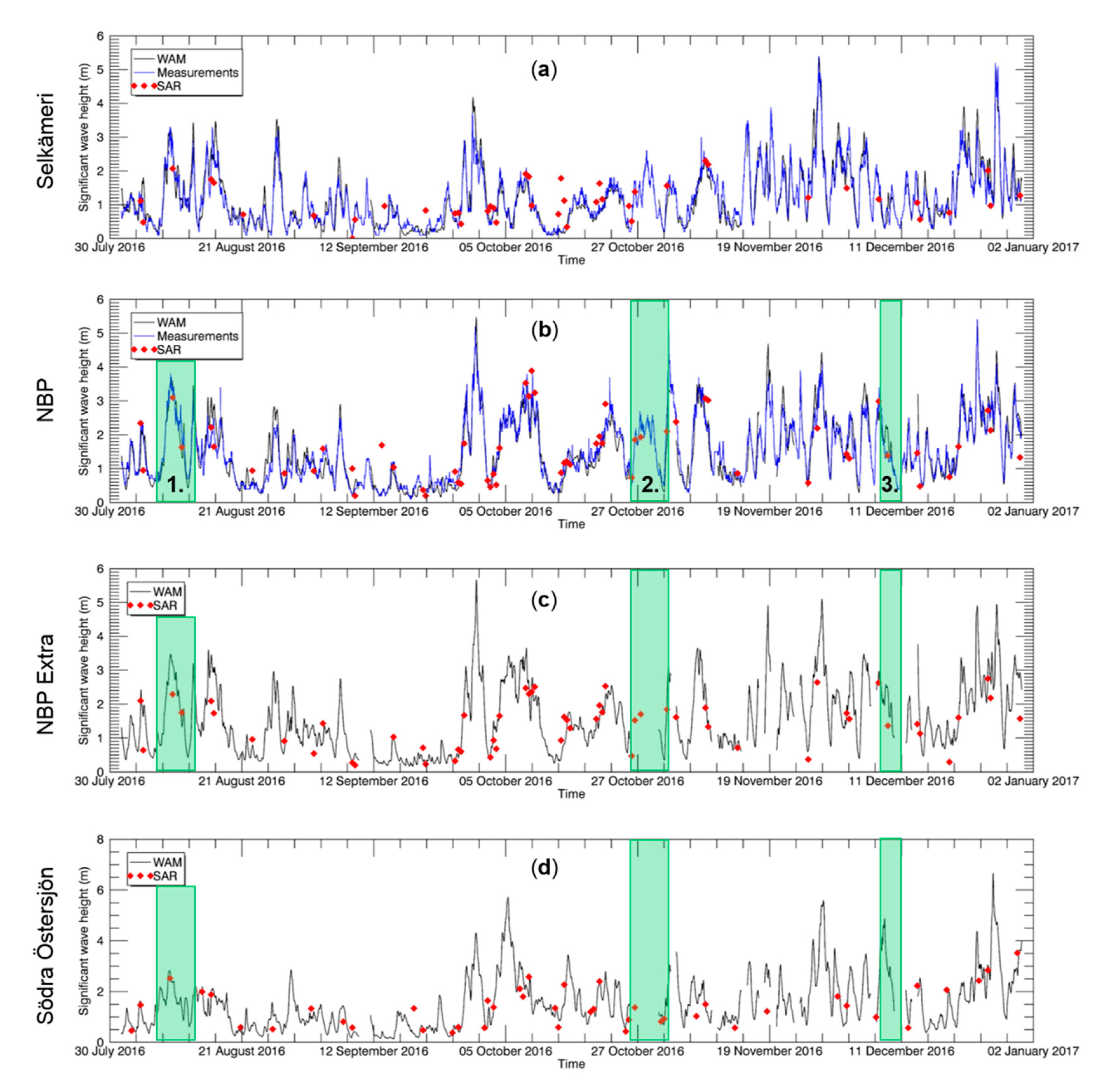
An independent time series from 1 August 2016 until the end of 2016 from four separate locations demonstrate the benefits of using SAR-derived significant wave height retrievals (Figure 5).
In areas where average significant wave height is very low, for example, Selkämeri station in Figure 5a, the SAR-derived results (r = 0.79) are not as accurate as the results over the open part of the Baltic Sea in the NBP station (r = 0.92) on Figure 5b. It is known from previous studies that dominant wave height in the Baltic Sea is around 1 m [19] and relatively low spatial resolution of Sentinel-1 IW mode data might complicate the accurate wave height estimation.
In Figure 5b,c three cases highlighted in green are brought out to explain the benefits of using SAR data. In “case 1” of Figure 5b, one can observe that both WAM wave model results and SAR-derived results match closely with the in situ measurements of the NBP station. However, in Figure 5c which represents a location 60 km away from NBP, a mismatch between SAR and WAM results can be seen in the “case 1” region. The reason could be that since SAR represents better detailed spatial variability/pattern, the actual significant wave height was lower than WAM had predicted at the specific time and location. “Case 3” in Figure 5b,c shows good general match between in situ measurements, SAR-derived wave height, and WAM output in separate places, suggesting that the wave field was spatially more uniform. In general, SAR-derived results could be used as validation data for wave models.
Since the Baltic Sea is seasonally ice-covered, in situ measurement devices are removed for the winter period. Similarly, when the buoys have technical problems (e.g., no data connection) or during their maintenance, highly valuable information is lost. Moreover, wave models may also have short periods with technical problems when no wave forecast is provided. These situations can be observed in “case 2” in Figure 5c, where SAR-derived results become the only source of wave information.
Figure 5d demonstrates the added benefit of using SAR data to retrieve wave information over the poorly sampled area. Although Södra Östersjön station (55.9167°N, 18.7833°E) is included into BOOS measurement stations, the last unrestricted access measurement data was received in 2011. However, Southern Baltic Sea is a location where the highest waves occur [18,19]. As no in situ measurements are carried out in the region, the SAR-derived results would be highly valuable for model validation and/or assimilation into the wave model.
5.2. Statistical Mapping of Coastal/Regional Wave Field: Comparison with Altimetry
Although Sentinel-1A/B are not able to cover the extent of the Baltic Sea (or any sea in that matter) as frequently as wave models can, the SAR data can be as valuable as any other satellite-based wave product (e.g., altimetry products). Altimetry products validations have shown reliable performance (RMSE less than 0.5 m) in the open ocean [44,45,46,47] and in the coastal sea (RMSE up to 0.37 m) [48,49,50,51,52]. However, the spatial coverage of altimetry products is limited and restricted to offshore areas (30–70 km from coast) [53]. The low-resolution altimetry wave products/algorithms and open ocean SAR wave mode products (not available for the coastal areas, including Baltic Sea) are not sufficient for local and regional applications in the complex coastal environment, such as Baltic Sea. The sea state products derived from Sentinel-1 SAR IW data provide information over a large area, including the coastal zone with similar product accuracy (r = 0.88, RMSE = 0.40 m, Table 3) to the altimetry products. Thus, the high-resolution SAR wave data would provide added value for user communities dealing with coastal processes. Moreover, SAR wave products enable to resolve detailed spatial variability while in situ data describes detailed temporal variability in a limited number of locations (Figure 4 and Figure 5).
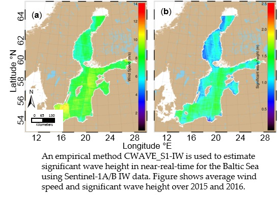
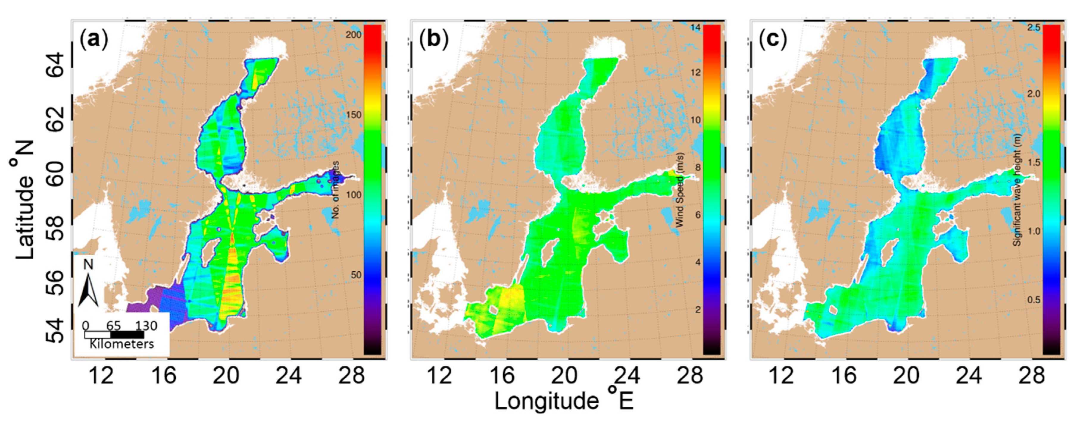
Besides NRT, an example of SAR data benefits is the statistical analysis of wave conditions (e.g., wave climate). Figure 6 represents the average wind speed and significant wave height values from Sentinel-1A/B IW data over the 2015 and 2016 interpolated onto WAM wave model grid. The average significant wave height values over the two-year period (Figure 6c) generally represent similar values to previous studies that used either model data reanalysis or altimetry products over a longer period (up to 23 years) (e.g., Figure 6 in Tuomi et al. [19]; Figure 2 in Kudryavtseva et al. [54]). There are clearly higher average wave height values in the open parts of the Baltic Sea (around 1.8 m) and lower values in the Gulf of Riga (up to 1.0 m in the open part; below 0.8 m in the coastal areas) or the Bothnian Sea (from 0.7 m to 1.2 m). However, from Figure 6a we can conclude that more than 100 points would be necessary for calculating average values since a limited number of samples may cause artificial features and improbable wind speed/wave height fields (e.g., in Southern Baltic Sea (Figure 6b). Considering the long-term objectives of the Copernicus program and the revisit cycle of the Sentinel-1 mission, the statistical bases for wave mapping will improve over time.
Compared to altimetry, SAR data have a benefit of much higher resolution and larger coverage. For example, Kudryavtseva et al. [54] calculated average significant wave height maps for the Baltic Sea over the period of 23 years using approximately 660,000 data points with the end-resolution of 0.2 × 0.1°. To retrieve the analogous map from SAR data, over 3 billion data points can be obtained from a two year period (using the 3 nm processing step). Furthermore, SAR data provides much greater detail, especially in the coastal zones where the vicinity of the coastline influences the altimetry signal and the related wave height retrievals.
6. Conclusions
A method for sea state parameter and marine wind estimation from Sentinel-1 IW SAR imagery in the Baltic Sea (proposed by Pleskachevsky et al. [20]) was validated. The sea state parameters were retrieved from image spectrum using an empirical algorithm CWAVE_S1-IW to estimate integrated sea state parameters directly from SAR image spectra without transformation into wave spectra. The study shows that wave field retrievals from Sentinel-1 IW SAR data correlate with in situ data (r = 0.88, RMSE = 0.40) as well as with WAM wave model (r = 0.86, RMSE = 0.47). Furthermore, the wind speed retrievals that were derived with the CMOD algorithm correlated with the values recorded at the coastal meteorological stations (r = 0.91, RMSE = 1.43).
The advantages of Sentinel-1 SAR IW mode wave products in Baltic Sea were demonstrated. The free/open data, high spatial resolution, large spatial coverage, and frequent acquisitions of Sentinel-1 A/B IW images leads to the following improvements that Sentinel-1 can offer to operational wave field monitoring and forecasting: (i) improved description of spatial variability of significant wave height; (ii) improved estimation of the area and the location of the storms during high sea state.
Considering the advantages, the operational wave product retrieved from Sentinel-1 A/B IW mode data by a dedicated algorithm for the coastal ocean (including Baltic Sea) would be valuable for many communities dealing with wave modelling, operational monitoring, and forecasting, etc. The SAR wave field retrievals would improve the downstream of monitoring services by improving the forecast accuracy, thus enabling a better understanding of coastal processes.
This work contributes to the uptake of Sentinel-1 A/B IW data in the fully automated operational service for meteo-marine parameter retrieval in the Baltic Sea. Implementation of Sentinel-1 sea state products for assimilation into an operational wave model and usage for model forecast quality checking would improve general marine awareness. All the SAR processing methods presented in the study are running as NRT services in the German Aerospace Center’s (DLR) ground station, Neustrelitz.
Author Contributions
S.R. was responsible for designing the study, processing and analysis of SAR data, interpretation of the results and writing the manuscript; A.P. was responsible for CWAVE_S1-IW method development and contributed in data analysis; S.J. was responsible for method development and contributed in writing the manuscript; V.A. performed wave model experiments and contributed in writing the paper; R.U. contributed in interpretation of results and writing the paper.
Acknowledgments
The authors express the gratitude towards ESA for making Sentinel constellation data freely available. Special thanks to Finnish Meteorological Institute (FMI), Swedish Meteorological and Hydrological Institute (SMHI), Estonian Environmental Agency (KAUR), and Latvian Environment, Geology and Meteorology Centre that have open data policy for wind and wave measurement data. We would also like to thank colleagues T. Kõuts, U. Lips, and K. Vahter at Department of Marine Systems at TUT for providing wave and wind measurement data. The authors are grateful for the DLR ground station Neustrelitz team for continuous cooperation and organization of the NRT services for the users. The corresponding author gratefully acknowledges the European Regional Development Fund for financial support for the stay in DLR’s SAR Oceanography group. The author would also like to thank for the warm welcome by the SAR Oceanography group and the exceedingly qualified knowledge shared by them in various SAR-related subjects. The study was supported by institutional research funding IUT (19-6), by Personal Research Funding PUT1378 of the Estonian Ministry of Education and Research, by the European Regional Development Fund and through CMEMS Copernicus grant WAVE2NEMO.
Conflicts of Interest
The authors declare no conflict of interest.
References
- Lehner, S.; Schulz-Stellenfleth, J.; Brusch, S.; Li, X.M. Use of TerraSAR-X data for oceanography. In Proceedings of the 2008 7th European Conference on Synthetic Aperture Radar (EUSAR), Rome, Italy, 26–30 May 2008; pp. 1–4. [Google Scholar]
- Li, X.; Lehner, S.; Rosenthal, W. Investigation of ocean surface wave refraction using TerraSAR-X data. IEEE Trans. Geosci. Remote Sens. 2010, 48, 830–840. [Google Scholar]
- Beal, R.C.; Tilley, D.G.; Monaldo, F.M. Large-And Small-Scale Spatial Evolution of Digitally Processed Ocean Wave Spectra from SEASAT Synthetic Aperture Radar. J. Geophys. Res. Oceans 1983, 88, 1761–1778. [Google Scholar] [CrossRef]
- Masuko, H.; Okamoto, K.I.; Shimada, M.; Niwa, S. Measurement of Microwave Backscattering Signatures of the Ocean Surface Using X Band and Ka Band Airborne Scatterometers. J. Geophys. Res. Oceans 1986, 91, 13065–13083. [Google Scholar] [CrossRef]
- Schulz-Stellenfleth, J. Ocean Wave Measurements Using Complex Synthetic Aperture Radar Data; University of Hamburg: Hamburg, Germany, 2004. [Google Scholar]
- Hasselmann, K.; Hasselmann, S. On the Nonlinear Mapping of an Ocean Wave Spectrum into a Synthetic Aperture Radar Image Spectrum and Its Inversion. J. Geophys. Res. Oceans 1991, 96, 10713–10729. [Google Scholar] [CrossRef]
- Hasselmann, S.; Brüning, C.; Hasselmann, K.; Heimbach, P. An Improved Algorithm for the Retrieval of Ocean Wave Spectra from Synthetic Aperture Radar Image Spectra. J. Geophys. Res. Oceans 1996, 101, 16615–16629. [Google Scholar] [CrossRef]
- Schulz-Stellenfleth, J.; Lehner, S.; Hoja, D. A Parametric Scheme for the Retrieval of Two-Dimensional Ocean Wave Spectra from Synthetic Aperture Radar Look Cross Spectra. J. Geophys. Res. Oceans 2005, 110, C05004. [Google Scholar] [CrossRef]
- Alpers, W.R.; Ross, D.B.; Rufenach, C.L. On the Detectability of Ocean Surface Waves by Real and Synthetic Aperture Radar. J. Geophys. Res. Oceans 1981, 86, 6481–6498. [Google Scholar] [CrossRef]
- Lyzenga, D.R. Unconstrained Inversion of Waveheight Spectra from SAR Images. IEEE Trans. Geosci. Remote Sens. 2002, 40, 261–270. [Google Scholar] [CrossRef]
- Bruck, M. Sea State Measurements Using TerraSAR-X/TanDEM-X Data; Christian-Albrechts-Universität zu Kiel: Kiel, Germany, 2015. [Google Scholar]
- Li, X.M.; Lehner, S.; Bruns, T. Ocean Wave Integral Parameter Measurements Using ENVISAT ASAR Wave Mode Data. IEEE Trans. Geosci. Remote Sens. 2011, 49, 155–174. [Google Scholar] [CrossRef] [Green Version]
- Pleskachevsky, A.L.; Rosenthal, W.; Lehner, S. Meteo-Marine Parameters for Highly Variable Environment in Coastal Regions from Satellite Radar Images. ISPRS J. Photogr. Remote Sens. 2016, 119, 464–484. [Google Scholar] [CrossRef]
- Schulz-Stellenfleth, J.; König, T.; Lehner, S. An Empirical Approach for the Retrieval of Integral Ocean Wave Parameters from Synthetic Aperture Radar Data. J. Geophys. Res. Oceans 2007, 112, C03019. [Google Scholar] [CrossRef]
- Stopa, J.E.; Mouche, A. Significant wave heights from Sentinel-1 SAR: Validation and applications. J. Geophys. Res. Oceans 2017, 122, 1827–1848. [Google Scholar] [CrossRef]
- Schwarz, E.; Krause, D.; Berg, M.; Daedelow, H.; Maass, H. Near Real Time Applications for Maritime Situational Awareness. Int. Arch. Photogr. Remote Sens. Spat. Inf. Sci. 2015, 40, 999–1003. [Google Scholar] [CrossRef] [Green Version]
- Soomere, T.; Räämet, A. Spatial Patterns of the Wave Climate in the Baltic Proper and the Gulf of Finland. Oceanologia 2011, 53, 335–371. [Google Scholar] [CrossRef]
- Björkqvist, J.-V.; Lukas, I.; Alari, V.; van Vledder, G.P.; Hulst, S.; Pettersson, H.; Behrens, A.; Männik, A. Comparing a 41-year model hindcast with decades of wave measurements from the Baltic Sea. Ocean Eng. 2018, 152, 57–71. [Google Scholar] [CrossRef]
- Tuomi, L.; Kahma, K.K.; Pettersson, H. Wave hindcast statistics in the seasonally ice-covered Baltic sea. Boreal Environ. Res. 2011, 16, 451–472. [Google Scholar]
- Pleskachevsky, A.; Jacobsen, S.; Tings, B.; Schwarz, E. Sea State from Sentinel-1 Synthetic Aperture Radar Imagery for Maritime Situation Awareness. Int. J. Remote Sens. submitted.
- Rikka, S.; Pleskachevsky, A.; Uiboupin, R.; Jacobsen, S. Sea state in the Baltic Sea from space-borne high-resolution synthetic aperture radar imagery. Int. J. Remote Sens. 2018, 39, 1256–1284. [Google Scholar] [CrossRef]
- Ressel, R.; Singha, S.; Lehner, S.; Rösel, A.; Spreen, G. Investigation into Different Polarimetric Features for Sea Ice Classification Using X-Band Synthetic Aperture Radar. IEEE J. Sel. Top. Appl. Earth Obs. Remote Sens. 2016, 9, 3131–3143. [Google Scholar] [CrossRef] [Green Version]
- Singha, S.; Velotto, D.; Lehner, S. Dual-polarimetric feature extraction and evaluation for oil spill detection: A near real time perspective. In Proceedings of the 2015 IEEE International on Geoscience and Remote Sensing Symposium (IGARSS), Milan, Italy, 26–31 July 2015; pp. 3235–3238. [Google Scholar]
- Velotto, D.; Bentes, C.; Tings, B.; Lehner, S. First Comparison of Sentinel-1 and TerraSAR-X Data in the Framework of Maritime Targets Detection: South Italy Case. IEEE J. Ocean. Eng. 2016, 41, 993–1006. [Google Scholar] [CrossRef]
- Ardhuin, F.; Stopa, J.; Chapron, B.; Collard, F.; Smith, M.; Thomson, J.; Doble, M.; Blomquist, B.; Persson, O.; Collins III, C.O. Measuring ocean waves in sea ice using SAR imagery: A quasi-deterministic approach evaluated with Sentinel-1 and in situ data. Remote Sens. Environ. 2017, 189, 211–222. [Google Scholar] [CrossRef]
- Shao, W.; Zhang, Z.; Li, X.; Li, H. Ocean wave parameters retrieval from Sentinel-1 SAR imagery. Remote Sens. 2016, 8, 707. [Google Scholar] [CrossRef]
- Ardhuin, F.; Chapron, B.; Collard, F. Observation of swell dissipation across oceans. Geophys. Res. Lett. 2009, 36. [Google Scholar] [CrossRef]
- Collard, F.; Ardhuin, F.; Chapron, B. Monitoring and analysis of ocean swell fields from space: New methods for routine observations. J. Geophys. Res. Oceans 2009, 114. [Google Scholar] [CrossRef]
- Tuomi, L.; Vähä-Piikkiö, O.; Alari, V. Baltic Sea Wave Analysis and Forecasting Product BALTICSEA_ANALYSIS_FORECAST_WAV_003_010; Issue 1.0, CMEMS, 2017. [Google Scholar]
- Tuomi, L.; Vähä-Piikkiö, O.; Alari, V. CMEMS Baltic Monitoring and Forecasting Centre: High-resolution wave forecast in the seasonally ice-covered Baltic Sea. In Proceedings of the 8th International EuroGOOS Conference, Bergen, Norway, 3–5 October 2017. [Google Scholar]
- Von Schuckmann, K.; Le Traon, P.-Y.; Alvarez-Fanjul, E.; Axell, L.; Balmaseda, M.; Breivik, L.-A.; Brewin, R.J.; Bricaud, C.; Drevillon, M.; Drillet, Y.; et al. The Copernicus marine environment monitoring service ocean state report. J. Oper. Ocean. 2016, 9, s235–s320. [Google Scholar] [CrossRef]
- Group, T.W. The WAM model—A third generation ocean wave prediction model. J. Phys. Ocean. 1988, 18, 1775–1810. [Google Scholar] [CrossRef]
- Whitham, G.B. Linear and Nonlinear Waves; John Wiley & Sons: New York, NY, USA, 1974. [Google Scholar]
- Stoffelen, A.; Anderson, D. Scatterometer data interpretation: Estimation and validation of the transfer function CMOD4. J. Geophys. Res. Oceans 1997, 102, 5767–5780. [Google Scholar] [CrossRef]
- Hersbach, H.; Stoffelen, A.; de Haan, S. An improved C-band scatterometer ocean geophysical model function: CMOD5. J. Geophys. Res. Oceans 2007, 112. [Google Scholar] [CrossRef]
- Monaldo, F.; Jackson, C.; Li, X.; Pichel, W.G. Preliminary evaluation of Sentinel-1A wind speed retrievals. IEEE J. Sel. Top. Appl. Earth Obs. Remote Sens. 2016, 9, 2638–2642. [Google Scholar] [CrossRef]
- Thompson, D.R.; Elfouhaily, T.M.; Chapron, B. Polarization ratio for microwave backscattering from the ocean surface at low to moderate incidence angles. In Proceedings of the 1998 IEEE International on Geoscience and Remote Sensing Symposium (IGARSSS’98), Seattle, WA, USA, 6–10 July 1998; pp. 1671–1673. [Google Scholar]
- Horstmann, J.; Falchetti, S.; Wackerman, C.; Maresca, S.; Caruso, M.J.; Graber, H.C. Tropical cyclone winds retrieved from C-band cross-polarized synthetic aperture radar. IEEE Trans. Geosci. Remote Sens. 2015, 53, 2887–2898. [Google Scholar] [CrossRef]
- Skamarock, W.C.; Klemp, J.B.; Dudhia, J.; Gill, D.O.; Barker, D.M.; Wang, W.; Powers, J.G. A Description of the Advanced Research WRF Version 2 (No. NCAR/TN-468+ STR); National Center For Atmospheric Research Boulder Co Mesoscale and Microscale Meteorology Div: Boulder, CO, USA, 2005. [Google Scholar]
- Haralick, R.M.; Shanmugam, K. Textural Features for Image Classification. IEEE Trans. Syst. Man Cyber. 1973, 3, 610–621. [Google Scholar] [CrossRef]
- Romeiser, R.; Graber, H.C.; Caruso, M.J.; Jensen, R.E.; Walker, D.T.; Cox, A.T. A new approach to ocean wave parameter estimates from C-band ScanSAR images. IEEE Trans. Geosci. Remote Sens. 2015, 53, 1320–1345. [Google Scholar] [CrossRef]
- Alari, V.; Staneva, J.; Breivik, Ø.; Bidlot, J.-R.; Mogensen, K.; Janssen, P. Response of water temperature to surface wave effects in the Baltic Sea: Simulations with the coupled NEMO-WAM model. In Proceedings of the EGU General Assembly Conference Abstracts, Vienna Austria, 17–22 April 2016; p. 4363. [Google Scholar]
- European Maritime Safety Agency. EMSA CleanSeaNet First Generation Report; EMSA: Lisboa, Portugal, 2011. [Google Scholar]
- Ducet, N.; Le Traon, P.-Y.; Reverdin, G. Global high-resolution mapping of ocean circulation from TOPEX/Poseidon and ERS-1 and-2. J. Geophys. Res. Oceans 2000, 105, 19477–19498. [Google Scholar] [CrossRef]
- Pascual, A.; Faugère, Y.; Larnicol, G.; Le Traon, P.Y. Improved description of the ocean mesoscale variability by combining four satellite altimeters. Geophys. Res. Lett. 2006, 33. [Google Scholar] [CrossRef]
- Pujol, M.-I.; Faugère, Y.; Taburet, G.; Dupuy, S.; Pelloquin, C.; Ablain, M.; Picot, N. DUACS DT2014: The new multi-mission altimeter data set reprocessed over 20 years. Ocean Sci. 2016, 12, 1067–1090. [Google Scholar] [CrossRef]
- Ray, R.D.; Beckley, B. Simultaneous ocean wave measurements by the Jason and Topex satellites, with buoy and model comparisons special issue: Jason-1 calibration/Validation. Mar. Geod. 2003, 26, 367–382. [Google Scholar] [CrossRef]
- Bouffard, J.; Vignudelli, S.; Cipollini, P.; Menard, Y. Exploiting the potential of an improved multimission altimetric data set over the coastal ocean. Geophys. Res. Lett. 2008, 35. [Google Scholar] [CrossRef] [Green Version]
- Cazenave, A.; Bonnefond, P.; Mercier, F.; Dominh, K.; Toumazou, V. Sea level variations in the Mediterranean Sea and Black Sea from satellite altimetry and tide gauges. Glob. Plan. Chang. 2002, 34, 59–86. [Google Scholar] [CrossRef]
- Kudryavtseva, N.A.; Soomere, T. Validation of the multi-mission altimeter wave height data for the Baltic Sea region. arXiv, 2016; arXiv:1603.08698. [Google Scholar]
- Madsen, K.S.; Høyer, J.; Tscherning, C.C. Near-coastal satellite altimetry: Sea surface height variability in the North Sea–Baltic Sea area. Geophys. Res. Lett. 2007, 34. [Google Scholar] [CrossRef]
- Vignudelli, S.; Cipollini, P.; Roblou, L.; Lyard, F.; Gasparini, G.; Manzella, G.; Astraldi, M. Improved satellite altimetry in coastal systems: Case study of the Corsica Channel (Mediterranean Sea). Geophys. Res. Lett. 2005, 32. [Google Scholar] [CrossRef]
- Høyer, J.L.; Nielsen, J. Satellite significant wave height observations in coastal and shelf seas. In Proceedings of the Symposium on 15 Years of Progress in Radar Altimetry, Venice, Italy, 13–18 March 2006. [Google Scholar]
- Kudryavtseva, N.; Soomere, T. Satellite altimetry reveals spatial patterns of variations in the Baltic Sea wave climate. arXiv, 2017; arXiv:1705.01307. [Google Scholar]
Figure 1.
Sentinel-1A/B IW relative orbit overlays and corresponding orbit numbers over the Baltic Sea. (a) ascending/morning orbits and (b) descending orbits in the evenings.
Figure 1.
Sentinel-1A/B IW relative orbit overlays and corresponding orbit numbers over the Baltic Sea. (a) ascending/morning orbits and (b) descending orbits in the evenings.

Figure 2.
The map of the Baltic Sea and locations of measurement stations used in the study. The location of wave measurements—significant wave height, wave propagation direction, wave period (red), and coastal wind measurements—speed, gusts, direction (blue) are indicated on the map; green marks extra stations (virtual buoys).

Figure 3.
(a) Scatterplot for sea state for available collocated data acquired over the Baltic Sea including 15 Sentinel-1A/B scenes (overflights/events/days) with 116 individual Sentinel-1 IW mode images and 52 buoy collocations. The correlation coefficient between SAR and in situ measurements is 0.88, RMSE is 0.40 m, and Scatter Index is 0.37. (b) Scatterplot for surface wind speed for all available collocated data acquired over the Baltic Sea. The correlation coefficient r is 0.91, RMSE is 1.43 m s−1, and SI is 0.19. (c) Histogram plot for all the collocated SAR versus WAM results. The bin size for histogram calculations is 0.2 m. The statistics between the datasets are as follows: r = 0.86, RMSE = 0.47 m, and SI = 0.33.

Figure 4.
Examples of spatially collocated SAR wind (a,d,g) fields, SAR wave fields (b,e,h) and WAM wave fields (c,f,i) during three characteristic situations over the Baltic Sea: high sea state on 11 January 2015 at 16:19 (a–c), medium sea state on 2 October 2015 at 04:56 (d–f) and low sea state on 5 July 2015 at 04:56 (g–i)).

Figure 5.
A timeseries from 1 August 2016 until the end of 2016 from four stations. Two stations—Selkämeri and NBP (Figure 2, Table 1)—include all the data: measurement, WAM, and SAR-derived results; other two stations—NBP Extra (58.7500°N, 20.8271°E; no. 6 in Figure 2) and Södra Östersjön (55.9167°N, 18.7833°E; no. 7 in Figure 2) include WAM result and SAR-derived significant wave height. Highlighted areas indicate some benefits of using SAR data over the Baltic Sea: “case 1” and “case 3” bring out the variability aspect of SAR-derived values whereas “case 2” shows missing measurements that can be replaced with SAR data.

Figure 6.
(a) Number of SAR points; (b) average wind speed; and (c) average significant wave height over 2015–2016 interpolated to WAM model grid.
Figure 6.
(a) Number of SAR points; (b) average wind speed; and (c) average significant wave height over 2015–2016 interpolated to WAM model grid.


Table 1.
Overview of wave measurements used in the study. HS represents total significant wave height.
Table 1.
Overview of wave measurements used in the study. HS represents total significant wave height.
| No. (Origin) | Station | Lat (°N) | Lon (°E) | Sensor | Data Used |
|---|---|---|---|---|---|
| 1 (FIN) | Selkämeri | 61.8001 | 20.2327 | Waverider | HS |
| 2 (SWE) | Finngrundet | 61.0000 | 18.6667 | Waverider | HS |
| 3 (FIN) | NBP | 59.2500 | 20.9968 | Waverider | HS |
| 4 (EST) | Vilsandi | 58.4889 | 21.6333 | Waverider | HS |
| 5 (SWE) | Knolls grund | 57.5167 | 17.6167 | Waverider | HS |
| 6 | NBP Extra | 58.7500 | 20.8271 | Virtual buoy | HS |
| 7 | Södra Östersjön | 55.9167 | 18.7833 | Virtual buoy | HS |
Table 2.
Sentinel-1A/B acquisitions used for the study. Relative orbit numbers with acquisitions per scene are listed. Mean and maximum significant wave height and wind speed calculated with the methods described in Section 3 are shown with the number of collocations per overpasses.
Table 2.
Sentinel-1A/B acquisitions used for the study. Relative orbit numbers with acquisitions per scene are listed. Mean and maximum significant wave height and wind speed calculated with the methods described in Section 3 are shown with the number of collocations per overpasses.
| Sentinel-1 UTC | Relative Orbit no. | Images in Scene | Mean/Max HS per Scene | Mean/Max U10 per Scene | Collocations (Wave/Wind) |
|---|---|---|---|---|---|
| 11 January 2015 16:19 | 29 | 6 | 2.4/7.5 | 9.0/18.7 | 3/11 |
| 22 April 2015 16:28 | 102 | 6 | 0.3/1.7 | 2.6/11.8 | 2/3 |
| 04 June 2015 05:04 | 22 | 9 | 0.9/2.8 | 5.3/14.0 | 4/32 |
| 11 June 2015 04:56 | 124 | 9 | 0.6/2.1 | 4.1/11.5 | 5/28 |
| 25 June 2015 04:56 | 124 | 8 | 0.8/1.8 | 5.1/13.8 | 5/27 |
| 28 June 2015 05:04 | 22 | 9 | 0.6/2.2 | 3.4/8.7 | 4/25 |
| 05 July 2015 04:56 | 124 | 9 | 0.7/2.5 | 4.7/12.4 | 4/22 |
| 28 July 2015 04:56 | 124 | 9 | 0.9/2.4 | 6.6/14.4 | 5/25 |
| 08 August 2015 05:04 | 22 | 9 | 1.7/2.9 | 10.8/16.0 | 4/31 |
| 08 September 2015 16:19 | 29 | 6 | 1.3/2.7 | 8.5/17.3 | 3/19 |
| 02 October 2015 05:04 | 22 | 9 | 1.8/3.6 | 11.6/19.1 | 4/32 |
| 02 October 2015 16:19 | 29 | 5 | 2.5/4.8 | 13.2/18.2 | 1/16 |
| 02 November 2015 04:56 | 124 | 9 | 1.6/2.4 | 10.7/17.1 | 5/32 |
| 09 August 2016 16:19 | 29 | 6 | 1.9/3.7 | 9.7/13.8 | 1/28 |
| 14 December 2016 04:56 | 124 | 7 | 1.4/2.6 | 8.6/13.9 | 2/26 |
| 15 | 116 | 52/357 |
Table 3.
Overview of inter-comparison of significant wave height and wind speed: correlation coefficient (r), root mean square error (RMSE), scatter index (SI), and number of collocations (n). The values in brackets in the 3rd column represent the statistics when all collocated data of Synthetic Aperture Radar (SAR) and wave model (WAM) wave fields were used (49,315 colocations).
| Parameter | SAR vs. In SituWave Height | SAR vs. WAM Wave Height | SAR vs. In Situ Wind Speed | WAM vs. In Situ Wave Height |
|---|---|---|---|---|
| r | 0.88 | 0.81 (0.86) | 0.91 | 0.89 |
| RMSE | 0.40 | 0.47 (0.47) | 1.43 | 0.39 |
| SI | 0.37 | 0.42 (0.33) | 0.19 | 0.36 |
| n | 52 | 52 (49314) | 357 | 52 |
Table 4.
Statistics between Sentinel-1 HS retrievals and WAM numerical model outputs.
| Time UTC | Variable | Sentinel-1 | WAM |
|---|---|---|---|
| 11 January 2015 16:19:22 High sea state | Mean (m) | 2.41 | 3.02 |
| Maximum (m) | 7.47 | 6.97 | |
| STD (m) | 1.51 | 1.48 | |
| r | 0.91 | ||
| RMSE (m) | 1.02 | ||
| 02 October 2015 05:04:47 Medium sea state | Mean (m) | 1.82 | 1.68 |
| Maximum (m) | 3.62 | 2.65 | |
| STD (m) | 1.32 | 0.57 | |
| r | 0.51 | ||
| RMSE (m) | 0.39 | ||
| 05 May 2015 04:56:28 Low sea state | Mean (m) | 0.57 | 0.33 |
| Maximum (m) | 1.84 | 1.02 | |
| STD (m) | 1.14 | 0.17 | |
| r | 0.51 | ||
| RMSE (m) | 0.41 | ||
© 2018 by the authors. Licensee MDPI, Basel, Switzerland. This article is an open access article distributed under the terms and conditions of the Creative Commons Attribution (CC BY) license (http://creativecommons.org/licenses/by/4.0/).
Share and Cite
MDPI and ACS Style
Rikka, S.; Pleskachevsky, A.; Jacobsen, S.; Alari, V.; Uiboupin, R. Meteo-Marine Parameters from Sentinel-1 SAR Imagery: Towards Near Real-Time Services for the Baltic Sea. Remote Sens. 2018, 10, 757. https://doi.org/10.3390/rs10050757
AMA Style
Rikka S, Pleskachevsky A, Jacobsen S, Alari V, Uiboupin R. Meteo-Marine Parameters from Sentinel-1 SAR Imagery: Towards Near Real-Time Services for the Baltic Sea. Remote Sensing. 2018; 10(5):757. https://doi.org/10.3390/rs10050757
Chicago/Turabian StyleRikka, Sander, Andrey Pleskachevsky, Sven Jacobsen, Victor Alari, and Rivo Uiboupin. 2018. "Meteo-Marine Parameters from Sentinel-1 SAR Imagery: Towards Near Real-Time Services for the Baltic Sea" Remote Sensing 10, no. 5: 757. https://doi.org/10.3390/rs10050757
Note that from the first issue of 2016, this journal uses article numbers instead of page numbers. See further details here.