Article

Scratching Beneath the Surface: A Model to Predict the Vertical Distribution of Prochlorococcus Using Remote Sensing

by
Priscila K. Lange
1,*,
Robert J. W. Brewin
2,3,
Giorgio Dall’Olmo
2,3,
Glen A. Tarran
2,
Shubha Sathyendranath
2,3,
Mikhail Zubkov
4 and
Heather A. Bouman
1
1
Department of Earth Sciences, University of Oxford, South Parks Rd, OX1 3AN Oxford, UK
2
Plymouth Marine Laboratory, Prospect Place, The Hoe, PL1 3DH Plymouth, UK
3
National Centre for Earth Observation, Plymouth Marine Laboratory, PL1 3DH Plymouth, UK
4
National Oceanography Centre Southampton, Waterfront Campus, SO14 3ZH Southampton, UK
*
Author to whom correspondence should be addressed.
Remote Sens. 2018, 10(6), 847; https://doi.org/10.3390/rs10060847
Submission received: 27 April 2018 / Revised: 18 May 2018 / Accepted: 18 May 2018 / Published: 29 May 2018
(This article belongs to the Special Issue Remote Sensing of Ocean Colour)

Abstract

:
The unicellular cyanobacterium Prochlorococcus is the most dominant resident of the subtropical gyres, which are considered to be the largest biomes on earth. In this study, the spatial and temporal variability in the global distribution of Prochlorococcus was estimated in the Atlantic Ocean using an empirical model based on data from 13 Atlantic Meridional Transect cruises. Our model uses satellite-derived sea surface temperature (SST), remote-sensing reflectance at 443 and 488 nm, and the water temperature at a depth of 200 m from Argo data. The model divides the population of Prochlorococcus into two groups: ProI, which dominates under high-light conditions associated with the surface, and ProII, which favors low light found near the deep chlorophyll maximum. ProI and ProII are then summed to provide vertical profiles of the concentration of Prochlorococcus cells. This model predicts that Prochlorococcus cells contribute 32 Mt of carbon biomass (7.4 × 1026 cells) to the Atlantic Ocean, concentrated mainly within the subtropical gyres (35%) and areas near the Equatorial Convergence Zone (30%). When projected globally, 3.4 × 1027 Prochlorococcus cells represent 171 Mt of carbon biomass, with 43% of this global biomass allocated to the upper ocean (0–45 m depth). Annual cell standing stocks were relatively stable between the years 2003 and 2014, and the contribution of the gyres varies seasonally as gyres expand and contract, tracking changes in light and temperature, with lowest cell abundances during the boreal and austral winter (1.4 × 10¹³ cells m−2), when surface cell concentrations were highest (9.8 × 10⁴ cells mL−1), whereas the opposite scenario was observed in spring–summer (2 × 10¹³ cells m−2). This model provides a three-dimensional view of the abundance of Prochlorococcus cells, revealing that Prochlorococcus contributes significantly to total phytoplankton biomass in the Atlantic Ocean, and can be applied using either in situ measurements at the sea surface (r2 = 0.83) or remote-sensing observables (r2 = 0.58).

Graphical Abstract

1. Introduction

Until the early 1980s, the largest biomes on our planet, referred collectively as the subtropical gyres [1,2,3], were considered to be oceanic deserts as they are characterised by low biological primary productivity [4]. In the central subtropical gyres, extreme high-light conditions and low-nutrient concentrations hamper phytoplankton growth at the sea surface and lead to very low intracellular pigment concentrations [5,6]. Yet, lying beneath this seemingly barren surface layer, a deep chlorophyll maximum (DCM) is commonly observed at depths between 80 to 120 m [7,8]. This peak in pigment concentration is the result of light penetrating sufficiently deep in the water column to reach depths where nutrients are available from deep reservoirs [9]. Cells found at this depth attain net growth by increasing their intracellular pigment concentration to thrive at low-light levels. The DCM is considered a ubiquitous feature of stratified subtropical waters [5,8]. This allocation of pigment biomass at depth makes these gyre biomes more similar to terrestrial savannahs than deserts. Like the subtropical gyres, savannahs have most of their biomass buried below ground, protected from harsh surface conditions [10]. Although the contribution of the DCM to the integrated chlorophyll biomass in the subtropical gyres is significant, it is still low when compared with coastal marine environments and shelf seas [8].
The use of shipboard flow cytometry revolutionised the study of small phytoplankton cells. In 1988, Chisholm, Olson, and colleagues [11] first documented a ubiquitous picocyanobacterium that was indistinguishable from other bacteria using traditional microscopy, but has since been discovered to be the most abundant photosynthetic organism in the oceans—Prochlorococcus. The average abundance of Prochlorococcus cells in subtropical and tropical waters [12,13,14,15,16,17] is roughly the same order of magnitude of most phytoplankton blooms where a single species of alga typically reaches cell abundances of 104–105 cells mL−1 [18]. Despite its minute size and corresponding low intracellular carbon content (~50 fg C cell−1) [19], this single genus is numerically dominant over vast swaths of the global ocean, with global standing stocks in the order of 1027 cells [20,21] and makes an immense contribution to the marine organic carbon pool.
Although the quantification of Prochlorococcus cells by flow cytometry has increased our understanding of the contribution of this cyanobacterium to phytoplankton biomass in the subtropical gyres, data coverage in these vast regions remains poor. Optical sensors mounted on earth-orbiting satellites provide a synoptic view of environmental variables at global scales, including: sea-surface temperature, reflectance of light at various wavebands (remote-sensing reflectance, Rrs), and the photosynthetically-available radiation (visible light) incident on the sea surface [22]. However, the signals observed by satellites are from the sea surface and thus are blind to changes in the physical and biological properties of the ocean beneath the first few tens of metres [23]. To obtain a three-dimensional view of the ocean environment, Argo floats and ocean gliders equipped with sensors of temperature, salinity, and pressure (which determines depth) can be used to provide information on the vertical structure of the water column [24].
The biogeography of Prochlorococcus has been shown to be strongly related to environmental gradients of temperature and light, and inversely correlated to the presence of other phytoplankton groups indicated by the chlorophyll concentration [15,21,25,26]. As Prochlorococcus is the dominant phytoplankter in large areas of the world’s oceans, it is important to be able to predict how its abundance might vary temporally and spatially in response to environmental and climate changes, and to assess seasonal and long-term changes in their biogeochemical cycles, trophic interactions and energy flow in oceanic food webs. To date, estimates of the global standing stock of Prochlorococcus [21] and its distribution in the world’s oceans [20] do not take into account the vertical structure of cell abundance, which is an important feature of their biogeography and tightly coupled with resource gradients (e.g., light and nutrient concentrations) that govern their growth. Ignoring spatio-temporal changes in vertical structure could not only lead to potential errors in their contribution to water-column standing stocks but also hinder our ability to examine the impact of water-column stratification on the vertical partitioning of Prochlorococcus populations. Here, we present an empirical model that exploits two ocean-observing systems (Aqua-MODIS and Argo) to estimate the vertical and horizontal distribution of Prochlorococcus in the Atlantic basin. This approach captures both seasonal and interannual variations in the vertical distribution of Prochlorococcus cells, thus providing a powerful tool to examine the large-scale dynamics of standing stocks and their contribution to the marine organic carbon cycle.

2. Materials and Methods

The Prochlorococcus abundance model estimates the distribution of cells from the surface to the base of the photic zone using information on light penetration in the water column. The vertical distribution of Prochlorococcus has a form similar to the typical profile of primary production, which is determined by light availability and the photosynthetic response of phytoplankton to available light. Recognizing that primary production may indeed have a role in determining the vertical distribution of this genus in the ocean, we have used equations analogous to that of a photosynthesis-irradiance curve [27] to describe the relationship between cell abundance and the percentage of surface irradiance available at each depth z, henceforth referred to as the fractional PAR (fPAR(z)).
Although many subpopulations adapted to different light levels can coexist [25], the model is based on the assumption that there are two distinct populations of Prochlorococcus with distinct photophysiologies: ProI, which dominates under high-light conditions found near the sea surface, and ProII, which has a preference for low-light conditions near the deep chlorophyll maximum (DCM). Vertical profiles of ProI and ProII are estimated from fPAR(z). When these two populations are added, the resulting vertical profile of total Prochlorococcus cells, Prototal(z), peaks above the depth of the DCM (ZDCM).
The series of equations used to estimate the vertical distribution of Prochlorococcus cells relies on information on four parameters that define the magnitude of the vertical profile of cell abundance: Prochlorococcus abundance at the sea surface (Prosurf) and at the deep maximum (Promax), used to calculate ProI and ProII, respectively; the attenuation coefficient for PAR (KdPAR), used to calculate fPAR at each depth; and the depth of the deep chlorophyll maximum ZDCM, used in the calculation of Promax. To estimate these four parameters, we explored their empirical relationships with environmental predictors that can be obtained from ocean observables or estimated using geo-location and time of the year.

2.1. Model Parameterization

Environmental variables that were related to KdPAR, ZDCM, and the growth of Prochlorococcus cells (Prosurf and Promax) include: sea surface temperature (SST), remote-sensing reflectance at 443 (Rrs(443)) and 488 (Rrs(488)) nm, the photosynthetically-available radiation (PAR), the temperature at 200 m estimated from the Argo array (T200), the solar zenith angle at noon (θs), and the day length (DL). The selection of these variables took into consideration some factors known to determine the distribution of this marine cyanobacterium. For example, Prochlorococcus is restricted to warm waters [13,16,20]; therefore, a thermal threshold was used. Additionally, the difference between SST and T200 is here used as a proxy for ocean stratification [28]. Remote-sensing reflectance of solar radiation in the visible domain is inversely related to light absorption by phytoplankton pigments and other light-absorbing substances, such that Rrs(443) and Rrs(488) are closely related to the concentration of chlorophyll at the sea surface. Therefore, the correlation between Rrs(443) and ZDCM is relatively strong, as ZDCM tends to be deeper when there is less chlorophyll at the sea surface [29].
The sea-surface reflectance at blue wavelengths typically increases as the pigment biomass of most phytoplankton decreases (thus reducing light absorption). When the abundance of only Prochlorococcus cells is plotted against Rrs(488) (sr−1), we see that Rrs decreases with an increase in cell abundance, but after a certain threshold is reached, further decrease in Rrs is independent of the abundance of Prochlorococcus, suggesting phytoplankton other than Prochlorococcus might be determining changes in Rrs below this threshold (Figure S8b). The underwater light field is determined by KdPAR in the model, which directly influences ZDCM and the vertical distribution of Prochlorococcus cells. Light availability in the water column is also a function of the DL, which governs the daily integrated irradiance at the sea surface, and θs, which dictates the path length of light per unit of vertical distance within the water column (i.e., lower θs lead to lower light attenuation and a more vertical light path, with light reaching deeper waters). In addition, there is the influence of atmospheric components like aerosols and cloud cover, which limit the incidence of PAR increasing the relative influence of inherent optical properties on the diffusion of light in the water column (i.e., equatorial upwelling regions).
Multilinear relationships between each parameter (KdPAR, ZDCM, Prosurf, and Promax) and the abovementioned environmental variables were examined in a dataset from 13 Atlantic Meridional Transect (AMT) cruises (AMT 12–24) (Figure 1, Table S1) consisting of 704 vertical profiles (8722 observations) which covered a broad area of the Atlantic Ocean. For each cruise, vertical profiles of temperature, chlorophyll fluorescence, and downwelling PAR (British Oceanographic Data Centre—BODC) were measured alongside Prochlorococcus cell counts determined by flow cytometry. Details of the flow-cytometric analysis, the calculation of in situ variables (KdPAR and ZDCM, where the prime denotes in situ data), and programming languages and packages used for all calculations and data management are described in the Suppl. Material. Remote-sensing reflectance data were acquired from matching 8-day composites satellite imagery (Aqua-MODIS) [22].

2.2. Prochlorococcus Abundance Predicted Using Ocean Observables

KdPAR, ZDCM, Prosurf, and Promax were estimated based on their empirical relationships with six environmental variables: SST, Rrs(443), Rrs(488), T200, DL, and θs. SST, Rrs(443) and Rrs(488) were acquired by the satellite Aqua-MODIS and provided by the NASA Ocean Color group [22]. Monthly climatological data of T200 [24] was extracted from Argo vertical temperature profiles. Satellite and Argo data products were regridded to a 4 × 4 km resolution, and every grid cell was used as input data for the Prochlorococcus cell abundance model.
Based on a subset of AMT cruises (Table S2), henceforth called subdataset, a group of variables was selected to predict each parameter using a backward stepwise multilinear regression [30]. The subdataset was randomly resampled allowing repetition of random data to generate the same number of observations as the original subdataset (Monte Carlo test with 2000 bootstrap permutations). In each subdataset, the multilinear relationship between the response and the selected explanatory variables was assessed and algorithm coefficients were computed [31]. The mean of each coefficient distribution was used in our predictive algorithms. Other variables were initially included such as mixed-layer depth, stratification index (SST - T200) [28], and the downwelling irradiance (PAR) at the sea surface. These variables were excluded, both using the backward stepwise selection method and using the Akaike Information Criteria (AIC) to select the equation with the best fit to the response variable.
The work flow of all calculations, from satellite input variables, through to derived input variables, and to the final product of Prochlorococcus cell abundance integrated in the water column is displayed in Figure 2, with variables and their acronyms or symbols listed in Table 1.
KdPAR was estimated from satellite data using Equation (1):
K d P A R = 0.0776 3.1673   R r s ( 443 )
derived from the correlation between in situ KdPAR (KdPAR’) and Rrs(443) (r2 = 0.75). Then, KdPAR was used to calculate the fractional PAR at depth (fPAR(z)) [9]. More details on the calculations to estimate KdPAR are described in the Suppl. Material.
The two subpopulations of Prochlorococcus, ProI and ProII, are expressed as a function of the fractional PAR (fPAR) (Figure 3). ProI(fPAR) is estimated based on the assumptions that these cells can be sustained at high concentrations if fPAR >= 1% (0.01) and that this subpopulation represents cells adapted to high light, with an Ek = 2.5% (where Ek is the light saturation index).
ProI(fPAR) was calculated using Equation (2):
P r o I ( f P A R ) = P r o s u r f [ 1 exp ( f P A R ( z ) 0.01 0.025 ) ]
with ProI(fPAR) = 0 if fPAR <= 0.01 (1%). Photoinhibition of cell accumulation (i.e., the negative slope of the PE curve described in Platt et al. (1980) [27]) is not exhibited by this subpopulation, thus the maximum cell concentration of ProI(fPAR) is equal to the concentration of Prochlorococcus cells at the high light intensities found at the sea surface (Prosurf). Prosurf is calculated using Equations (3)–(5):
P r o s u r f = n 0 [ a 3   S S T + b 3   R r s ( 488 ) + c 3   D L + d 3   T 200 + e 3 ( S S T × R r s ( 488 ) ) ] ,
n 1 = 1 ( 17 S S T 17 13 ) ,
and
n 2 = 1 ( 0.004 R r s ( 488 ) 0.004 0.001 )
where a3, b3, c3, d3, and e3 are empirical coefficients listed in Table 2, n0 = n1 if SST < 17 °C, n0 = n2 if Rrs(488) < 0.004 sr−1 and SST - T200 < 10 °C, and n0 = 1 otherwise. The model assumes that Prochlorococcus is restricted to warm waters [13,34], thus cell abundance progressively decreases as sea surface temperatures (SST) fall below 17 °C and become absent where SST is less than 13 °C (Equation (4)) (Figure S8a). The model also adopts the widely-held view that Prochlorococcus cells are absent in productive waters with high surface chlorophyll concentrations (thus low remote-sensing reflectance (Equation (5))), which is shown by the gradual decrease in cell abundance once Rrs(488) is lower than 0.004 (Figure S8b). The day length (DL) was calculated according to Forsythe et al. (1995) [32].
To estimate the abundance of ProII(fPAR), a photoinhibition component was included (Equation (6)):
P r o I I ( f P A R ) = P r o m a x [ 1 e x p ( f P A R ( z ) 0.005 ) ] e x p ( f P A R ( z ) 0.1 ) .
ProII(fPAR) cells are adapted to lower light intensities (Ek = 1%), reaching a subsurface maximum cell concentration represented by Promax, which in turn was calculated using Equation (7):
P r o m a x = a 7 + b 7   Z D C M + c 7   P r o s u r f
where ZDCM is the depth of the deep chlorophyll maximum, and a7, b7, and c7 are coefficients listed in Table 2. The DCM depth, ZDCM, was determined using Equation (8):
Z D C M = 12.41 + 10210   R r s ( 443 ) 0.2227   θ s
where θs is the absolute solar zenith angle at noon (degrees). Equation (8) was derived from the multilinear relationship between observed ZDCM (ZDCM’), Rrs(443) and the solar zenith angle at noon (θs) in selected cruises (r2 = 0.73) (Figure 4).
The absolute solar zenith angle at noon θs was derived from the sun declination [33], as detailed in the Suppl. Material.
After computing the depth z (in metres) associated with a particular fPAR [9], the total Prochlorococcus cell abundance at any depth z (Prototal(z)) was determined as the sum of ProI(z) and ProII(z) in Equation (9):
P r o i n t ( z ) = P r o I ( z ) + P r o I I ( z )
and then integrated over the top 200 m of the water column (Proint) using Equation (10):
P r o i n t = z = 0 z = 200 P r o t o t a l ( z ) d z .
Mean coefficients in the model equations and their standard deviations (σ) are listed in Table 2. Examples of Prochlorococcus cell abundance profiles (Prototal(z)) observed in situ and predicted by the model within the North and South Atlantic Gyres and in the gyre periphery (areas outside the gyre limits and also outside the ECZ, where SST < 25 °C but Prochlorococcus cells are still abundant) are shown in Figure S7.

3. Results

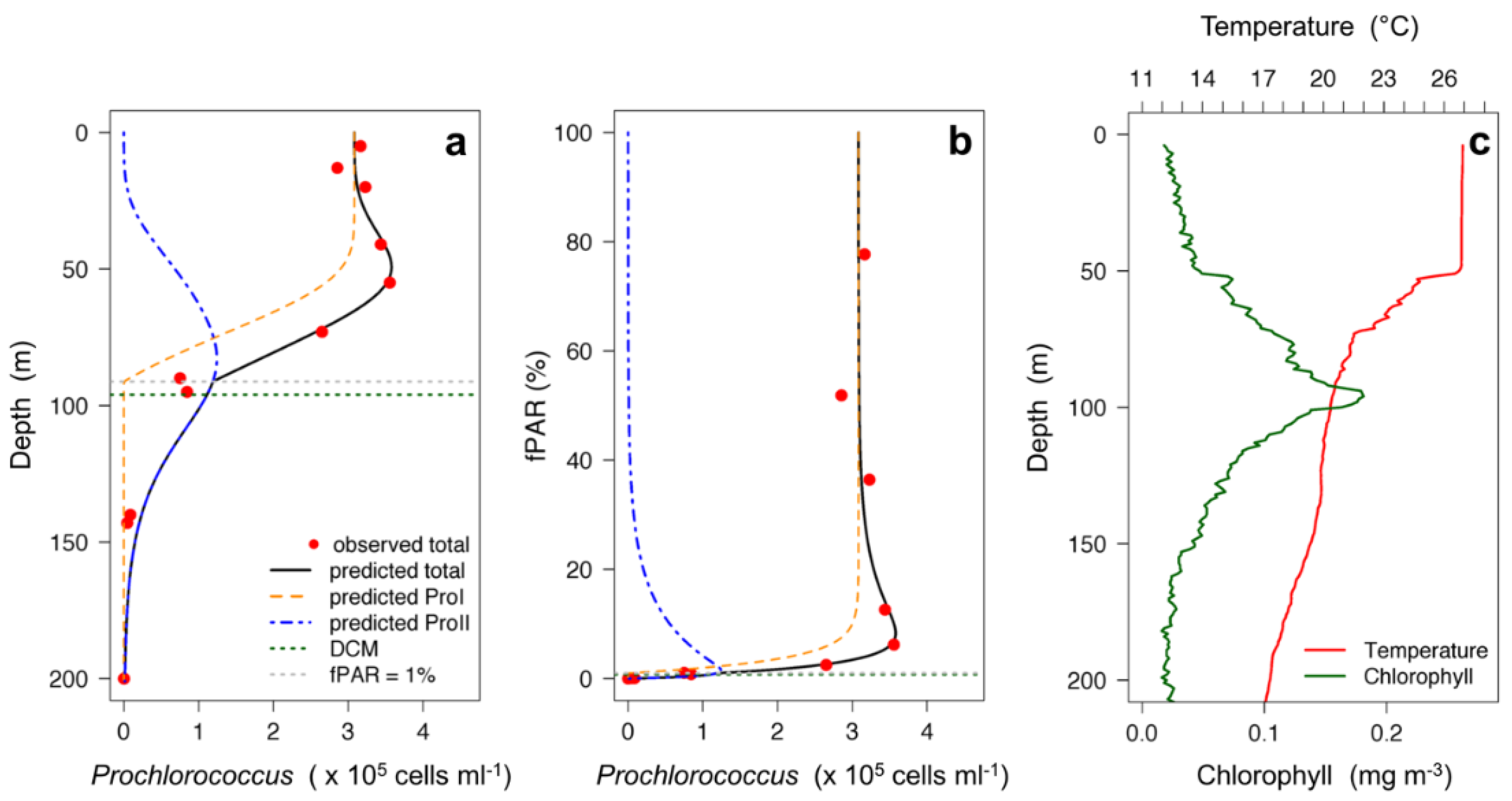
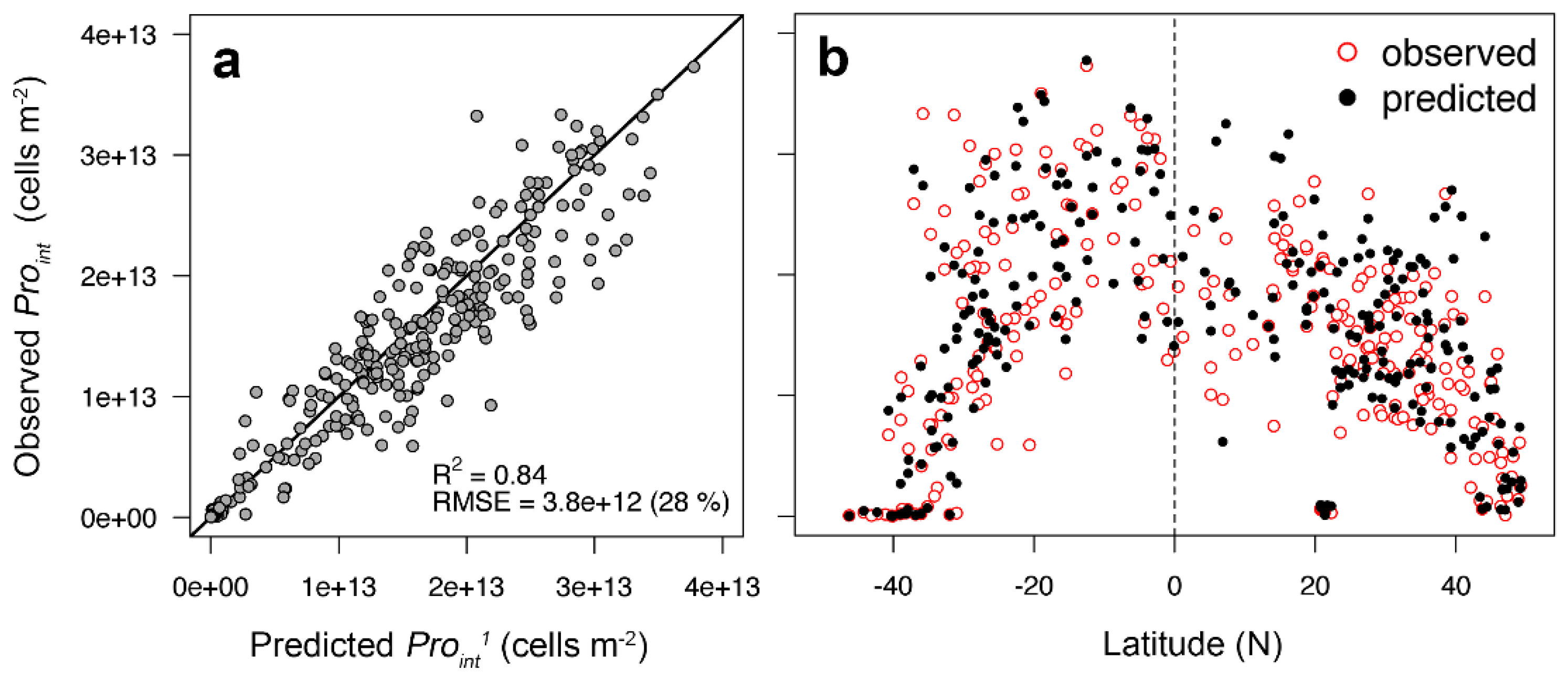
3.1. Two-Component Model Validation

The derived parameters of the model (ZDCM, KdPAR, Prosurf, Promax) that describe the shape of the abundance profile and the final products Prototal(z) and Proint were validated using 13 AMT cruises, which cover a broad swath of the Atlantic basin, and data from BATS (Bermuda Atlantic Time-Series Study).
Model estimates were compared with in situ observations using the approach proposed by Brewin et al. (2015) [31], which includes four statistical metrics: root mean square error (Ψ); average bias (δ); centre-pattern (or unbiased) root mean square error (∆); and the adjusted coefficient of determination (r2). For this, we assumed variables present a normal frequency distribution in the natural environment. Results of the statistical tests are summarised in Table 3.
When using in situ observations of the derived parameters as inputs for the model, particularly Prosurf and ZDCM (in which case Equations (1), (3)–(5) and (10) are excluded), our model robustly predicts the vertical distribution of Prochlorococcus cells in the water column (i.e., Prototal(z)1, r2 = 0.84, Figure 5b) and, consequently, produces reasonable estimates of cell concentrations integrated in the top 200 m of the water column (i.e., Proint1, r2 = 0.85, Figure 6). However, when using remotely-sensed environmental variables as inputs to estimate the derived parameters (full model from remote-sensing data), the predictive skill of the model to Prototal(z) and Proint decreases to r2 = 0.58 and r2 = 0.48, respectively (Table 3; Figure 5c and Figure 7a,b ). This increase in error is primarily caused by the difficulty in estimating Prosurf from satellite (r2 = 0.50 Figure 7c,d and Figure S9b). The reduction in performance may also be attributed to the nature of comparing observations at vastly different spatial and temporal scales: in situ cell abundance counts were taken in a few millilitres of seawater at a determined time point where environmental conditions can change in hours or days, whereas satellite data were extracted from 8-day composites and pixels cover an area of 16 km2 and Argo data were extracted from a climatology (monthly average over 6 years). Overall, the satellite-derived model is negatively biased (δ = −0.572 × 10¹² cells cm−2), and tends to underestimate cell concentrations at most depths (Figure 5c). However, the spatial variability of integrated cell abundance is still well represented (Figure 7b).

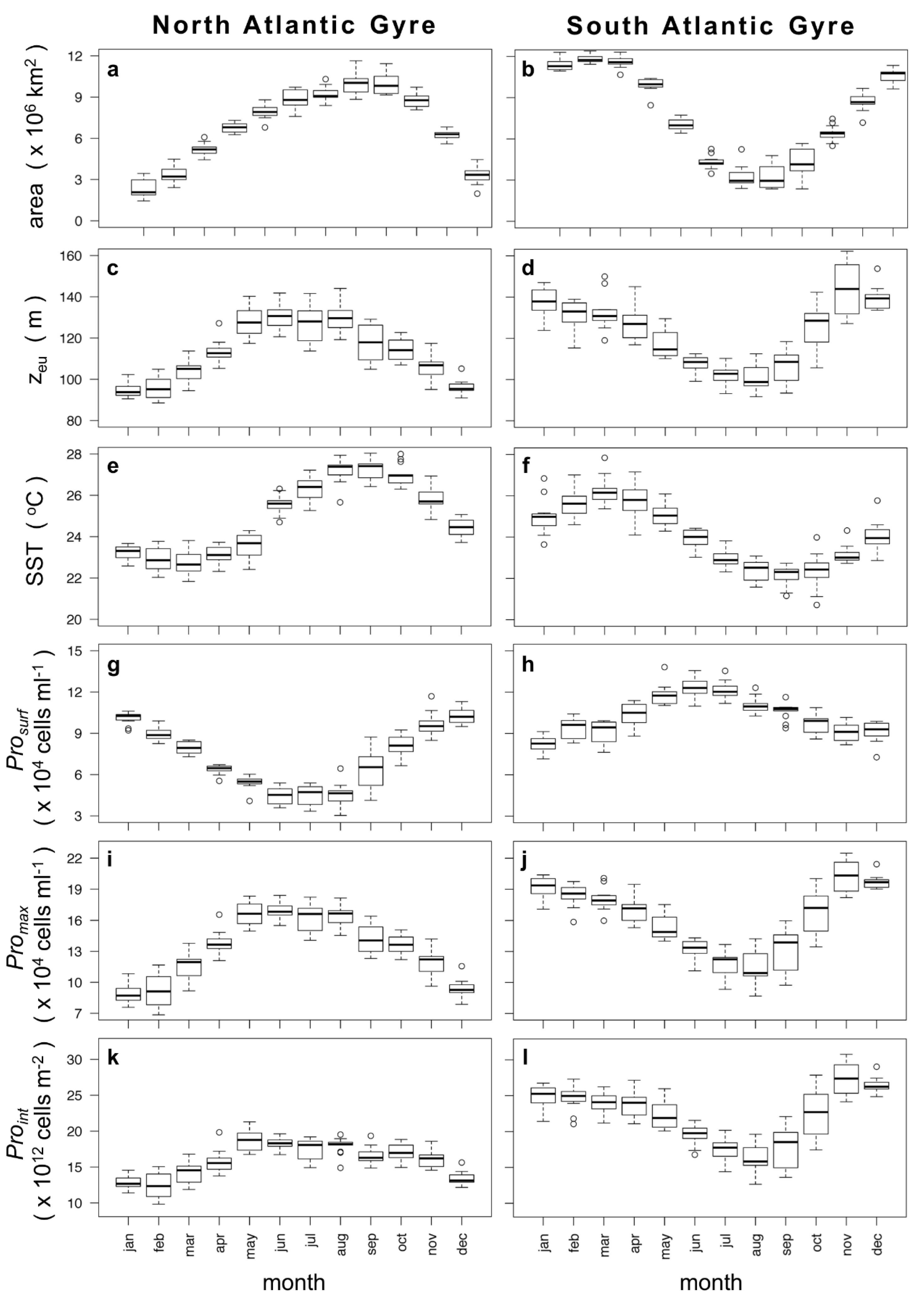
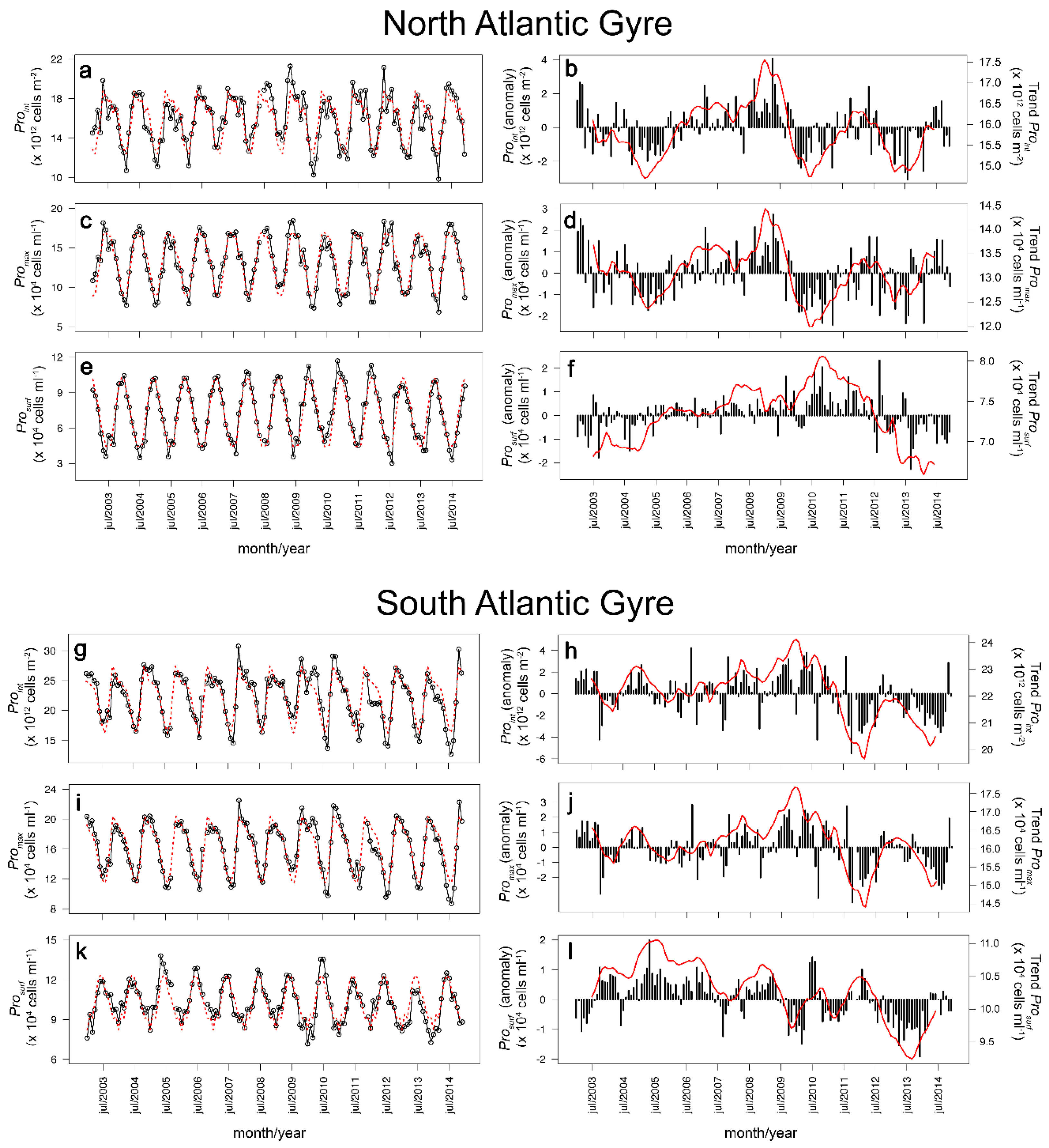
3.2. Two-Component Model Output

In the present work, we opt for using a two-component model (ProI + ProII) that is able to determine the maximum abundance of Prochlorococcus cells when it occurs at depth (Figure S7). The relevance of this deep component ProII to determine the vertical distribution of Prochlorococcus cells was tested by comparing two-component model output with a model that has only the component ProI. Details of this comparison are described in the Suppl. Material.
According to estimates of the two-component model, the Atlantic basin hosts 7.4 × 1026 Prochlorococcus cells (32 Mt of carbon, assuming an intracellular carbon concentration of 50 fg C cell−1 [19]), concentrated mainly in warm stratified waters. When combined, subtropical gyres hold the largest cell concentrations (35%), followed by the area near the Equatorial Convergence Zone (ECZ) which carries 30% of the Atlantic cell stock (Table 4, Figure 8). The total standing stock in the two Atlantic subtropical gyres varies according to both their areal extent, which expands and contracts seasonally (Figure 8 and Figure 9a,b), and to their euphotic depth (Figure 9c,d), which governs the vertical distribution of cells and the depth range over which they occur. Subtropical gyres were determined as areas where the concentration of chlorophyll at the sea surface is lower than or equal to 0.075 mg m−3 [35](more information in the Suppl. Material).
To better visualise the seasonal dynamics of these two factors controlling the standing stock of Prochlorococcus, we assessed both of these ocean properties for the North and South Atlantic Gyres, hitherto referred to as the NAG and the SAG. In their respective summer months, both the northern and southern gyres expand (Figure 9a,b) as the sea surface temperature (Figure 9e,f) and the intensity of the incident irradiance (PAR) increase [7]. The increase in these two factors foster stratification of the water column that both reduces the supply of nutrients from depth and increases the average light intensity to which phytoplankton cells are exposed [9]. The high incident irradiance leads to a reduction in the concentration of Prochlorococcus cells at surface (Prosurf) (Figure 9g,h), but since the light penetrates deeper in the water column, the growth of Prochlorococcus cells close to the DCM (Promax) is enhanced and higher concentrations are found at the DCM than at the sea surface (Figure 9i,j). Thus, the vertical profiles of cell abundance vary over the annual cycle, with Promax reaching highest concentrations from spring to autumn (Figure 8 and Figure 9i,j), whereas Prosurf is highest during winter (Figure 8 and Figure 9g,h). The integrated cell abundance in the water column (Proint) is influenced by the depth of the euphotic layer and Promax, showing seasonal variability that resembles that of Promax and thus is inverse to Prosurf (Figure 9k,l). The resemblance between Proint and Promax was also observed in their interannual variability in both gyres (Figure 10c,d,i,j).
In general, the standing stock of Prochlorococcus cells integrated over the gyre area is 1.7 times higher in the South Atlantic Gyre (SAG) than in the North Atlantic Gyre (NAG) (Table 4), regardless of the season (Figure 9k,l). No clear long-term temporal changes of Proint and Promax were observed in either of the gyres (Figure 10a,b,g,h), although a mode shift (between positive and negative anomalies) of approximately 3–5 years was observed in the NAG (Figure 10a,b). Prosurf decreased in the SAG (Figure 10k,l), whereas in the NAG there was an increase in cell abundance from 2002 to 2011, followed by a steep decrease from 2012 to 2014 (Figure 10e,f), which could be associated with the degradation of MODIS Rrs signals that started in 2012.

4. Discussion

The two-component model successfully reproduces the vertical distribution of the cell abundance of Prochlorococcus across the Atlantic Basin, including the formation of a deep abundance maximum a few metres above the DCM (see Figure 3). When provided with in situ measurements of surface cell abundance (Prosurf), the model accurately predicts the vertical distribution of cells (r2 = 0.83, see Table 3), regardless of the geographic location, showing that physical and biological processes that take place in surface layers of the water column are tightly coupled to those that occur at depth. However, when satellite data are used to determine Prosurf, model estimates of the integrated cell abundance in the water column (Proint) are more precise in the Atlantic Ocean than in other ocean basins (see Table 3), as the empirical relationships used in this algorithm were derived from data collected in the Atlantic.
Despite having roughly similar global estimates, the predicted global distribution patterns of Prochlorococcus cells are markedly different from previous studies, with our model showing higher surface cell concentrations in the area near the Equatorial Convergence Zone (ECZ) and on the periphery of subtropical gyres, and lower surface cell abundance in the core of the gyres. This distribution pattern is supported by in situ observations made in several transect cruises across the Atlantic Ocean [13,16] (see Figure 7d). Conversely, surface distributions of Prochlorococcus presented by Flombaum et al. (2013) [20] show higher cell concentrations not only in the ECZ, but also in the western sector of the ocean basins (which includes the central portion of the subtropical gyres) due to the strong relationship between Prochlorococcus cell abundance and water temperature, especially if observations at depth are taken into account.
Similar to the present study, Flombaum et al. (2013) [20] used a series of empirical equations that relate Prochlorococcus cell concentrations at the surface and at depth to the vertical structure in temperature and daily PAR. Thus, their model assumes that the same environmental factors that influence cell abundance at the surface also govern the variability in cell concentrations at depth. In the present model, the surface distribution of cells is primarily influenced by environmental conditions at the sea surface (except the variable T200 which is used as a proxy for stratification and hence nutrient input from depth). To estimate cell abundance at depth, we include an additional parameter: the maximum cell abundance at depth (Promax). The analysis of in situ data shows that the profile of Prochlorococcus is directly influenced by Promax, which in turn is related to the water-leaving radiance at 443 nm (Rrs(443)). Thus, Promax is highest when Rrs(443) is highest (i.e., in optically clear waters, there is less phytoplankton pigment at the surface, therefore less light absorption, leading to an increase in water-leaving irradiance at blue wavelengths). Conversely, cell concentrations at the surface are inversely related to Rrs(443) where sea surface temperatures are high (see coefficient e3 in Table 2), which occurs in the interior of subtropical gyres. Partitioning our Prochlorococcus population into two components (ProI near the surface and ProII at depth) allowed us to include the deep peak in Prochlorococcus cell abundance that is routinely observed in subtropical waters [13,15,16,36] and which contributes significantly to the vertically integrated cell abundance, especially in periods when surface irradiance (PAR) is high or increasing over time (i.e., summer, spring). This deep abundance maximum is neglected in the previous models, which may explain why global cell stock in Flombaum et al. (2013) [20] is lower than that estimated in the present study. Additionally, instead of using PAR, our model uses fPAR to determine the vertical distribution of cells. The reason for using a relative rather than absolute value of irradiance is because the shape of phytoplankton pigment and the abundance and productivity profiles in open ocean waters have been shown to follow changes in light attenuation rather than fluctuations in instantaneous light [37,38]. This happens possibly because PAR varies over a timescale of hours, whereas fPAR reflects a longer-term (days or weeks) change in the availability of light at depth and how the microbial community (including phytoplanktonic pigmented cells) responds to these variations over longer time periods.
As a consequence of the differences in approach between the present study and those of Flombaum et al. (2013) [20], the seasonality and temporal variability of the global Prochlocococcus cell stock are markedly different between the two models. Our results show that global and regional cell stocks of Prochlorococcus are relatively constant over time, not showing any discernible long-term trend over the 12-year study period (2003–2014). This is in part due to the areal extent of the gyres being relatively uniform from 2003 to 2014 (if seasonal oscillations are discarded), when estimated on the basis of satellite observations of chlorophyll concentration at the sea surface [7]. This result is also consistent with the view that the Prochlorococcus population consists of a “federation” of physiologically diverse cells that exhibits dynamic stability [34].
Our model detected a positive–negative anomaly cycle of 3–5 years, similar to that observed between 1991 and 2004 in the North Pacific Gyre near Hawaii (HOT time series) [15]. This cyclical oscillation may be associated with changes at depth, such as variations in the volume and/or vertical oscillations of subtropical mode waters (STMW). The STMW are voluminous subsurface (depths between ~150 and ~400 to 600 m in the Atlantic gyres) water masses located in the subtropical gyres, characterised by unique high temperature and salinity conditions that make this water mass vertically homogeneous [39]. Therefore, in subtropical gyres, oscillations in the STMW directly influence nutrient supply from depth to surface and, consequently, phytoplankton growth, including the growth of Prochlorococcus.
Water-column stability also varies seasonally, resulting in marked seasonal changes in the concentrations of Prochlorococcus cells. As ~57% of the global ocean’s area is located in the Southern Hemisphere [40], of which the occupation of subtropical gyres is greater than in the Northern Hemisphere (i.e., Figure 9a,b), the seasonal variability observed in the global Prochlorococcus cell stock (see Figure S6a) is mostly influenced by a combination of environmental conditions in the Southern Hemisphere, such as the areal extent of the Southern Subtropical Gyres (see Figure 9b), underwater light conditions, and vertical structure of the water column. As solar radiation levels increase during the summer, the gyres expand reaching the maximal extent, and the water column becomes warmer and more stratified in the gyre’s interior. This leads to extreme high-light and low-nutrient conditions that reduce the growth of phytoplankton at the surface [5]. High light levels at the sea surface also result in a reduction in the intracellular concentration of photosynthetic pigments as a consequence of phytoplankton photoacclimation [5], which is another factor leading to lower surface concentrations of chlorophyll at the sea surface in the summer [41].
The increased surface irradiance and reduced phytoplankton pigment concentration at the surface allow solar irradiance to penetrate deeper within the water column, and the lower intracellular pigment concentrations induced by higher irradiance lead to a decrease in KdPAR and a consequent increase in the limits of the euphotic zone (see Figure 9c,d). Therefore, the depth range over which Prochlorococcus has enough light to achieve net growth extends deeper, resulting in higher integrated cell abundances during the summer (see Figure 9k,l). In contrast, during the winter, lower surface irradiances and increased mixing in the water column are accompanied by an increase in cellular chlorophyll concentrations at the sea surface, leading to the contraction of the gyre’s extension [41,42]. Previous assessments of seasonal variations in Prochlorococcus populations based on in situ observations show that, in the Atlantic subtropical gyres, standing stocks of Prochlorococcus are larger during spring when compared with autumn [16]. Conversely, at the periphery of the North Atlantic gyre, Prochlorococcus is most abundant during summer and autumn [14,43]. In the North Pacific Gyre (HOT station), Rabouille et al. (2007) [15] and Malmstrom et al. (2010) [14] reported no significant seasonal changes in the integrated abundance of Prochlorococcus in the euphotic layer, but a noticeable seasonal shift in their vertical distribution was observed.
Differences between Prochlorococcus cell stocks in the NAG and the SAG may be a consequence of physical processes that govern nutrient delivery in the gyres: the degree of water column stratification and the proximity of the STMW to the bottom of the photic zone. In the SAG, the water column is strongly stratified at the bottom of the mixed layer, and a shallow pycnocline is formed during spring when surface waters start to warm. The deep thermocline occurs at 80–120 m and coincides with the nutricline; above this depth horizon the water column is relatively homogeneous (see Figure S7i). However, the amount of total kinetic energy input at the surface is low, leading to low mixing [44] within the surface ocean. The higher concentration of Prochlorococcus cells (Proint = 2.2 × 10¹³ cells m−2) in the SAG when compared with the NAG may be a consequence of either a thinner underlying STMW in the SAG or the unique vertical structure of density of this STMW [39] that may influence nutrient input from depth to the euphotic layer. Conversely, the NAG has the thickest STMW in the global ocean, and the temperature at 200 m is considerably warmer (see Figure S7f) than that found in the SAG, the ECZ, or even the NAG periphery (see Figure S7c). The lower stratification combined with higher temperatures at depths between 100 and 200 m indicates an even deeper thermocline and nutricline, leading to a lower nutrient flux from depth and thereby resulting in the lower Prochlorococcus cell stocks in the NAG (Proint = 1.6 × 10¹³ cells m−2).
Prochlorococcus numerically dominates vast expanses of the warm and strongly-stratified open ocean [13,15,34,45,46]. The sensitivity of the Prochlorococcus population as a whole to changes in physical forcing [12], such as decreased kinetic energy input to the water column, resulting in low turbulent mixing [44] and long-period internal oscillations in subsurface water masses that can lead to changes in nutrient supply from depth [39], makes this genus an ideal indicator of water-column dynamics. The preferred habitat of Prochlorococcus, the ocean’s subtropical gyres, expands and contracts according to seasonal changes in stratification, leading to significant spatiotemporal changes in the standing stocks of Prochlorococcus cells. Additionally, variations in Prochlorococcus cell stocks are a consequence of the collective physiological response of this genetically diverse assemblage of cells to both abiotic (temperature, nutrients), and biotic factors (grazing pressure, viral infection, sinking), the latter of which were not explored in the present work. Nevertheless, our model is able to recreate the basin-scale patterns in the vertical distribution of Prochlorococcus cells, which is a crucial first step to quantify the role of this globally important cyanobacterium in marine biogeochemical cycles.

5. Conclusions

Despite their minute size and cellular biomass [47], Prochlorococcus represents a significant amount of global carbon biomass: 171 Mt C contained in ~3.4 × 1027 cells. Most of this biomass is concentrated in areas near the Equatorial Convergence Zone and in the subtropical gyres. In the Atlantic, no significant temporal change was observed over the period of 2003–2014, but marked seasonal variations in cell abundance occur inside the subtropical gyres, where cell abundances are highest in the spring and summer and lowest during the winter. Although the global estimate presented here is similar to that calculated in a previous model [20], the spatial and temporal patterns in the abundance of Prochlorococcus cells differ. Our results are in agreement with observations made in the natural environment [13,15,16,36] and provide an unprecedented three-dimensional view of the distribution of Prochlorococcus biomass in the Atlantic ocean using remote-sensing observations.
This depth-resolved empirical model helps advance our ability to examine temporal changes in the biomass of Prochlorococcus over basin scales. Although the model captures the light dependence of Prochlorococcus abundance, there is scope for further refinements. The parameterisation of the model is based on a dataset that is geographically biased to the Atlantic basin, whereas data from the Pacific and Indian Oceans (PANGAEA dataset after 2002) were used only for validation (see Suppl. Material). A broader coverage of spatial in situ data can improve the equation used to estimate the abundance of Prochlorococcus cells at the sea surface (Prosurf) by regionally tuning it for each ocean basin. Improvement of estimates of Prosurf will increase the model’s ability to accurately predict of the vertical distribution of Prochlorococcus cells in other ocean basins.

Supplementary Materials

Additional information to this manuscript is available online at www.mdpi.com/2072-4292/10/6/847/S1.

Author Contributions

All authors contributed to the elaboration (writing) of this manuscript. Additionally, P.K.L., H.A.B., R.J.W.B. and S.S. conceived the model, G.A.T. and M.Z. provided flow cytometric data acquired on the cruises AMT 12 to 21, and G.D. provided and processed the Argo dataset.

Acknowledgments

This work was supported by the Atlantic Meridional Transect Program (AMT) and the Brazilian National Council for Scientific and Technological Development (CNPq) (PhD GDE scholarship 211546/2013-5). The AMT dataset is supported by the UK Natural Environment Research Council National Capability funding to Plymouth Marine Laboratory and the National Oceanography Centre, Southampton. The authors would like to thank the British Oceanographic Data Centre (BODC), and the International Argo Program and national programs that contribute to it (http://www.argo.ucsd.edu, http://argo.jcommops.org) for providing the datasets used in this manuscript. The authors also thank the Ocean Biology Processing Group of NASA for the processing and distribution of MODIS-Aqua data used in this manuscript.

Conflicts of Interest

The authors declare no conflict of interest.

References

  1. Hirata, T.; Aiken, J.; Hardman-mountford, N.; Smyth, T.J.; Barlow, R.G. Remote Sensing of Environment an absorption model to determine phytoplankton size classes from satellite ocean colour. Remote Sens. Environ. 2008, 112, 3153–3159. [Google Scholar] [CrossRef]
  2. Karl, D.M. Minireviews: A Sea of Change: Biogeochemical Variability in the North Pacific Subtropical Gyre. Ecosystems 1999, 2, 181–214. [Google Scholar] [CrossRef]
  3. Longhurst, A. Ecological Geography of the Sea; Academic Press: San Diego, CA, USA, 1998. [Google Scholar]
  4. Olson, D.M.; Dinerstein, E.; Wikramanayake, E.D.; Burgess, N.D.; Powell, G.V.N.; Underwood, E.C.; D’amico, J.A.; Itoua, I.; Strand, H.E.; Morrison, J.C.; et al. Terrestrial Ecoregions of the World: A New Map of Life on Earth. Bioscience 2001, 51, 933–938. [Google Scholar] [CrossRef]
  5. Behrenfeld, M.J.; O’Malley, R.T.; Boss, E.S.; Westberry, T.K.; Graff, J.R.; Halsey, K.H.; Milligan, A.J.; Siegel, D.A.; Brown, M.B. Revaluating ocean warming impacts on global phytoplankton. Nat. Clim. Chang. 2015, 6, 323–330. [Google Scholar] [CrossRef]
  6. Westberry, T.; Behrenfeld, M.J.; Siegel, D.A.; Boss, E. Carbon-based primary productivity modeling with vertically resolved photoacclimation. Glob. Biogeochem. Cycles 2008, 22. [Google Scholar] [CrossRef]
  7. Aiken, J.; Brewin, R.J.W.; Dufois, F.; Polimene, L.; Hardman-Mountford, N.J.; Jackson, T.; Loveday, B.; Hoya, S.M.; Dall’Olmo, G.; Stephens, J.; et al. A synthesis of the environmental response of the North and South Atlantic Sub-Tropical Gyres during two decades of AMT. Prog. Oceanogr. 2016. [Google Scholar] [CrossRef]
  8. Cullen, J.J. The deep chlorophyll maximum: Comparing vertical profiles of chlorophyll a. Can. J. Fish. Aquat. Sci. 1982, 39, 791–803. [Google Scholar] [CrossRef]
  9. Kirk, J.T.O. Light and Photosynthesis in Aquatic Ecosystems, 3rd ed.; Cambridge University Press: Cambridge, UK, 2011; ISBN 978-0-521-15175-7. [Google Scholar]
  10. Grace, J.; San Jose, J.; Meir, P.; Miranda, H.S.; Montes, R.A. Productivity and carbon fluxes of tropical savannas. J. Biogeogr. 2006, 33, 387–400. [Google Scholar] [CrossRef]
  11. Chisholm, S.W.; Olson, R.J.; Zettler, E.R.; Goericke, R.; Waterbury, J.B. A novel free-living prochlorophyte abundant in the oceanic euphotic zone. Nature 1988, 334, 340–343. [Google Scholar] [CrossRef]
  12. Bouman, H.A.; Ulloa, O.; Barlow, R.; Li, W.K.W.; Platt, T.; Zwirglmaier, K.; Scanlan, D.J.; Sathyendranath, S. Water-column stratification governs the community structure of subtropical marine picophytoplankton. Environ. Microbiol. Rep. 2011, 3, 473–482. [Google Scholar] [CrossRef] [PubMed]
  13. Heywood, J.L.; Zubkov, M.V.; Tarran, G.A.; Fuchs, B.M.; Holligan, P.M. Prokaryoplankton standing stocks in oligotrophic gyre and equatorial provinces of the Atlantic Ocean: Evaluation of inter-annual variability. Deep Sea Res. II Top. Stud. Oceanogr. 2006, 53, 1530–1547. [Google Scholar] [CrossRef]
  14. Malmstrom, R.R.; Coe, A.; Kettler, G.C.; Martiny, A.C.; Frias-Lopez, J.; Zinser, E.R.; Chisholm, S.W. Temporal dynamics of Prochlorococcus ecotypes in the Atlantic and Pacific oceans. ISME J. 2010, 4, 1252–1264. [Google Scholar] [CrossRef] [PubMed] [Green Version]
  15. Rabouille, S.; Edwards, C.A.; Zehr, J.P. Modelling the vertical distribution of Prochlorococcus and Synechococcus in the North Pacific Subtropical Ocean. Environ. Microbiol. 2007, 9, 2588–2602. [Google Scholar] [CrossRef] [PubMed]
  16. Zubkov, M.V.; Sleigh, M.A.; Burkill, P.H.; Leakey, R.J.G. Picoplankton community structure on the Atlantic Meridional Transect: A comparison between seasons. Prog. Oceanogr. 2000, 45, 369–386. [Google Scholar] [CrossRef]
  17. Zubkov, M.V.; Sleigh, M.A.; Tarran, G.A.; Burkill, P.H.; Leakey, R.J.G. Picoplanktonic community structure on an Atlantic transect from 50 degrees N to 50 degrees S. Deep Sea Res. I Oceanogr. Res. Pap. 1998, 45, 1339–1355. [Google Scholar] [CrossRef]
  18. Smayda, T.J. Bloom dynamics: Physiology, behavior, trophice: Ffects. Limonaology Oceanogr. 1997, 42, 1132–1136. [Google Scholar] [CrossRef]
  19. Bertilsson, S.; Berglund, O.; Karl, D.M.; Chisholm, S.W. Elemental composition of marine Prochlorococcus and Synechococcus: Implications for the ecological stoichiometry of the sea. Limnol. Oceanogr. 2003, 48, 1721–1731. [Google Scholar] [CrossRef]
  20. Flombaum, P.; Gallegos, J.L.; Gordillo, R.A.; Rincon, J.; Zabala, L.L.; Jiao, N.; Karl, D.M.; Li, W.K.W.; Lomas, M.W.; Veneziano, D.; et al. Present and future global distributions of the marine Cyanobacteria Prochlorococcus and Synechococcus. Proc. Natl. Acad. Sci. USA 2013, 110, 9824–9829. [Google Scholar] [CrossRef] [PubMed]
  21. Williams, R.G.; Follows, M.J. Biological Fundamentals. In Ocean Dynamics and the Carbon Cycle: Principles and Mechanisms; Williams, R.G., Follows, M.J., Eds.; Cambridge University Press: New York, NY, USA, 2011. [Google Scholar]
  22. NASA Moderate Resolution Imaging Spectroradiometer (MODIS-Aqua) Ocean Color Data; Goddard Space Flight Center Ocean Biology Processing Group: Greenbelt, MD, USA, 2014.
  23. Gordon, H.R.; Morel, A.Y. Remote Assessment of Ocean Color for Interpretation of Satellite Visible Imagery; Springer-Verlag New York: New York, USA, 1983. [Google Scholar]
  24. Hosoda, S.; Ohira, T.; Nakamura, T. A monthly mean dataset of global oceanic temperature and salinity derived from Argo float observations. JAMSTEC Rep. Res. Dev. 2008, 8, 47–59. [Google Scholar] [CrossRef]
  25. Johnson, Z.I.; Zinser, E.R.; Coe, A.; McNulty, N.P.; Woodward, E.M.; Chisholm, S.W. Niche Partitioning Among Prochlorococcus Ecotypes Along Ocean-Scale Environmental Gradients. Science 2006, 311, 1737–1740. [Google Scholar] [CrossRef] [PubMed]
  26. Zinser, E.R.; Johnson, Z.I.; Coe, A.; Karaca, E.; Veneziano, D.; Chisholm, S.W. Influence of light and temperature on Prochlorococcus ecotype distributions in the Atlantic Ocean. Limnol. Oceanogr. 2007, 52, 2205–2220. [Google Scholar] [CrossRef]
  27. Platt, T.; Gallegos, C.L.; Harrison, W.G. Photoinhibition of photosynthesis in natural assemblages of marine phytoplankton. J. Mar. Res. 1980, 38, 687–701. [Google Scholar]
  28. De Boyer Montégut, C.; Madec, G.; Fischer, A.S.; Lazar, A.; Iudicone, D. Mixed layer depth over the global ocean: An examination of profile data and a profile-based climatology. J. Geophys. Res. Oceans 2004, 109, 1–20. [Google Scholar] [CrossRef]
  29. Morel, A.; Berthon, J.-F. Surface pigments, algal biomass profiles, and potential production of the euphotic layer: Relationships reinvestigated in view of remote-sensing applications. Limnol. Oceanogr. 1989, 34, 1545–1562. [Google Scholar] [CrossRef]
  30. Venables, W.N.; Ripley, B.D. Modern Applied Statistics with S, 4th ed.; Springer: New York, NY, USA, 2002; Volume 53, ISBN 0387954570. [Google Scholar]
  31. Brewin, R.J.W.; Sathyendranath, S.; Müller, D.; Brockmann, C.; Deschamps, P.Y.; Devred, E.; Doerffer, R.; Fomferra, N.; Franz, B.; Grant, M.; et al. The Ocean Colour Climate Change Initiative: III. A round-robin comparison on in-water bio-optical algorithms. Remote Sens. Environ. 2015, 162, 271–294. [Google Scholar] [CrossRef]
  32. Forsythe, W.C.; Rykiel, E.J.; Stahl, R.S.; Wu, H.I.; Schoolfield, R.M. A model comparison for daylength as a function of latitude and day of year. Ecol. Model. 1995, 80, 87–95. [Google Scholar] [CrossRef]
  33. Cooper, P.I. The absorption of radiation in solar stills. Sol. Energy 1969, 12, 333–346. [Google Scholar] [CrossRef]
  34. Biller, S.J.; Berube, P.M.; Lindell, D.; Chisholm, S.W. Prochlorococcus: The structure and function of collective diversity. Nat. Rev. Microbiol. 2014, 13, 13–27. [Google Scholar] [CrossRef] [PubMed]
  35. McClain, C.R.; Signorini, S.R.; Christian, J.R. Subtropical gyre variability observed by ocean-color satellites. Deep Sea Res. II Top. Stud. Oceanogr. 2004, 51, 281–301. [Google Scholar] [CrossRef]
  36. Brew, H.S.; Moran, S.B.; Lomas, M.W.; Burd, A.B. Plankton community composition, organic carbon and thorium-234 particle size distributions, and particle export in the Sargasso Sea. J. Mar. Res. 2009, 67, 845–868. [Google Scholar] [CrossRef]
  37. Behrenfeld, M.J.; Falkowski, P.G. Photosynthetic rates derived from satellite-based chlorophyll concentration. Limnol. Oceanogr. 1997, 42, 1–20. [Google Scholar] [CrossRef]
  38. Babin, M.; Therriault, J.C.; Legendre, L.; Nieke, B.; Reuter, R.; Condal, A. Relationship between the maximum quantum yield of carbon fixation and the minimum quantum yield of chlorophyll a in vivo fluorescence in the Gulf of St. Lawrence. Limnol. Oceanogr. 1995, 40, 956–968. [Google Scholar] [CrossRef]
  39. Tsubouchi, T.; Suga, T.; Hanawa, K. Comparison study of subtropical mode waters in the world ocean. Front. Mar. Sci. 2016, 3, 270. [Google Scholar] [CrossRef]
  40. Boggs, S.W. This Hemisphere. J. Geol. 1945, 44, 345–355. [Google Scholar] [CrossRef]
  41. Dave, A.C.; Barton, A.D.; Lozier, M.S.; McKinley, G.A. What drives seasonal change in oligotrophic area in the subtropical North Atlantic? J. Geophys. Res. Oceans 2015, 120, 3958–3969. [Google Scholar] [CrossRef]
  42. Polovina, J.J.; Howell, E.A.; Abecassis, M. Ocean’s least productive waters are expanding. Geophys. Res. Lett. 2008, 35, L03618. [Google Scholar] [CrossRef]
  43. Durand, M.D.; Olson, R.J.; Chisholm, S.W. Phytoplankton population dynamics at the Bermuda Atlantic Time-series station in the Sargasso Sea. Deep Sea Res. II Top. Stud. Oceanogr. 2001, 48, 1983–2003. [Google Scholar] [CrossRef]
  44. Barton, A.D.; Ward, B.A.; Williams, R.G.; Follows, M.J. The impact of fine-scale turbulence on phytoplankton community structure. Limnol. Oceanogr. Fluids Environ. 2014, 4, 34–49. [Google Scholar] [CrossRef]
  45. Buitenhuis, E.T.; Li, W.K.W.; Vaulot, D.; Lomas, M.W.; Landry, M.R.; Partensky, F.; Karl, D.M.; Ulloa, O.; Campbell, L.; Jacquet, S.; et al. Picophytoplankton biomass distribution in the global ocean. Earth Syst. Sci. Data 2012, 4, 37–46. [Google Scholar] [CrossRef] [Green Version]
  46. Mella-Flores, D.; Six, C.; Ratin, M.; Partensky, F.; Boutte, C.; Le Corguillé, G.; Marie, D.; Blot, N.; Gourvil, P.; Kolowrat, C.; Garczarek, L. Prochlorococcus and synechococcus have evolved different adaptive mechanisms to cope with light and uv stress. Front. Microbiol. 2012, 3, 285. [Google Scholar] [CrossRef] [PubMed] [Green Version]
  47. Partensky, F.; Hess, W.R.; Vaulot, D. Prochlorococcus, a marine photosynthetic prokaryote of global significance. Microbiol. Mol. Biol. Rev. 1999, 63, 106–127. [Google Scholar] [PubMed]
Figure 1. Transects of the 13 AMT cruises (704 stations) used to create the empirical model to predict the abundance of Prochlorococcus cells.
Remotesensing 10 00847 g001
Figure 2. Flowchart of computations used to calculate the cell abundance of Prochlorococcus. Variable acronyms and symbols are described in Table 1.
Remotesensing 10 00847 g002
Figure 3. Vertical profiles of observed and estimated Prochlorococcus cell abundances (a) over depth and (b) over the fractional PAR fPAR, with (c) corresponding profiles of temperature and chlorophyll from CTD measurements at a site inside the North Atlantic Gyre (26° N, 50° W). For (a,b), in situ observations are represented by red dots, predicted profiles of ProI by the orange dashed line, predicted profiles of ProII by the blue dashed line, and predicted profiles of total Prochlorococcus abundance by the solid black line. Data from AMT 24 (2014).
Remotesensing 10 00847 g003
Figure 4. (a) Comparison between observed versus predicted depth of the deep chlorophyll maximum (ZDCM) across the Atlantic Ocean (locations displayed in Figure 1) using Equation (8) of the present work; (b) Observed (AMT12-24, n = 693 observations) and predicted ZDCM (n = 449) in the Atlantic Ocean (AMTs 12 to 24, locations displayed in Figure 1). For each CTD cast, observed ZDCM was determined as the depth of the maximum chlorophyll concentration measured using the CTD fluorometer.
Remotesensing 10 00847 g004
Figure 5. Vertical profiles of Prochlorococcus cell abundance over depth (Prototal(z)) across the Atlantic Ocean (locations displayed in Figure 1): (a) observed in situ on AMTs 12–24 (Prototal(z) ); (b) predicted using the partial model with observed inputs of Prosurf and ZDCM (Prototal(z)1 from Equations (1) to (2) and (6) to (7)); and (c) predicted using the full model with remote-sensing inputs (Prototal(z)3 from Equations (1)–(9).
Remotesensing 10 00847 g005
Figure 6. (a) Comparison between observed and predicted Prochlorococcus cell abundance integrated in the water column (Proint1) across the Atlantic Ocean (locations displayed in Figure 1) using the partial model where in situ observations of ZDCM, KdPAR, and Prosurf are used as inputs (i.e., Equations (1), (3)–(5), and (8) are excluded); (b) Observed and predicted Proint1 across the Atlantic Ocean (AMTs 12–24).
Remotesensing 10 00847 g006
Figure 7. (a) Comparison between observed and predicted Prochlorococcus cell abundance integrated in the water column (Proint3) across the Atlantic Ocean (locations displayed in Figure 1) using the complete model (Equations (1)–(10) of the present work); (b) Observed and predicted Proint3 across the Atlantic Ocean (AMTs 12–24); (c) Comparison between observed and predicted Prochlorococcus cell abundance at the sea surface (Prosurf) using Equations (3)–(5) of the present work; (d) Observed and predicted Prosurf across the Atlantic Ocean (AMTs 12–24).
Remotesensing 10 00847 g007
Figure 8. Estimated monthly distribution of the Prochlorococcus cells integrated in the top 200 m of the water column (Proint) (cells m−2), with correspondent vertical profiles of estimated Prochlorococcus cell abundance (cells l−1) at sites (white dots) in the North Atlantic Gyre (NAG) and South Atlantic Gyre: ProI(z) is indicated by the orange dashed line, ProII(z) by the blue dashed line, and the total Prochlorococcus abundance by the solid black line. Cell abundance was calculated based on the monthly climatology of environmental variables [22].
Remotesensing 10 00847 g008
Figure 9. Monthly averages of (a) the areal extent of the North Atlantic Gyre (NAG) and (b) South Atlantic Gyre (SAG); (c) the euphotic depth zeu at the NAG and (d) the SAG; (e) sea surface temperature SST at the NAG and (f) the SAG; (g) the estimated Prochlorococcus cell abundance at the sea surface (Prosurf) at the NAG and (h) the SAG; (i) Prochlorococcus cell abundance at the deep maximum (Promax) at the NAG and (j) the SAG; and (k) Prochlorococcus cell abundance integrated in the water column (Proint) at the NAG and (l) the SAG. Subtropical Gyres were defined as regions where the surface chlorophyll concentrations were lower than 0.075 mg m−3. The euphotic depth was estimated using the calculated KdPAR using Equation (1), and SST measurements were taken from monthly satellite composites from January 2003 to December 2014 [22]. Prochlorococcus cell abundance was computed using monthly averaged input variables for the years 2003–2014 [22], at specific locations inside the Atlantic gyres: NAG: 26° N, 50° W; SAG: 20° S, 20° W.
Remotesensing 10 00847 g009
Figure 10. Time series of (a,g) the estimated Prochlorococcus cell abundance integrated in the water column (Proint), (c,i) estimated Prochlorococcus cell abundance at the deep maximum (Promax), and (e,k) estimated Prochlorococcus cell abundance at surface (Prosurf), at one location (26° N, 50° W) in the North Atlantic Gyre (NAG) (af), and one location (20° S, 20° W) in the South Atlantic Gyre (SAG) (gl). Figures (b,d,f,h,j,l) show the time-series anomalies (black bars) and trends (red lines). Anomalies were calculated by subtracting the monthly climatology (dashed red lines in figures (a,c,e,g,i,k)) from the calculated values for each month (black lines in figures (a,c,e,g,i,k)).
Remotesensing 10 00847 g010
Table 1. List of acronyms and symbols used in this manuscript (input variables used in the predictive model of Prochlorococcus cell abundance).
SymbolVariableUnitsSource
SSTSea surface temperature°Ca
Rrs(443)Remote-sensing reflectance at 443 nmsr−1a
Rrs(488)Remote-sensing reflectance at 488 nmsr−1a
T200Temperature at the depth of 200 m°Cb
DLDay lengthhoursc
θsSolar zenith angle at noondegreesd
KdPARCalculated attenuation coefficient for the photo-synthetically available radiationm−1f
KdPAR Measured attenuation coefficient for the photo-synthetically available radiationm−1e
DCMDeep chlorophyll maximum
DPMDeep Prochlorococcus maximum
ZDCMCalculated depth of the deep chlorophyll maximummetresf
ZDCM In situ depth of the deep chlorophyll maximummetresf
fPAR(z)Fractional PAR (proportion of surface PAR) at depth z%f
ProsurfCalculated Prochlorococcus cell abundance at the surfacecells mL−1f
Prosurf In situ Prochlorococcus cell abundance at the surfacecells mL−1f
PromaxProchlorococcus cell abundance at the DPMcells mL−1f
ProICalculated cell abundance of Prochlorococcus distributed over depth near the surfacecells mL−1f
ProIICalculated cell abundance of Prochlorococcus distributed over depth near the DPMcells mL−1f
Prototal(z)Calculated total Prochlorococcus cell abundance distributed over depthcells mL−1f
ProintCalculated cell abundance of Prochlorococcus integrated in the surface 200 m of the water columncells m−2f
a. Aqua-MODIS, Ocean Color, NASA (2014) [22]; b. Argo dataset (http://argo.jcommops.org); c. Forsythe et al. (1995) [32]; d. Cooper (1969) [33]; e. Kirk (2011) [9]; f. This work.
Table 2. Parameters and coefficients used in Equations (1) to (8) with their standard deviations (σ).
OutputInput (s)EquationParameterParameter ValueParameter σ
KdPAR (1)intercept0.776 × 10−10.020 × 10⁻¹
Rrs(443)(1)slope−3.1673 × 1000.195 × 100
ZDCM (8)intercept1.241 × 1010.786 × 101
Rrs(443)(8)slope11.021 × 1040.066 × 104
θs(8)slope22.227 × 10−12.381 × 10⁻¹
ProsurfSST(3)–(5)a33.254 × 1040.030 × 104
Rrs(488)(3)–(5)b39.762 × 1070.104 × 107
DL(3)–(5)c3−2.080 × 1040.043 × 104
T200(3)–(5)d3−2.117 × 1040.029 × 104
SST, Rrs(488)(3)–(5)e3−4.421 × 1060.041 × 106
Promax (7)a7−1.153 × 1050.194 × 105
ZDCM(7)b71.837 × 1030.014 × 103
Prosurf(7)c72.951 × 10−10.087 × 10⁻¹
Table 3. Response variables with their respective root mean square error (Ψ), bias (δ), centre-root (unbiased) mean square error (∆), and determination coefficient (r2) when compared with in situ data from 13 AMT cruises. Variable definitions are listed in Table 1.
VariableEquationΨδr2
KdPAR(1)5.136 × 10⁻³−0.321 × 10−30.512 × 10−30.75
ZDCM(8)2.084 × 101−0.101 × 1012.081 × 1010.73
Promax1(7)5.872 × 10⁴−0.054 × 1045.872 × 1040.44
Prototal(z)1(9)3.775 × 10⁴−0.361 × 1043.758 × 1040.84
Proint1(10)3.682 × 10¹²−1.047 × 10123.529 × 10120.85
Promax2(7)5.805 × 10⁴−0.349 × 1045.794 × 1040.40
Prototal(z)2(9)4.038 × 10⁴−0.479 × 1044.010 × 1040.82
Proint2(10)4.146 × 10¹²−1.214 × 10123.964 × 10120.81
Prosurf3(3)–(5)6.551 × 1041.237 × 1046.434 × 1040.50
Promax3(7)6.210 × 1040.297 × 1046.203 × 1040.32
Prototal(z)3(9)6.176 × 1040.466 × 1046.159 × 1040.58
Proint3(10)6.651 × 10¹²−0.572 × 10126.651 × 10120.48
Prochlorococcus cell abundances calculated using: 1 in situ Prosurf (Prosurf) and in situ ZDCM (ZDCM); 2 in situ Prosurf and modelled ZDCM; 3 modelled Prosurf and modelled ZDCM.
Table 4. Predicted Prochlorococcus standing stock in the oceans, integrated horizontally and vertically at each area. Values were computed using Equations (1)–(10), with monthly climatology products used as input variables [22], then averaged over the year. Proint3, Prosurf3 and Promax3 were calculated at specific geographic locations within each Atlantic gyre (coordinates in the table).
Standing Stock (Cells)Total Carbon * (Megatonnes C)Proint3 (Cells m−2)Prosurf3 (Cells mL−1)Promax3 (Cells mL−1)
Global3.4 × 1027171
Atlantic Ocean7.4 × 102637
Equatorial Convergence Zone2.2 × 102611
ECZ: 2 °S, 22 °W 1.7 × 10132.2 × 1050.7 × 105
North Atlantic Gyre1.0 × 10265.1
NAG: 26° N, 50° W 1.6 × 10130.7 × 1051.3 × 105
South Atlantic Gyre1.6 × 10268.2
SAG: 20° S, 20° W 2.2 × 10131.0 × 1051.7 × 105
* using 50 fg C cell−1 to convert cell concentrations to carbon units [19].

