Operational Built-Up Areas Extraction for Cities in China Using Sentinel-1 SAR Data

Abstract

To obtain accurate information in a timely manner on built-up areas (BAs) is essential for urban planning and natural hazard (e.g., earthquakes) response strategies. In this paper, a new method for BAs extraction using the Sentinel-1 SAR is proposed, which includes two steps: (1) Candidate BAs are first selected as seeds from images that show high backscattering and obvious textural patterns, as characterized by image intensity, Getis-Ord index, and the variogram texture features; (2) region growing is iteratively implemented from these seed pixels to extract the BAs. Sentinel-1 data, with 5 × 20 m² resolution, are selected over eight cities with various environmental settings around China, to validate the robustness of the proposed method. The results show that the proposed method achieves higher detection accuracy and fewer commission errors compared with the intensity-based region growing and thresholding methods. An averaged accuracy of 96.5% in validation points of eight cities was achieved, which outperforms the GlobCover urban product in both urban and rural area, while fewer commission errors were achieved compared to Landsat data-based methods. Moreover, two polarizations (VV/VH) and the averaged channel are compared for BAs extraction in areas with various environments. It turns out that improved results can be achieved using the averaged image of two polarizations in north China, while the VV image is better suited for BAs extraction in south. These findings indicate that operational BAs mapping over China, and even globally, is possible, since the Sentinel-1 data can provide images with global coverage.

1. Introduction

It is estimated that up to 66% of the world’s population will live in urban areas by 2050. Although built-up areas occupy only a small part of global land cover, urban areas significantly alter ecological and socioeconomic environments, because cities are the main sites of traffic, production, consumption, and so on. Therefore, accurate and timely information about the spatial distribution of built-up areas is essential for urban planning, and for the creation of strategies by The Red Cross and government post-disaster teams in cities that are vulnerable to natural hazards, such as earthquake, landslides, subsidence, tsunamis, and so on.

Spaceborne earth observation using optical sensors is a valuable tool for gaining data on the characteristics and development of built-up areas [1,2,3,4,5]. Landsat and SPOT satellite images were successfully used to monitor historical land cover changes [6,7,8], and project future patterns of urban development in metropolitan regions [7]. Olivia et al. [9] used the nighttime light (NTL) data to monitor the spatial expansion of 41 urban areas in Indonesia from 1992–2012. Abass et al. [10] used Landsat images to examine land use and land cover changes, as well as the effects of peri-urbanisation on arable land. Landsat and MODIS data were also used to quantify urban sprawl and analyze its influence on net primary productivity (NPP) [11]. Nevertheless, the need for 100% cloud-free conditions, and the optimal acquisition time (in summer), limited the selection of images for the timely acquisition of land cover change information. Compared with optical sensors, synthetic aperture radar (SAR) systems can work during both day and night and under all weather conditions. This yields more reliable SAR data in perennially cloudy and rainy areas compared to optical images. A status report on the application of SAR for settlement detection, population estimation, assessment of the impact of human activities on the physical environment, mapping and analyzing urban land use patterns, and interpretation of socioeconomic characteristics has been published [12]. Indeed, SAR images—processed using appropriate elaboration algorithms—were successfully used in different fields of geosciences [13], and in particular, in recent decades, for analyzing the effects induced by many natural [14,15,16] or anthropogenic phenomena [17,18]. As for BAs extraction, although SAR data do not successfully extract information on all kinds of buildings because of the complexity of assessing built-up areas [19], advancements have been made in extracting the extent of human settlement by using single polarized, dual polarized, and full polarimetric SAR data. In terms of SAR-based BAs-extraction methods, texture measures [20], contextual information [21], local indicators of spatial association (L.I.S.A) [22], support vector machine (SVM) [23], neural network [24,25], and knowledge-based [26] approaches have been investigated with varying levels of success.

In recent years, BA extraction has been extended to the global scale. In [27], a supervised method was used to present the results of mapping the global distribution of urban land use, composed predominately of large cities at 500 m spatial resolution using remotely sensed data from the moderate-resolution imaging spectroradiometer (MODIS). Relatively accurate results were obtained, but this approach did not consider small towns and villages. The GlobCover 2009 product [28] was obtained using multispectral data from the medium-resolution imaging spectrometer (MERIS) instrument on board the Envisat-1 satellite from the European Space Agency (ESA). Pesaresi et al. [29] gave a general framework for processing high- and very high-resolution imagery in support of a Global Human Settlement Layer using the input image data, with resolution ranging from 0.5 to 10 m, collected by satellite SPOT (2 and 5), CBERS 2B, RapidEye (2 and 4), WorldView (1 and 2), GeoEye 1, QuickBird 2, Ikonos 2, and airborne sensors. Some urban extraction attempts have also been made on a global scale using SAR data. The recent release of the global urban footprint (GUF) [30] from TerraSAR-X measurements by the German Soace Afency (DLR) is paving the way for a new generation of urban remote sensing products. To evaluate ENVISAT SAR data for global urban mapping, one study [31] developed the KTH-Pavia Urban Extractor to effectively extract urban areas and small towns using ENVISAT ASAR 30 m data. While the results are very encouraging, the algorithm is time consuming when GLCM texture features are included. In another study developed by [32], a new approach based on information theory for automatic pattern recognition in earth observation (EO) big data sets was introduced, and has delivered state-of-the-art performance. Gamba and Lisini [33] developed a fast and efficient approach for global human settlement extent extraction using ENVISAT ASAR wide swath mode data with a 75 m resolution, and obtained more accurate results than the existing global data sets, including Globcover 2009. The method was successful in extracting urban areas in test areas from around the world, but the results relied on only the amplitude of the image, which may yield a precise BAs map from 75-m resolution data, but may not be entirely suitable for SAR data with moderate resolution, e.g., the data from the recently launched Sentinel-1 SAR, which have a resolution of approximately 20 m. Because the textures in BAs are more obvious in data with higher resolution than in data with a 75-m resolution, extracting BAs based only on image intensity can reduce accuracy to some extent.

To overcome this problem, in this work additional spatial index and texture features are introduced using Sentinel-1 SAR data, since it offers a good opportunity to develop a service for detecting BAs at the global scale with its freely available data, global coverage, and quick delivery. In this regard, this research aims to develop an operational and efficient procedure for Sentinel-1 SAR data to set the stage for accurate global built-up area mapping. The robustness of the proposed procedure was tested on eight cities distributed over China, including a wide variety of natural environments and building structural types. The remainder of this paper is organized as follows: Section 2 gives a description of the study areas. The proposed framework is described in Section 3. Section 4 is devoted to the experiments and a detailed analysis. Finally, the discussion and conclusions are presented in Section 5 and Section 6, respectively.

2. Study Area and Available SAR Data

The geographical environmental settings in China are complicated and building structures are various, e.g., rural settlements in the north of China are almost bungalows, and are intensively distributed, while those in southern China are small and scattered. With this in mind, eight cities in different parts of China have been selected as study areas, including cities and several small towns and villages. Among the cities, some are inland (e.g. Beijing) or coastal cities (e.g. Tianjin), and some are mountainous (e.g. Chongqing), or are surrounded by mountains (e.g., Beijing, Taiyuan and Chengdu). Three of them are municipalities (Beijing, Tianjin and Chongqing) which are under rapid urbanization, while others are all provincial capitals. Additionally, Wuhan is a city by the Yangtze River, and Hangzhou is located in China’s most developed southeastern Yangtze River Delta. For these cities, Sentinel-1 SAR images of these cities with Interferometric Wide swath (IW) mode and 5 × 20 m² resolution were acquired, whose detailed characteristics are reported in

Table 1. Sentinel-1 SAR data characteristics for study areas.

Area in PR China	City	Acquisition Date	Orbit Type	Pixel Spacing rg/az (m × m)	Incidence Angles (°)	Pol.
North	Tianjin	8 June 2017	Asc.	2.33 × 13.96	30.44–45.88	VV/VH
	Beijing	26 April 2017	Asc.	2.33 × 13.96	30.56–45.85	VV/VH
	Shijiazhuang, Heibei province	8 December 2016	Asc.	2.33 × 13.96	30.48–45.93	VV/VH
Northwest	Taiyuan, Shanxi province	12 April 2017	Asc.	2.33 × 13.96	30.65–45.98	VV/VH
Southwest	Chengdu, Sichuan province	19 May 2017	Asc.	2.33 × 13.96	30.92–46.32	VV/VH
	Chongqing	25 July 2017	Asc.	2.33 × 13.96	30.74–45.24	VV/VH
Southeast	Hangzhou, Zhejiang province	4 March 2017	Asc.	2.33 × 13.98	30.72–46.06	VV/VH
South	Wuhan, Hubei province	23 February2017	Asc.	2.33 × 13.98	30.73–46.02	VV/VH

Asc. refers to ascending; rg and az refer to range and azimuth, respectively; Pol. refers to polarization.

.

3. Methodology

The BAs in SAR images appear heterogeneous, with alternating brightness and darkness due to the double bounce reflection of buildings, the shadow effect, and multiple reflections. As a result, image intensity, together with the spatial correlation and texture information need to be taken into consideration to extract BAs. The procedure proposed in this work consists of three main steps: (1) preprocessing of the images including contrast enhancement and image filtering; (2) BAs extraction based on a seed selection and region growing method; and (3) post-processing of the extracted BAs map, including mountain masking using DEM data and morphological processing.

To better explain this procedure, an overview of the workflow is illustrated in Figure 1, and the detailed steps are as follows.

3.1. Preprocessing

The first step of the proposed BAs extraction method (Figure 1) focuses on the preprocessing, in which image radiometric calibration and geocoding are performed for all SAR images, using SARscape software. All SAR images are converted from linear float-type backscattering values to 8-bit gray-scale images with linear stretching, by setting 2% low values to 0 and 2% high values to 255, which can enhance the image contrast [34]. In this step, the float-type pixel depth is reduced to 8-bit to significantly reduce image memory; this process usually does not affect classification accuracy [31]. Then, a 3 × 3 Enhanced Frost filter is applied to all images to reduce speckle noise in the SAR images, since this adaptive speckle filter can smooth speckles in homogeneous areas while preserving texture and high-frequency information in heterogeneous areas.

3.2. Built-Up Areas Extraction Algorithm

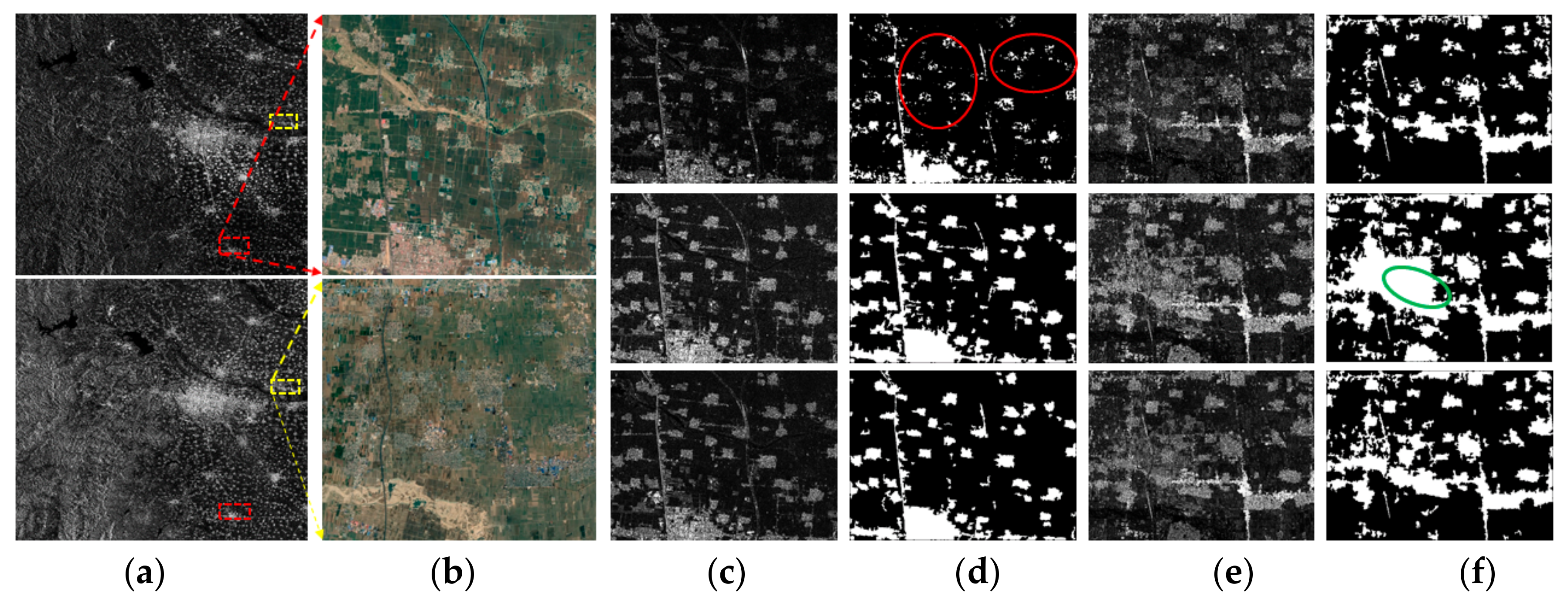
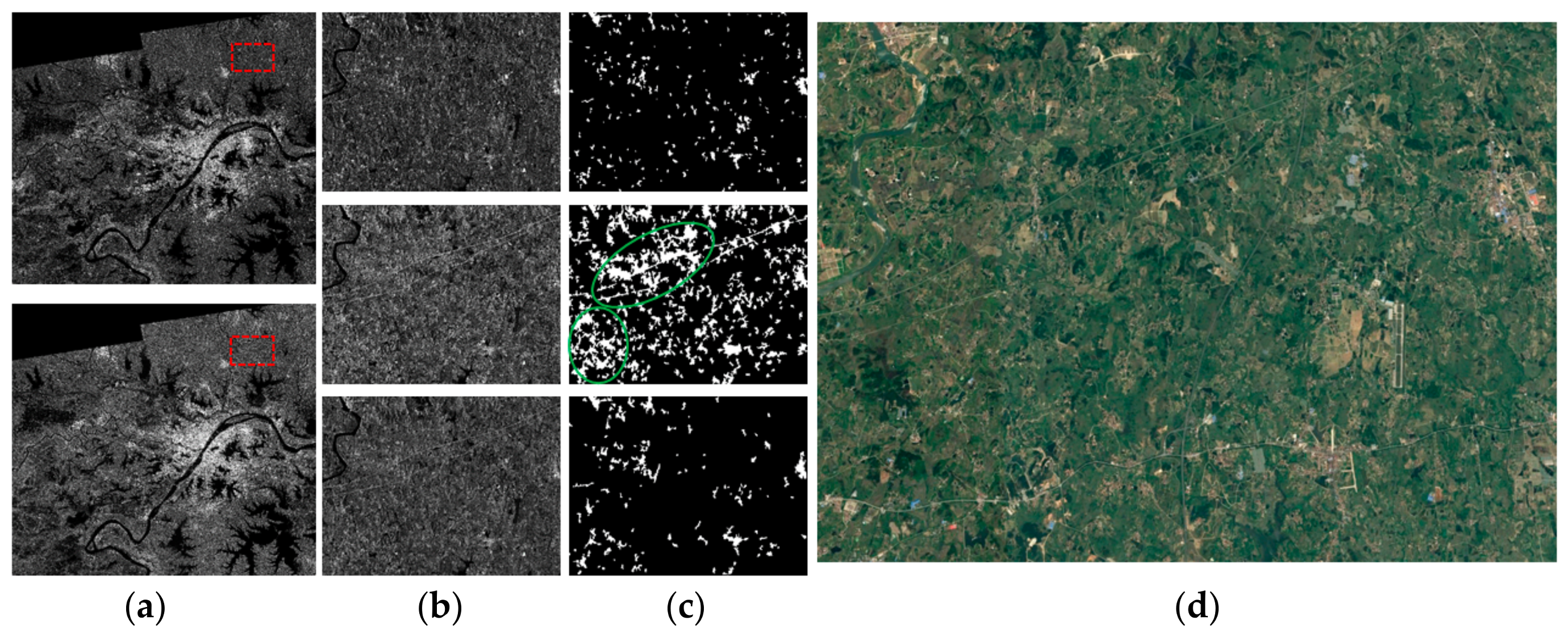
The BAs extraction approach is based on the Seeds Selection and Region Growing (SSRG) procedure. The points in SAR images which show high backscattering patterns and obvious textural patterns are chosen as seeds, and also considered as candidate BAs. The characteristics of these seeds include three parts: image intensity, local spatial indicator, and texture feature, respectively, and the region growing step is implemented independently from the three parts. BAs extraction results are obtained by merging the results obtained from the three SSRG procedures.

(a) Seed extraction:

The pixels with very high backscattering in SAR have a high probability of belonging to BAs, which are selected as the first part of the seeds. A threshold, namely $T_{s1}$, is applied to the whole image to obtain these seeds. $T_{s1}$ is a value set in the [0, 1] range which specifies a cutoff point of the maximum intensity (i.e., 255) for the seeds.

The second set of seeds is obtained from the local Getis-Ord $G_i$ index. $G_i$ is useful for determining clusters of similar values, where concentrations of high values result in a high value and concentrations of low values result in a low value [22]. The local Getis-Ord $G_i$ index is defined as

$$G_i=\frac{{\sum }_j{w}_{ij}{x}_j}{{\sum }_j{x}_j}, j\ne i.$$

(1)

where $x_j$ is the intensity value of pixel $j$. As shown in Equation (1), the calculation of the local $G_i$ index requires the spatial weight matrix $W$. Each weight element $w_{ij}$ in $W$ corresponds to a pair of observations at locations $i$ and $j$. $w_{ij}$ is set to 1 if the two locations show spatial interaction, and set to zero if the two locations indicate a lack thereof. There are three main forms of weight matrix, including Rook’s, Queen’s, and Bishop’s. In Rook’s matrix, $w_{ij}$ is set to 1 if the pixel $j$ shares a common edge with $i$; otherwise, it is set to 0. $w_{ij}$ is set to 1 if the pair shares a common vertex, or set to 0 otherwise in Bishop’s case. In Queen’s weight, $w_{ij}$ is set to 1 if the pair shares either a common edge or a vertex; otherwise, it is set to 0 [35]. In our work, the Queen’s case (i.e., the eight neighborhoods of the pivotal position $i$ are considered) is used to obtain more compact building area. The denominator $\sum _j{x}_j$ is the same for every pixel $i$ in the target image and can be neglected, so the $G_i$ index are actually the function of the eight neighborhoods of position $i$. In this case, the central pixel $i$ can be detected as long as it is surrounded by pixels with high intensities. As a result, the bright concentration and the “outliers”, i.e., pixels with low intensity surrounded by pixels with high values can all be detected by $G_i$. Thus, some areas with shadow effects or low levels of reflections can be identified using $G_i$ index, which is an alternative to using only image intensity. After computing the $G_i$ index, the $G_i$ map is stretched to a value range between 0 and 255. To obtain a second set of seeds, a threshold of $T_{s2}$ from [0, 1] is applied to the 8-bit gray-scale Getis-Ord $G_i$ map.

To get more precise BAs extraction mapping, texture features also need to be considered to extract BAs in areas with remarkable heterogeneity. For a single-polarized SAR image, integrating both texture measures and intensity has proven to be effective in classification [36,37]. The last set of seeds is obtained from variogram function-based texture feature. Compared with the traditional texture features derived from the gray level co-occurrence matrix (GLCM) and other classic texture-based methods, the variogram function-based textures provide greater efficiency and better results from SAR data [38]. The traditional semivariogram is defined as follows:

$$\mathsf{\gamma }\left(h\right)=\frac{1}{2N}\sum _{i=1}^N{\left(Z\left(x_i\right)-Z\left(x_i+h\right)\right)}^2$$

(2)

The variogram function-based feature used in this work is the simple deformation of (2), namely madogram, and defined as follows [39]:

$$\mathsf{\gamma }\left(h\right)=\frac{1}{2N}\sum _{i=1}^N\left|Z\left(x_i\right)-Z\left(x_i+h\right)\right|$$

(3)

where $Z\left(x_i\right)$ represents the image intensity at location $x_i$; $h$, called the lag distance, is a vector possessing both magnitude and direction, and $x_i+h$ represents the pixel located at distance $\left|h\right|$ to location $x_i$ in the vector direction. The madogram $\mathsf{\gamma }\left(h\right)$ is calculated in the neighborhood window of each pixel. $N$ is the number of pairs of pixels within $\left|h\right|$ distance apart in the vector direction within the window. Generally, the lag distance is defined as the value at which the $\mathsf{\gamma }\left(h\right)$ are no longer correlated when the semivariogram reaches a sill [40], which also applies to the madogram. This latter, taking the absolute values instead of measuring squares of all difference by the semivariogram, can also relate the variance of pixels to their spatial location and, characterize the spatial variability in a neighborhood, thus providing the same performance as that obtained from the semivariogram but with a much more level of lower computational complexity [41]. The optimal window size and lag distance were set to 9 × 9 and 3, based on trials seeking a tradeoff between accuracy and false alarms. Too large a window size will cause boundary effects, while too small a window size will fail to capture the texture structures. The $\mathsf{\gamma }\left(h\right)$ is calculated by averaging four directions set as 0°, 45°, 90° and 135°.

After computing the madogram, the associated map is also stretched to a value range between 0 and 255. To obtain the last set of seeds, a threshold of $T_{s3}$ set at [0, 1] is applied to the 8-bit gray-scale madogram map.

(b) Region growing:

The second step is region growing from the three parts of seeds extracted in step (a), respectively. For the seeds of intensity, the pixels in a window around the seeds that have a backscattering larger than a second intensity threshold, labelled $T_{u1}$, are included in the BAs map. Then, the newly added pixels are included in the intensity seeds, and the region growing step is iteratively implemented until no additional pixel can be added to the BAs map. The same region growing process separately applies to the $G_i$ seeds and madogram seeds using a second $G_i$ threshold and a second madogram threshold, namely $T_{u2}$ and $T_{u3}$. The window size is set at 3 × 3, since the possible size values between 3 and 7 make no difference to the result [33].

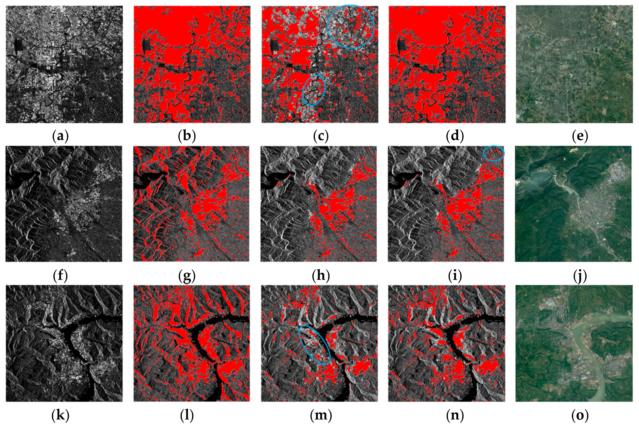
Three BAs extraction maps can be obtained through the three independent SSRG processes, and the result BAs map is obtained by merging the three maps using a logical operator OR. For the Sentinel-1 SAR data with a resolution approximately 5 × 20 m², the texture features are not obvious in dense urban areas, and image intensity can be used to extract most BAs. The Getis-Ord $G_i$ and madogram features are supplements to yield more precise BAs extraction results in areas with apparent textures (e.g., industrial zones with large, flat roofs). A more detailed analysis is provided in Section 4.1 for the determination of parameters $T_{si}$ and $T_{ui} ,i=1,2,3$.

3.3. Post-Processing

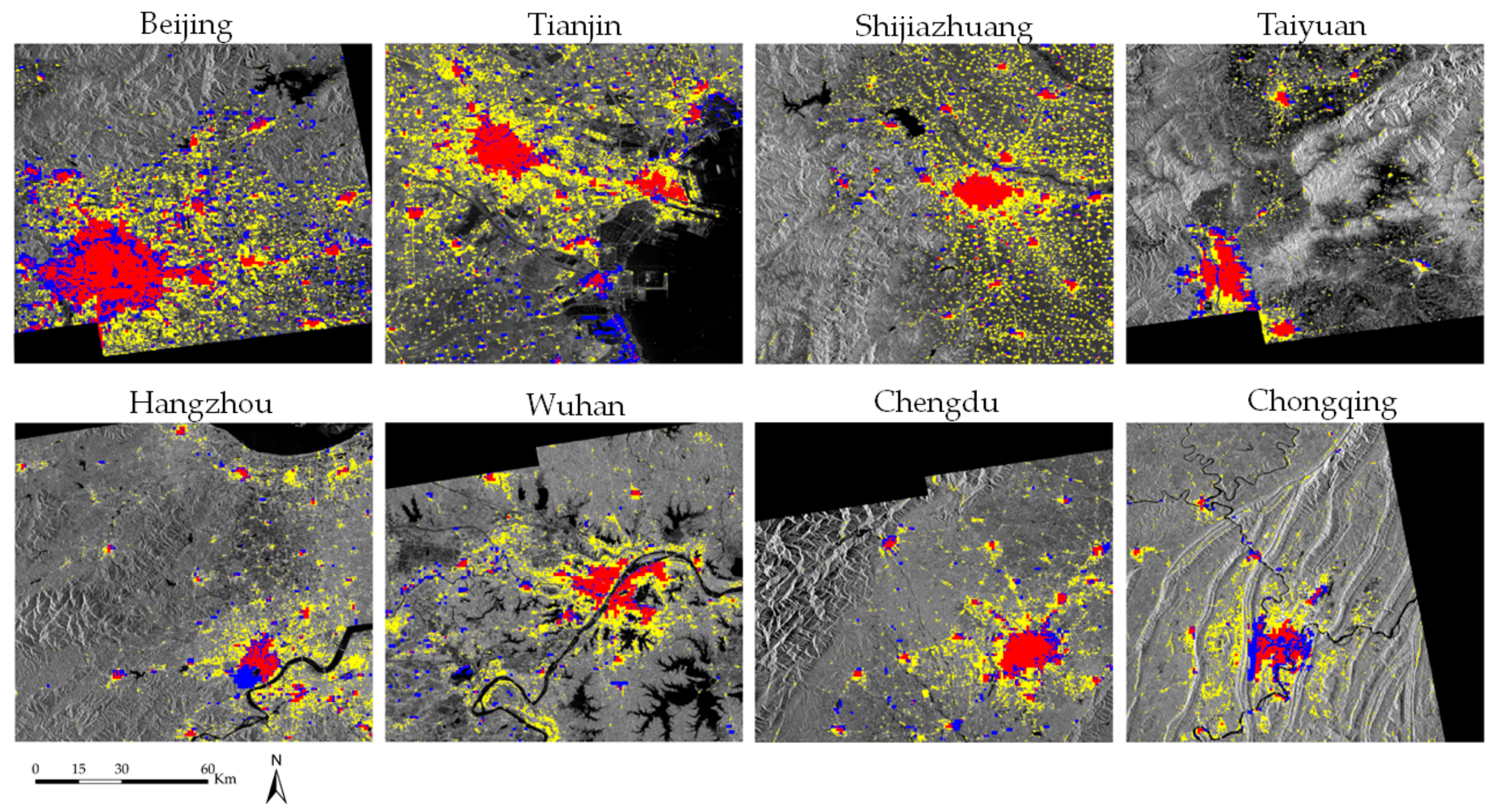
The last part of the framework (Figure 1) aims to remove false positives caused by mountains. The strong reflection due to foreshortening or layover effects in mountainous areas are highly likely to be misclassified as buildings, which significantly reduces the extraction accuracy. The most direct way to address this problem is to use digital elevation model (DEM) data to mask the mountain areas. Since buildings may also exist on high plateaus, we cannot use a unified threshold of DEM value to automatically mask the layover areas for all regions. Therefore, the slope factor needs to be considered. In a previous work [33], an empirically determined slope value (30°) was used to discard mountainous areas. This was based on the assumption that it is highly likely that high backscattering regions are due to hills and not to buildings, when the slope value is too large. Since this assumption is reasonable, our work is also based on this point.

In this step, a bilinear interpolation algorithm is first used to obtain a DEM map with the same space posting as that of Sentinel-1 data. Then, the slope is calculated inside a 5 × 5 pixel kernel. The slope map derived from DEM may be not accurate in each pixel of the SAR image for many reasons, such as inaccuracy of DEM data, or the resolution of the DEM. Thus, some pixels belonging to building areas may have a high slope, which would be filtered out by the slope map. To avoid this problem, the average slope value is computed in a 21 × 21 window around the pixel being tested [33], which is also the optimal window size for Sentienl-1 SAR data obtained through trials. Obviously, this step can be done independently before or after the BAs extraction process, and the slope threshold is different in areas with different terrains, i.e., 10° in plains or 15° in mountainous cities, based on a tradeoff between BAs commission error and omission error determined through multiple experiments in plains and mountainous areas.

Specifically, the Advanced Spaceborne Thermal Emission Reflectometer DEM (ASTER GDEM2) and the DEM based on the Shuttle Radar Topography Mission, as released by the Consortium for Spatial Information (SRTM CGIAR-CSI version 4.1), as two freely available global DEMs, are introduced for mountain masking. The possible errors due to these two DEMs are analyzed, as further detailed in Section 4.4.

After all of the above steps, a morphological operator with 3 × 3 pixel-size kernels is applied to the result to smooth the BAs borders of BAs.

4. Experiment Results

4.1. Derivation of Parameters

To identify the stable parameters presented in the previous section, various environments, such as high density residential areas, agricultural fields, and rural settlement areas in northern and southern cities were selected.

Figure 2(a1)–(d1) show the VV images and (a3)–(d3) show the VH images. The dependence of the overall user, and producer accuracy values for BAs obtained from parameters $T_{s1}$ and $T_{u1}$ using Figure 2(a3), are depicted in

Table 2. Overall accuracy (%)/user’s accuracy (%)/producer’s accuracy (%) as a function of $T_{s1}$ and $T_{u1}$.

	$T_{u1}$	0.1	0.2	0.3	0.4	0.5
$T_{s1}$
0.3		69.9/66.2/98.4	79.1/75.9/93.9	82.3/83.4/86.8
0.4		70.0/66.3/98.4	80.1/77.1/93.5	82.7/85.2/84.9	81.1/88.8/77.1
0.5		70.0/66.3/98.3	81.0/78.2/93.1	82.8/86.3/83.7	80.5/89.9/74.8	77.1/92.2/66.2
0.6		70.2/66.5/98.3	81.6/79.0/92.9	83.0/87.3/82.8	80.0/90.4/73.3	75.9/92.5/63.7
0.7		70.2/66.5/98.3	81.6/79.1/92.8	83.1/88.1/82.0	79.6/91.0/72.0	75.2/92.9/62.0
0.8		70.2/66.5/98.3	81.9/79.5/92.8	83.1/88.7/81.4	79.3/91.5/71.0	74.4/93.2/60.4
0.9		70.5/66.7/98.3	82.1/79.7/92.8	83.3/89.0/81.2	79.1/91.7/70.3	74.2/93.2/59.9
1		70.5/66.7/98.3	82.1/79.7/92.7	83.4/89.5/81.0	78.9/91.9/69.7	73.8/93.4/59.1

. We can see that selecting the proper $T_{u1}$ is key for obtaining a better results. The overall accuracy, and the user’s and producer’s accuracy all reached at least 80% when $T_{u1}$ was 0.3 (see Table 2). We aimed to select the parameters by seeking a tradeoff among the three accuracy values, so $T_{u1}$ was set as 0.3. When considering all three accuracies, we focused more on user’s accuracy (i.e., we hoped to obtain the BAs extraction result with as few false alarms as possible). The selection of $T_{s1}$, with a range of value from 0.3 to 1, had little effect on overall accuracy, but made a difference in the user’s and producer’s accuracies. The user’s accuracy increased and the producer’s accuracy decreased, as $T_{s1}$ increased from 0.3 to 1. We set the $T_{s1}$ as 0.8, as the variation of $T_{s1}$ from 0.8 to 1 made little difference in the user’s accuracy. By test comparison, the selection of $T_{s1}$ and $T_{u1}$ was not critically fixed to 0.8 and 0.3, and did not really affect the final result when the parameters were allowed to fluctuate by plus or minus 0.02. For Sentinel-1 data with an approximately 20 m resolution, the procedure based on image intensity could detect most of the BAs.

The threshold parameters of the Getis-Ord $G_i$ and madogram were also obtained from experiments using only $G_i$, and only the madogram with results shown in

Table 3. Overall accuracy (%)/user’s accuracy (%)/producer’s accuracy (%) as a function of $T_{s2}$ and $T_{u2}$.

	$T_{u2}$	0.1	0.2	0.3	0.4	0.5
$T_{s2}$
0.3		68.7/65.9/95.8	80.4/78.3/91.5	83.1/87.9/82.1
0.4		68.8/65.9/95.8	81.2/79.3/91.4	83.1/88.3/81.6	78.0/92.4/67.7
0.5		68.8/65.9/95.8	81.4/79.6/91.4	83.1/88.9/81.0	77.7/92.7/66.9	69.1/94.7/49.6
0.6		68.8/65.9/95.8	82.0/80.3/91.4	83.7/89.9/80.9	77.6/93.1/66.4	68.6/94.8/48.5
0.7		68.8/65.9/95.8	82.1/80.6/91.2	84.0/90.8/80.6	77.4/93.6/65.6	67.8/94.8/47.2
0.8		68.8/65.9/95.8	82.1/80.6/91.2	83.8/91.3/79.7	76.7/93.8/64.0	66.9/94.8/45.6
0.9		68.8/65.9/95.8	82.1/80.6/91.2	83.4/91.8/78.5	76.6/94.2/63.6	66.0/95.0/43.7
1		68.8/65.9/95.8	81.3/81.5/87.8	82.1/92.4/75.4	73.4/94.3/57.7	59.5/94.3/32.2

and

Table 4. Overall accuracy (%)/user’s accuracy (%)/producer’s accuracy (%) as a function of $T_{s3}$ and $T_{u3}$.

	$T_{u3}$	0.1	0.2	0.3	0.4	0.5
$T_{s3}$
0.3		60.9/61.0/90.9	71.4/69.4/90.8	80.7/80.6/87.9
0.4		60.9/61.0/90.9	71.4/69.4/90.8	81.0/81.0/87.8	81.6/89.2/77.7
0.5		60.9/61.0/90.9	72.0/70.0/90.8	81.4/81.5/87.8	81.5/89.4/77.3	70.0/94.3/51.4
0.6		60.9/61.0/90.9	72.0/70.0/90.8	81.4/82.8/85.8	81.1/89.8/76.1	69.2/94.2/50.0
0.7		60.9/61.0/90.9	71.6/70.2/88.8	81.1/84.8/82.3	80.2/91.2/73.0	68.0/95.3/47.1
0.8		60.9/61.0/90.9	71.6/70.2/88.8	81.1/84.8/82.3	72.9/92.7/58.0	46.8/89.8/9.6
0.9		60.9/61.0/90.9	71.6/70.2/88.8	81.1/84.8/82.3	72.9/92.7/58.0	46.8/89.8/9.6
1		60.9/61.0/90.9	71.6/70.2/88.8	81.1/84.8/82.3	72.9/92.7/58.0	46.8/89.8/9.6

. Being different from the selection of $T_{s1}$ and $T_{u1}$, we selected $T_{s2}$, $T_{u2}$, $T_{s3}$ and $T_{u3}$ by first considering the user’s accuracy, since the image intensity detected most of the BAs, and the other two features were only supplements in areas with obvious textures. We hoped to minimize the commission error and boundary effect caused by these two features. According to Table 3, we set $T_{u2}$ as 0.5 when the user’s accuracy reached more than 94.5%. It made little difference when $T_{s2}$ was varied from 0.6 to 0.9, so we set $T_{s2}$ as 0.6 to maximize the overall and producer’s accuracies. Based on same rule, $T_{s3}$ and $T_{u3}$ were set as 0.7 and 0.5, according to Table 4.

The optimal parameters trend obtained using Figure 2(a3) as a test case was similar to that found using Figure 2(b3),(d3) and VV polarization images (a1)–(d1). For strongly vegetated growing areas, larger $T_{u1}$ and $T_{u2}$ values, such as 0.35 and 0.55, could be selected. The parameters for the madogram were fixed, since they only characterize the spatial variability.

4.2. The Influence of Polarization Information in BAs Extraction

The building structures are different over China, e.g., rural settlements are bungalows and are intensively distributed in north, while those are small buildings and scattered in south. To study the effects of different polarizations on the BAs extraction results in various environments, the proposed method is applied to the VV and VH images in the four test sites. VV and VH polarized images are known to emphasize the double-bounce effect and volume scattering, respectively. In the work of [31], urban extraction could be further improved when the results from C-HH and C-VV were combined with the OR operator, while a combination of C-HH and C-HV reduced the accuracy [42]. In [42], the accuracy obtained from HH image was higher than the combination of C-HH and C-HV results, which indicates that the single cross-polarized channel is not suitable for BAs extraction, and that the operator OR will accumulate commission errors. Based on these previous studies, instead of fusing the results of the two channels, we tried to use an averaged image of VV and VH images to extract BAs, because the averaging of VV and VH can compensate for the different scattering geometry of buildings, since different orientations of the buildings lead to diverse backscattering in VV and VH. The images of VV, VH and the averages of the two channels are shown in Figure 2(a1)–(d1),(a3)–(d3),(a5)–(d5), respectively. The overlay results of VV, VH, and averaged images are shown in Figure 2(a2)–(d2),(a4)–(d4),(a6)–(d6), respectively. Optical images of the four test sites from a Google Earth map are illustrated in (a7)–(d7), and (a8)–(d8) show the reference ground truth built-up area maps obtained by a visual interpretation of a high-resolution Google Earth map. Quantitative results from the test sites are reported in

Table 5. Accuracy of four test sites using the proposed method.

	Test Site 1			Test Site 2			Test Site 3			Test Site 4
	VV	VH	Ave.	VV	VH	Ave.	VV	VH	Ave.	VV	VH	Ave.
Kappa	0.62	0.68	0.70	0.43	0.35	0.56	0.57	0.74	0.76	0.47	0.25	0.39
OA %	81.2	84.2	85.3	89.2	82.2	91.9	88.9	91.5	92.6	93.0	82.6	88.7
UA %	89.5	89.0	90.1	36.3	27.0	45.8	88.1	74.1	82.9	45.	21.5	32.1
PA %	76.7	82.9	84.1	71.9	91.0	86.8	49.2	85.5	77.8	57.1	66.7	71.5

Ave. refers to the averaged image from VV and VH images.

.

For the high-density housing area shown in Figure 2(a1),(a3), both VV and VH image are classified as good results, with a kappa coefficient at 0.62 and 0.68. Usually, a kappa value greater than 0.6 indicates a good classification quality. The VH channel showed slightly better performance than the VV channel. The strong response in the VH channel indicated that the buildings were oriented at 45 degree with respect to the satellite flight path. The result from the averaged image improved the results slightly more than the VH channel, due to some areas with high VV values and low VH values. The different orientations of the buildings led to diverse backscattering in VV and VH. In this case, a slightly better result was obtained using VH; it is possible that an opposite result would be obtained in areas in which most buildings are parallel with satellite flight path.

Subset tests 2 and 3 are rural areas selected from Tianjin city in northern China. Subset 2 is an agricultural field, and a few rural buildings are scattered, as seen in Figure 2(b7), while subset 3 is a rural residential area. The vegetated regions in the VH image showed higher backscattering than in the VV image, which result in more false alarms (see Figure 2(b4). The rural buildings in VV showed low backscattering, and producer’s accuracy (71.9%) using VV data was not better than that obtained using VH data (91.0%). A more obvious comparison of VV and VH images in rural settlements is illustrated in Figure 2(c1),(c3). The averaging of strong VH backscatter from vegetation fields and the weak VV backscatter from rural houses improved the result, with a 0.13–0.21 improvement in kappa, as shown in Figure 2(b6). The result from averaged image of two channels greatly increased the overall and user’s accuracy over that of VV or VH, although it yielded a slightly decrease in producer’s accuracy. Subset 3 also indicated the low backscattering of rural houses in the VV image, and the averaged image can greatly improve the result. To provide more validation, a visual comparison of Shijiazhuang city is shown in Figure 3. The results from two ROIs (the red and yellow rectangles shown in Figure 3a) yielded the same issue: the VV image resulted in some omission errors (shown in red circle in Figure 3d) in rural areas, and the VH image resulted in some commission errors (shown in green circle in Figure 3f) in vegetation areas. It needs to be stressed that the images were all selected in the early vegetation season, and that only small areas showed high backscattering in VH. For strong vegetation fields in the late stage of the vegetation season, both VV and VH may show very high backscattering in different vegetation fields.

The fourth subset is the rural area of Hangzhou city with many dispersedly distributed houses. For this situation, the most precise BAs extraction map was obtained from the VV channel. The result from VH showed a high commission error with user’s accuracies as low as 21.5%, and the averaged image still resulted in a low user’s accuracy. The visual comparison of Wuhan city is illustrated in Figure 4. The ROI region also validates the advantage of the VV image in BAs extraction. Some commission errors occurred in the green circle in the VH image, and omission errors occurred when the averaged image was used. These results indicate that in southern China, the VV image is more suitable for BAs extraction with higher accuracy.

4.3. Comparison with Other Methods in BAs Extraction

In the work presented by [33], the building area was successfully extracted based on image intensity using 75 m-resolution ASAR Wide swath data, but for 20 m-resolution Sentinel-1 SAR data, some areas, e.g., industrial areas with wide flat roofs, could not be completely detected.

To study the effect of adding the other two features (Getis-Ord and madogram), a subset VV polarization image with 600 × 600 pixels in the industrial region of Chengdu city was selected for testing. We also compared the results with those of the BAs extraction map obtained by direct thresholding, i.e., using a logical OR operator on three threshold maps based on $T_{ui},i=1,2,3$. Validation points of true BAs and non-BAs were randomly selected throughout the image based on high resolution Google Earth images. The validation data contained 1000 pixels of BAs and non-residential areas respectively.

Table 6. Accuracy comparison of results of the proposed method, region growing using only intensity, and thresholding method.

Method	Kappa	Overall Accuracy (%)	BAs Commission Error (%)	BAs Omission Error (%)	Exec. Time (s)
Intensity-based SSRG	0.82	91.2	0	17.6	1.6
Proposed method	0.97	98.6	0	2.9	3.5
Thresholding	0.95	97.6	3.4	1.4	3.0

displays the comparison results including the accuracies and execution time of the three methods.

The texture feature was obvious in the industrial area, since low backscattering occurred due to specular reflection of roofs, as shown in Figure 5a. In this case, some flat roofs could not be detected by using only intensity in the region growing procedure, and high numbers of omission errors (17.6%) were obtained, as shown in Figure 5b, although this shows the best execution time performance (1.6 s). By adding the other two features, most of the BAs that were not detected by intensity alone could be identified as the yellow areas shown in Figure 5c, and a higher kappa coefficient (0.97) was achieved. The thresholding map based on $T_{ui},i=1,2,3$ showed a higher commission error (3.4%) due to some vegetation and bail soil, as a number of red speckles in Figure 5d show, and a lower kappa (0.95) than that of our result. However, no commission error occurred based on the proposed method.

4.4. Mountain Masking Test Using Different DEM Data

A detailed comparison of the effect of two commonly used DEMs (ASTER GDEM2 and SRTM DEM) in mountain masking is presented in this section. The SRTM DEM data cover the earth between latitudes 60°N to 57°S, with an approximately 90 m resolution. The global ASTER GDEM2 data cover the land surface between 83°N and 83°S, with approximately 30 m grid cell size. We aim to use the DEM data to mask the whole image automatically, so we chose areas with different terrains, such the flat urban areas, a plain area surrounded by mountains, and a mountainous area, to evaluate the possible errors using two DEMs.

Figure 6a shows the urban center in Chengdu City located in the Sichuan basin. Since no mountains exist in this region, the BAs extraction map without masking is displayed in Figure 6b, with no false alarms due to mountains. For this flat terrain, an empirically determined value (10°) is used for two DEMs. Figure 6d shows a similar result to that in Figure 6b, which indicates that masking using SRTM DEM does not reduce the effectiveness of the result. The mask result using ASTER GDEM2 masks the building areas on the right, which greatly reduces the accuracy, as shown in Figure 6c. This indicates that SRTM DEM produces accuracy superior to that of ASTER GDEM2, which has also been noted previously [43,44]. One study [43] implied that SRTM has a higher vertical accuracy than that of ASTER-GDEM2, and that the underestimation of ASTER-GDEM2 is more pronounced on flat and less complex terrains. Thus, the slope map derived from SRTM also has a higher accuracy than that derived from ASTER GDEM2 through interpolation and slope calculation. Under the same slope threshold in the flat urban area, the results reveal that the mask result using SRTM could retain the built-up areas well, but that the ASTER GDEM2 may mask off the BAs.

The second test area is Dujiangyan city as shown in Figure 6f. It consists of a plains area surrounded by mountains. Figure 6g displays the BAs extraction map without the mask. Unsurprisingly, most of the mountain areas are misclassified as BAs, which significantly reduces the extraction accuracy. For this case, with buildings located in the plains region, the slope threshold is also set to 10 degrees for the two DEMs to evaluate the results. A visual comparison based on the two DEMs is offered in Figure 6h,i, which indicates approximately the same result. The top right part of Figure 6i shows that the results using SRTM have a few more false alarms than the results based on ASTER GDEM2, as shown in Figure 6h.

The last sub-area example is a mountain region in Chongqing city, shown in Figure 6k. The buildings of this area are built on mountains with complex terrains and a large slopes. The results shown in Figure 6l also display poor results without mountain masking. Since the area has a high level of topographic relief, 15° is set as the slope threshold. The masking result using ASTER GDEM2 shown in Figure 6m shows fewer false alarms, but still causes more omissions than the result using SRTM DEM, shown in Figure 6n, which can be seen in the cyan circle on Figure 6m. Mountain masking based on SRTM DEM can provide a more precise BAs map than that using ASTER GDEM2.

4.5. Comparison of BAs Extraction by the Proposed Method and Optical Data

The BAs extraction overlay results of the eight cities using the proposed method are shown in Figure 7, with red indicating residential areas. Among the results, the averaged images of two polarizations are used for northern cities in Figure 7a–d, and the VV images are used for southern cities in Figure 7e–h, based on the analysis in Section 4.2. SRTM DEM data are used for the mountain masking step according to the conclusion of the above section. The slope threshold is set to the experience value of 15° for the mountainous city (Chongqing), and 10° for other cities. The images sizes are all approximately 7000 × 6000, and the execution time of each image is approximately five minutes in C++ for the whole procedure, including BAs extraction and post-processing (interpolation of DEM data, computation of slope, mountain masking, and morphological operation).

4.5.1. Comparison with GlobCover

To give a quantitative assessment, the results are compared with the GlobCover urban product, which has a spatial posting at approximately 300 m. The resulting maps obtained by the proposed method are downsampled to maps, with the same spatial posting as GlobCover using a previous described method in [33], i.e., a spatial majority voting method is performed. Validation data points of true BAs and non-BAs are randomly selected throughout the image based on optical Google Earth images acquired in 2010 through visual interpretation. This comparison is based on the assumption that the building areas did not disappear in the 7-year interval. The validation data of every city contain 1000 pixels for BAs and non-BAs. Among them, the built-up samples contain the city center points, rural houses, buildings in bail soil, and the buildings in the mountains, especially for Chongqing city. The non-residential validation data contain water areas, bail soil, vegetation fields, forests, high mountains, and low hills.

Table 7. Accuracy comparison of results based on proposed method and GlobCover urban map.

Cities	BAs Extraction	Kappa	Overall Accuracy (%)	BAs Commission Error (%)	BAs Omission Error (%)
Beijing	Proposed	0.98	99.3	0.5	1.0
	GlobCover	0.35	67.4	24.3	49.5
Tianjin	Proposed	0.96	98.2	0.6	3.0
	GlobCover	0.46	73.0	1.3	53.4
Shijiazhuang	Proposed	0.98	99.5	0	1.1
	GlobCover	0.56	77.9	0.5	44.0
Taiyuan	Proposed	0.86	93.5	0	13.1
	GlobCover	0.36	67.8	6.4	61.9
Hangzhou	Proposed	0.95	97.7	0.1	4.6
	GlobCover	0.38	69.0	9.4	57.6
Wuhan	Proposed	0.88	94.3	8.7	2.2
	GlobCover	0.45	72.6	1.3	54.3
Chengdu	Proposed	0.95	97.6	0.1	4.8
	GlobCover	0.34	67.0	4.6	64.4
Chongqing	Proposed	0.84	92.2	3.2	12.9
	GlobCover	0.43	71.8	13.9	48.4
Average	Proposed	0.92	96.5	1.65	5.34
	GlobCover	0.42	70.8	7.71	54.2

illustrates the results of a comparison to the GlobCover urban product.

From Table 7, we can see that the proposed method produces better results in all cities than GlobCover, with a kappa coefficient ranging from 0.84 to 0.98, and an averaged kappa of 0.92, while the results of GlobCover obtain poor BAs detection, with a kappa lower than 0.6 and averaged omission error amounting to 54.2%. To show a more direct comparison with GlobCover urban product, the downsampled results of the proposed method are overlaid on GlobCover urban area maps in Figure 8. The yellow parts denote the BAs detected by the proposed method and missed by GlobCover, with large areas shown in Figure 8. It needs to be stressed that these yellow areas comprise two parts: one is the BAs due to the urban expansion during the 7-year interval, while the other is due to the undetected BAs of GlobCover which were actually present on the ground in 2009. According to the latest World Urbanization Prospects [45], in many parts of the world, the growth rate in urban built-up areas is faster than its rural counterpart. Thus, in peri-urban areas, most yellow areas may be due to urbanization which occurred from 2009 to 2017, i.e., these BAs detected by SAR were not present on the ground in 2009, with high probability. Most yellow parts in rural regions were already present on the ground in 2009, with high probability, but could not be detected by GlobCover. Since the validation samples we selected were all from the 2009 true map, the quantitative evaluation was objectively true.

For Beijing, GlobCover misclassifies most urban parks as BAs, and yields the highest commission error (24.3%). However, our results do not contain these areas, as shown in the blue region of the urban area of Beijing in Figure 8. The GlobCover map misses most of the suburban residential areas in Beijing, and the same occurs in Tianjin city, as shown in Figure 8b, while our results also miss some small towns. The result obtained in Shijiazhuang in Figure 8 show that most rural residential blocks cannot be detected in GlobCover, with an omission error of 44%, while the proposed method using the averaged image of VV and VH channels shows good detection results in rural areas, and no commission errors in the 1000 test points. It is worth noting that small buildings are undetected due to the resolution of 300 m. For Hangzhou city, GlobCover shows an obvious commission error in the hilly land close to the West Lake, with the commission error amounting to 9.4%, as the large blue patch in Hangzhou result map in Figure 8 illustrates. The result of Wuhan city by the proposed method shows some commission errors in the agricultural area on the beach of Yangtze River, located to the south of the urban center, with the largest commission error reaching 8.7%, and misses some small towns in rural places due to the occasional weak double-bounce backscattering of rural houses. GlobCover shows some omission errors in the Wuhan urban area, and commission errors due to water bodies and vegetation areas, while our result shows good performance in urban areas. The same occurs in Chengdu city, where the vegetation areas in the northeast of the urban center are detected as BAs in GlobCover. The worst results of the proposed method are from Taiyuan and Chongqing, with the highest omission errors (13.1% and 12.9%, respectively). The omission errors in these two cities are mainly caused by the mountain masking step, wherein a small portion of BAs built on complex terrain with slope values larger than the slope threshold are masked. A higher slope threshold may cause fewer omission errors, but this can increase commission errors in mountainous areas. The commission areas of Chongqing city are due to the presence of mountainous areas. The GlobCover results also miss some suburban BAs, and commission errors occur in some bail soil fields located on hills.

4.5.2. Comparison with Landsat-8 OLI/TIRS Data-Based BAs Extraction

One northern city (Beijing) and one southern city (Wuhan) are chosen as the test sites for comparison with Landsat-8 data-based BAs extraction. The Landsat-8 OLI/TIRS images (Beijing: 28 September 2017; Wuhan: 26 July 2017), having a spatial resolution of 30 m, were carefully selected (i.e., less cloud coverage during the growing season) from U.S. Geological Survey: http://earthexplorer.usgs.gov/. The radiometric calibration and atmospheric correction are conducted for Landsat-8 images in the Environment software. The BAs extraction results from Landsat-8 images are obtained by the method developed in [46]. Figure 9a and c display the Landsat composites with BAs extraction results overlaying on them. The BAs results of our work were also resampled to align with Landsat data of 30 m resolution by spatial majority, and the two results overlaid on resampled SAR images are available in Figure 9b,d. Ten thousand validation samples of true BAs and non-BAs are randomly selected based on optical Google Earth images acquired in 2017 through visual interpretation, and their quantitative evaluation is displayed in

Table 8. Accuracy comparison of SAR-based and Landsat-based BAs extraction.

City	BAs Extraction	Kappa	Overall Accuracy (%)	BAs Commission Error (%)	BAs Omission Error (%)
Beijing	Proposed	0.82	91.4	3.64	13.9
	Landsat-8	0.86	93.2	10.6	1.79
Wuhan	Proposed	0.78	88.94	9.7	12.6
	Landsat-8	0.70	84.49	23.2	0.89

.

The overall accuracy in Beijing is 91.4%, to be compared with a slightly higher 93.2% for the Landsat-based result, which is the opposite in Wuhan (88.94% of SAR-based and 84.49% of Landsat-based), as shown in Table 8. Large portions of bare lands, and some areas with low vegetations (e.g., the uncultivated land on the beach of Yangtze River) are confused as BAs in Landsat images, increasing the commission error (10.6% in Beijing and 23.2% in Wuhan), while some buildings in strongly vegetated areas and areas covered by cloud are not detected (omission error is 1.79% in Beijing and 0.89 in Wuhan). The commission errors of our results occur in some vegetation area. Due to some building areas with low backscattering, higher rates of omission errors (13.9% in Beijing and 12.6% in Wuhan) are achieved than with Landsat-based results.

5. Discussion

As shown by the comparison results, the SSRG based on intensity, spatial association indicator, and texture feature can yield more precise BAs maps in large, flat-roof building areas compared with the SSRG method using only intensity. The proposed method can also largely avoid false alarms compared with the thresholding method based on the same three features, although it consumes slightly more time (3.5 s). This implies that the BAs map, obtained by region growing starting from selected buildings seeds with relative high feature thresholds ($T_{si},i=1,2,3$), can successfully avoid the isolated non-BAs with feature values between $T_{ui}$ and $T_{si}$($i=1,2,3$), which are falsely detected as BAs based on directly thresholding method using thresholds $T_{ui}$($i=1,2,3$). The main disadvantage of the proposed method is the essential need of strong backscattering in building areas. The buildings with high backscattering are crucial for selecting candidate BAs. If most buildings show similar radar signatures to their surroundings, a large area of omission will occur. Another disadvantage is the parameter optimization based only on 5 × 20 m² resolution Sentienl-1 data. Future work will be focused on the adaptive selection of thresholds based on data from different satellite SAR with different resolutions.

Compared with the GlobCover urban map with average accuracy 70.8% in validation points, the proposed method in Sentinel-1 5 × 20 m² resolution data achieves consistently better results (96.5%) in eight cities with different environments. The commission errors (7.71%) of GlobCover are mostly due to vegetation parks in urban areas, while our results successfully leave out these areas in most cities. Partly attributed to the 300 m resolution, the GlobCover urban maps miss out most rural BAs, yielding very high average omission error levels (54.2%), as opposed to 5.34% in our results. This indicates that the Sentinel-1 SAR data, with approximately 20 m resolution, has a distinct advantage on the extraction of rural BAs. The false alarms of our results are due to some agricultural fields, e.g., the crops on the banks of the Yangtze River. Although some detection errors occur by the proposed method, consistently accurate BAs map are achieved in both urban and rural regions on cities with different topographies in China. Compared with Landsat 8-based BAs extraction, the bare lands or lands with low vegetation coverage can be effectively distinguished from BAs in SAR by the proposed method, but are easily confused in Landsat images. For multi-cloud and rainy areas (e.g., southern China), Sentinel-1 SAR data are good options for BAs extraction on large spatial scales, due to the hard collection of optical images with low cloud coverage during the growing season. Although vegetation land is easily confused with BAs in SAR, these false alarms can be removed by coherence maps obtained by multi-temporal SAR images, because certain types of vegetated areas are not coherent in time. Since both SAR and optical data have their own merits and limitations, the fusion of SAR and optical data can overcome the deficiencies associated with a single sensor, and has been investigated in [47,48,49]. In the future, the fusion of SAR and optical data will also be considered in BAs extraction, in order to get more precise BAs map in large area, e.g., Sentinel-1 SAR based BAs extraction based on this work under a predefined mask of non-BAs areas, with the help of indexes (e.g., NDVI, NDWI, and so on) derived from Landsat scene or Sentinel-2A data.

Considering the influence of different polarizations in BAs extraction, the results show that the averaged image of two polarizations is more suited for BAs extraction in northern cities of China, and the VV image is suitable for BAs extraction in southern cities of China. In the selection of DEM for mountain masking, the results demonstrate that mountain masking using SRTM DEM leads to a more precise BAs map when Sentienl-1 SAR data with a resolution of 5 × 20 m² are used. Nevertheless, ASTER GDEM2 can be used as a fairly good data base over areas that are not covered by SRTM DEM (between 60°N and 83°N and between 57°S and 83°S).

6. Conclusions

In this paper, an operational and efficient built-up areas extraction framework for cities in China using Sentinel-1 SAR data has been introduced. Unlike traditional feature thresholding methods, or only intensity-based methods, spatial indicator and texture feature together with intensity are introduced in the seeds selection procedure for region growing, in order to obtain a BAs map. The proposed method shows higher accuracy (98.6%) in a subset industrial zone, compared with intensity-based SSRG method and thresholding methods. A quantitative evaluation in eight test sites suggests that the proposed approach shows strong ability in BAs extraction compared with GlobCover urban product in both urban and rural areas, and performs better in distinguishing BAs with bare lands and areas with low vegetation compared with Landsat 8 data-based results, which verifies the validity and robustness of the proposed framework.

Moreover, two polarizations and the averaged channel of Sentinel-1 data are employed to compare the results for different environment and building structures in China. The conclusion is that, for the southern cities with mainly small-scale and scattered settlements, the VV image is better suited for BAs extraction. The extraction based on the averaged image of VV and VH channels can improve the extraction accuracy in the northern China when the images are carefully selected at the beginning of the plant growing season. In addition, two global freely available DEMs are introduced to compare the effects of the mountain masking procedure. The results show that mountain masking based on SRTM DEM data yields more precise BAs maps than those produced using ASTER GDEM2.

These findings indicate that operational built-up areas mapping in China using Sentinel-1 SAR data is possible, which also lays the groundwork for successful global BAs mapping.