1. Introduction
Accurate localization in the underwater environment is crucial for a variety of applications such as monitoring of equipment deployed underwater (e.g., autonomous underwater vehicles—AUVs, towed devices) [
1], marine mammal behavioral studies [
2], security monitoring of divers, search and rescue operations (e.g., search for black boxes—voice and data recorders) following accidents at sea [
3], etc.
Sound, in contrast to light and electromagnetic waves in general, propagates efficiently in the ocean interior, because acoustic waves are subject to low absorption in water. Spatial variations of the sound speed in the water cause refraction (bending of acoustic rays) which in turn gives rise to shadow zones, caustics, and multipath [
4]. Multipath—multiple acoustic paths connecting a source and a distant receiver—may act as an information multiplier: the different arrivals at the receiver convey information from different water layers, whereas the reflected/refracted path geometries produce larger virtual apertures leading to resolution enhancement.
Existing underwater acoustic systems for pulsed source localization rely on hydrophone arrays which are either towed or independently deployed. The simplest towed array configuration involves two hydrophones which can provide source bearing estimates by measuring the time difference of arrival (TDOA) between the direct arrivals at the two hydrophones [
5,
6]. By combining bearing estimates from multiple hydrophone pairs located in a three-dimensional (3D) space, range and depth estimates can be obtained [
7]. Multi-element arrays [
8,
9] have the advantage of SNR improvement through beamforming and also allow for localization, e.g., by combining bearing measurements from spatially separated apertures [
9], by using backpropagation techniques [
10], or by applying methods based on the waveguide invariant [
11,
12] and the array invariant [
13,
14].
By exploiting TDOAs between direct and surface-reflected arrivals at a pair of hydrophones of known depths, 3D localization of pulsed sources can be achieved, subject to left–right ambiguity with respect to the vertical plane through the hydrophones. Under the assumption of negligible refraction effects (straight line propagation) the localization problem can be solved analytically [
15,
16]. Refraction effects become significant for localization at long ranges, typically longer than 1 km depending on sound speed characteristics and source/receiver positions. A number of ray-theoretic methods for two-hydrophone localization have been introduced [
17,
18,
19,
20] accounting for refraction effects on ray geometry and travel times.
In the framework of a recent study [
20], a Bayesian formulation has been introduced accounting for uncertainties of the arrival times and hydrophone locations, as well as for depth-dependent uncertainties in the sound speed profile, and using these to provide estimates for localization uncertainty. In this approach, which is based on ray theory, the depth and range (horizontal distance) estimation problem is decoupled from the bearing (azimuth) estimation problem, and the localization is carried out in two steps. In the first step, the depth and range of the source from each hydrophone is estimated by applying an iterative linearized Gauss–Markov inversion scheme. In the second step, the estimated ranges are combined with the hydrophone locations in the horizontal, if these are known, for the estimation of the source bearing. The advantage of this two-step approach is that the estimation of source ranges and depth relies on the knowledge of the hydrophone depths but not of their position in the horizontal, so the first step can be applied even if the horizontal locations of the hydrophones are not known.
To assess the performance of the Bayesian localization scheme, two experiments were conducted in December 2014 and June 2015 in the Eastern Mediterranean Sea off the north and south coast of Crete, in shallow and deep water, respectively. In the first experiment the focus was on localizing a controlled source (pinger), whereas the second experiment involved both pinger and sperm whale localization. This work reports on the results from the two localization experiments and is organized as follows:
Section 2 gives a summary of the Bayesian localization framework introduced in [
20]. The setup of the localization experiments is described in
Section 3.
Section 4 presents measured data and localization results. Finally,
Section 5 contains a discussion and conclusions from this work.
2. Bayesian Localization
Direct and surface-reflected acoustic arrivals from a pulsed source of unknown location and depth are picked up by two hydrophones H1 and H2 in a refractive environment characterized by a depth-dependent sound speed profile but assuming range independence. If the hydrophone depths and the sound speed profile are known, from independent measurements, the range and depth of the source can be estimated from the three TDOAs, between direct and surface-reflected arrivals at each hydrophone and between direct arrivals at the two hydrophones [
20]. This approach is based on ray theory and makes no assumption concerning the distance of the source from the hydrophones, i.e., the method is applicable even in cases where the source is in the vicinity of the two hydrophones. In the following, a brief presentation of the localization method is given.
The hydrophone depths are assumed known, from measurements, within some uncertainties. To account for these uncertainties, the actual hydrophone depths
and
are treated as unknown random variables normally distributed about the measured depths
and
where the errors
and
are zero-mean random variables with standard deviations
and
, usually specified by the manufacturer of the depth sensors. Further, the actual sound speed profile
is assumed to be a perturbation of the measured sound speed profile
where
is a depth-dependent perturbation mode and
an unknown scale parameter. The mode
can account, e.g., for near-surface warming or cooling during the day. The parameter
is treated as a Gaussian, zero-mean random variable of known standard deviation
representing the variability of the particular environment.
Denoting by
and
the travel time of the pulsed signal from the source to H1 over direct and surface-reflected paths, and similarly by
and
the travel times to H2, then three relative travel times (time differences of arrivals—TDOAs) can be defined:
,
and
. These time differences are the data to be used for localization. Similar to the hydrophone depths and the sound speed profile, the TDOAs are also subject to errors. Thus, the actual travel times can be written as
where
,
and
are the measured TDOAs, estimated from the receptions at the two hydrophones, and
,
and
are the corresponding errors, assumed to be normal zero-mean random variables.
The functional relation connecting the TDOAs with the sought source ranges and depth, the hydrophone depths and the sound speed parameter is known as the model relation of the problem
where
is the data vector
with the superscript
T denoting transposition, and
is the model vector of sought quantities
, where
and
denote the horizontal distance of the source from the two hydrophones, H1 and H2, respectively, and
is the source depth. The hydrophone depths and sound speed parameter are included in
, such that the influence of the corresponding uncertainties on the localization errors/uncertainties can be accounted for. Assuming small deviations of
from a reference state
mL, linearization of the above model relation can be applied
where
and
is the Jacobian matrix of the relation
evaluated at the linearization reference
mLThe Jacobian expresses the sensitivity of TDOAs to changes in the source ranges
,
and depth
, changes of the hydrophone depths
and
, as well as deviations of the actual sound speed profile from that measured (deviations of the parameter
from zero). Analytical expressions for the elements of
, based on a ray-theoretic approach, are given in [
20].
Since travel time measurement is also subject to errors, the true data vector
can be written in terms of the measured one
as
where the error
is assumed to be a zero-mean Gaussian random vector with covariance matrix
, defined by
. In practice, the uncertainties in the three TDOAs are uncorrelated, and the corresponding errors are taken to be statistically independent, i.e.,
is a diagonal matrix. The TDOA errors can be set initially to some reasonable values, typically of the order of 0.1 ms, and then, when a sufficient number of data/receptions becomes available, more representative values can be obtained by inspection of the travel-time data residuals—after removal of any systematic changes, e.g., in case of a moving target.
Available a priori knowledge that the model vector is in the vicinity of a certain state can be introduced through a constraint of the form
where
is a given prior model state, not necessarily coinciding with the linearization reference (i.e.,
in general), and the deviation
is assumed to be a zero-mean Gaussian random vector with covariance matrix
, defined by
. As in the case of
, the prior uncertainties of the model parameters are assumed uncorrelated, and the corresponding errors are taken to be statistically independent, i.e.,
is taken to be a diagonal matrix.
Using a Bayesian approach and exploiting the measured quantities, the model relations and the covariance matrices, an estimate for the model vector can be obtained corresponding to the maximum of the a posteriori probability density [
21]
This is the maximum a posteriori (MAP) solution to the linearized inverse problem, also known as the Gauss–Markov inverse. Within the linear approximation, the a posteriori probability density
is a Gaussian distribution about
with covariance matrix
given by
The square root of the diagonal elements of give the posterior RMS (root-mean-square) estimate of the errors (uncertainties) of the model parameters, reflecting the influence of the observation errors () as well as the errors in the hydrophone depths and uncertainties in the sound speed profile, and also the allowed variability of the ranges , and depth (). In case there is no a priori information about source ranges/depth, the corresponding elements of the diagonal of should be let grow to infinity, in which case the related terms in become negligible.
In the iterative inversion scheme, a first guess is made for , and , which is used as linearization reference, with the actual ranges and depth assumed to be random variables normally distributed about the reference values, with standard deviations that are given some reasonable, yet arbitrary values, to be relaxed in subsequent iteration steps. For the hydrophone depths and the sound speed profile the measured values (, , ) are used as linearization reference and a priori constraint, with standard deviations resulting from instrument specifications and the oceanography/climatology, respectively. The result of the first inversion is then used as new linearization reference and a priori constraint for , and for the second iteration. In the subsequent iterations the standard deviations for , and are gradually relaxed in order to remove the corresponding constraint. For the remaining parameters (, and ) the previous-step solution is only used as linearization reference for the next-step inversion retaining the measured values (, , ) and the specified standard deviations as a priori constraints.
If convergence is established, this scheme results in range/depth estimates and corresponding error/uncertainty estimates reflecting the influence of observation errors and hydrophone depth errors and environmental uncertainty. Convergence means that any further iterations do not change the solution, which in addition should be independent of the initial guess for the source ranges and depth. According to theory, localization accuracy depends on source location. Range and depth estimation errors are smallest at endfire positions of the source (source and hydrophone array aligned in the horizontal) and largest at broadside positions (source perpendicular to the hydrophone array in the horizontal), and they increase with source range. Further, localization errors increase as the source approaches the sea surface or the vertical under the hydrophones. Finally, localization performance improves as the horizontal separation and depth of the hydrophones increase.
For the above estimation of source ranges
,
, and depth
knowledge of the horizontal location of the hydrophones is not required; only information about their depths is used. If, in addition, the horizontal location of the hydrophones is known to reasonable precision, then the source can be localized in the horizontal as well, using triangulation, i.e., combining the hydrophone locations and the estimated ranges
and
[
20], or, alternatively, using a simple bearing estimation approach [
5]. The latter offers some insight into the behavior of the uncertainty in bearing estimation and is briefly presented in the following. Assuming that the source is at a sufficient distance from the hydrophones, such that the direct paths to the two hydrophones are nearly parallel to each other, the TDOA between the direct arrivals,
, can be expressed in terms of the azimuthal angle
of the target with respect to the endfire direction
where
is the horizontal separation between the two hydrophones and
is a typical sound speed value (1500 m/s). From this relation the source bearing can be obtained directly from measurements of
. Differentiation of Equation (11) allows for bearing error/uncertainty estimation depending on TDOA errors. The resulting expression reads as follows
This relation indicates that the uncertainties in bearing estimation are largest close to endfire (
,
,
) and smallest close to broadside (
,
).
3. Localization Experiments
In December 2014 and June 2015, two localization experiments were conducted off the northern and southern coasts of Crete, in shallow and deep water, respectively. In the first experiment a pinger was placed on the sea bottom at 160-m depth and localization was performed using a towed array of two hydrophones. In the second experiment the pinger was placed at a depth of 511 m within the water column and localization was carried out with the same array of hydrophones. Furthermore, in the second experiment two encounters with sperm whales occurred and localization of the animals during their dives was carried out.
3.1. Instruments
For the localization experiments, two identical hydrophone arrays built by Ecologic Inc. were used. Each array carries three broadband (10 Hz–150 kHz) Magrec HP/03 spherical ceramic hydrophones with Magrec HP/02 preamplifiers and low cut filters set at 200 Hz. The distance between the fore and the rear hydrophone is 3 m. Next to each of these two hydrophones there is a Keller PA-9SE-50 (4–20 mA) depth sensor of nominal accuracy ±0.25% of the full scale. The third hydrophone is located in between and close (0.25 m) to the rear hydrophone. The three hydrophones and two depth sensors are encased in an oil-filled tube attached to a 200-m towing cable. The full scale of the depth sensors is set to 200 m resulting in a depth accuracy of ±0.5 m.
In order to obtain a large aperture for the localization, the two arrays were used in tandem, by releasing the full cable length (200 m) for the first array and half the cable length (100 m) for the second array as they were towed behind the vessel. To avoid cable entanglement, the shorter cable was fastened to the longer one at several positions, including the two ends of its trailing array. The hydrophones and depth sensors used for the localization were the rearmost of the first array and the foremost of the second array, resulting in a separation of ~110 m.
The dry ends of both cables were connected to Magrec HP-27ST base units set to amplify the incoming acoustic signals by 50 dB and also apply a high-pass filter at 1.6 kHz. The electric current signal from the depth sensors was converted into a voltage signal by driving 270-Ohm resistances and measuring the corresponding voltage drops. The sampling frequency applied to the array output was 100 kHz. An NI-9215 multichannel A/D card by National Instruments was used for this purpose providing simultaneous sampling of all channels.
The common application of this type of arrays is localization of cetacean sounds recorded during the tow or during stations [
16,
19,
22], and in this connection self noise reduction has not been a priority since other noise sources, such as flow noise and engine noise, are usually dominant during the tow. The equivalent input noise spectral density of each array due to self noise is 42 dB re 1 μPa
2/Hz, nearly constant over the frequency range from 1 kHz to 150 kHz. The receiving sensitivity of the arrays is −167 dB re 1 V/μPa at 11 kHz (including the gain of the HP/02 preamplifiers but not that of the HP-27ST base unit) and the dynamic range 40 dB.
The acoustic source was a 1200 Series acoustic pinger by Online Electronics emitting a 11.2-kHz pulse of 5 ms duration, a sine function of constant amplitude, every 5 s. The emitted acoustic power was 20 W (184 dB re 1 μPa2@1 m). The pinger was lowered to specified depths and attached to a surface buoy using Dyneema® ropes. For the monitoring of the horizontal location of the boat and the buoy from which the pinger was suspended a portable GPS system was used relying on a Garmin-Astro 320 base unit operated from the boat and a DC-50 peripheral unit attached to the mast of the buoy.
For the verification of the deployment depths as well as for the estimation of sound speed profiles a RBR-Duo autonomous temperature-depth recorder by RBR was used sampling the depth at 1 Hz. The depth sensor of this instrument is rated to a depth of 1000 m (full scale) and offers nominal accuracy of ±0.05% of the full scale, i.e., ±0.5 m. Further, two autonomous temperature-depth recorders (TDR-2050) by RBR were used, also with sampling frequency 1 Hz; these instruments are rated to 400 m (full scale) and offer a nominal accuracy ±0.05% of the full scale, i.e., ±0.2 m.
3.2. Experimental Setups
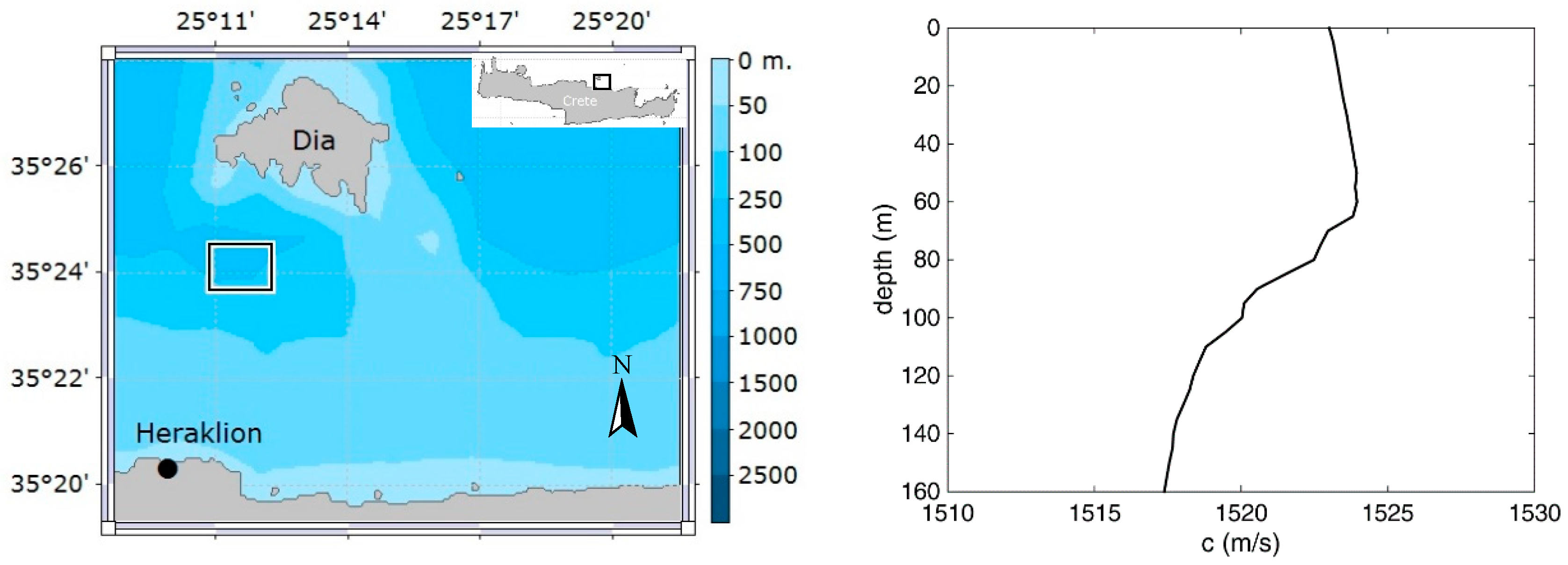
3.2.1. Experiment in Heraklion Bay
The first localization experiment was conducted on 15 December 2014 off the northern coast of Crete between the port of Heraklion and Dia Island, in an area with water depths between 140 and 180 m (
Figure 1). In this experiment the pinger was placed on the bottom—at a depth of ~160 m—in order to avoid bottom reflections that could possibly overlap with and degrade the surface-reflected signals. To check the readings of the array depth sensors used for the inversions, the TDR-2050 instruments were attached to the array next to the sensors.
Taking into account that the speed of sound is mainly influenced by temperature and pressure, whereas salinity has a secondary role, the sound speed profile during the experiment was derived from independent measurements of the temperature profile carried out with one of the TDR-2050 instruments before array deployment, using the Chen–Millero formula [
23] and assuming salinity equal to 39 ppt, a typical value for the eastern Mediterranean Sea. The sound speed profile is shown in the right panel of
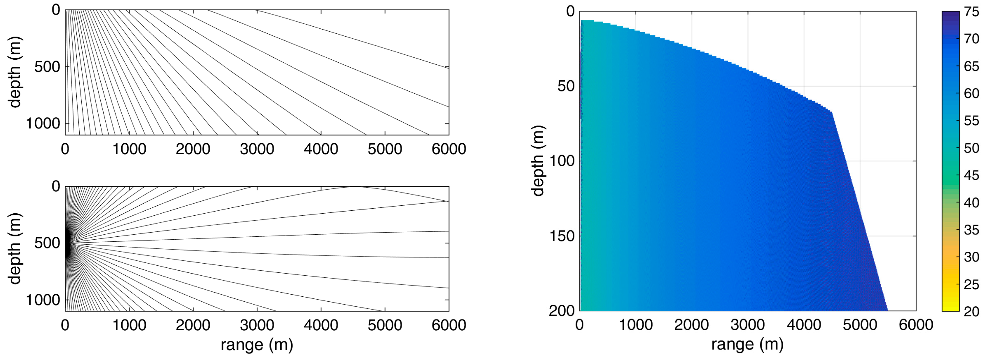
Figure 1. The sound speed has a maximum at about 60 m forming a surface duct which causes upward refraction and traps part of the acoustic energy close to the surface. Below 60 m the sound speed profile is downward refracting and bends acoustic rays towards the bottom.
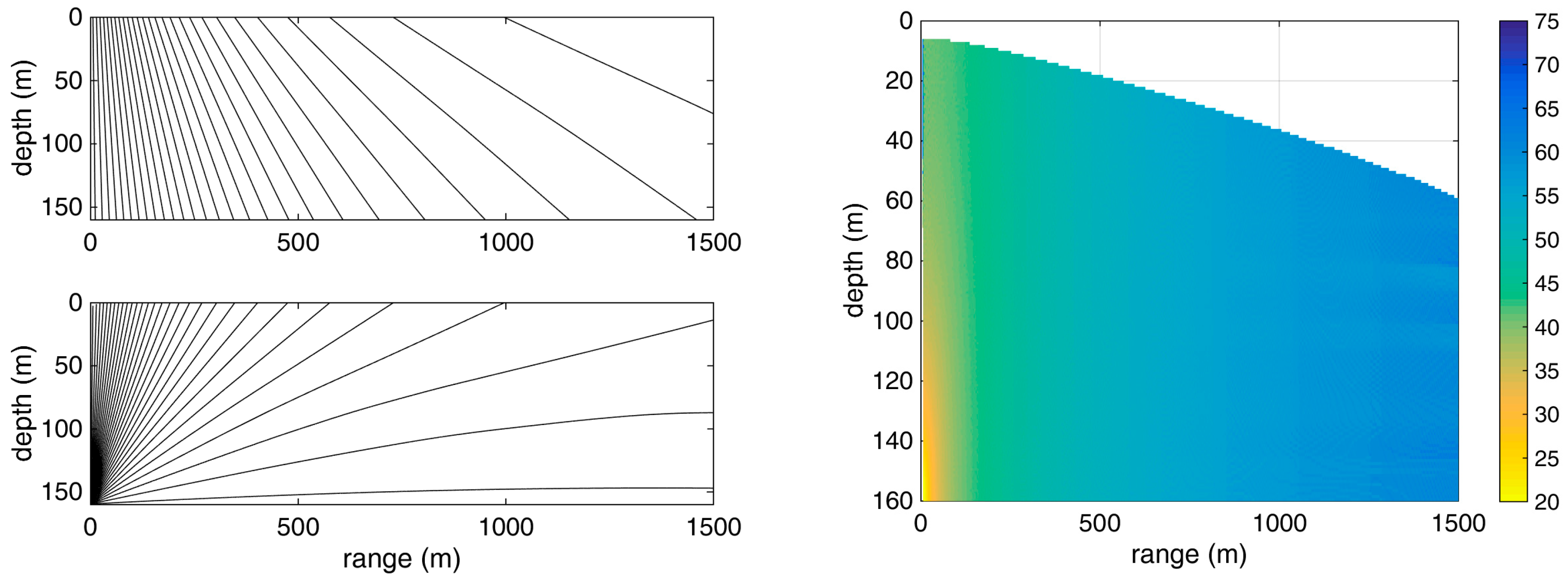
Figure 2 shows the predicted geometry of direct acoustic rays from a source at a depth of 160 m, as well as their surface-reflected continuation, in this environment. Both direct and surface-reflected rays provide a nearly homogeneous coverage. The graph on the right shows the area (in color) where the TDOA between direct and surface-reflected arrivals is larger than 7 ms, such that these arrivals are well separated in time. The longer the distance, the deeper the hydrophones have to be in order to avoid overlap between direct and surface-reflected arrivals, e.g., at a range of 1500 m the hydrophone has to be deeper than 60 m to receive distinct arrivals. The different colors denote the ray-theoretic transmission loss (TL) in dB according to the scale given on the right—in this calculation the frequency-dependent absorption was not taken into account such that the results are independent from frequency. From the figure, it can be seen that the TL closely follows the spherical spreading law [
24], whereas at ranges beyond ~1 km the effects of refraction in the form of weak ripples can be seen.
In the shallow-water experiment the hydrophone array was towed by a sailing boat (SV Maryline) running on engine at speeds of about 2 kn (~1 m/s). During the tow the hydrophones came close to the surface. At certain points stations were held to allow the hydrophones to sink to sufficient depths and provide well separated arrivals. At each station the engine, the echo sounder, and all electronic systems of the boat were switched off to minimize noise and interference.
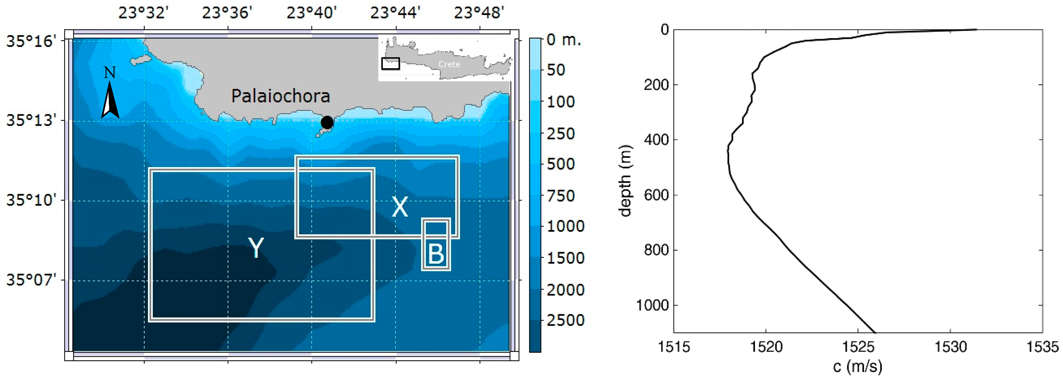
3.2.2. Deep-Water Experiment
The deep-water experiment was conducted in the period 6–8 June 2015 off Palaiochora, on the south coast of Crete (
Figure 3). On the first day of the experiment the pinger was deployed at 511 m depth in an area of 1500-m water depth and localization was carried out at distances up to 3 km from the pinger. On the following two days, pulsed signals (clicks) from two vocalizing sperm whales were detected, and the localization efforts focused on the animals.
In the deep-water experiment, the hydrophone array was towed by a fishing boat (FV Elena) and a number of stations were held to allow the hydrophones to sink and perform measurements. During these stations, the engine and the echo sounder of the boat were switched off.
The sound speed profile, as obtained from the temperature profile measured on 6 June by the RBR-Duo temperature-depth recorder, and the Chen–Millero formula assuming salinity of 39 ppt, is shown in the right panel of
Figure 3. It is a typical early summer sound speed profile for the area characterized by a strong thermocline in the upper 50 m followed by a milder negative gradient down to the axial depth of about 450 m. Below that depth the sound speed increases due to the effect of increasing pressure.
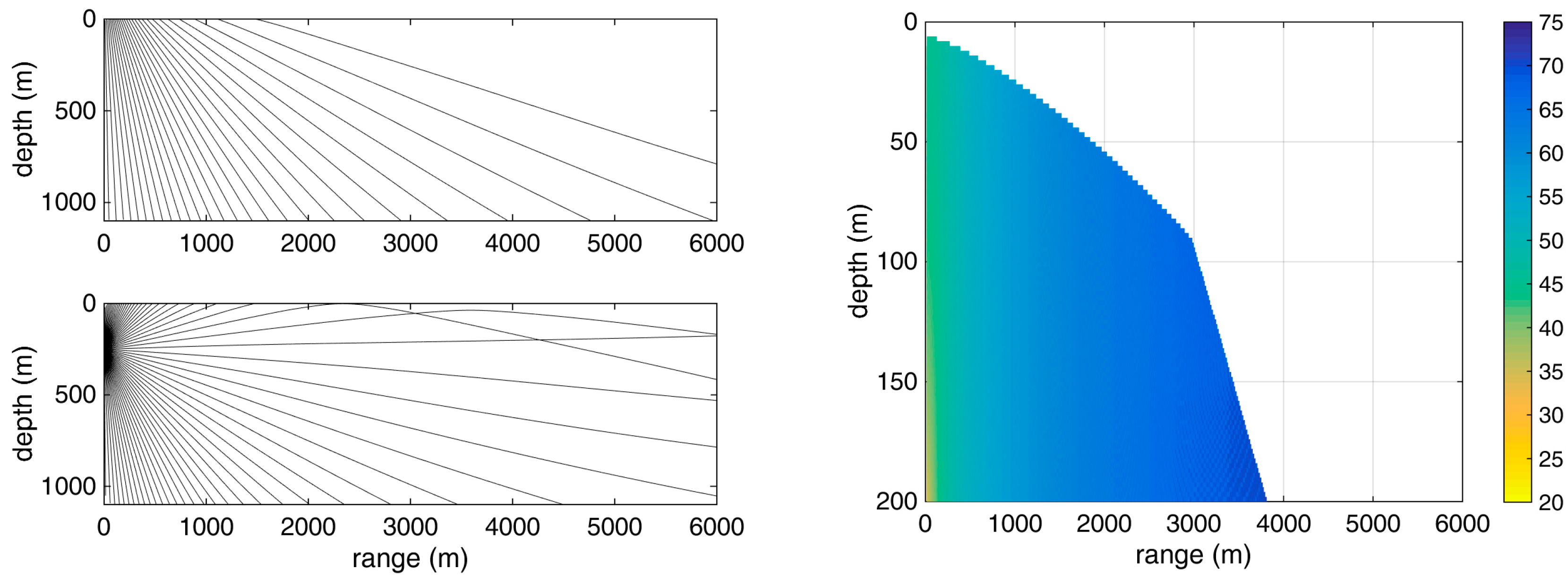
Figure 4 shows the predicted geometry of direct acoustic rays from a source at a depth of 250 m, as well as their surface-reflected continuation, in this environment. Refraction is evident at depths near the source depth, as well as close to the surface, especially beyond a range of ~2 km. Due to surface warming and associated increase of the sound speed towards the surface, downward refraction causes acoustic rays at ranges larger than 2 km to refract downward rather than reach the surface and be reflected. Because of this there are no reflections from the surface beyond ~2 km. The panel on the right of
Figure 4 focuses on the upper 200 m and shows the area (in color) where the TDOA between direct and surface-reflected arrivals is larger than 7 ms, whereas the colors denote the ray-theoretic transmission loss (TL) in dB according to the scale on the right. The longer the distance, the deeper the hydrophones must be to separate the direct and surface-reflected arrivals, e.g., at a range of 2 km the hydrophone must be deeper than 50 m to receive distinct direct and surface-reflected arrivals. For ranges longer than 3 km the boundary of the area is constrained not because of the time difference but because of lack of surface-reflected rays, as shown in the upper left panel; this causes a knee at the range of 3 km.
Figure 5 shows the predicted geometry of direct acoustic rays and their surface-reflected continuations for a deeper source located at 500 m depth. Refraction effects are weaker in this case due to the steeper angles in the near-surface layers. In this case, the range beyond which rays do not reach the surface increases to ~4 km. The panel on the right shows the area (in color) where the TDOA between direct and surface-reflected arrivals is larger than 7 ms; this condition can be fulfilled with hydrophones shallower than before, e.g., at a range of 2 km the hydrophones must be deeper than 25 m in order to resolve direct and surface-reflected arrivals. The knee in this case is formed at a longer range ~4.5 km due to the better coverage by surface-reflected rays. Again, the colors denote the ray-theoretic transmission loss (TL) in dB according to the scale on the right.
3.3. Analysis Software
A custom-made integrated software system was developed for the collection, registration, processing and analysis of the experimental data. The system was designed in such a way as to support both real-time field operations and a more detailed analysis of recorded data after the completion of experiments/measurements. It incorporates sound and environmental data processing and recording units as well as detection and localization codes in a user-friendly environment featuring a GUI/Control kernel and two distinct modules, the first for data acquisition and signal detection and the second for source location estimation.
The data acquisition and detection module is a two-stage processing module that collects and records the incoming flow of raw data (audio signals, hydrophone depths) and analyzes the audio streams by applying various filtering techniques (frequency bandpass filtering, energy filters, matched filters) to detect signals of interest for further processing. The location estimation and tracking module includes localization and tracking codes implementing the Bayesian estimation scheme described in the previous section.
The GUI/control kernel incorporates and controls the above modules and features separate modes of operation for both on-line real time tracking and off-line detailed data analysis. During localization at sea, the system is switched to the on-line operation mode to collect, record, and analyze streaming data from the various sensors (hydrophones, depth sensors, GPS) and produce tracking results displayed in near real-time on a geographical map. Alternatively, the system can be operated in off-line mode for the analysis of data from past localization experiments.
4. Localization Results
In this section, results from the shallow- and deep-water localization experiments off the north and south coast of Crete are presented. In the shallow-water experiment in the Bay of Heraklion the objective was localization of a pinger lying on the seabed at a depth of ~160 m. The deep-water experiment off Palaiochora in southern Crete started with localization of the pinger at a depth of 511 m and continued with localization of two vocalizing male sperm whales encountered in the area.
For the initialization of the iterative scheme in all localizations presented in the following, the standard guess for the initial values of source ranges
,
, and depth
rely on slant range and elevation angle estimates resulting from simple formulas based on the assumption of homogeneous medium [
16]. The initial values for the range/depth standard deviations are 200 m for the source ranges and 20 m/50 m for the source depth, for the shallow-water/deep-water experiment, respectively; in each iteration, these values are multiplied by 2.5 to finally relax the corresponding constraints. The localizations presented in the following are the results at convergence.
4.1. Shallow-Water Source Localization
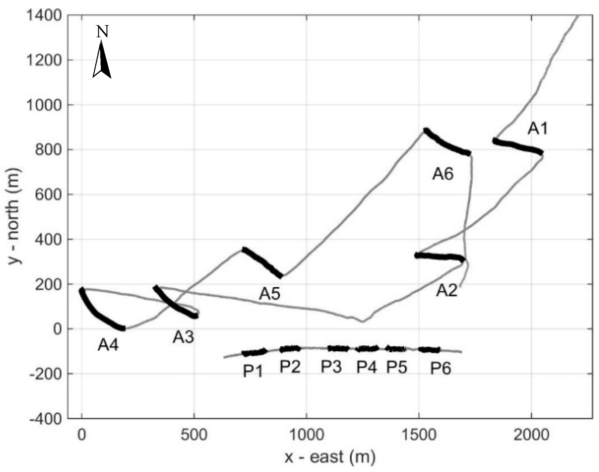
Figure 6 shows the track of the vessel towing the hydrophone array and also the track of the surface buoy from which the pinger was suspended during the shallow-water experiment on 15 December 2014. The experiment took place in an area with water depth between 140 and 180 m, with good weather and sea state between 1 and 2. The pinger was suspended at a depth of 160 m and was deployed in an area of about the same water depth (as measured by the boat echo sounder), such as to avoid bottom reflections. The vessel and the buoy/pinger locations during the experiment were tracked by the Astro GPS central and peripheral unit, respectively. After the deployment of the pinger the boat moved away and the hydrophone array was released to start the localization. Six stations were held, denoted by A1 to A6 in
Figure 6; the corresponding locations of the buoy attached to the pinger are marked by P1 to P6. It is seen that at each station there was a strong drift of the boat to the east/southeast, at a speed of ~1 kn (~0.5 m/s). Due to the strong current the buoy/pinger also drifted, approximately along the 160-m isobath, even though the pinger touched the bottom; traces of dragging (abrasions) as well as mud remains were observed on the pinger after its retrieval.
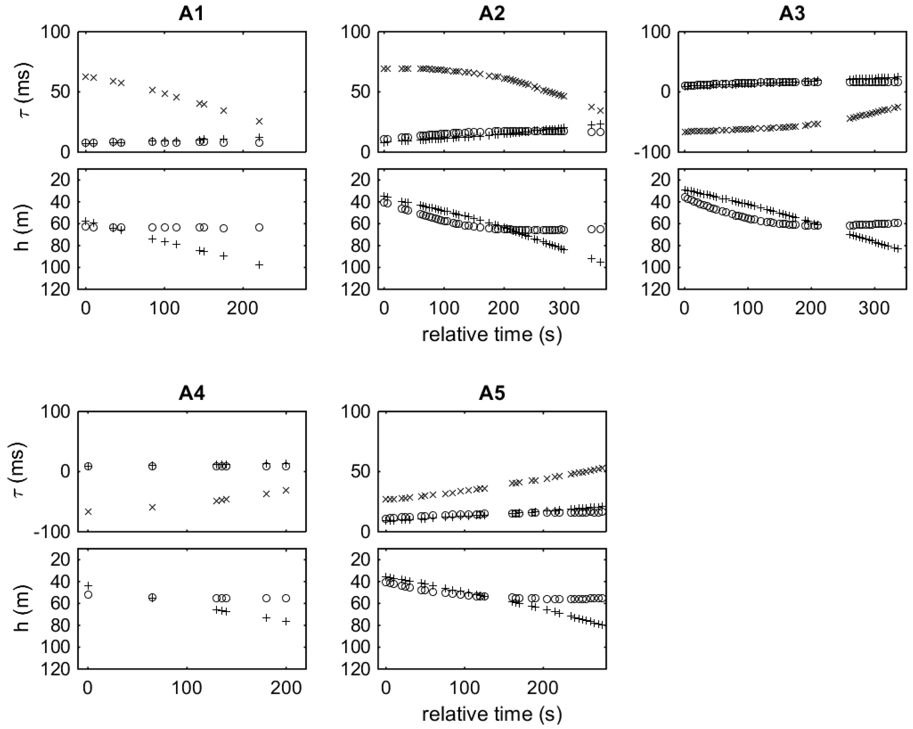
Figure 7 shows the TDOAs at the two hydrophones and hydrophone depths at stations A1 through A5. The acoustic signals at station A6 were of poor quality, mainly because of the presence of an approaching trawler (noise increase) but possibly also due to signal degradation caused by sinking of the pinger in mud or by the bottom topography around the pinger. The present localization approach is sensitive to SNR in two ways, in connection with both signal detection and travel-time estimation accuracy. Both detection capability and travel-time accuracy deteriorate with decreasing SNR, as described by the passive sonar equation [
25] and the Cramér–Rao lower bound [
25,
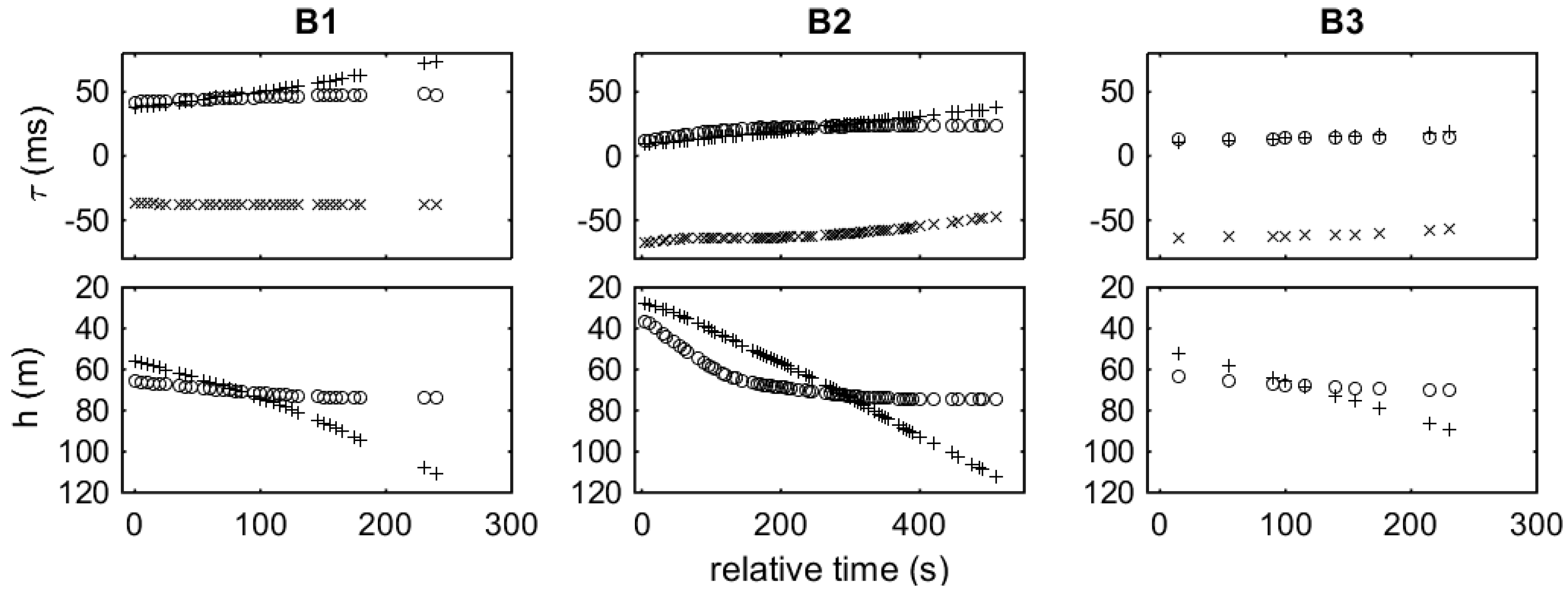
26], respectively. For signal detection and arrival time estimation bandpass filtering was used focusing on the frequency band between 10 and 12 kHz and, further, matched filtering (correlation with a replica of the emitted signal) was applied. For each reception, the TDOAs refer to the time difference between direct and surface-reflected arrivals—surface-reflected arrival time minus direct arrival time—for the front (circles) and rear (crosses) hydrophones, as well as the time differences between direct arrivals at the two hydrophones (x symbols)—arrival time at the rear hydrophone minus arrival time at the front hydrophone. The same symbols (circle for the front, cross for the rear hydrophone) are used for the hydrophone depths.
The maximum TDOAs between direct arrivals at the two hydrophones is related to the maximum distance (cable length) between the hydrophones, which is approximately 110 m. Therefore, the maximum time difference assuming sound speed ~1500 m/s is about 70 ms. As shown in
Figure 7, the TDOAs between direct arrivals are within the interval from −70 to +70 ms. Positive/negative values correspond to stations where the front/rear hydrophone is closer to the source, respectively. The TDOAs between direct arrivals at the two hydrophones generally change in the course of a station, reflecting changes in the orientation of the hydrophones relative to the source, as well as changes in the distance between the two hydrophones. In the course of the stations, the hydrophone depths increase with time—the hydrophones sink. This causes an increase in the difference between the lengths of the direct and surface-reflected paths, which reflects in the increase of the corresponding TDOAs.
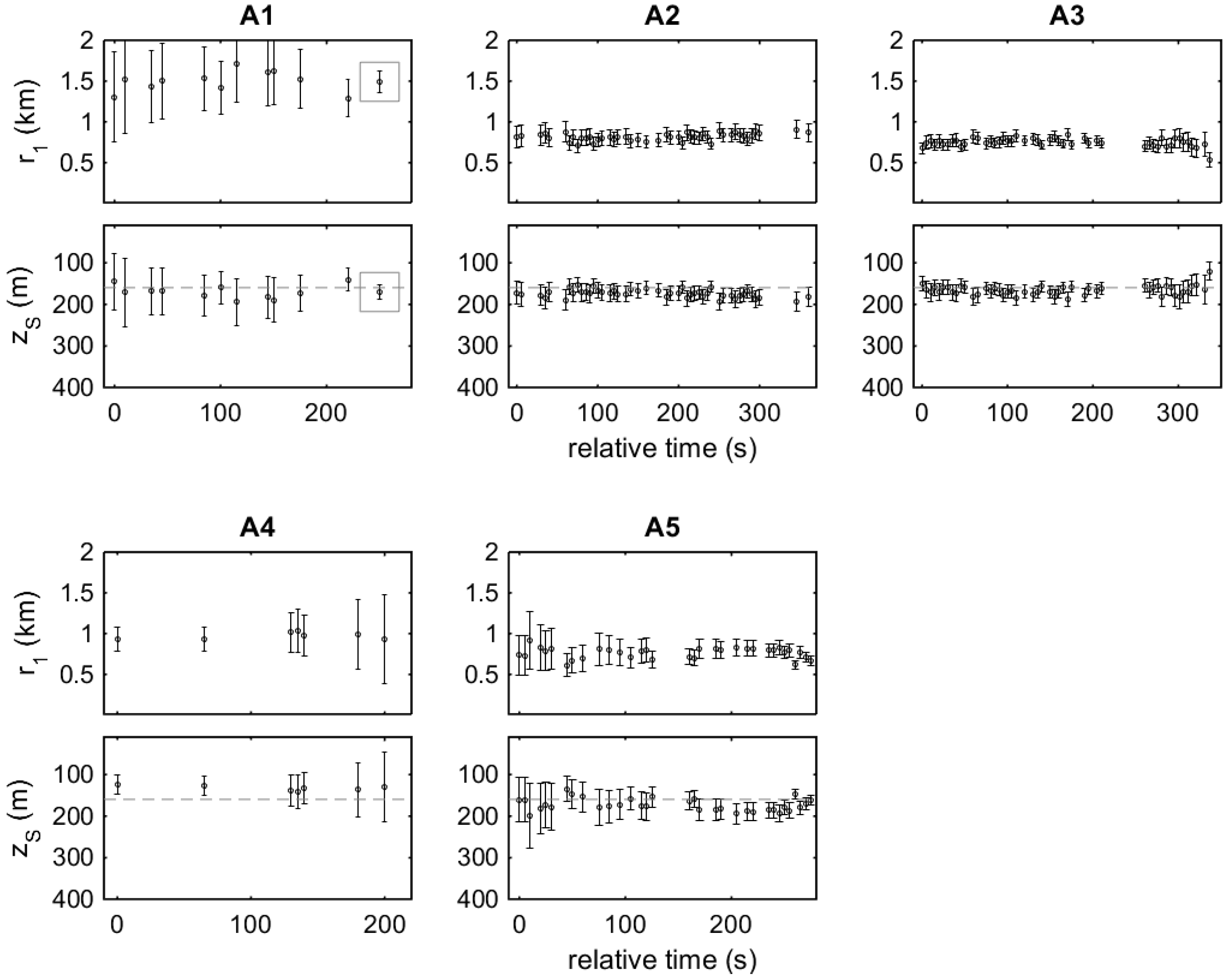
Figure 8 shows the results of range and depth estimation for stations A1 through A5 based on the data of
Figure 7 with errors of 0.1 ms RMS for the TDOAs and 0.2 m RMS for the hydrophone depths. Further, the sound speed profile shown in
Figure 1 was considered for propagation calculations, with an uncertainty which is maximum at the surface, where it has a standard deviation of 0.5 m/s RMS, and linearly decreases with depth up to 40 m, where it vanishes. The estimated means and error bars (posterior RMS errors) are shown in
Figure 8. The anticipated source depth of 160 m is also shown (dashed lines) to serve as ground truth. The horizontal locations of the source and the hydrophones, albeit close to the buoy and boat locations monitored by GPS, are not directly measured, and in this connection the anticipated range
is not shown in
Figure 8.
The estimated range at station A1 is around 1500 m with significant errors of ~500 m RMS. The large errors are attributed to the large distance to the source but also to the shallow depth of the source; the elevation angle (with respect to the horizontal) between the source and the hydrophones is close to 3.5°. When the source is at a small elevation angle, small changes in the TDOAs between direct and surface-reflected arrivals result in large changes in the direction of the range-depth locus leading to large uncertainties in the range and depth estimates. The estimated source depth is about 160 m, i.e., close to the anticipated source depth, but with large errors ~50 m RMS reflecting the same effect. The accuracy in this case can be significantly improved by averaging, as shown by the framed results in the A1 subplots corresponding to the average of the individual range/depth results—in that case, the mean of the average is the average of the individual means, whereas the covariance results from the average of the individual covariances divided by the size of the sample—thus, the RMS error of the average is smaller by a factor ~.
At station A2 the distance is about 850 m and the elevation angle has increased to about 7°. The errors for the range estimation are now ~100 m RMS and those for depth ~30 m. The fact that the pinger is close to endfire of the hydrophone array, as verified by the corresponding TDOAs between direct arrivals in
Figure 7, also contributes to the small errors. Station A3 gives a similar picture, but now the range is even smaller, about 750 m, and the source is in the wake of the towed array. The range errors in range are less than 50 m RMS and those in depth less than 20 m RMS, slightly increasing towards the end of the station. This error increase is attributed to the southeastward drift of the boat which towards the end of the station starts to pull the front hydrophone to the south thus changing the array orientation towards broadside with respect to the source, which gives rise in turn to larger errors. A similar situation with errors increasing with time appears in the case of station A4; nevertheless, the A4 data are of low quality due to increased level of background noise, such that only a few TDOAs could be estimated.
In the beginning of station A5, the boat and the array had an orientation from the southwest to the northeast such that the source is about 25° from broadside, which gives rise to the larger errors for the range and depth estimates in the beginning of the station. Then as the boat drifts to the southeast, it pulls upon the front hydrophone causing the array to turn in the clockwise direction and thus change its orientation with respect to the source toward the endfire, which in turn results in smaller errors in range and depth estimation. This is clearly seen in
Figure 8 A5, where the errors in range drop from ~250 m in the beginning of the station to less than 50 m RMS at the end, and where the errors in depth drop from ~50 m RMS in the beginning to less than 15 m RMS in the end, providing a close approximation to the anticipated source depth of 160 m.
4.2. Deep-Water Source Localization
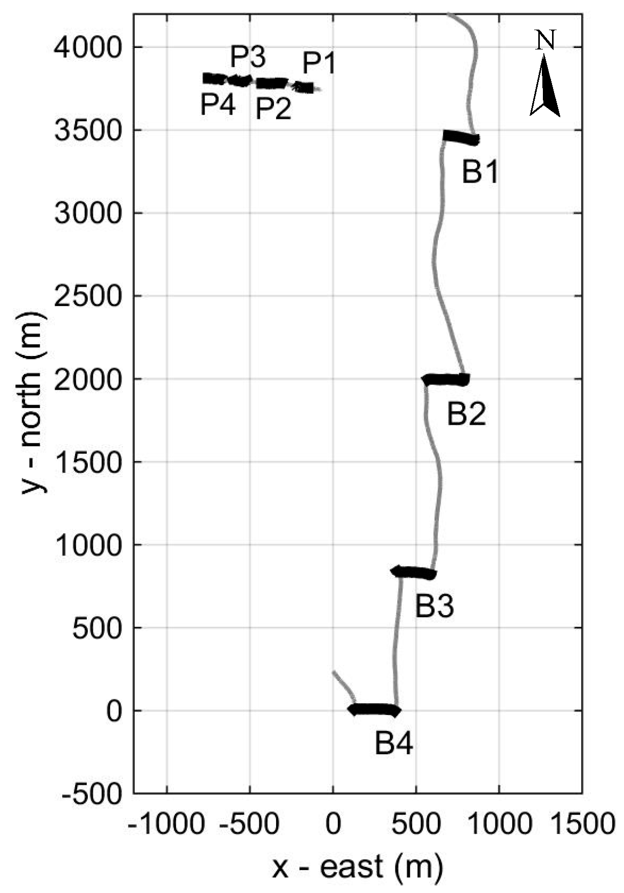
Figure 9 shows the track of the vessel and the buoy from which the pinger was suspended in the deep-water experiment on 6 June 2015. The experiment took place in an area with water depth exceeding 1500 m, in relatively good weather conditions and sea state between 2 and 3. After the deployment of the pinger at a depth of 511 m, four localization stations—B1 to B4—were held; the corresponding locations of the buoy/pinger are marked by P1 to P4, respectively. It is shown in
Figure 9 that there was a westward drift for the boat (clearly seen at the four stations where the engine was off) as well as for the buoy/pinger.
Figure 10 shows the TDOAs at the two hydrophones and also the hydrophone depths at stations B1 through B3. The pinger signals could hardly be detected at station B4 (at a distance of ~3.5 km). The limiting factor in that case turned out to be the high self-noise levels of the hydrophones, with equivalent input noise spectral density of 42 dB re 1 μPa
2/Hz, suggesting that the use of lower-noise hydrophones could enable localization at longer ranges.
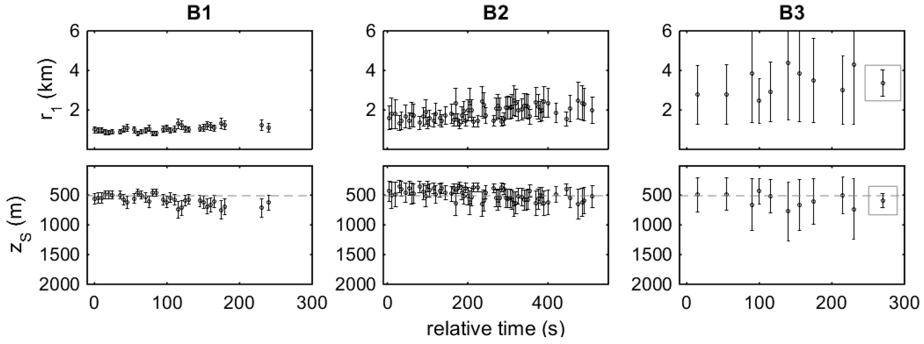
Figure 11 shows the results of range and depth estimation for stations B1 through B3 based on the data of
Figure 10 with errors of 0.1 ms RMS for the TDOAs between direct arrivals and 0.2 ms RMS for the TDOAs between direct and surface-reflected arrivals. These errors were obtained directly from the travel-time data after removal of systematic changes—the larger errors in
and
are assigned to the rougher sea surface. Further, an error of 0.2 m RMS was assumed for the hydrophone depths. The sound speed profile shown in
Figure 3 was considered for propagation calculations, with the same uncertainty as in the shallow-water experiment.
Figure 11 shows the estimated means and error bars (posterior RMS errors) for source range and depth, as well as the anticipated source depth of 511 m (dashed lines). The horizontal locations of the source and the hydrophones, albeit close to the buoy and boat locations monitored by GPS, are not directly measured, and in this connection the anticipated source range is not shown in
Figure 11.
The effect of sea surface roughness on two-hydrophone localization has been considered in [
17]. In addition to a reduction in signal coherence and signal level of the surface-reflected arrivals due to scattering, large-scale roughness affects the corresponding arrival times and the induced RMS error is proportional to the sea surface RMS roughness
and the sine of the grazing angle
[
27]
where
is a typical sound speed value (1500 m/s). In the localization experiments the grazing angle varied typically between 10° and 25°. Sea states 2 and 3 are characterized by significant wave heights up to ~0.4 m and up to ~1.2 m, respectively, corresponding to sea surface RMS roughness values ~0.1 m and ~0.3 m [
28]. Taking an average value of ~17° for the grazing angle
and a typical sound speed value of 1500 m/s the above expression gives 0.04 ms for sea state 2 and 0.12 ms for sea state 3. In the shallow water experiment, the TDOAs errors were set to 0.1 ms, larger than the above estimate for sea state 2, which indicates that surface roughness induced errors were small and negligible in that case. On the other hand, in the deep water experiments, with sea state close to 3, the estimated error becomes significant and contributes to an overall error increase in the TDOAs between direct and surface-reflected arrivals, justifying the larger error values (0.2 ms) in the deep-water localizations.
The station B1 is at a range ~1000 m from the source with the array having a north–northeast orientation. This is verified by the TDOAs between direct arrivals at the two hydrophones of ~0.4 ms which for a distance of ~100 m between the hydrophones suggests a deviation of ~50° from endfire. The range estimates at station B1 are around 1 km with errors ~150 m RMS. The depth estimates are about 550 m, which is close to the actual pinger depth (dashed line), with errors ~75 m RMS. The latter are proportionally larger than those resulting from the shallow-water experiment. This has to do with the higher elevation angle of the source close to 30° which for the same error in range estimation results in a larger depth error. It is seen from
Figure 11 that the errors increase slightly towards the end of station B1. This is caused by the westward drift of the boat which changes the orientation of the hydrophone array in the clockwise direction such that the source/pinger gets closer to broadside where the errors are larger.
At station B2, the range increases to ~2 km and the estimation errors increase accordingly. The azimuthal position of the source is now closer to endfire, as indicated by the larger values of the TDOAs between direct arrivals at the two hydrophones in
Figure 10. The errors in range estimation are ~500 m RMS and in depth estimation about 200 m RMS about the true source depth. Again, there is a slight error increase with time, which is attributed to the drift of the boat and the turn of the array (away from endfire).
At station B3, the range increases to ~3 km and the errors of individual inversions are of the order of 1000 m RMS or even larger, again increasing toward the end of the station. Similarly, the errors in depth estimation are significant, ~300 m RMS or higher, increasing toward the end of the station as well. Even though the individual localization results may be of limited use because of the large errors, the situation can be improved by averaging. The framed localization results in the B3 subplot correspond to the averages of the individual range/depth estimates.
4.3. Localization of Sperm Whales
Two different solitary male sperm whales, named here for convenience as whale X and Y, were encountered on 7 and 8 June 2015, respectively, and offered the opportunity for an alternative application and testing of the localization method. Sperm whales spend most of their time diving to depths of several hundred meters in search of food, mainly mesopelagic and bathypelagic cephalopods (squid). During each dive, which may last up to one hour, the animals rely exclusively on sound for communication, navigation, surveillance and foraging. Their most typical sounds are the so-called regular clicks, long sequences of broadband pulsed sounds of ~5 ms duration, with repetition periods of the order of 1 s [
29,
30]. In the following, localization results for the two whales are presented based on the analysis of click receptions at the two hydrophones. For the real-time localization carried out in the field, energy filters (moving average of the squared acoustic pressure with averaging window of 2.5 ms) were used to estimate click arrival times.
Figure 12 shows an extract from a sequence of regular clicks from one of the whales and a detailed view of a single click. The double arrivals in the click sequence correspond to direct and surface-reflected paths, with the direct arrivals arriving first.
The only way to verify the localization results in the case of sperm whales was to witness surfacing of the animals. To achieve this, localization of the animals also in the horizontal was necessary, which in turn required knowledge about the horizontal location of the two hydrophones. To obtain an estimate for the horizontal location of the hydrophones during the tow and also during stations a simple model for the array geometry was used, taking into account the hydrophone depths and the boat track and also accounting for the distance between hydrophones based on cable lengths. According to the model used, as the boat sails or drifts the front hydrophone is allowed to move only in the forward direction along the straight line to the new boat location. This approach was incorporated in the real-time analysis system used in the field, which enabled horizontal localization of the animals in addition to depth/range estimation. Thus, position estimates on a map were available, subject to left–right ambiguity, of course, which in some cases was resolved by changing the array orientation, through drifting and/or maneuvering. When there was indication about dive completion (e.g., end of click sounds taking into account dive duration) the boat tried to move towards the last estimated position in order to witness surfacing. The results are presented in the following.
4.3.1. Sperm Whale X
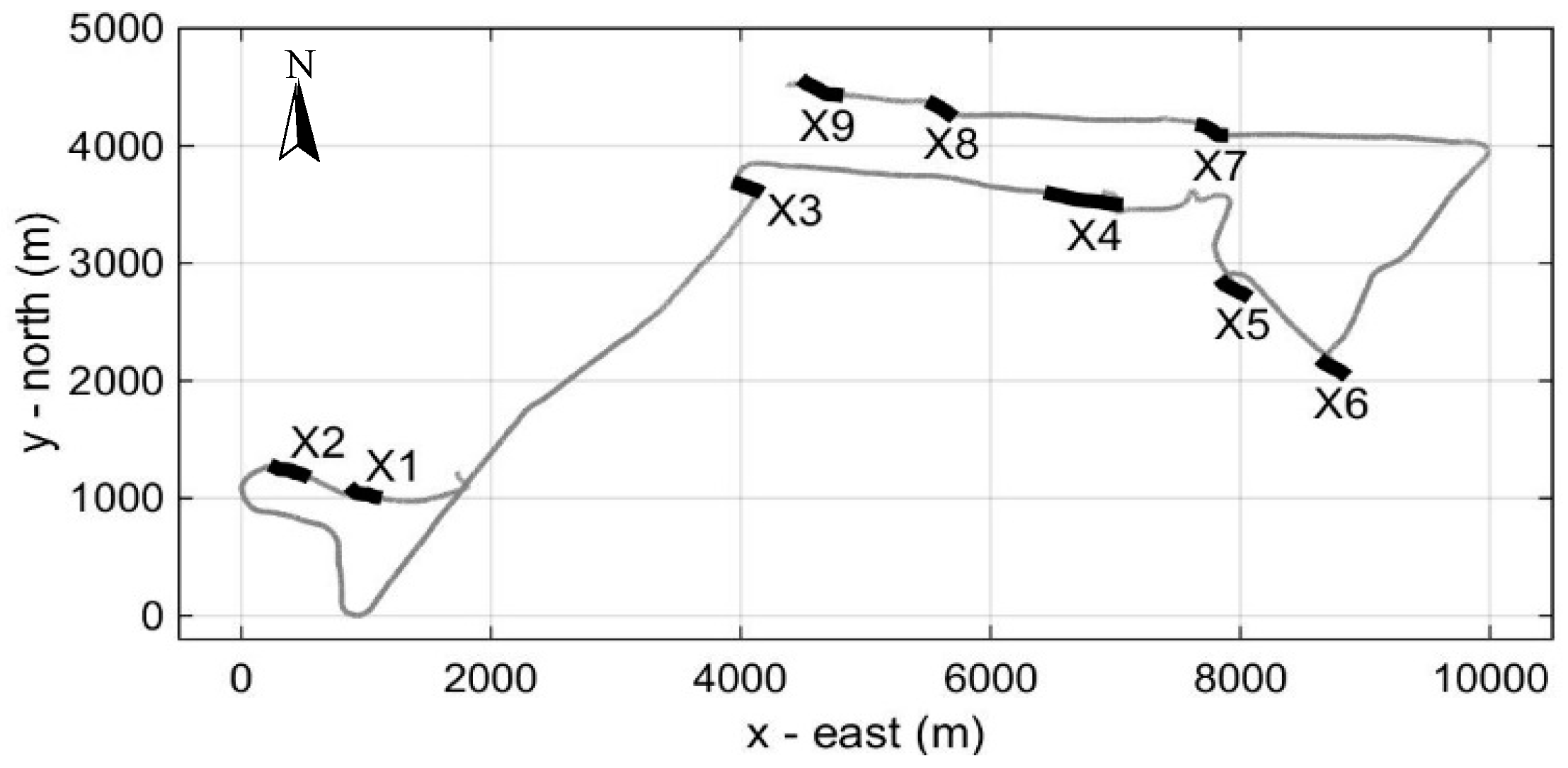
Figure 13 shows the course of the vessel on 7 June 2015 aiming at the localization of sperm whale X. The weather was fairly good and the sea state around 3. A total of nine stations, X1 to X9, were performed (
Figure 13). After station X2 the whale surfaced but was not visually detected due to long distance. The next surfacing took place after station X4 and was visually witnessed—the whale was followed while at the surface. Another surfacing took place after station X6 and it was visually witnessed as well—again the whale was followed while at the surface. After the start of the next dive, the vessel changed course to the west and performed the last three stations, X7 to X9.
Figure 14 shows the TDOAs at the two hydrophones and hydrophone depths at stations X2 through X7. At station X1 the data are similar to those at station X2 and are not shown. At stations X8 and X9, the signal quality was too low for travel-time estimation and localization.
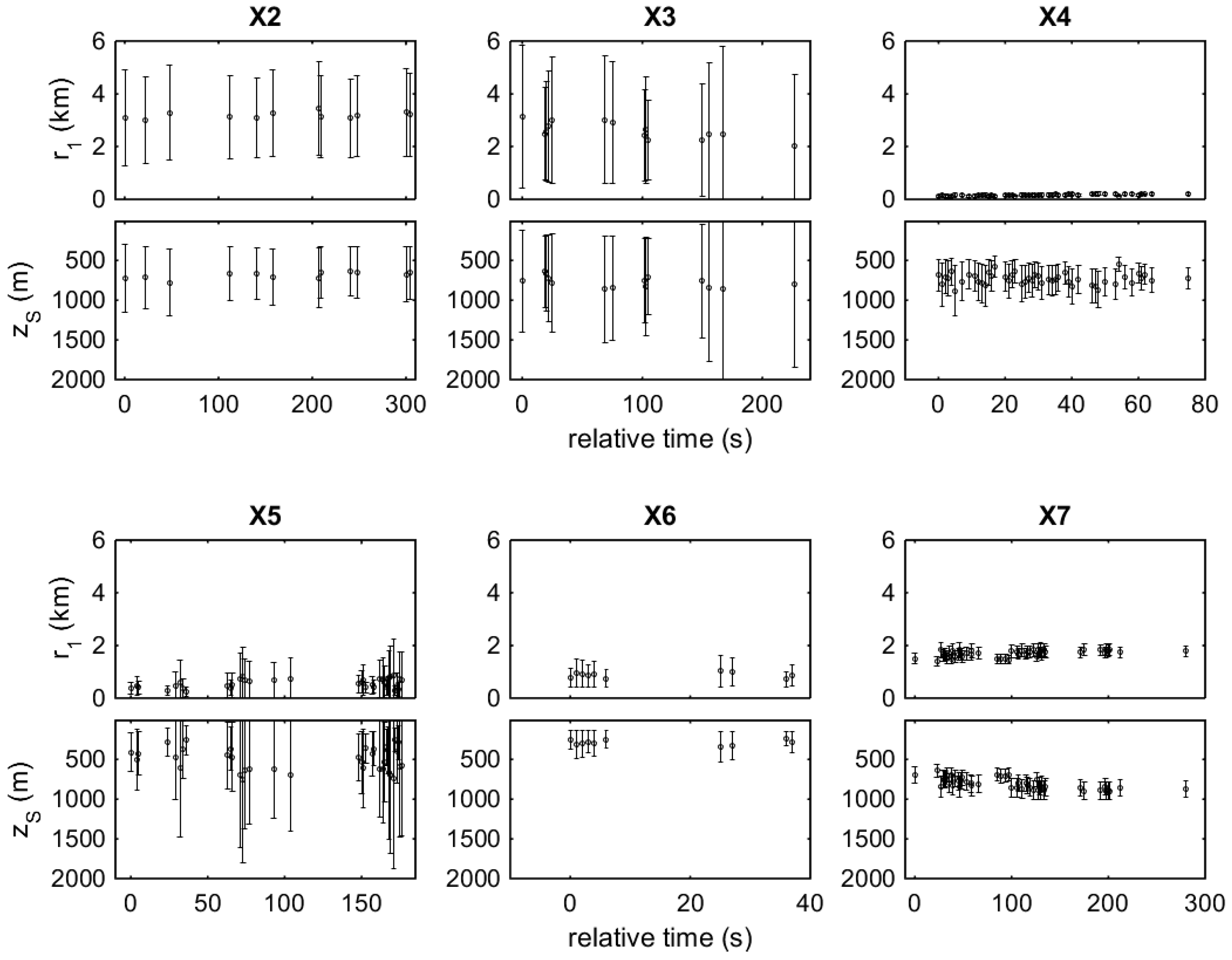
Figure 15 shows the results of range and depth estimation for stations X2 through X7 based on the data of
Figure 14 with errors of 0.1 ms RMS for the TDOAs between direct arrivals, 0.2 ms RMS for the TDOAs between direct and surface-reflected arrivals, and 0.2 m RMS for the hydrophone depths. Further, the sound speed profile shown in
Figure 3 was considered for propagation calculations, subject to the same uncertainty as before.
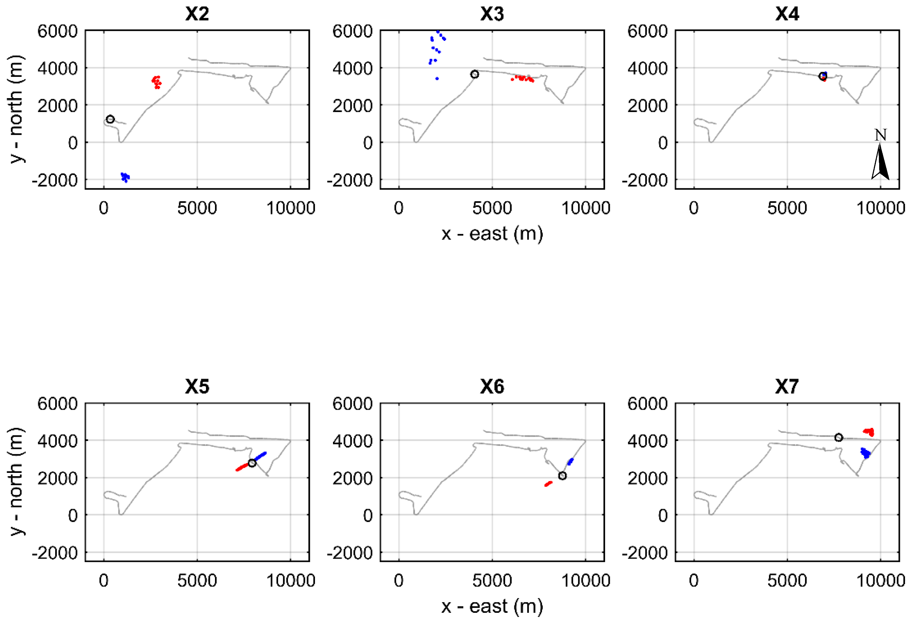
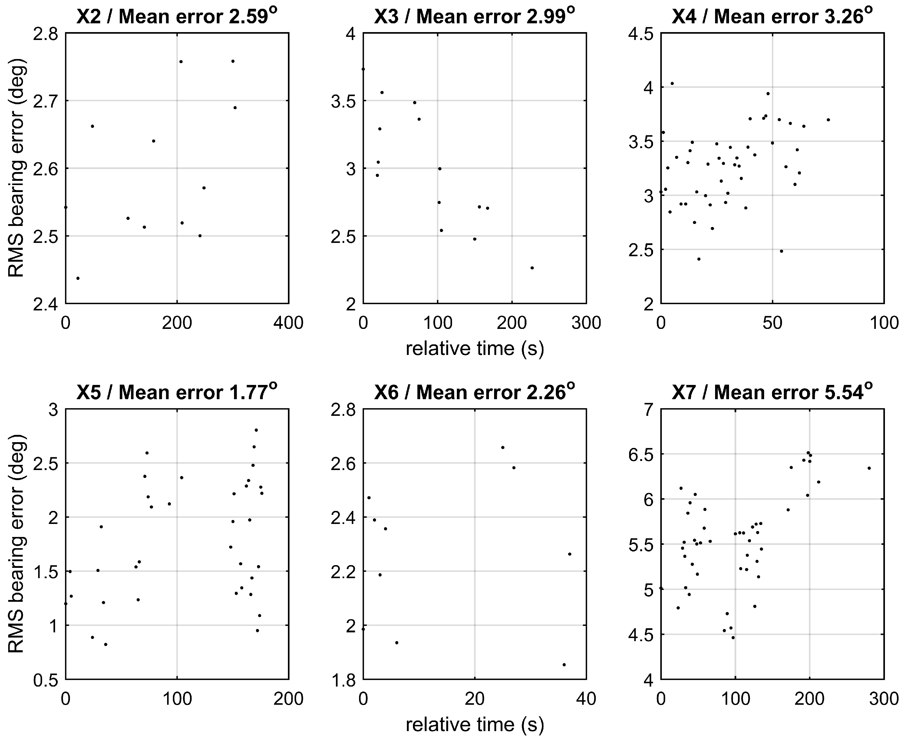
Figure 16 shows the estimated horizontal positions of whale X at stations X2 to X7 while
Figure 17 shows the corresponding errors in estimating the azimuthal angle at each station using the simple bearing estimation approach [
5]. In each panel of
Figure 16, the position of the vessel in the middle of the station is marked by a circle superposed on the vessel track. The localization in the horizontal is subject to left–right ambiguity. The two symmetrical solutions with respect to the vertical plane through the two hydrophones are marked by the different colors. It is noted that the RMS errors shown in
Figure 15 and
Figure 17 are statistical errors describing the uncertainty of the localization results, not actual errors i.e., differences between estimated and true whale locations which are unknown.
At station X2, the first localizations resulted in range estimates between 3 and 3.5 km subject to significant errors ~1.5 km RMS and depths of about 600 m with errors ~400 m RMS. The horizontal localization gives two families of solutions in
Figure 16, symmetrical with respect to the hydrophone array and separated by ~6 km. Shortly after station X2, it had to be decided which one of the two families to select without any further information, the northern family was selected based on biological reasoning since it was closer to the coast and in a shallower area of ~1000 m water depth where sperm whales usually feed, whereas the solutions in the south were in a much deeper area (~3000 m). The bearing estimation errors are relatively small, around 2.6° RMS, due to the source azimuth orientation being close to broadside.
Station X3 resulted in a range estimate about 2.5–3 km and a depth about 750 m subject to large errors ~2 km RMS and ~500 m RMS, respectively, pointing to orientation close to broadside. This is confirmed by the small values in the TDOAs between direct arrivals in
Figure 14, decreasing from 30 to 0 and further to −10 ms associated with the westward drift of the vessel while at station. Since the vessel enters station X3 from the southwest, this points to location of the source on the east, such that initially the front hydrophone is closer, and then as the vessel drifts to the west the array turns counterclockwise, passes through broadside, and keeps turning such that finally the rear hydrophone is closer to the source. Orientation close to broadside leads to large errors in range/depth estimation, as seen in
Figure 15, and small errors in bearing estimation. The results in
Figure 16 confirm the near-broadside orientation; interestingly, the two symmetric solutions exhibit quite different character in this case: while the solutions on the east are very concentrated azimuthally, the solutions on the west are highly dispersed. This is attributed to the changing orientation of the hydrophone array and offers a criterion for the selection of the correct solution—the one on the east with the minimum spread—while at the same time, it verifies the model used for the array geometry.
The results at station X4 indicate that the whale is very close, just 150 m from the front hydrophone in the horizontal, with errors ~60 m RMS, still quite deep at about 750 m estimated depth with error ~250 m RMS, decreasing as the rear hydrophone sinks. After station X4 the sperm whale ascended to the surface and was visually observed for the first time. During the surfacing which lasted for ~10 min the whale followed a course to the east, and the boat followed the same course just behind and slightly to the side of the whale.
After the start of the next dive the boat moved in a steady diverging course of about 45° from the assumed course of the whale and two stations, X5 and X6, were held. The fact that the source is on the side of the array, especially at station X5, is confirmed by the very small TDOAs between direct arrivals in
Figure 14, leading to large errors in distance and depth estimation and small errors in azimuthal angle. This is seen in
Figure 15 for X5, where the estimated values for both range and depth are about 500 m with errors of similar magnitude on average, whereas the average error in bearing estimation is less than 2° RMS. Even a slight departure from broadside at X6 reduces the errors in distance and depth estimation. Thus, at station X6 the distance is estimated at about 1000 m with an error ~500 m RMS and the depth at about 250 m with an error ~200 m RMS. The anticipated stability in bearing estimation is seen in
Figure 16 and
Figure 17; despite the great variation in distances, the azimuthal position is remarkably stable for both stations.
After station X6, the whale surfaced for ~5 min as was visually observed for the second time. While at the surface the whale followed a course to the northeast. During the surfacing the boat remained just behind and slightly to the side of the whale. Immediately after the start of the next dive, the boat turned and followed a westward course and shortly after station X7 was held, aiming at an endfire orientation of the whale with respect to the hydrophone array to provide relatively small range/depth errors. The estimated range in
Figure 15 is about 1.6 km with an error ~200 m RMS. The endfire orientation is confirmed by the TDOA between the direct arrivals,
Figure 14, which is greater than 60 ms (near the maximum possible value of 70 ms), but also from the localization in the horizontal,
Figure 16. The bearing estimation errors for X7,
Figure 17, are ~5.5° RMS, and are larger than those at other stations.
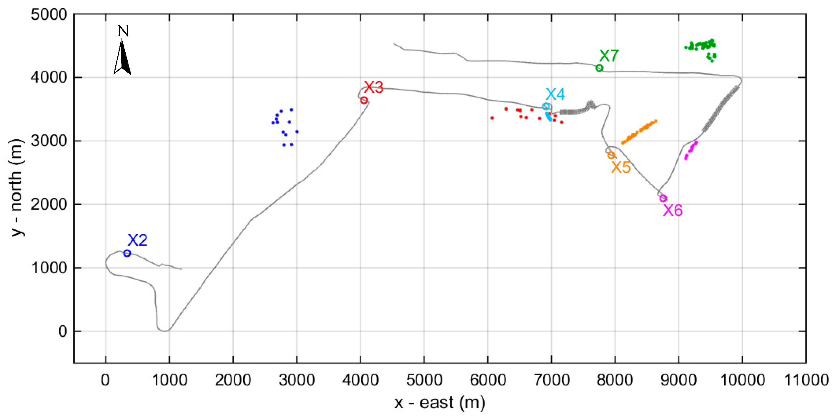
In
Figure 18, the horizontal localization results from the various stations are combined after selecting one of the two symmetrical solutions for each case. The criteria used for this selection were the minimum horizontal spread and the consistency with the remaining predictions (localization from the other stations). The vessel track is also shown in this figure by consecutive thick grey dots during visual observation, when the vessel track coincides with that of the whale. The vessel location in the middle of each station is marked by a circle of different color—the same color is used for the corresponding localization results (dots).
From
Figure 18, it is seen that the whale initially moves in the eastward direction. After station X2, another station was about to be held with a different orientation in order to resolve left–right ambiguity—this is why shortly after station X2 the boat changed its course to the south—but then the whale stopped clicking and ascended to the surface, so instead of holding a station the boat moved to the northeast, to the position estimated at station X2 (selecting the more reasonable one from the two families of solutions from the biological point of view—the one closer to the 1000-m isobath) but did not manage to reach the surfacing area in time due to the large distance. Then station X3 was held and resulted in a horizontal estimated range of about 3 km to the east (the left–right ambiguity in this case was resolved using the different angular spread as described above). The boat moved to the estimated position and performed station X4 which confirmed the X3 estimate and resulted in very short estimated ranges. The whale then ascended to the surface where it remained for ~10 min and was visually observed for the first time. During the surfacing, the boat (grey dots) followed the whale.
After the start of the next dive, the boat moved in a steadily diverging course of about 45° from the assumed course of the whale and held stations X5 and X6 that resulted in localizations on the extension of the whale course to the east, albeit subject to large range errors due to broadside orientation. The whale then emerged again for 5 min and was visually observed for the second time. Again during surfacing, the boat followed the whale (heavy line). It is of interest here that this course is no longer to the east but to the northeast. Then, immediately after the start of the next dive, the boat turned and moved west. Localization at station X7 results in position estimates lying northwest of the point where the whale left the surface. This result, considered in combination with the northeastern course of the animal during the previous surfacing, indicates that the whale might have changed its eastward course and turned to the west.
4.3.2. Sperm Whale Y
In the morning of the following day, 8 June 2015, faint clicks from another sperm whale, named here as ‘whale Y’, were detected outside the port of Palaiochora, indicating that the animal was at a large distance.
Figure 19 shows the course of the vessel for the localization of whale Y, which now spans a much larger area than on the previous day. The weather conditions and sea state were about the same. A total of 20 stations, Y1 to Y20, were held. Useful data for localization are available at seven stations: Y8, Y10, Y11, and Y14 to Y17; at the remaining stations either the signal was of low quality due to large distance or there were no vocalizations at all. The whale was first sighted after station Y9, albeit with a delay and at a distance. A second witnessed emergence occurred after station Y11, after which the boat followed the whale. The third surfacing took place after station Y16 and it was again visually witnessed. In this third emergence, the whale spent a long time at the surface moving southeast and was followed up to a point where the boat changed its course to the northeast. Then, while at a distance, the whale was seen diving and shortly after the start of regular clicks station Y17 was held.
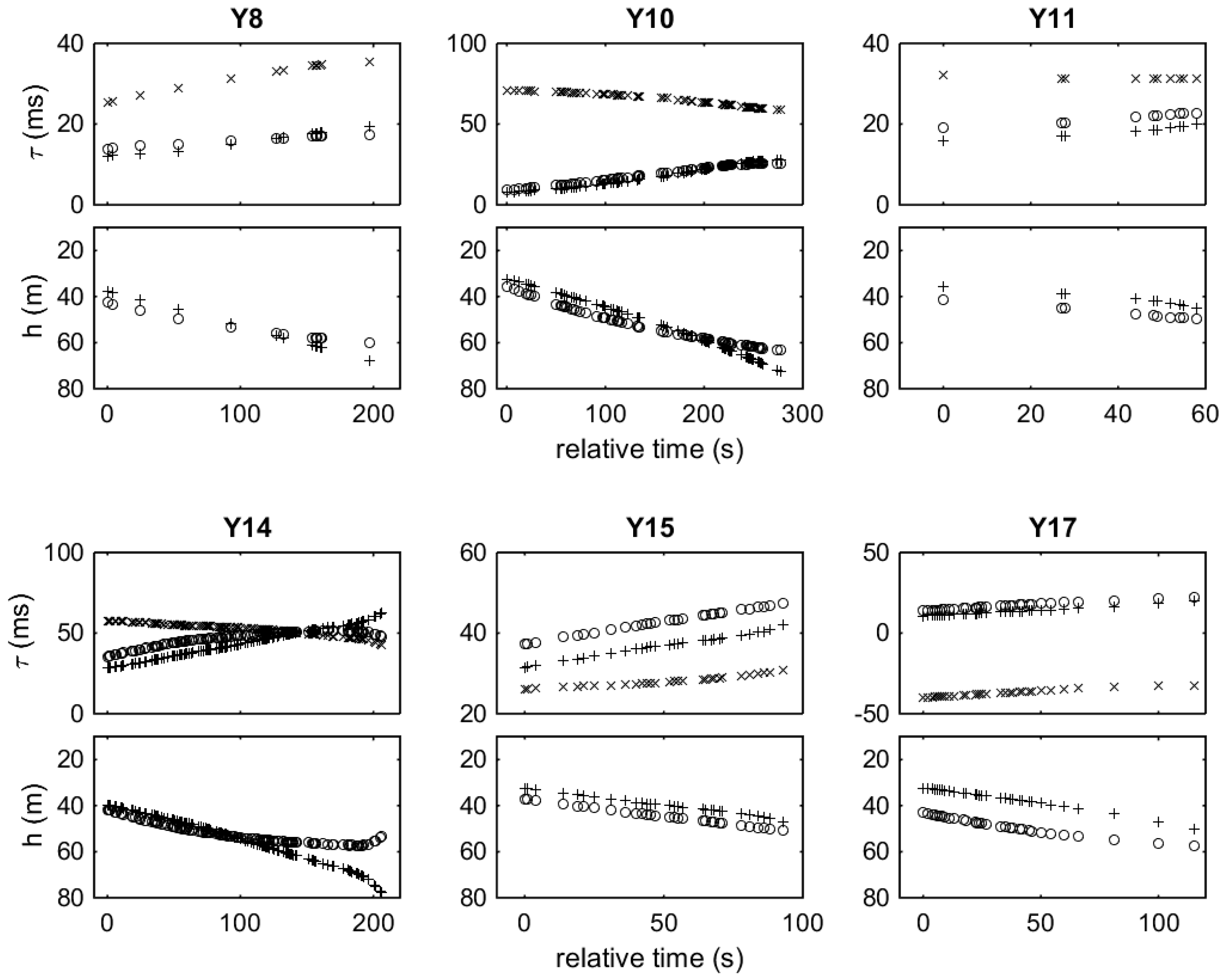
Figure 20 shows the TDOAs and hydrophone depths during stations Y8, Y10, Y11, Y14, Y15, and Y17. Station Y16 is not included because of highly uncertain orientation of the hydrophones due to the abrupt change of the vessel course after station Y15.
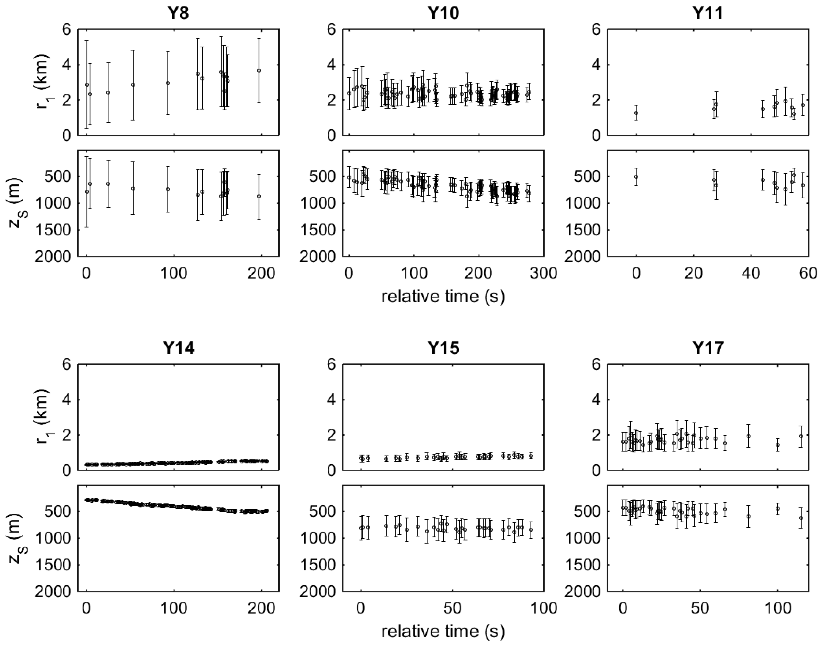
Figure 21 shows the corresponding range and depth estimates assuming the same errors and uncertainties as in the previous case of whale X.
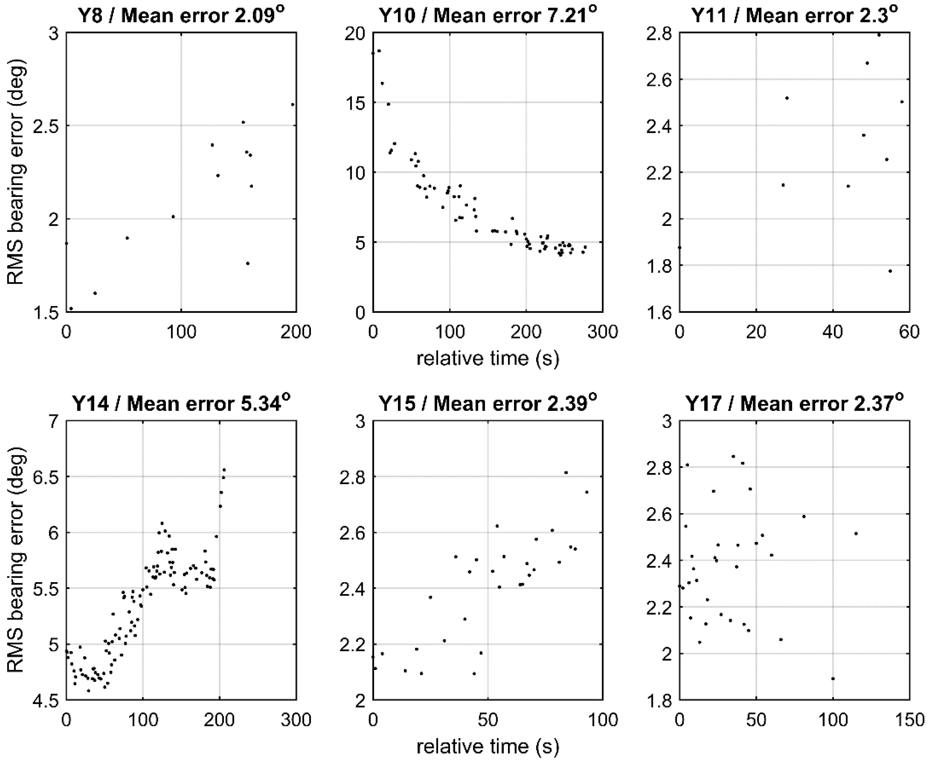
Figure 22 shows the estimated horizontal positions while
Figure 23 shows the corresponding errors in bearing estimation. As mentioned before, the RMS errors shown in
Figure 21 and
Figure 23 are statistical errors describing the uncertainty of the localization results, not actual errors—i.e., differences between estimated and true whale locations which are unknown.
The first localizations at station Y8 result in range estimates of about 3 km with errors ~2 km RMS and depth estimates of about 700 m with errors ~500 m RMS. The large errors are due to near-broadside orientation of the array relative to the vocalizing animal, as confirmed by the relatively small TDOAs between direct arrivals in
Figure 20, and also by the horizontal localization results in
Figure 22, in which case the two solution families and the vessel (apex) form an angle close to 160–170°. Noteworthy are also the small bearing estimation errors, about 2.1° RMS, in
Figure 23, in accordance with theoretical predictions. Further, it is seen in
Figure 22 that from the two families of solutions the southern one is concentrated in the azimuth while the one in the north is more dispersed, apparently due to a change in the orientation of the hydrophones in the course of the section, a fact which suggests that the southern solution is the correct one.
At the beginning of station Y9, the whale stopped clicking and ascended to the surface. The boat moved to the south (towards the estimated location area from station Y8) and the whale was sighted while at the surface, albeit with a delay and at a long distance, and started his next dive before the boat could come close. The next station Y10 took place during this dive and resulted in range estimates about 2.5 km subject to errors ~800 m RMS and depth estimates increasing from 500 to 800 m, which corresponds to a typical dive profile, with errors ~150 m RMS decreasing in the course of the station as the hydrophones gradually sink. It is noted here that clicks also exist at shallower depths, but due to the long distance of the whale and the shallow hydrophone depths direct and surface-reflected arrivals overlap with each other, cf.
Figure 4.
Taking into account the large values in the TDOAs between direct arrivals in
Figure 20 at station Y10, close to +70 ms, the whale is close to endfire and closer to the front hydrophone, i.e., the whale is in front of the boat. This explains the much smaller errors in range and depth estimation, compared to station Y8 where the orientation was close to broadside. The endfire orientation is confirmed by the horizontal localization results in
Figure 22, where the two families of solutions exhibit a different degree of concentration in the azimuth, apparently due to a change in the hydrophone orientation, with the more concentrated solutions (the ones to the east) being more likely to be correct, as is also confirmed in the following. The change in the hydrophone orientation away from endfire in the course of the station Y10 leads to a significant reduction in the azimuth angle estimation error, as confirmed by the results in
Figure 23, where azimuth angle estimation errors drop from 15° to 5° RMS in the course of the station.
Immediately after station Y10, the boat changed its course following a different direction and after a while held station Y11 in order to resolve the left–right ambiguity of section Y10. Station Y11 results in range estimates of about 1.6 km with error ~600 m RMS and depth estimates of about 700 m with error 200–300 m RMS. The relatively large range and depth estimation errors are due to the array being closer to broadside orientation, as verified by the smaller TDOA values between direct arrivals in
Figure 20, compared to those at station Y10, and also by the horizontal localization in
Figure 22, and leading also to smaller errors in bearing estimation about 2.3° RMS, as shown in
Figure 23. Regarding the selection from the two families of horizontal locations estimated from stations Y10 and Y11, it is seen in
Figure 22 that the eastern ones are in agreement with each other whereas the western ones are not. After station Y11 the whale emerged and stayed at the surface, or close to the surface, for a long time, about 30 min. During this time the animal was visually observed and followed by the boat. Stations Y12 and Y13 took place during that period when the whale performed a shallow dive close to the surface but produced no clicks. Then the whale reemerged and stayed at the surface for more than 10 min and finally started a normal dive. At the beginning of this dive, as soon as the whale started clicking, the next station, Y14, was held.
Station Y14 results in range estimates increasing from 400 to 600 m with an error ~50 m RMS and depth estimates increasing from 250 to 500 m with error about 10 m RMS, describing a dive profile with the whale descending at a rate of about 80 m/min. The small errors in range and depth estimation are due to the small distance, but also due to the orientation of the whale in front of the boat (endfire) while diving away. On the other hand, this gives rise to larger errors in bearing estimation ~5.3° RMS, as seen in
Figure 23.
After station Y14, the boat followed a course of slightly different direction from the anticipated whale course and held the next station, Y15, performing a similar maneuver as in the case of stations Y10 and Y11. Station Y15 results in range estimates of about 750 m, slightly increasing, with error ~200 m RMS and depth estimates about 800 m with error ~200 m RMS. The larger errors are due to the deviation from the endfire orientation, as confirmed by the smaller TDOA values between direct arrivals in
Figure 20 and also by the horizontal localization results in
Figure 22, resulting in smaller bearing errors, about 2.4° RMS, in
Figure 23. Station 15 was interrupted because the whale stopped clicking, but shortly afterwards it started clicking again and station Y16 was held but was also interrupted since the whale finally ceased clicking and ascended to the surface where it remained for about 50 minutes. While at the sea surface, the whale moved southeast and was followed up to a point. Then the boat changed its course to the northeast while the whale was still at the surface. After a while, the whale dived again and after the start of regular clicks station Y17 was held. Station Y17 results in range estimates about 1.8 km subject to errors ~800 m RMS and depth estimates about 500 m with errors ~100 m RMS,
Figure 21. The errors in the azimuthal angle estimate are about 2.4° RMS,
Figure 23.
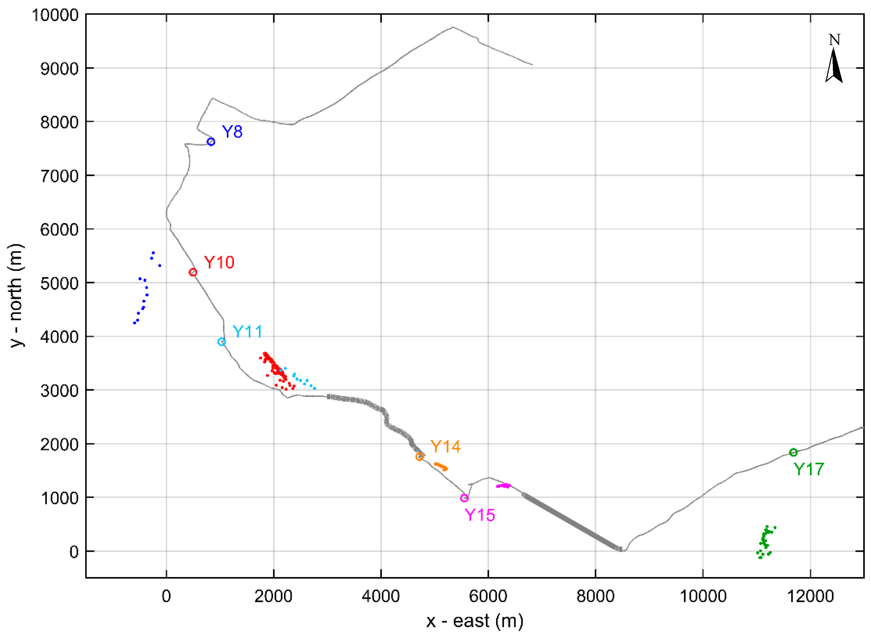
In
Figure 24, the horizontal localization results from the various stations are combined after selecting one of the two symmetrical solutions for each case, using the same criteria as in the case of sperm whale X. The consecutive thick grey dots along the vessel track denote the locations where the boat was next to whale Y (slightly to its side or right behind it) during surfacing. The vessel location in the middle of each station is marked by a circle of different color—the same color is used for the corresponding localization results (dots). The localization results from all stations are generally aligned with each other and also with the whale locations during surfacing (heavy lines). This verifies the range and azimuth estimation and describes a course of the whale from the northwest to the southeast.
5. Discussion and Conclusions
In this work, the Bayesian localization method introduced in [
20] was tested in two field experiments, one in shallow water and one in deep water. In the second experiment, in addition to the deployed source (pinger), the encounter with sperm whales—two different male whales on subsequent days—gave the opportunity for additional application and testing of the localization method, in which case the verifications came from actual encounters with the animals when they ascended to the surface.
The method uses the time difference of direct and surface-reflected arrivals of pulsed signals at two hydrophones of known/measured depths and also a measured sound speed profile to account for refraction assuming range independence. Range dependence of the medium is not expected to be significant over ranges 2–4 km (typical ocean mesoscale eddies have horizontal scales of the order of 100 km) except across very strong ocean fronts, which was not the case in the experiments presented here. On the other hand, the bathymetry can be strongly range dependent even over short ranges; in that case, direct and surface-reflected arrivals are not affected, care must still be taken to separate them from any bottom-reflected arrivals.
The Bayesian approach, combined with linearization of the problem and relying on ray theory, accounts for uncertainties in measured quantities (TDOAs, hydrophone depths, sound speed profile) and allows for quantification of the induced localization uncertainty. According to theory, the errors in range and depth estimation are smallest when the source and the hydrophone array are aligned in the horizontal (endfire), and largest when the source is perpendicular to the hydrophone array (broadside), and further they increase with source range. On the other hand, bearing errors have a reciprocal behavior with respect to the source azimuth; they are largest close to endfire and smallest close to broadside. Further, localization errors increase as the source approaches the sea surface or the vertical under the hydrophones.
In all cases, the error behavior in the localization experiments was found to be in agreement with the above theoretical conclusions, and tradeoffs between range/depth and bearing estimation accuracy were nicely demonstrated in cases where the array changed its orientation during stations, such as station A5 in the shallow-water experiments where range/depth errors dropped by ~75% in the course of one and the same station, or station Y10 in the localization of whale Y off Palaiochora where the error in bearing estimation also dropped by about the same percentage, from 20° to 5° RMS. Errors at long ranges were large. A significant improvement in such cases, particularly in cases of stationary targets, can be obtained by averaging, which leads to error reduction by a factor inversely proportional to the square root of the number of samples averaged. Averaging was applied in the cases of stations A1 in the shallow-water experiment at a range of ~1.5 km and B3 in the deep-water experiment at a range of ~3 km. A further source of errors is surface roughness which made its presence clear in the deep-water experiment in the form of error increase in the TDOAs between direct and surface-reflected arrivals, which in turn led to larger localization uncertainties.
In the case of sperm whales, localization in the horizontal was necessary for verification purposes. This type of localization relies on knowledge about the array geometry. In this connection, a simple model was used for the array geometry, which combines the measured hydrophone depths with information about the vessel track from GPS and hydrophone separation, taking into account the cable lengths. The implementation of this simple model in the analysis software used in the field enabled the successful localization of the two sperm whales. Interestingly, at the stations where there were significant changes in array orientation the model produced azimuthally concentrated solutions on the correct side of the array, as was verified by appropriate maneuvers (course changes) of the towing vessel as well as by the overall coherence of solutions from the various stations. The ultimate verification of the localization in the horizontal was the fact that the two whales were found and visually observed when they surfaced; with range/depth estimation only, it would have been nearly impossible to find the animals. The model for the array geometry could be further improved by using hydrodynamic modeling to describe the behavior of the towline and the hydrophone array.
All cases presented here involved localization of a single source. Localization of multiple sources could be possible if the corresponding signals are clearly distinguished (do not overlap) in the time domain. Still, in that case tracking and identification—association between location estimates and sources—would be necessary, a task that is not addressed in this work. With the existing hydrophone array, localizations were performed successfully up to ranges of about 3.5 km; the main limiting factors for localization at longer ranges were the loss of resolution direct and surface-reflected arrivals as well as the self-noise of the hydrophones.
The separation between direct and surface-reflected arrivals increases with hydrophone and source depth and decreases with source range. In localization, there is usually no control over the source location—only the hydrophone depths can be controlled. Thus, hydrophone depth is an important factor for the resolution of direct and surface-reflected arrivals; an increase in hydrophone depth increases the separation between direct and surface-reflected arrivals and thus allows for localization to longer ranges; further, an increase in hydrophone depth also contributes to error reduction. On the other hand, even hydrophone configurations that produce poor resolution between direct and surface-reflected arrivals can still be used for bearing estimation, using, e.g., the simple bearing estimation approach [
5], which relies only on direct arrivals, provided that there is information about the orientation of the hydrophone array.
Last but not least, localization requires sufficiently high signal-to-noise ratio, such that arrivals of the emitted signal can be detected and TDOAs reliably estimated. Both detection capability and travel-time accuracy deteriorate with decreasing SNR, as described by the passive sonar equation and the Cramér–Rao lower bound, respectively. In this respect, the relatively high self-noise levels of the hydrophone array used here turned out to be a limiting factor on maximum localization range. Part of the noise was due to the electronics and part due to the fastening of the two hydrophone arrays, with the longer cable sometimes tapping the front hydrophone. It is anticipated that the use of low-noise hydrophones attached to a single cable would enable high-quality recordings and localization to longer ranges.


