InSAR-Constrained Interseismic Deformation and Potential Seismogenic Asperities on the Altyn Tagh Fault at 91.5–95°E, Northern Tibetan Plateau


Abstract
: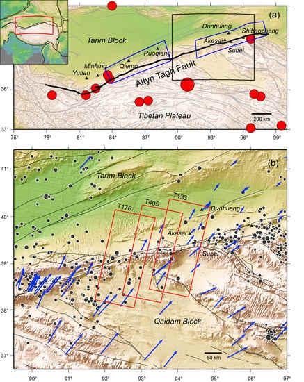
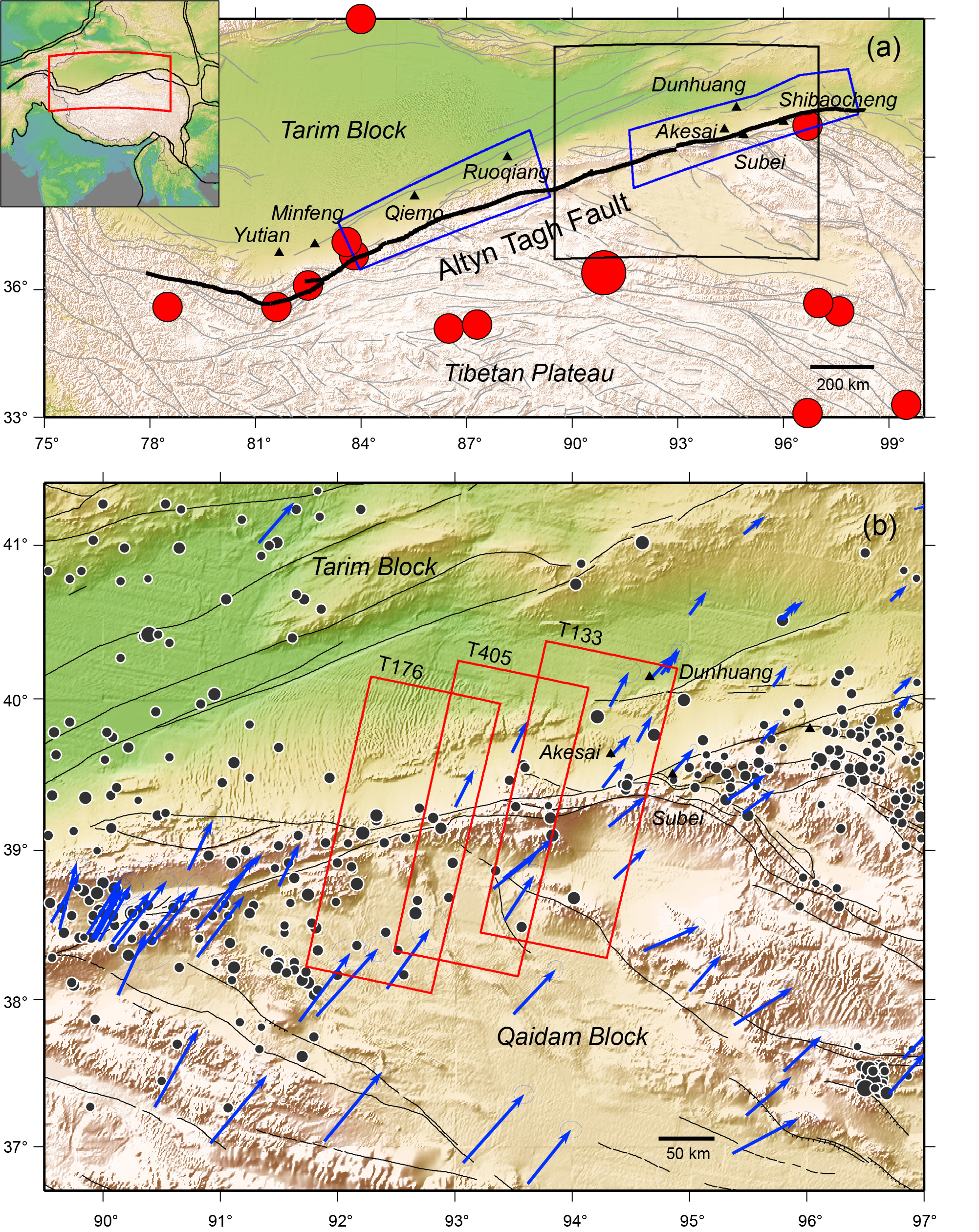
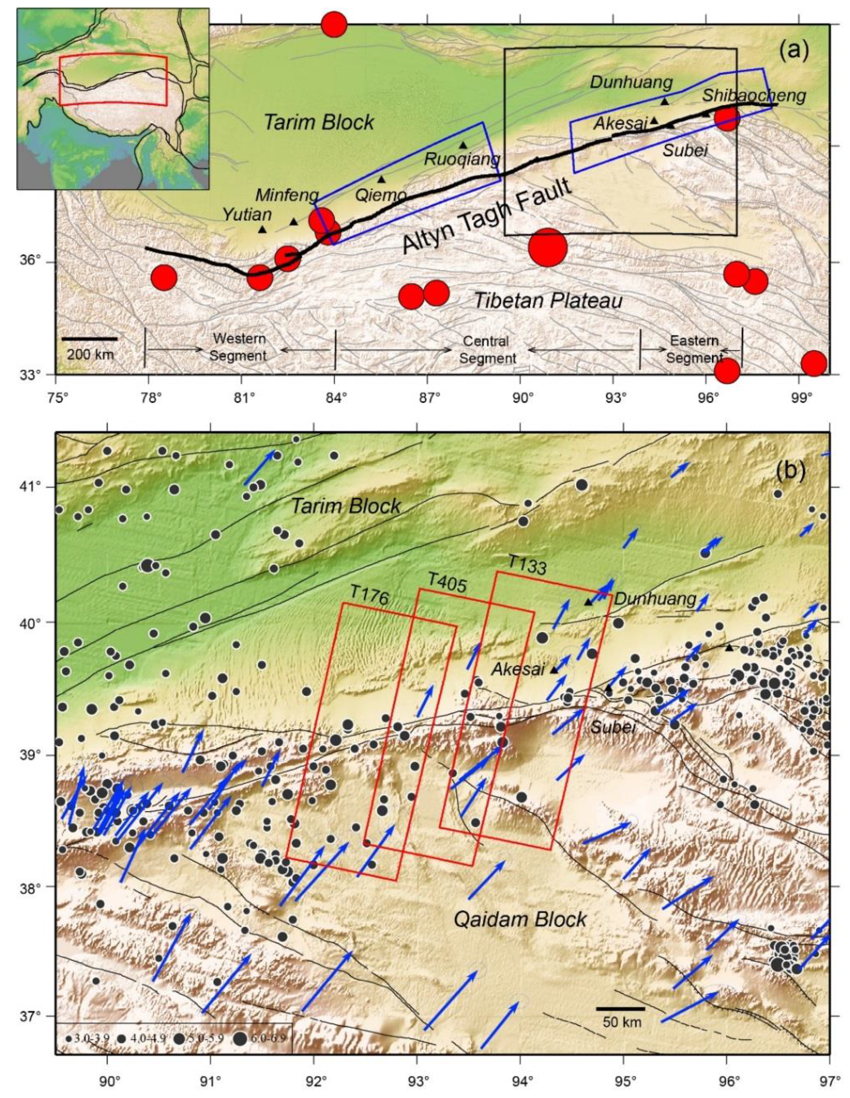
1. Introduction
2. InSAR Observations
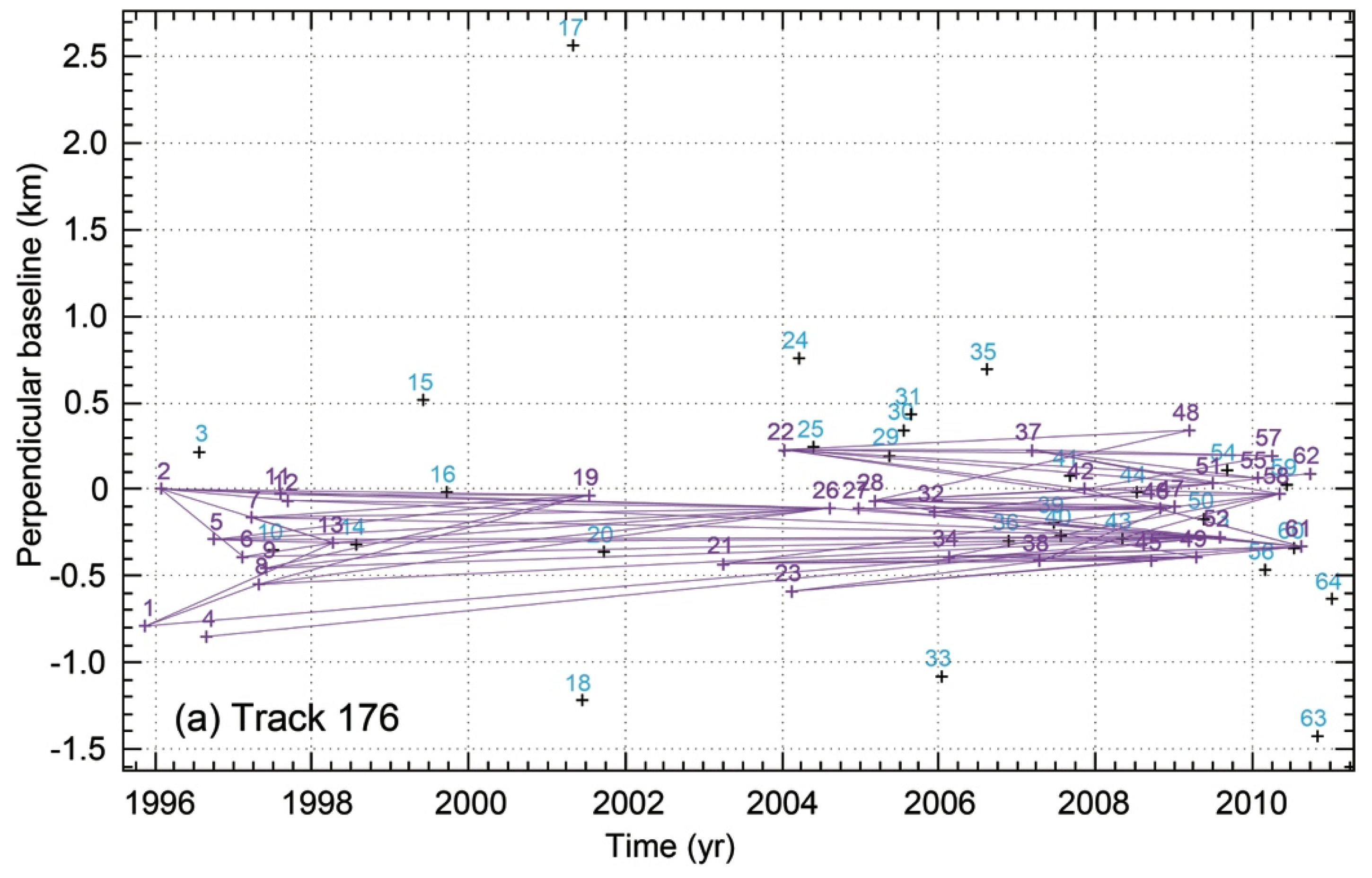
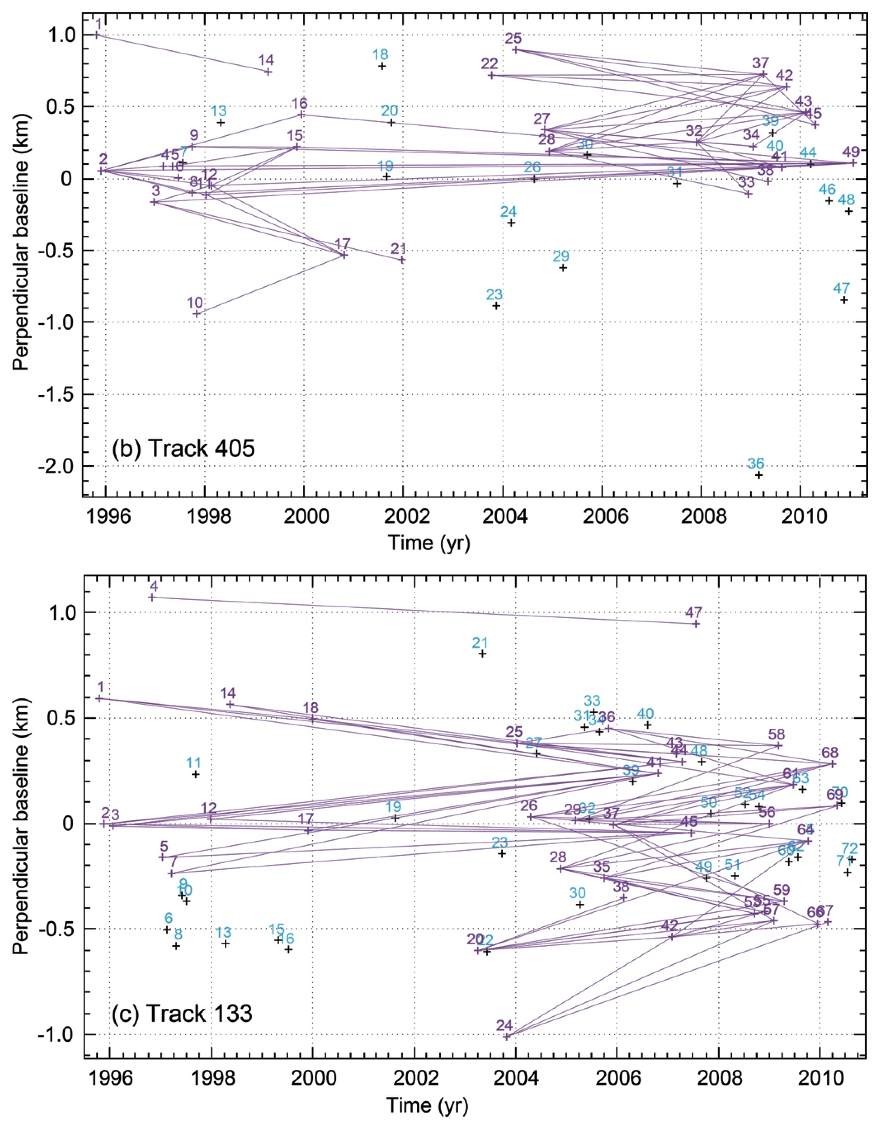
2.1. InSAR Data Processing Strategy
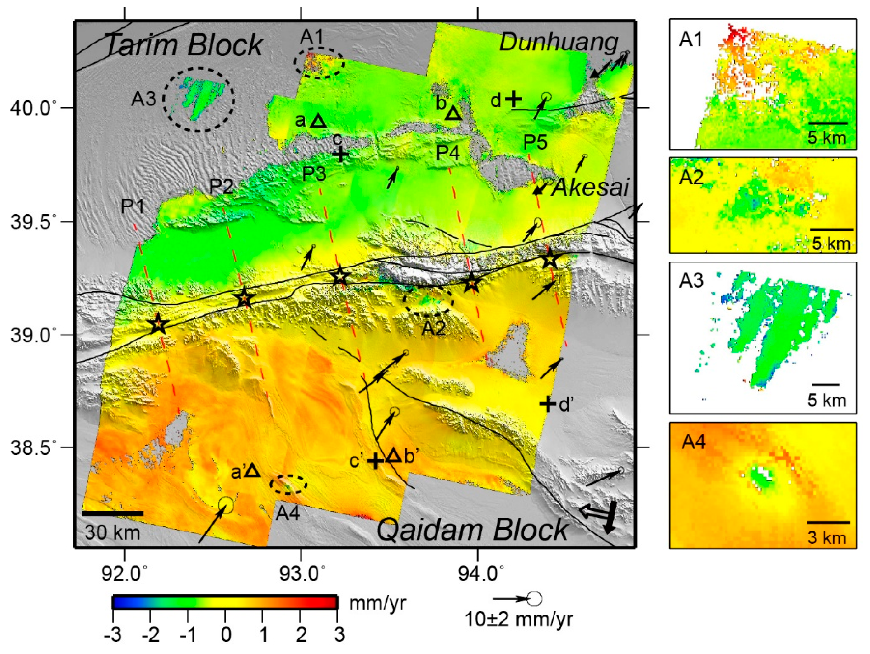
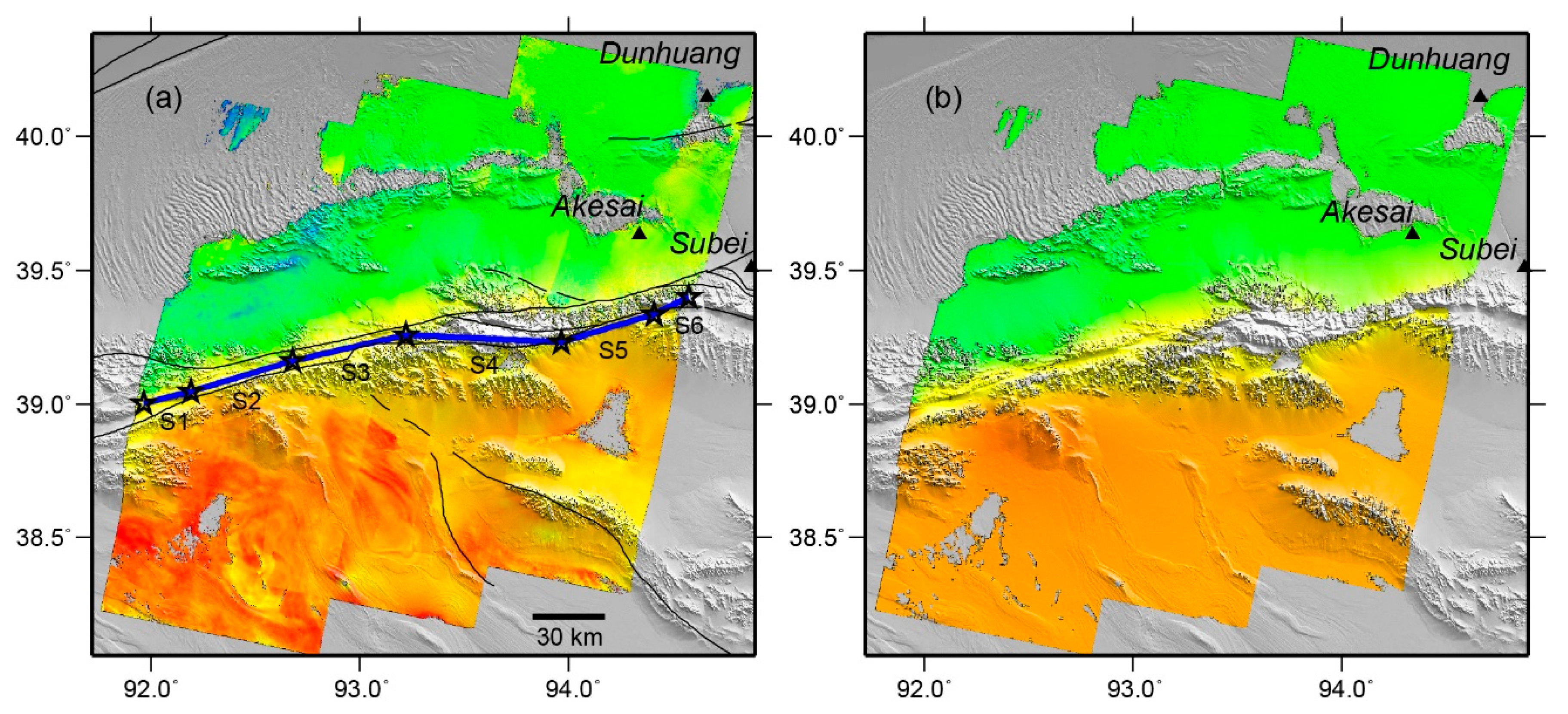
2.2. InSAR Velocity Field
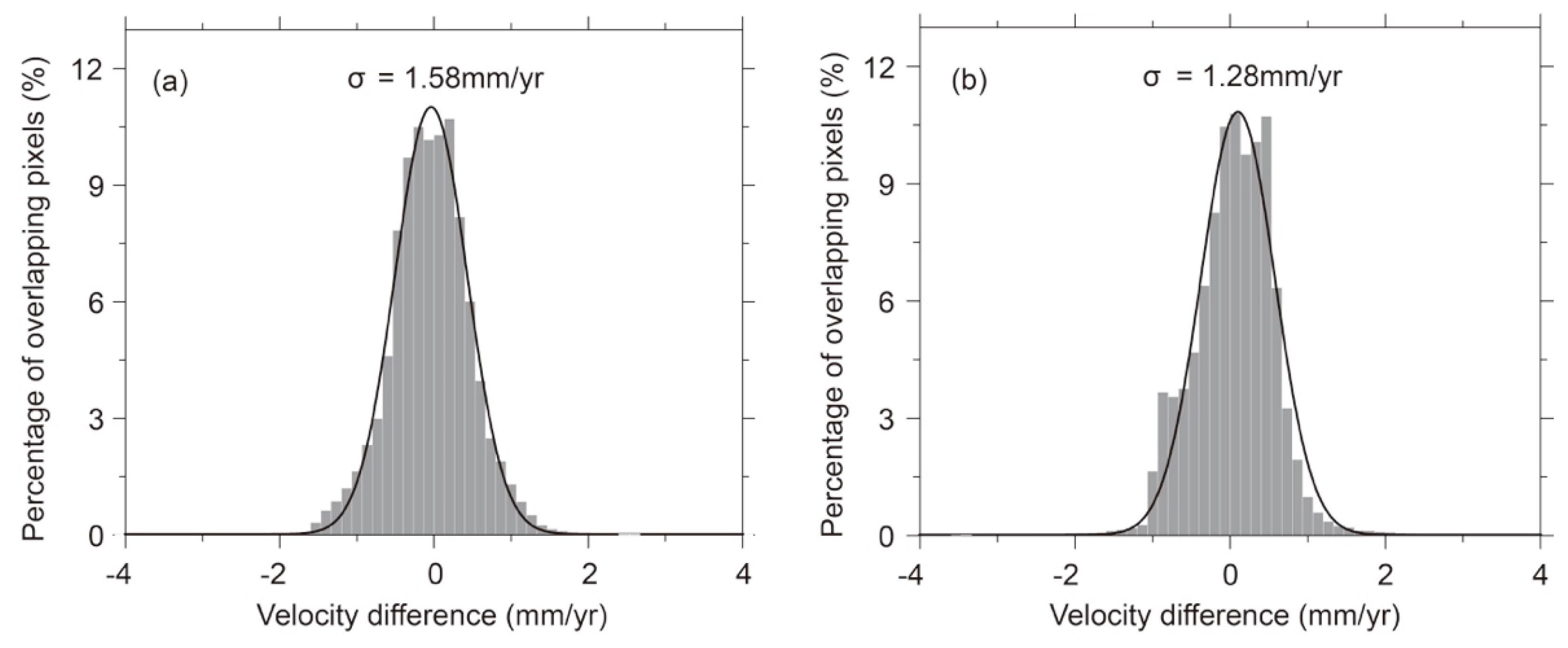
2.3. Evaluation of the InSAR-Derived Velocity
2.3.1. Validation of Overlapping Regions from Adjacent Tracks
2.3.2. Comparison with GPS Data
3. Interseismic Deformation Modeling
3.1. Fault Geometry
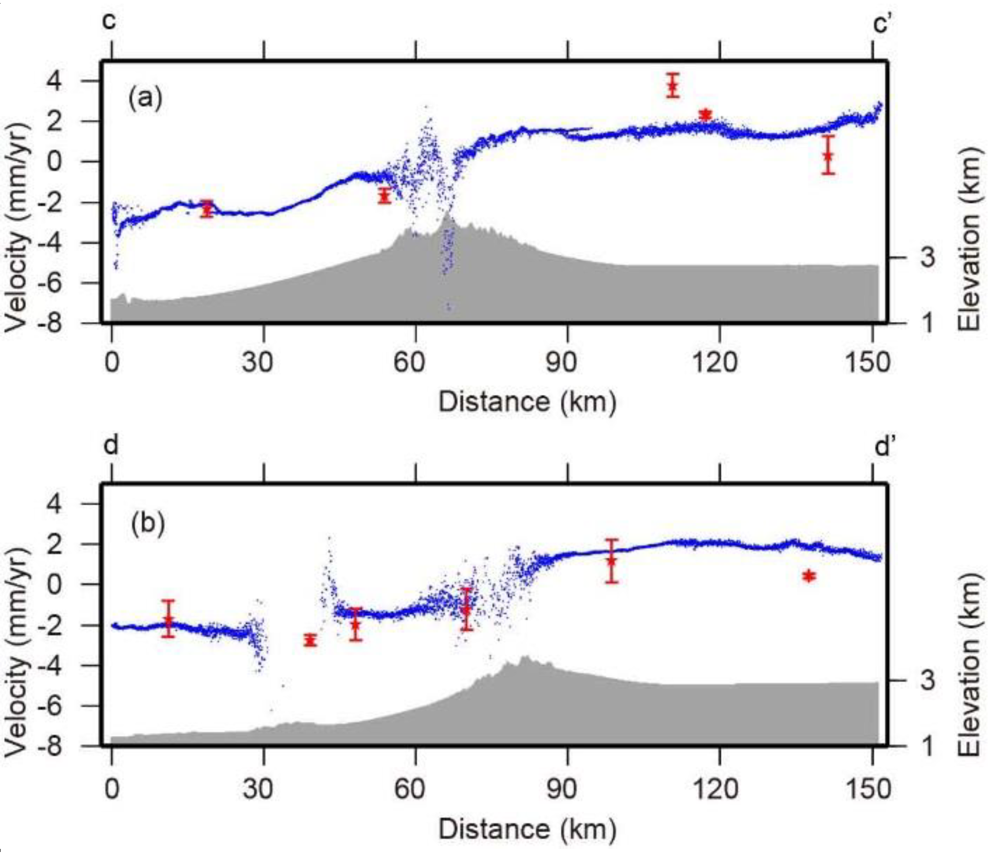
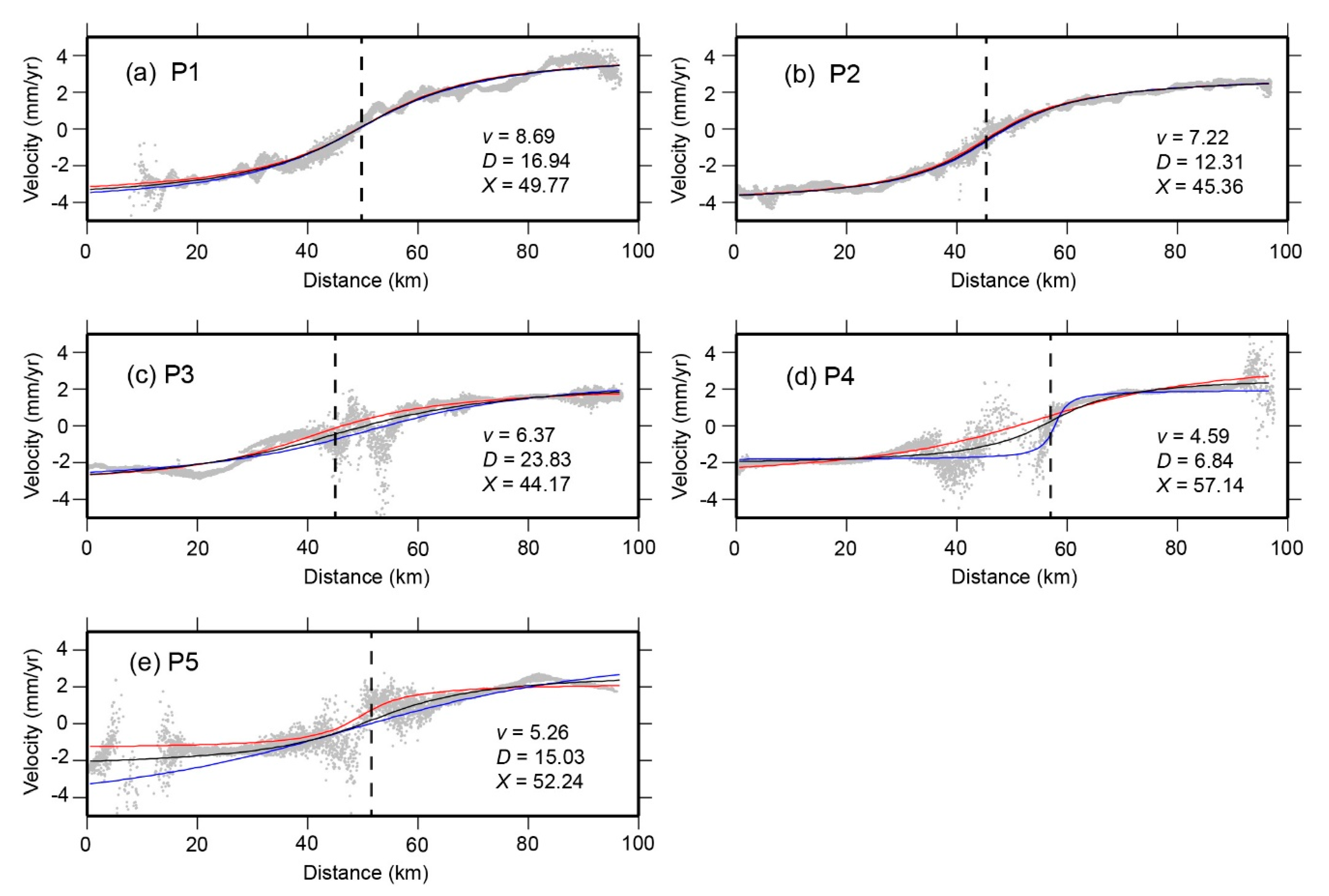
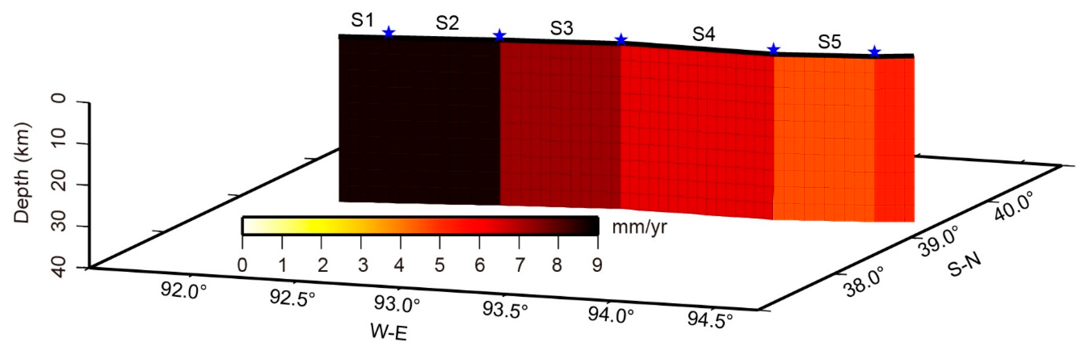
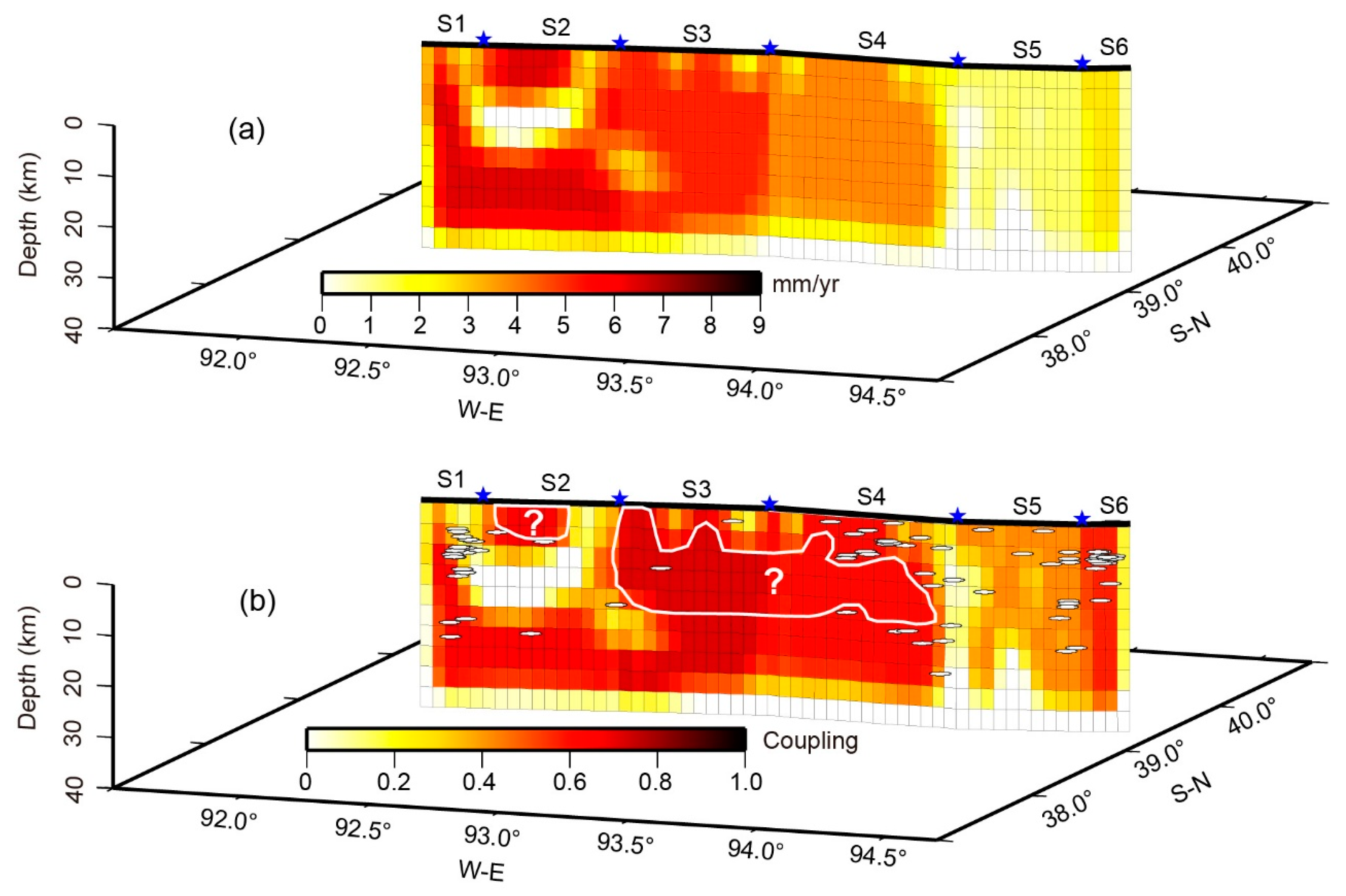
3.2. Slip Deficit Rates Distribution along the ATF at 91.5–95°E
3.2.1. Preprocessing InSAR Deformation Results
3.2.2. Modeling Approach
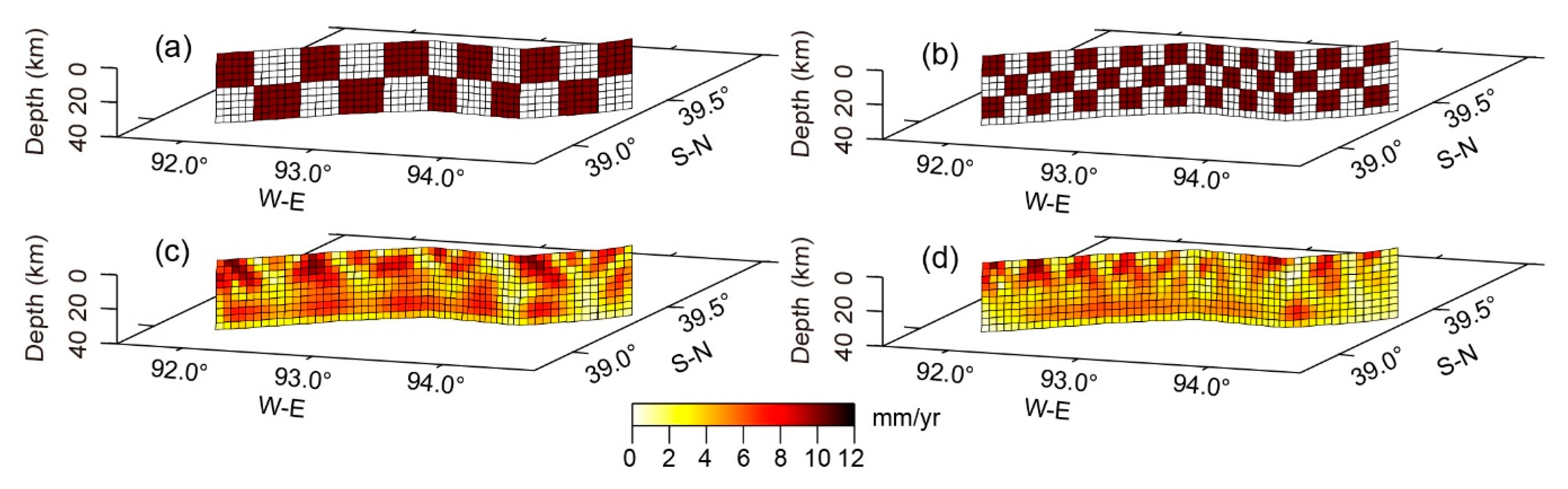
3.2.3. Modeling Results
4. Discussion
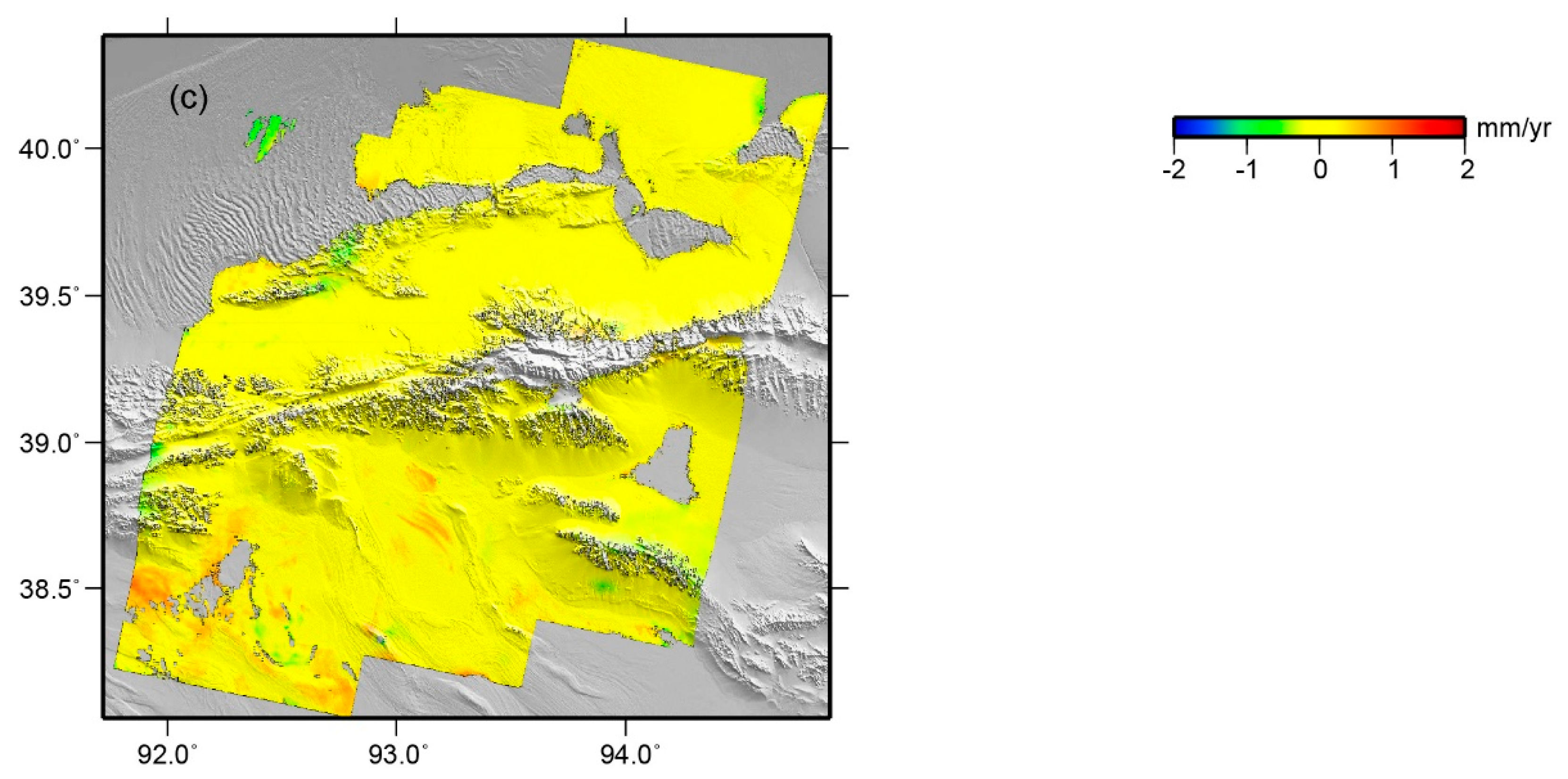
4.1. Local Nontectonic Deformation Detected in the InSAR Map
4.2. Possible Tectonic Deformation Mechanism of the Northern Tibetan Plateau
4.3. Comparison of Coupling and Seismicity
4.4. Seismic Potential of the ATF at 91.5–95°E
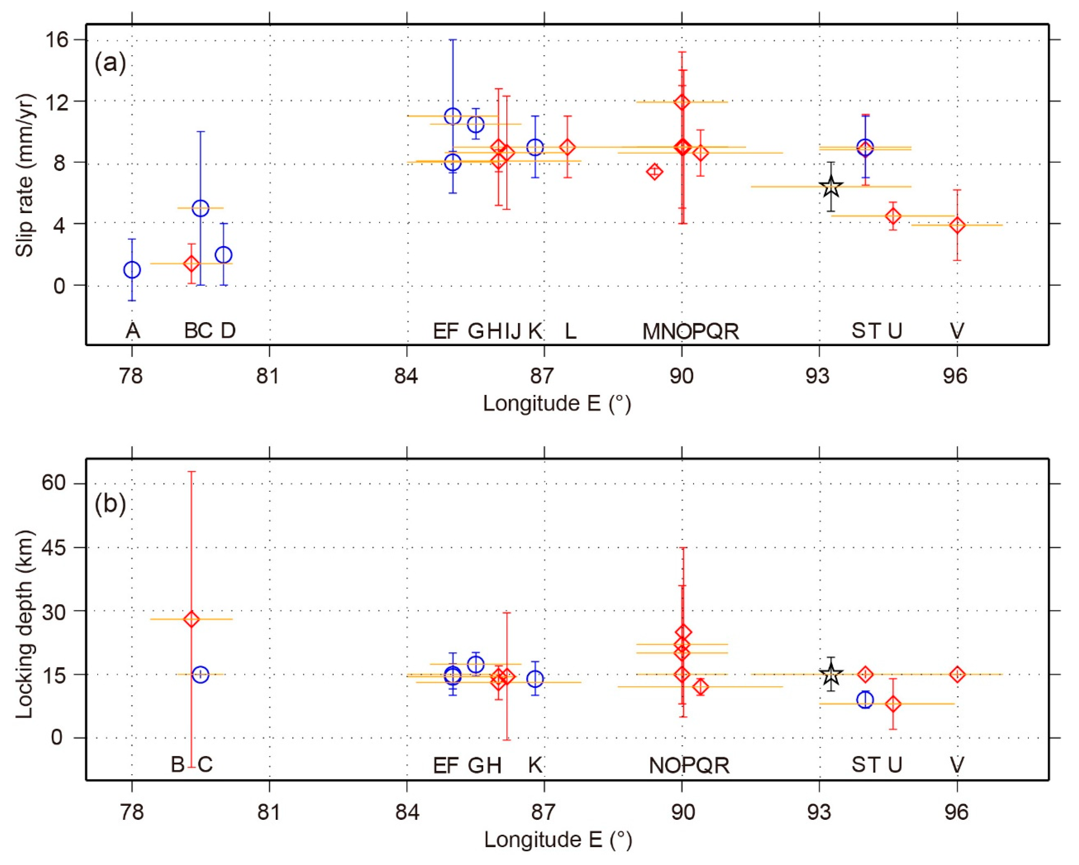
4.5. Present-Day Slip Rate and Locking Depth Variations along the Entire ATF from GPS and InSAR
5. Conclusions
Author Contributions
Funding
Acknowledgments
Conflicts of Interest
References
- Avouac, J.P.; Tapponnier, P. Kinematic model of active deformation in central Asia. Geophys. Res. Lett. 1993, 20, 895–898. [Google Scholar] [CrossRef] [Green Version]
- England, P.; Molnar, P. Active deformation of Asia: From kinematics to dynamics. Science 1997, 278, 647–650. [Google Scholar] [CrossRef]
- Li, H. The Formation Age of Altyn Tagh Fault Zone and the Contribution of Its Strike-Slipping to the Uplifting of North Qinghai-Tibet Plateau. Ph.D. Thesis, Chinese Academy Geological Sciences, Beijing, China, 2001. (In Chinese). [Google Scholar]
- Li, H.; Xu, Z.; Chen, W. The southern margin strike-slip fault zone of the East Kunlun Mountains: An important consequence from intracontinental deformation. Cont. Dyn. 1996, 1, 146–155. [Google Scholar]
- Li, H.; Yang, J.; Xu, Z.; Wu, C.; Wan, Y.; Shi, R.; Liou, J.G.; Tapponnier, P.; Ireland, T.R. Geological and chronological evidence of Indo-Chinese strike-slip movement in the Altyn Tagh fault zone. Chin. Sci. Bull. 2002, 47, 27–32. [Google Scholar] [CrossRef]
- Li, H.; Yang, J. Evidence for Cretaceous uplift of the northern Qinghai-Tibetan plateau. Earth Sci. Front. 2004, 11, 345–359. (In Chinese) [Google Scholar]
- Xie, F.; Liu, G. Analysis of Neotectonic stress field in area of the central segment of Altyn Tagh fault zone, China. Earthq. Res. China 1989, 5, 26–36. [Google Scholar]
- Tapponnier, P.; Zhiqin, X.; Roger, F.; Meyer, B.; Arnaud, N.; Wittlinger, G.; Jingsui, Y. Oblique stepwise rise and growth of the Tibet Plateau. Science 2001, 294, 1671–1677. [Google Scholar] [CrossRef] [PubMed]
- Xu, X.; Wu, X.; Yu, G.; Li, K. Seismo-geological signatures for identifying M ≥ 7.0 earthquake risk areas and their preliminary application in mainland China. Seismol. Geol. 2017, 39, 219–275. (In Chinese) [Google Scholar] [CrossRef]
- Zheng, G.; Wang, H.; Wright, T.J.; Lou, Y.; Zhang, R.; Zhang, W.; Shi, C.; Huang, J.; Wei, N. Crustal deformation in the India-Eurasia collision zone from 25 years of GPS measurements. J. Geophys. Res. Solid Earth 2017, 122, 9290–9312. [Google Scholar] [CrossRef]
- Bai, M. Kinematic and dynamic characteristics of the Altyn Tagh active fault zone. Xinjiang Geol. 1992, 10, 57–61. (In Chinese) [Google Scholar]
- Xu, X.; Klinger, Y.; Tapponnier, P.; Chen, G.; Li, K.; Tan, X.B. Long-Term Faulting Behavior of Eastern Altyn Tagh Fault, North. Tibetan Plateau; 2015 AGU Fall Meeting; AGU: Washington, DC, USA, 2015. [Google Scholar]
- Department of Earthquake Damage and Defense of China Earthquake Administration. Catalogue of Chinese Earthquakes (1912–1990) Ms ≥ 4.7; China Science and Technology Press: Beijing, China, 1999. (In Chinese)
- Li, Y.; Chen, L.; Liu, S.; Yang, S.; Yang, X.; Zhang, G. Coseismic coulomb stress changes caused by the Mw6.9 Yutian earthquake in 2014 and its correlation to the 2008 Mw7.2 Yutian earthquake. J. Asian Earth Sci. 2015, 105, 468–475. [Google Scholar] [CrossRef]
- Wright, T.J.; Parsons, B.; England, P.C.; Fielding, E.J. InSAR observations of low slip rates on the major faults of western Tibet. Science 2004, 305, 236–239. [Google Scholar] [CrossRef] [PubMed]
- Wang, H.; Wright, T.J. Satellite geodetic imaging reveals internal deformation of western Tibet. Geophys. Res. Lett. 2012, 39, L07303. [Google Scholar] [CrossRef]
- Daout, S.; Doin, M.-P.; Peltzer, G.; Lasserre, C.; Socquet, A.; Volat, M.; Sudhaus, H. Strain partitioning and present-day fault kinematics in NW Tibet from Envisat SAR interferometry. J. Geophys. Res. Solid Earth 2018, 123, 2462–2483. [Google Scholar] [CrossRef]
- Elliott, J.R.; Biggs, J.; Parsons, B.; Wright, T.J. InSAR slip rate determination on the Altyn Tagh Fault, northern Tibet, in the presence of topographically correlated atmospheric delays. Geophys. Res. Lett. 2008, 35, 82–90. [Google Scholar] [CrossRef]
- Zhu, S.; Xu, C.; Wen, Y.; Liu, Y. Interseismic deformation of the Altyn Tagh fault determined by Interferometric Synthetic Aperture Radar (InSAR) measurements. Remote Sens. 2016, 8, 233. [Google Scholar] [CrossRef]
- Bendick, R.; Bilham, R.; Freymueller, J.; Larson, K.; Yin, G. Geodetic evidence for a low slip rate in the altyn tagh fault system. Nature 2000, 404, 69–72. [Google Scholar] [CrossRef] [PubMed]
- Jolivet, R.; Cattin, R.; Chamot-Rooke, N.; Lasserre, C.; Peltzer, G. Thin-plate modeling of interseismic deformation and asymmetry across the Altyn Tagh fault zone. Geophys. Res. Lett. 2008, 35, L02309. [Google Scholar] [CrossRef]
- He, J.; Philippe, V.; Jean, C.; Wang, W.; Lu, S.; Ku, W.; Xia, W.; Bilham, R. Nailing down the slip rate of the altyn tagh fault. Geophys. Res. Lett. 2013, 40, 5382–5386. [Google Scholar] [CrossRef]
- Shen, Z.K.; Wang, M.; Li, Y.; Jackson, D.D.; Yin, A.; Dong, D.; Pang, F. Crustal deformation along the Altyn Tagh fault system, western China, from GPS. J. Geophys. Res. Solid Earth 2001, 106, 30607–30621. [Google Scholar] [CrossRef] [Green Version]
- Shen, L.; Hooper, A.; Elliott, J.; Wright, T. Interseismic deformation along the Altyn Tagh fault, Tibet: Implications for shallow creep. Geophys. Res. Abstr. 2018, 20, EGU2018-1191-2. [Google Scholar]
- Vernant, P. What can we learn from 20 years of interseismic GPS measurements across strike-slip faults? Tectonophysics 2015, 644–645, 22–39. [Google Scholar] [CrossRef]
- Wallace, K.; Yin, G.; Bilham, R. Inescapable slow slip on the Altyn Tagh fault. Geophys. Res. Lett. 2004, 31, L09613. [Google Scholar] [CrossRef]
- Wang, W.; Qiao, X.; Yang, S.; Wang, D. Present-day velocity field and block kinematics of Tibetan plateau from GPS measurements. Geophys. J. Int. 2017, 208, 1088–1102. [Google Scholar] [CrossRef]
- Zhang, P.Z.; Molnar, P.; Xu, X. Late Quaternary and present-day rates of slip along the Altyn Tagh Fault, northern margin of the Tibetan plateau. Tectonics 2007, 26, TC5010. [Google Scholar] [CrossRef]
- Zebker, H.A.; Rosen, P.A.; Hensley, S. Atmospheric effects in interferometric synthetic aperture radar surface deformation and topographic maps. J. Geophys. Res. Solid Earth 1997, 102, 7547–7563. [Google Scholar] [CrossRef] [Green Version]
- Kaneko, Y.; Avouac, J.-P.; Lapusta, N. Towards inferring earthquake patterns from geodetic observations of interseismic coupling. Nat. Geosci. 2010, 3, 363–369. [Google Scholar] [CrossRef] [Green Version]
- Manoochehr, S.; Bürgmann, R.; Taira, T. Implications of recent asperity failures and aseismic creep for time-dependent earthquake hazard on the Hayward fault. Earth Planet. Sci. Lett. 2013, 371–372, 59–66. [Google Scholar] [CrossRef]
- Ji, L.; Lu, Z.; Dzurisin, D.; Senyukov, S. Pre-eruption deformation caused by dike intrusion beneath Kizimen volcano, Kamchatka, Russia, observed by InSAR. J. Volcanol. Geotherm. Res. 2013, 256, 87–95. [Google Scholar] [CrossRef]
- Ji, L.; Hu, Y.; Wang, Q.; Xu, X.; Xu, J. Large-scale deformation caused by dyke intrusion beneath eastern Hainan Island, China observed using InSAR. J. Geodyn. 2015, 88, 52–58. [Google Scholar] [CrossRef]
- Ji, L.; Zhang, Y.; Wang, Q.; Xin, Y.; Li, J. Detecting land uplift associated with enhanced oil recovery using InSAR in the Karamay oil field, Xinjiang, China. Int. J. Remote Sens. 2016, 37, 1527–1540. [Google Scholar] [CrossRef]
- Werner, C.; Wegmüller, U.; Strozzi, T.; Wiesmann, A. GAMMA SAR and interferometric processing software. In Proceedings of the ERS-Envisat Symposium, Gothenburg, Sweden, 16–20 October 2000. [Google Scholar]
- Massonnet, D.; Feigl, K. Radar interferometry and its application to changes in the Earth’s surface. Rev. Geophys. 1998, 36, 441–500. [Google Scholar] [CrossRef]
- Rosen, P.A.; Hensley, S.; Joughin, I.R.; Li, F.K.; Madsen, S.N.; Rodriguez, E.; Goldstein, R.M. Synthetic aperture radar interferometry. Proc. IEEE 2000, 88, 333–380. [Google Scholar] [CrossRef]
- Farr, T.G.; Kobrick, M. Shuttle Radar Topography Mission produces a wealth of data. Eos Trans. AGU 2000, 81, 583–585. [Google Scholar] [CrossRef]
- Goldstein, R.M.; Werner, C.L. Radar Interferogram Filtering for Geophysical Applications. Geophys. Res. Lett. 1998, 25, 4035–4038. [Google Scholar] [CrossRef]
- Costantini, M. A novel phase unwrapping method based on network programming. IEEE Trans. Geosci. Remote Sens. 1998, 36, 813–821. [Google Scholar] [CrossRef]
- Savage, J.C.; Burford, R.O. Geodetic determination of relative plate motion in Central California. J. Geophys. Res. 1973, 78, 832–845. [Google Scholar] [CrossRef]
- Gray, A.L.; Mattar, K.E.; Sofko, G. Influence of ionospheric electron density fluctuations on satellite radar interferometry. Geophys. Res. Lett. 2000, 27, 1451–1454. [Google Scholar] [CrossRef] [Green Version]
- Jolivet, R.; Grandin, R.; Lasserre, C.; Doin, M.P.; Peltzer, G. Systematic InSAR tropospheric phase delay corrections from global meteorological reanalysis data. Geophys. Res. Lett. 2011, 38, 351–365. [Google Scholar] [CrossRef]
- Zebker, H.A.; Goldstein, R.M. Topographic mapping from interferometric synthetic aperture radar observations. J. Geophys. Res. Solid Earth 1986, 91, 4993–4999. [Google Scholar] [CrossRef]
- Wright, T.; Parsons, B.; Fielding, E. Measurement of interseismic strain accumulation across the North Anatolian Fault by satellite radar interferometry. Geophys. Res. Lett. 2001, 28, 2117–2120. [Google Scholar] [CrossRef] [Green Version]
- Biggs, J.; Wright, T.; Lu, Z.; Parsons, B. Multi-interferogram method for measuring interseismic deformation: Denali Fault, Alaska. Geophys. J. Int. 2007, 170, 1165–1179. [Google Scholar] [CrossRef] [Green Version]
- Wang, H.; Wright, T.J.; Biggs, J. Interseismic slip rate of the northwestern Xianshuihe fault from InSAR data. Geophys. Res. Lett. 2009, 36. [Google Scholar] [CrossRef] [Green Version]
- Lyons, S.; Sandwell, D. Fault creep along the southern San Andreas from interferometric synthetic aperture radar, permanent scatterers, and stacking. J. Geophys. Res. Solid Earth 2003, 108, 2047. [Google Scholar] [CrossRef]
- Xiao, Q.; Shao, G.; Liu-Zeng, J.; Oskin, M.E.; Zhang, J.; Zhao, G.; Wang, J. Eastern termination of the Altyn Tagh Fault, western China: Constraints from a magnetotelluric survey. J. Geophys. Res. Solid Earth 2015, 120, 2838–2858. [Google Scholar] [CrossRef] [Green Version]
- Ma, Y.; Ma, H. Discussion on earthquake risk and characteristics of seismic activity in the middle-east section along the Altun Tagh fault zone. Plateau Earthq. Res. 2014, 26, 1–6. [Google Scholar]
- Wang, R.; Diao, F.; Hoechner, A. SDM—A geodetic inversion code incorporating with layered crust structure and curved fault geometry. Geophys. Res. Abstr. 2013, 15, EGU2013-2411-1. [Google Scholar]
- Ji, L.; Wang, Q.; Xu, J.; Feng, J. The 1996 Mw 6.6 Lijiang earthquake: Application of JERS-1 SAR interferometry on a typical normal-faulting event in the northwestern Yunnan rift zone, SW China. J. Asian Earth Sci. 2017, 146, 221–232. [Google Scholar] [CrossRef]
- Diao, F.; Xiong, X.; Wang, R. Mechanisms of transient postseismic deformation following the 2001 Mw 7.8 Kunlun (China) earthquake. Pure Appl. Geophys. 2011, 168, 767–779. [Google Scholar] [CrossRef]
- Reinoza, C.; Jouanne, F.; Audemard, F.A.; Schmitz, M.; Beck, C. Geodetic exploration of strain along the EI Pilar fault in northeastern Venezuela. J. Geophys. Res. Solid Earth 2015, 120, 1993–2013. [Google Scholar] [CrossRef]
- Beltran, L.P.; Pathier, E.; Jouanne, F.; Vassallo, R.; Reinoza, C.; Audemard, F.; Volat, M. Spatial and temporal variations in creep rate along the El Pilar fault at the Caribbean-South American plate boundary (Venezuela), from InSAR. J. Geophys. Res. Solid Earth 2016, 121, 8276–8296. [Google Scholar] [CrossRef]
- Jouanne, F.; Mugnier, J.L.; Sapkota, S.N.; Bascou, P.; Pecher, A. Estimation of coupling along the main himalayan thrust in the central Himalaya. J. Asian Earth Sci. 2017, 133, 62–71. [Google Scholar] [CrossRef]
- Laske, G.; Masters, G.; Ma, Z.; Pasyanos, M. Update on CRUST1.0—A 1-degree global model of earth’s crust. In Proceedings of the EGU General Assembly 2013, Vienna, Austria, 7–12 April 2013. [Google Scholar]
- Lay, T.; Kanamori, H. Earthquake doublets in the Solomon islands. Phys. Earth Planet. Inter. 1980, 21, 283–304. [Google Scholar] [CrossRef]
- Ryder, I.; Bürgmann, R. Spatial variations in slip deficit on the central San Andreas fault from InSAR. Geophys. J. Int. 2008, 175, 837–852. [Google Scholar] [CrossRef]
- Jolivet, R.; Simons, M.; Agram, P.S.; Duputel, Z.; Shen, Z. Aseismic slip and seismogenic coupling along the central San Andreas Fault. Geophys. Res. Lett. 2015, 42, 297–306. [Google Scholar] [CrossRef] [Green Version]
- Aktuğ, B.; Doğru, A.; Özener, H.; Peyret, M. Slip rates and locking depth variation along central and easternmost segments of North Anatolian fault. Geophys. J. Int. 2015, 202, 2133–2149. [Google Scholar] [CrossRef]
- Tolomei, C.; Salvi, S.; Boncori, J.M.; Pezzo, G. InSAR measurement of crustal deformation transients during the earthquake preparation processes: A review. Boll. Geofis. Teor. Appl. 2015, 56, 151–166. [Google Scholar] [CrossRef]
- Elliott, J.R.; Walters, R.J.; Wright, T.J. The role of space-based observation in understanding and responding to active tectonics and earthquakes. Nat. Commun. 2016, 7, 13844. [Google Scholar] [CrossRef] [PubMed] [Green Version]


| Track | Satellites | Number of Images and Interferograms | Images Used | Interferograms Used |
|---|---|---|---|---|
| 176 | ERS-1/2 | 24 (119) | 13 | 49 |
| Envisat | 40 (435) | 20 | 65 | |
| 405 | ERS-1/2 | 25 (113) | 16 | 35 |
| Envisat | 24 (123) | 13 | 43 | |
| 133 | ERS-1/2 | 27 (162) | 13 | 35 |
| Envisat | 45 (519) | 23 | 60 |
| NO. | Bperp (Meter) | Btemp (Day) |
|---|---|---|
| 1 | 400 m < Bperp < 600 m | 350 day < Delta_T ≤ 500 day |
| 2 | 200 m < Bperp ≤ 400 m | 500 day < Delta_T ≤ 1000 day |
| 3 | Bperp ≤ 200 m | 1000 day < Delta_T |
| NO. | Longitude (°E) | Slip Rate (mm/year) | Locking Depth (km) | Data Source | Reference |
|---|---|---|---|---|---|
| A | 78 | 1 ± 2 | NA | InSAR | [16] |
| B | 79–80 | 5 ± 5 | 15 | InSAR | [15] |
| C | 78.4–80.2 | 1.4 ± 1.3 | 28 ± 35 | GPS | [10] |
| D | 80 | 2 ± 2 | NA | InSAR | [16] |
| E | 84–86 | 11 ± 5 | 15 (+10/+20) | InSAR | [18] |
| F | 84–86 | 8 ± 0.7 | 14.5 ± 3 | InSAR | [19] |
| G | 84.5–86.5 | 10.5 ± 1.0 | 17.4 (−3/+2.6) | InSAR | [17] |
| H | 84.2–87.8 | 8.1 ± 0.7 | 13 ± 4 | GPS | [10] |
| I | 84.8–87.5 | 8.6 (−3.2/+4.2) | 14.5 (−14.5/+15.5) | GPS | [25] |
| J | 85–90 | 9 ± 2 | NA | GPS | [23] |
| K | 85.6–86.4 | 9.0 (−3.2/+4.4) | 14.5 | GPS | [22] |
| L | 86.8 | 9 ± 2 | 14 ± 4 | InSAR | [24] |
| M | 89.4 | 7.4 ± 0.2 | NA | GPS | [27] |
| N | 89–91 | 9 ± 5 | 8–36 | GPS | [20] |
| O | 89–91 | 9 ± 4 | 20 | GPS | [26] |
| P | 89–91 | 11.9 ± 3.3 | 15 | GPS | [28] |
| Q | 88.7–91.4 | 9 ± 5 | 25 (+5/−20) | GPS | [25] |
| R | 88.6–92.2 | 8.6 ± 1.5 | 12 ± 2 | GPS | [10] |
| S | 93–95 | 8–10 | 7–9 | InSAR | [21] |
| T | 93–95 | 8.8 ± 2.3 | 15 | GPS | [28] |
| U | 93.3–96 | 4.5 ± 0.9 | 8 ± 6 | GPS | [10] |
| V | 95–97 | 3.9 ± 2.3 | 15 | GPS | [28] |
| This Study | 91.5–95 | 6.4 ± 1.6 | 15 ± 4 | InSAR |
© 2018 by the authors. Licensee MDPI, Basel, Switzerland. This article is an open access article distributed under the terms and conditions of the Creative Commons Attribution (CC BY) license (http://creativecommons.org/licenses/by/4.0/).
Share and Cite
Liu, C.; Ji, L.; Zhu, L.; Zhao, C. InSAR-Constrained Interseismic Deformation and Potential Seismogenic Asperities on the Altyn Tagh Fault at 91.5–95°E, Northern Tibetan Plateau. Remote Sens. 2018, 10, 943. https://doi.org/10.3390/rs10060943
Liu C, Ji L, Zhu L, Zhao C. InSAR-Constrained Interseismic Deformation and Potential Seismogenic Asperities on the Altyn Tagh Fault at 91.5–95°E, Northern Tibetan Plateau. Remote Sensing. 2018; 10(6):943. https://doi.org/10.3390/rs10060943
Chicago/Turabian StyleLiu, Chuanjin, Lingyun Ji, Liangyu Zhu, and Chaoying Zhao. 2018. "InSAR-Constrained Interseismic Deformation and Potential Seismogenic Asperities on the Altyn Tagh Fault at 91.5–95°E, Northern Tibetan Plateau" Remote Sensing 10, no. 6: 943. https://doi.org/10.3390/rs10060943