Identification of Stable Backscattering Features, Suitable for Maintaining Absolute Synthetic Aperture Radar (SAR) Radiometric Calibration of Sentinel-1

Abstract

Measuring the absolute calibration constant is crucial for the radiometric calibration of synthetic aperture radar (SAR) systems. However, it is expensive to monitor the calibration constant continuously using manmade calibrators, and it is regionally restricted using the rainforest as the calibration field. In this study, the stability of SAR backscattering for common objects on the earth surface was analyzed, expecting to find the stable backscattering feature that could be used for maintaining absolute radiometric calibration. A database was established using Sentinel-1 dataset, and a classification model based on neural networks was proposed to extract the image slices of proper objects. Based on these, a temporal stable backscattering feature with a standard deviation of 0.19 dB was obtained from urban areas, and it was proved to be even more stable than the rainforest. Finally, the calibration scheme was given using this stable feature as a reference, which provided a new means of monitoring the SAR radiometric calibration constant.

1. Introduction

The measurement of the absolute calibration constant is vital to the radiometric calibration of synthetic aperture radar (SAR) systems, which influences the quantitative application of SAR, such as soil moisture mapping, marine parameters measurement, and biomass retrieval [1,2,3,4]. Manmade calibrators, like transponders, corner reflectors, and ground receivers, are commonly used to measure the calibration constant. They have known radar cross sections (RCSs) with a high radiometric accuracy (better than 0.2 dB) [5,6,7]. The calibrators are usually placed in a uniform and low noise field. The calibration constant is calculated as the difference between the calibrator’s true RCS and its image intensity. However, the layout and maintenance of calibrators is costly; therefore, the calibrator-based method can only be conducted a few times in the whole lifetime of the SAR [5], which influences the measurement accuracy of the constant. Monitoring of the constant is usually undertaken by the measurement of Amazon rainforest, which is a temporal stable and azimuthally isotropic natural target [8,9,10]. The measurements of Radarsat-1 show that, if it chose a suitable area in Amazon, the backscatter coefficients of rainforest in C-band SAR are concentrated on −6.5 dB with a standard deviation of less than 0.3 dB [11]. Therefore, its backscatter coefficient can be used as a calibration reference. However, the Amazon rainforest is located in a specific geographical area, so it can only be illuminated in the intervals of the observation tasks. Thus, the frequency of the constant measurement cannot be guaranteed.

Besides the manmade calibrators and rainforests, the researches about calibration reference mainly focus on deserts, oceans, and permanent scatters (PSs). The study about the Simpson Desert shows that its backscattering coefficients are consistently 12 dB with a root mean square error (RMSE) of 0.2 dB as time changes and the accuracy when it is used to cross-calibrate radar altimeters is about 1 dB [12]. However, the desert’s backscattering stability depends on the surface topography and soil moisture. Oceans can also be used to derive the calibration constant, using the empirical models of the relationship between the oceans’ backscatter coefficient and the wind speed. The accuracy is about 0.5 dB when it is used to calibrate ERS-2 SAR images [13]. Nevertheless, this method needs massive images to fit the model and then to obtain model parameters; so its accuracy is susceptible to the quantity and selection of dataset. Moreover, these two methods cannot resolve the regional-restricted problem and the accuracy is relatively low. The method based on PS has also been studied. PSs usually appear in urban areas, rocky areas, and some P-land forests [14]; they can be detected in SAR images by the coherent or noncoherent methods in D’Aria, D et al. and Iannini, L et al. [14,15]. Since the RCSs rarely change with time, they can relatively calibrate multi-temporal images. If their RCSs are calibrated by corner reflectors or transponders, they can be used in absolute calibration. It has been proved that the stability of this method is better than 0.1 dB and the calibration difference between this method and the transponder method is less than 0.2 dB [1,16]. However, this method requires repeated-pass images with highly similar imaging geometry, such as the images that were used for differential interferometric applications [14].

Given the above, the existing methods are difficult to measure the calibration constant continuously. If a stable backscattering feature can be found in common imaging scenes, we can extract this feature and use it as a calibration reference to monitor the constant, while the radar is performing normal observation tasks. Therefore, we analyzed the backscattering stability of different categories of objects and extracted a stable feature in urban areas. Some previous work had been presented in Yang, J [17], in this study, we verified the backscattering stability of urban areas from other cities and other beams, and further improved the stability using a combined filtering model. It should be noted that the term “feature” in the article refers to the statistical value that are directly related to the backscatter coefficients of the ground objects.

The structure of this paper is as follows. Section 2 introduces the Sentinel-1 dataset and the method of establishing a database. In Section 3, we describe the methods of analyzing and extracting the stable feature. We compare the backscattering stability of different categories and select the most stable one. Then, we propose a method based on neural networks to finely filter within this category and then obtain a more stable backscattering feature. In Section 4, we present the stability results of the extracted feature. Then, we validate its stability by a contrast experiment with rainforest and propose a calibration scheme that is based on it. In Section 5, we discuss the advantages and disadvantages of the calibration method based on this stable feature, and we point out the further research in the future. Section 6 summarizes the full text.

2. Data Preparation

Establishing the backscattering sample database is the basis of stability analysis. For this, we used the Sentinel-1 dataset and moderate-resolution imaging spectroradiometer (MODIS) classification products to produce SAR image slices of different categories. In the database, each slice consists of an image file (.tif) and a parameter file (.xml). The statistical measures, including max, min, median, and average of slice’s ${\sigma }^0$ values are stored in the parameter file. The dataset details and the method to establish the database are described in the following sections.

2.1. Sentinel-1 Dataset

The Sentinel-1 mission comprises a constellation of two satellites loaded with the C-band SAR. This mission’s revisit time of six days around the world provides numerous multi-temporal images. Its absolute radiometric accuracy is 1 dB (3σ) and the relative radiometric accuracy is 0.5 dB (3$\sigma$) [18,19], which meets the requirements of radiometric accuracy for analyzing backscattering stability.

Images that are used in this paper are L1-level ground range detected (GRD) products from Houston and Chicago in the United States of America. All of the images have been focused, detected, multi-looked, noise removed, and projected to the ground range using an earth ellipsoid model. The detailed parameters are shown in

Table 1. Parameters of Sentinel-1 datasets.

Index	Location	Beam	Incidence Angle/°	Number of Images	Frequency/GHz	Polarization	Swath/km	Pixel Interval/m
1	Houston	S3	29.33~34.85	33	5.405	HH	80	10 × 10
2	Houston	S6	42.48~46.70	34
3	Chicago	S4	34.55~39.61	31

, and the locations are given in Figure 1. The first dataset is used for analysis, whereas the second and the third datasets are used for validation.

2.2. Database Establishment

To perform rapid classification on a large number of SAR images, we proposed a method that used MODIS Land Cover Type product (MCD12Q1). MODIS is loaded on two satellites named Terra and Aqua, which are owned by the United States of America. MCD12Q1 combines the annual observations from Terra and Aqua and classifies targets into 17 categories based on the International Geosphere–Biosphere Programme (IGBP). Using a sinusoidal (SIN) grid, the MCD12Q1 data is provided as tiles that are approximately 10° × 10° at the equator with a spatial resolution of 500 m [20,21].

The classification method based on MCD12Q1 (see Figure 2) mainly consisted of three parts: (i) MCD12Q1 preprocessing, which used the MODIS reprojection tool (MRT) to mosaic all tiles around the world and converted the sinusoidal projection into geographic coordinates; (ii) SAR images preprocessing, which used the sentinel application platform (SNAP) to perform radiometric calibration that generated ${\sigma }^0$ images, geometric calibration, and conversion from the Universal Transverse Mercator (UTM) projection to the geographic coordinate; and, (iii) SAR image slices generation, which obtained each SAR image pixel’s latitude and longitude, and then queried the category label of this location using the MODIS data. The size of each SAR image slice is $R\times R$, which corresponds to a pixel in MCD12Q1. The formula for calculating $R$ is as follows:

$$R=\lfloor \frac{RE{S}_{Modis}}{RE{S}_{SAR}}\rfloor$$

(1)

where $\lfloor \rfloor$ means rounding down; $RE{S}_{Modis}$ and $RE{S}_{SAR}$ are the ground-range resolutions of MCD12Q1 and the SAR images, respectively.

3. Analysis Method

After establishing the sample database, we can use it to analyze and extract the stable backscattering feature of the ground objects. The method is shown in Figure 3. Firstly, we need to determine a description feature of backscatter coefficients in an image slice, and then compare the temporal stability of this feature among different ground categories to select the most stable category. Secondly, we propose a classification method based on neural networks to finely filter the more stable image slices of this category, using, respectively, SAR images and the combination of SAR and optical images. After filtering, stable image slices are selected; then, we can use them to obtain a more stable backscattering feature.

3.1. Selecting a Stable Ground Category

We have found that the median value is an appropriate description feature of backscatter coefficient through a theoretical analysis in (Yang, J) [17]; therefore, we compared the stability of this feature among different categories. In particular, the stability that is mentioned in this paper mainly refers to the temporal stability, the characteristic that the backscatter coefficient changes little in the long term. To describe temporal stability, we introduced the concept of “identical slices” to refer to slices that are corresponding to the same geographical area in different images, as shown in Figure 4. The temporal stability was measured by the standard deviation of the identical slices’ medians. The ground category with the smallest standard deviation will be selected.

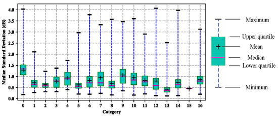
In the experiment, we used 33 multi-temporal images that operated on beam S3 in Houston and classified them into 17 categories of slices that were based on the method mentioned in Section 2.2. The classification result of the identical slices is shown in Figure 5. For each slice, we calculated a median value of backscatter coefficients. For each group of identical slices, we determined the standard deviation of 33 medians. To evaluate the backscattering stability of each category, we calculated the minimum, lower quartile, median, mean, higher quartile, and maximum of all the standard deviations of the same category. These values are shown as a box plot in Figure 6.

The quantities of categories 1, 3, 4, 7, 9, and 15 are too small; these categories have not been included in the analysis because conclusions that are based on them are not representative in the statistical sense. Among the remaining 11 categories, the box of the 13th category named “Urban and built-up” (hereinafter “urban areas”) was the flattest with the lowest position; this indicated that the median standard deviations of the identical slices in urban areas were concentrated on a smaller value, and their average was 0.42 dB. Some types of vegetation cover, such as the 14th category of cropland/natural vegetation mosaic, the 12th type of croplands, and the 10th type of grasslands, have certain growth cycles. Therefore, different growth stages and different water contents can lead to large changes in their backscatter coefficients with changing seasons. However, artificial objects, such as buildings, roads, and bridges in urban areas are not so easily influenced by the season as natural objects; thus, their backscatter coefficients are relatively more stable over time. Therefore, we selected urban areas as a stable ground category.

3.2. Extracting the Stable Backscattering Feature Using Synthetic Aperture Radar (SAR) Images

Although urban areas’ backscattering was generally stable, we could see from Figure 6 that the median standard deviations of identical slices in urban areas ranged from 0.1 dB to 2.5 dB, that is, stable or unstable differences were still present among the slices of urban areas. In order to figure out the spatial distribution of the stable or unstable urban slices, we drew the median standard deviations of all the groups of identical slices in urban areas, as Figure 7 shows. We can see that the image brightness of the stable slices is overall uniform with a few strong scattering points. The corresponding actual objects are mainly low residential areas having similar heights and shapes. Unstable slices behave very brightly in the images, and the corresponding actual objects are mainly downtown areas and buildings having very different heights and shapes.

Since there were obvious differences in the stable and unstable SAR images, we used a two-class classification model to finely filter the urban slices—the unstable ones were filtered out, and the stable ones were chosen. We determined the positive and negative samples by using a threshold of the median standard deviation of the identical slices. Figure 7 shows that 0.3 dB is a suitable threshold to distinguish two kinds of SAR image slices. Therefore, positive samples were those identical slices whose median standard deviations were less than or equal to 0.3 dB, whereas the negative samples were those whose median standard deviations were greater than 0.3 dB. Figure 8 shows some examples of positive and negative slices. To evaluate the model’s classification performance, recall ratio, and precision ratio were used; they were calculated as follows:

$$recall=\frac{TP}{TP+FN}, precision=\frac{TP}{TP+FP}$$

(2)

where $TP$, $FN$, and $FP$ are, respectively, the number of times that the model identified the positive samples as positive, the positive samples as negative, and the negative samples as positive. A higher recall ratio indicates that the model can classify more positive slices as positive ones; a higher precision ratio indicates that more slices of those that are classified as positive by the model are actually positive.

We randomly chose 15 SAR images in Houston (S3) as the training set and the other 18 images were the test set, with each image containing 9826 slices of urban areas. We used a full-connected neural network (FNN) as the classification model (as shown in Figure 9). The input was the urban slice’s image intensity. To make pre-calibrated images and after-calibrated images equivalent to the model, the inputs were preprocessed by converting to the decibel form and then reducing the average level, since the after-calibrated images differ by only a calibration constant from pre-calibrated images, according to the Equation (3):

$${\sigma }^0=DN+K$$

(3)

where ${\sigma }^0$ is the backscatter coefficient; $DN$ is the image intensity after internal calibration, antenna pattern correction, and slant range normalization; and, $K$ is the absolute calibration constant; all variables are in decibels.

Testing on 18 Houston (S3) images, the FNN model obtained an average recall ratio of 97.98% and an average precision of 80.39%. Figure 10 draws the histogram of the median standard deviations of the identical slices before and after filtering. We could see that almost all of the positive samples were identified as positive, and only a few of those slices identified as positive were actually negative. Therefore, the FNN model has good filtering ability, which also indicates that the two classes divided by 0.3 dB are separable.

However, when the model trained by Houston (S3) images was applied on Houston (S6) and Chicago (S4) datasets, the filtering performance got worse. From

Table 2. The performance of the FNN model.

		Houston (S3)	Houston (S6)	Chicago (S4) 3
Before filtering	Number of slices	9826	6809	4296
Acutal value 1	Number of slices	2526	2417	2
After SAR-model filtering	Recall ratio (%)	97.98	39.50	−
	Precision ratio (%)	80.39	59.02	−
	Number of slices 2	~3050	~1619	~1128

¹ Actual value is calculated by those actually positive slices. ² Number of slices indicates the number of urban slices that are extracted by model in each image. Because the numbers of extracted slices in different image are distinct, we give an average value. ³ For each image of Chicago (S4), there are only two positive samples; therefore, the recall and the precision ratios are not shown in the table.

, it could be seen that the precision recall of Houston (S6) was only 59.02%. For Chicago (S4) dataset, there were only two actually positive samples, but the model classified about 1128 slices as positive ones, indicating that the model had poor classification ability on this dataset. The model that was trained by S3 dataset has bad generalization ability on datasets from other beam or other city. One possible reason is that the resolution of images that were used in this study is not high enough and the ability of SAR images to express information is relatively weaker than that of optical images. Thus in next section, we proposed a method that used both SAR and optical images to finely filter the urban slices.

3.3. Extracting the Stable Backscattering Feature Using the Combination of Synthetic Aperture Radar (SAR) and Optical Images

Optical images have better information expression ability; therefore, they were added to the classification model to achieve better filtering performance. The features that were extracted from the optical and SAR images were different in the physical sense. Thus, they were used to train two separate models. Then, the results of these two models were combined by voting to produce the final classification result, that is, the final result was positive only when the results of both models were positive. Since the SAR model has been described in Section 3.2, we introduced how to train an optical model in this section.

Firstly the optical image slices of urban areas should be obtained. We used the software named BIGEMAP (Chengdu BIGEMAP Data Processing Co., Ltd., Chengdu, China, version 20.0.0) to crop the optical images in Houston and Chicago from Google Earth, with a resolution of 4.78 m. Then, the urban slices were extracted from these images using the method that was mentioned in Section 2.2. Since a group of identical slices in the SAR images corresponded to the same slice in the optical image, the quantity of optical slices that could be used to train the model were much smaller than that of SAR slices. There were only 9826, 6809, and 4296 optical slices of Houston (S3), Houston (S6), and Chicago (S4) datasets, respectively. Since the quantity of the optical slices was small, we used a pre-trained CNN model named SqueezeNet as the optical classification model and used the optical slices in Houston (S3) to fine-tune the model. SqueezeNet is a small deep learning neural network structure (see Figure 11); it can achieve the accuracy that is comparable to AlexNet with 50 times fewer parameters [22].

The weights of the pre-trained SqueezeNet model were downloaded from Github (https://github.com/rcmalli/keras-squeezenet/releases). We used 80% of the optical slices of Houston (S3) dataset as the training set and 20% as the validation set. After fine-tuning, SqueezeNet achieved 86% and 85% accuracy on training and validation set, respectively. The filtering performance of optical model on three datasets is shown in

Table 3. The performance of optical model.

	Houston (S3)	Houston (S6)	Chicago (S4)
Recall ratio (%)	64.41	39.02	−
Precision ratio (%)	76.85	86.83	−
Number of slices	2117	1086	320

. When compared to the SAR model, the optical model improved the precision ratio of the Houston (S6) dataset and classified less slices of the Chicago (S4) dataset as positive. However, the recall and precision ratio on Houston (S3) got lower. In order to utilize the advantages of two models, we combined their classification results by voting. The performance of the combined model is shown in

Table 4. The performance of the combined model.

	Houston (S3)	Houston (S6)	Chicago (S4)
Recall ratio (%)	63.13	20.49	−
Precision ratio (%)	96.40	90.16	−
Number of slices	~1659	~549	~131

. We could see that, when compared with the SAR model and the optical model, the combined model increased the precision ratio at the expense of the reduction of recall ratio, both for Houston (S3) and Houston (S6) datasets. Since the purpose of filtering is to obtain stable urban slices and then use them to extract stable feature, the precision ratio is more important than recall ratio. In this sense, the combined model performed well, with the precision ratios of 96.40% and 90.16% on two Houston datasets. For Chicago, there were only 131 slices extracted, which was in line with the reality. Therefore, we can use this combined model to classify all of the urban slices; then, select the positive samples and only use them to extract stable backscattering feature.

In order to clarify how the spatial distribution of urban slices changes after combined model filtering, we draw the figures as below. When compared with all urban slices in Figure 12a, the stable urban slices in Figure 12b,c correspond to those areas where the image brightness is not very strong. In addition, the stable slices that were extracted by the model (see Figure 12c) are similar to the actually stable slices (see Figure 12b) in the terms of spatial distribution. Therefore, the stable slices after combined model filtering are still representative to estimate the calibration constant.

4. Results and Validation

4.1. Stability of the Extracted Feature

Through the above analysis, we knew that urban areas had good temporal stability compared to other categories. Thus, we considered the average of all medians of slices in urban areas as a stable backscattering feature (hereinafter “median center”). Therefore, identical slices were only used in the measurement of temporal stability, but not in the final calibration process, which reduced the demand for the accuracy of geographical registration. In Figure 13, each curve represents the distribution of all urban slices’ medians in the same image. We could see that all of the centers of curves were very close although each curve spread a wide range (−1 dB~−10 dB), which also proved that the median center could be used as a stable feature.

For each image, a median center of all urban slices can be calculated. For a set of images, we can compute an average and a standard deviation of all median centers, as shown in

Table 5. The stability of median centers (before filtering).

	Houston (S3)	Houston (S6)	Chicago (S4)
Average/dB	−5.90	−6.97	−7.94
Standard deviation/dB	0.31	0.27	0.52

. The curves in Figure 14 depict how the median centers vary as time changes. The standard deviations of median centers of S3, S6, and S4 datasets were 0.31 dB, 0.27 dB, and 0.52 dB, respectively. All of these have good temporal stability, especially the datasets in Houston. The precipitation in Chicago varies at a higher degree with time changes than that in Houston; this may be one of the reasons that urban areas in Chicago perform worse on stability.

However, when compared with the existing calibrators’ radiometric accuracy, the stability of urban areas must be further improved. In Section 3.2, we introduced the method of finely filtering the urban slices with SAR images. Then, we only took those urban slices that were classified as positive by the model into account and used them to calculate the median center. The stability of median centers after SAR model filtering is shown in

Table 6. The stability of median centers (after synthetic aperture radar (SAR) model filtering).

		Houston (S3)	Houston (S6)	Chicago (S4)
Actual value	Average/dB	−5.57	−7.62	−7.49
	Standard deviation/dB	0.19	0.18	0.28
After SAR model filtering	Average/dB	−5.72	−7.45	−7.64
	Standard deviation/dB	0.21	0.23	0.53

and Figure 15. The standard deviation of the median center of Houston (S3) dataset was reduced from 0.31 dB to 0.21 dB, that is, the median center got more stable after filtering. But, for Houston (S6) and Chicago (S4) datasets, due to the bad generalization ability of the model that was trained by SAR images, the stability of their median centers had not been improved significantly or even got worse.

While considering the good classification ability of the combined model in Section 3.3, we used those urban slices that were identified as positive by the combined model to calculate the median center; the results are shown in

Table 7. The stability of median centers (after the combined model filtering).

	Houston (S3)	Houston (S6)	Chicago (S4)
Average/dB	−5.57	−7.41	−7.12
Standard deviation/dB	0.19	0.19	0.45

. It could be seen that the stabilities of median center of S3, S6 and S4 datasets after filtering were 0.19 dB, 0.19 dB, and 0.45 dB, respectively. When compared with the results before filtering (in Table 5) and the results after SAR model filtering (in Table 6), the stability of median center after combined model filtering had been obviously improved. Particularly, the result of Houston (S3) dataset was quite ideal; its median centers were almost identical to that of the actually stable slices (see Figure 16). Furthermore, the stabilities of both datasets in Houston reached the level of the actual value. Although the result in Chicago could not be compared with the actual value (since it was computed by only two actual positive slices), the stability of the median center after combined filtering got more stable than that before filtering. Therefore, this model not only promotes the performance on the dataset from the same city and the same beam with the training set, but it also improves the ability to generalize on datasets from other cities or beams.

After filtering by the combined model, the temporal stability of the median center in the urban areas has been further improved. Finally, we extracted a backscattering feature (median center) in urban areas with the temporal stability of 0.19 dB in Houston and 0.45 dB in Chicago. This result shows that there are differences in the backscattering stability of urban areas in different cities, which may be related to various factors, such as the distribution form of buildings or the ratio of artificial targets and natural objects.

4.2. Validation of the Stability

Through the analysis of ground objects’ backscattering characteristics, we extracted the median center of urban areas with a temporal stability of 0.19 dB. In order to determine whether this feature could be used for long-term system monitoring, we compared its stability with the Amazon rainforest, a natural target that has long been considered uniform and stable. Finally, we proposed a calibration scheme that is based on the stability of this feature and tested its accuracy.

4.2.1. Comparison with the Rainforest

Because the ${\sigma }^0$ of rainforest at C-band follows a cosine law as the incidence angle changes, its ${\gamma }^0$ is almost independent on the incidence angle, as Equation (4) depicts [23]:

$${\gamma }^0\left(\theta \right)=\frac{{\sigma }^0\left(\theta \right)}{\cos \left(\theta \right)}$$

(4)

where $\theta$ is the incidence angle. Therefore, ${\gamma }^0$ is usually used as the description of rainforest’s backscattering coefficient to avoid the impact of incidence angle.

The rainforest dataset consisted of 64 images ranging from 64.15°W to 72.61°W and from 3.46°S to 11.74°S. These images were collected during the period from October 2014 to August 2016, with six different strip mode beams. The mean levels of ${\gamma }^0$ ranged from approximately −6.5 dB to −5 dB with a standard deviation of 0.46 dB. In particular, the ascending orbit and the descending orbit are performed in the evening and morning at the Amazon, respectively, which causes a difference of vegetation water content and affects the backscattering level. Therefore, this dataset was further analyzed by distinguishing the orbit direction, as shown in Figure 17. As a result, the mean ${\gamma }^0$ from the ascending and descending orbit were present at the mean level of −6.05 dB and −5.74 dB, respectively, and the standard deviation in the ascending orbit mode (0.37 dB) was lower than that in the descending one (0.49 dB). Therefore, we can conclude that the median center of ${\sigma }^0$ in urban areas is more stable than the mean ${\gamma }^0$ of rainforests, and it can be used as a stable calibration reference.

4.2.2. Calibration Scheme Using the Stable Feature

Using the stability of the median center in filtered urban areas, we presented an estimation scheme of the calibration constant, as shown in Figure 18. If there are several calibrated multi-temporal images from the same beam in a certain city, their corresponding optical images can be available from Google Earth. Then, the SAR and the optical image slices in urban areas can be extracted using the MODIS products, which can train a SAR-model and an optical-model. After these two models are combined by voting, we can use the combined model to filter urban slices from these training images, and obtain the median center ($Me{d}_{ref}$) calculated by all of the positive slices. For an image to be calibrated, we can extract its SAR and optical urban slices, and then input them into the classification model. Subsequently, the SAR images of those slices that are identified as positive are involved to calculate the median center ($Me{d}_{org}$). Finally, the calibration constant $K$ of this image can be calculated, as follows:

$$K=Me{d}_{ref}-Me{d}_{org}$$

(5)

where all of the variables are in decibels. This scheme can be used to monitor the calibration constant after the system is absolutely calibrated by the traditional methods, such as corner reflectors and transponders. It uses accumulated images to obtain the reference value of the median center in urban areas and then take advantage of this feature’s temporal stability to estimate the calibration constant of the newly acquired images. Therefore, this scheme can monitor the calibration constant’s changes over time.

In particular, due to the bias of the median center’s average levels between different datasets, this scheme can only be used to monitor the absolute calibration constant for images from the same beam and the same city with the training set. For images from other beams or cities, it can only be used to conduct relatively radiometric calibration; however, once several absolutely calibrated images are available, all of the images’ calibration constants can be estimated.

The estimated RMSEs of the calibration constant that was validated by 18 Houston (S3) images, 34 Houston (S6) images, and 31 Chicago (S4) images were 0.17 dB, 0.21 dB, and 0.47 dB, respectively. For the S6 and S4 dataset, we assumed that the first three images were calibrated, and then used the average of their median centers as a reference.

From Figure 19, we could see that the model trained by 15 SAR images and one optical image in Houston (S3) performed well on the other 18 images in Houston (S3) and 34 images in Houston (S6), but got relatively worse on 31 images in Chicago (S4). This is because the median center of urban slices in Houston is stable, both on beam S3 and beam S6, but it behaves less stable in Chicago. The performance of this scheme in different cities depends on the stability of the city itself.

5. Discussion

Since it is difficult for exiting methods to monitor the absolute calibration constant continuously, we need to find a stable backscattering feature in common scenes and use it as a calibration reference. In this paper, we proposed a method of analyzing and exacting the stable backscattering feature, and finally determined that the median center of backscatter coefficients in urban areas is a stable feature with a temporal standard deviation of 0.19 dB. A contrast experiment suggests that this feature is even more stable than the ${\gamma }^0$ of the Amazon rainforest. Then, we provided a scheme of calculating the calibration constant using this feature. The estimation errors were within 0.5 dB when it was tested by three datasets.

Different from those distributed targets that are concentrated in a specific area, urban areas are dispersedly distributed in common imaging scenes. Therefore, the radar can easily obtain urban images while completing the normal observation tasks and monitor the calibration constant from these images without the regional restriction of calibration field. Thus, it can increase the measurement frequency of the constant and is then beneficial for improving the accuracy of the calibration constant. Furthermore, this feature has a better temporal stability than the distributed targets.

When compared with the method based on PSs, this scheme reduces the demanding for registration, although these two methods have similar estimated accuracy. The PSs-based method needs lots of long-term and coherent PSs in the imaging scenes, whereas the feature used in this scheme is the statistical median center of urban slices, which is more fault-tolerant, and therefore is simpler to implement.

Nevertheless, there are still several problems. The stability analysis requires multi-temporal images from the same city, so we used only two cities for analysis and validation due to the lack of data. Verification experiments on other cities need to be conducted to draw a more general conclusion. Despite this, the difference in backscattering stability between these two cities is still obvious, as we find that the stability of urban areas in Houston is 0.19 dB but 0.45 dB in Chicago. Further studies should be carried out to figure out the reasons, such as the influence of the precipitation, and then eliminate the differences. The SAR images that are used in this paper have a relatively low resolution, which affects the classification results of the model. If there are images with higher resolution available, then the filtering performance may be better.

6. Conclusions

We analyzed the stability of C-band backscattering using a ${\sigma }^0$ sample database and determined that the median center of the backscatter coefficients in urban areas would be a statistically stable feature. After finely filtering by a classification model based on neural networks, the temporal standard deviation of this feature can be as low as 0.19 dB. Finally, we proposed a calibration constant monitoring scheme using this feature and achieved good results on a dataset from different cities and beams, with the estimated RMSEs within 0.5 dB. Therefore, urban areas can be used as a viable calibration reference to be further studied and applied.

References

1. Pulvirenti, L.; Squicciarino, G.; Cenci, L.; Boni, G.; Pierdicca, N.; Chini, M.; Versace, C.; Campanella, P. A surface soil moisture mapping service at national (Italian) scale based on Sentinel-1 data. Environ. Model. Softw. 2018, 102, 13–28. [Google Scholar] [CrossRef]
2. Koyama, C.N.; Sato, M. Soil moisture and biomass retrieval using ALOS/PALSAR data. In Proceedings of the 2013 Asia-Pacific Conference on Synthetic Aperture Radar (APSAR), Tsukuba, Japan, 23–27 September 2013. [Google Scholar]
3. Huang, W.; Liu, X.; Gill, E.W. Ocean Wind and Wave Measurements Using X-Band Marine Radar: A Comprehensive Review. Remote Sens. 2017, 9, 1261. [Google Scholar] [CrossRef]
4. Pichierri, M.; Hajnsek, I.; Zwieback, S.; Rabusa, B. On the potential of Polarimetric SAR Interferometry to characterize the biomass, moisture and structure of agricultural crops at L-, C- and X-Bands. Remote Sens. Environ. 2018, 204, 596–616. [Google Scholar] [CrossRef]
5. Guccione, P.; Scagliola, M.; Giudici, D. Low-Frequency SAR Radiometric Calibration and Antenna Pattern Estimation by Using Stable Point Targets. IEEE Trans. Geosci. Remote Sens. 2018, 56, 635–646. [Google Scholar] [CrossRef]
6. Giudici, D.; Villa, A.; Recchia, L.; Guarnieri, A.M.; Johnsen, H.; Meadows, P.; Mouche, A.; Miranda, N.; Ottavianelli, G. Long Term PS-CAL analysis of ERS and ASAR data and comparison to other calibration techniques. In Proceedings of the 10th European Conference on Synthetic Aperture Radar, Berlin, Germany, 3–5 June 2014. [Google Scholar]
7. Reimann, J.; Schwerdt, M.; Schmidt, K.; Ramon, N.T.; Castellanos, G.A.; Döring, B.; Rudolf, D.; Raab, S.; Antony, J.M.W.; Zink, M. The DLR SAR calibration center. In Proceedings of the 5th Asia-Pacific Conference on Synthetic Aperture Radar (APSAR), Singapore, 1–4 September 2015. [Google Scholar]
8. Birrer, I.J.; Bracalente, E.M.; Dome, G.J.; Sweet, J.; Berthold, G. σ signature of the Amazon rain forest obtained from the SeaSat scatterometer. IEEE Trans. Geosci. Remote Sens. 1982, GE-20, 11–17. [Google Scholar] [CrossRef]
9. Bhowmick, S.A.; Kumar, R.; Kumar, A.S.K. Cross Calibration of the OceanSAT -2 Scatterometer with QuikSCAT Scatterometer Using Natural Terrestrial Targets. IEEE Trans. Geosci. Remote Sens. 2014, 52, 3393–3398. [Google Scholar] [CrossRef]
10. Hawkins, R.; Attema, E.; Crapolicchio, R.; Lecomte, P.; Closa, J.; Meadows, P.; Srivastava, S. Stability of Amazon Backscatter at C-Band: Spaceborne Results from ERS-1/2 and RADARSAT-1. In Proceedings of the CEOS SAR Workshop, Toulouse, France, 26–29 October 1999. [Google Scholar]
11. Luscombe, A.P. Radiometric calibration information from RADARSAT-1 Amazon measurements. In Proceedings of the 2001 CEOS SAR Workshop, Tokyo, Japan, 2–5 April 2001. [Google Scholar]
12. Ridley, J.; Strawbridge, F.; Card, R.; Phillips, H. Radar backscatter characteristics of a desert surface. Remote Sens. Environ. 1996, 57, 63–78. [Google Scholar] [CrossRef]
13. Horstmann, J.; Lehner, S. A new method for radiometric calibration of spaceborne SAR and its global monitoring. In Proceedings of the IEEE International Geoscience and Remote Sensing Symposium, Toronto, ON, Canada, 24–28 June 2002. [Google Scholar]
14. D’Aria, D.; Ferretti, A.; Monti Guarnieri, A.; Tebaldini, S. SAR Calibration Aided by Permanent Scatterers. IEEE Trans. Geosci. Remote Sens. 2010, 48, 2076–2086. [Google Scholar] [CrossRef]
15. Iannini, L.; Monti Guarnieri, A. A PS-based approach for the callibration of spaceborne polarimetric SAR systems. In Proceedings of the 2012 IEEE International Geoscience and Remote Sensing Symposium, Munich, Germany, 22–27 July 2012. [Google Scholar]
16. Rizzoli, P.; Giudici, D.; D’Aria, D. Permanent Scatterers for SAR sensor Calibration. In Proceedings of the 7th European Conference on Synthetic Aperture Radar, Friedrichshafen, Germany, 2–5 June 2008. [Google Scholar]
17. Yang, J.; Qiu, X.; Ding, C.; Lei, B.; Lu, X. A Method of Analyzing and Extracting Stable Feature of Targets Backscattering for C-band SAR. J. Univ. Chin. Acad. Sci. 2018, accepted. [Google Scholar]
18. Schwerdt, M.; Schmidt, K.; Ramon, N.T.; Alfonzo, G.C.; Döring, B.J.; Zink, M.; Prats-Iraola, P. Independent Verification of the Sentinel-1A System Calibration. IEEE J. Sel. Top. Appl. Earth Obs. Remote Sens. 2016, 9, 994–1007. [Google Scholar] [CrossRef]
19. Schwerdt, M.; Schmidt, K.; Tous Ramon, N.; Klenk, P.; Yague-Martinez, N.; Prats-Iraola, P.; Zink, M.; Geudtner, D. Independent System Calibration of Sentinel-1B. Remote Sens. 2017, 9, 511. [Google Scholar] [CrossRef]
20. NASA LP DAAC. Combined MODIS, version 5.1 ed; NASA EOSDIS Land Processes DAAC, USGS Earth Resources Observation and Science (EROS) Center: Sioux Falls, SD, USA. Available online: https://lpdaac.usgs.gov (accessed on 1 January 2013).
21. Friedl, M.A.; Sulla-Menashe, D.; Tan, B.; Schneider, A.; Ramankutty, N.; Sibley, A.; Huang, X. MODIS Collection 5 global land cover: Algorithm refinements and characterization of new datasets. Remote Sens. Environ. 2010, 114, 168–182. [Google Scholar] [CrossRef]
22. Iandola, F.N.; Han, S.; Moskewicz, M.W.; Ashraf, K.; Dally, W.J.; Keutzer, K. SqueezeNet: AlexNet-level accuracy with 50x fewer parameters and <0.5 MB model size. arXiv, 2016; arXiv:1602.07360. [Google Scholar]
23. Bamler, R. Principles of synthetic aperture radar. Surv. Geophys. 2000, 21, 147–157. [Google Scholar] [CrossRef]
Figure 1. Imaging location. (a) Houston (S3 and S6 beam); and, (b) Chicago (S4 beam).
Remotesensing 10 01010 g001
Figure 2. The diagram block of classification method based on moderate-resolution imaging spectroradiometer (MODIS) Land Cover Type product (MCD12Q1).
Remotesensing 10 01010 g002
Figure 3. The block diagram of the analysis method.
Remotesensing 10 01010 g003
Figure 4. Identical slices.
Remotesensing 10 01010 g004
Figure 5. Classification result of identical slices [20].
Remotesensing 10 01010 g005
Figure 6. Temporal stability of 17 categories of ground objects. The position along the vertical axis represents the overall stability of a certain category, whereas the density reflects the concentrated degree of the stability.
Remotesensing 10 01010 g006
Figure 7. The median standard deviations of all groups of identical slices in urban areas.
Remotesensing 10 01010 g007
Figure 8. The corresponding optical images of positive and negative slices. (a) Positive; and (b) Negative. Images were cropped from Google Earth with a resolution of 4.78 m.
Remotesensing 10 01010 g008
Figure 9. The structure of full-connected neural network (FNN) model.
Remotesensing 10 01010 g009
Figure 10. The histogram of the standard deviations of the identical slices in urban areas.
Remotesensing 10 01010 g010
Figure 11. The structure of SqueezeNet [22]. Fire is a key module in SqueezeNet that reduces the numbers of parameters effectively.
Remotesensing 10 01010 g011
Figure 12. The spatial distribution of (a) all urban slices before filtering (yellow), (b) actually stable slices (cyan), and (c) the stable urban slices extracted by the combined model (purple).
Remotesensing 10 01010 g012
Figure 13. The distribution curves of urban medians in 33 images.
Remotesensing 10 01010 g013
Figure 14. The median center trends over time (before filtering).
Remotesensing 10 01010 g014
Figure 15. The median center trends over time (after SAR model filtering). (a) Houston (S3); (b) Houston (S6); and (c) Chicago (S4).
Remotesensing 10 01010 g015
Figure 16. The median center trends over time (after combined model filtering). (a) Houston (S3); (b) Houston (S6); and, (c) Chicago (S4).
Remotesensing 10 01010 g016aRemotesensing 10 01010 g016b
Figure 17. The stability of Amazon rainforests. (a) The dataset in ascending orbit; and (b) The dataset in descending orbit.
Remotesensing 10 01010 g017
Figure 18. Calibration constant estimation scheme. The colors of lines represent the different data flows (red for training set, blue for test set).
Remotesensing 10 01010 g018
Figure 19. Estimated results of calibration constants. (a) Houston (S3); (b) Houston (S6); and (c) Chicago (S4). The annotations show the root mean square errors (RMSEs) of the estimation.
Remotesensing 10 01010 g019aRemotesensing 10 01010 g019b