CraterIDNet: An End-to-End Fully Convolutional Neural Network for Crater Detection and Identification in Remotely Sensed Planetary Images

Abstract

The detection and identification of impact craters on a planetary surface are crucially important for planetary studies and autonomous navigation. Crater detection refers to finding craters in a given image, whereas identification means to actually mapping them to particular reference craters. However, no method is available for simultaneously detecting and identifying craters with sufficient accuracy and robustness. Thus, this study proposes a novel end-to-end fully convolutional neural network (CNN), namely, CraterIDNet, which takes remotely sensed planetary images of any size as input and outputs detected crater positions, apparent diameters, and identification results. CraterIDNet comprises two pipelines, namely, crater detection pipeline (CDP) and crater identification pipeline (CIP). First, we propose a pre-trained model with high generalization performance for transfer learning. Then, anchor scale optimization and anchor density adjustment are proposed for CDP. In addition, multi-scale impact craters are detected simultaneously by using different feature maps with multi-scale receptive fields. These strategies considerably improve the detection performance of small craters. Furthermore, a grid pattern layer is proposed to generate grid patterns with rotation and scale invariance for CIP. The grid pattern integrates the distribution and scale information of nearby craters, which will remarkably improve identification robustness when combined with the CNN framework. We comprehensively evaluate CraterIDNet and present state-of-the-art crater detection and identification performance with a small network architecture (4 MB).

1. Introduction

Craters are topographic features on planetary surfaces that result from impacts with meteoroids. They are the most abundant landform on the surface of planets. Their morphology and distribution enable studies of a number of outstanding issues, such as the measurement of the relative age of planetary surface, nature of degradational processes, and regional variations in geologic material [1]. In addition, craters are ideal landmarks for autonomous spacecraft navigation [2,3]. Optical landmark navigation utilizes crater information in remotely sensed image for determining spacecraft orbits around a celestial body for close flybys and low-altitude orbiting [4]. Crater detection and identification have become key technologies in deep space exploration. All these scientific applications require crater detection and identification methods. However, craters are complex objects. Crater dimensions in an image might differ by orders of magnitude. Crater shapes may also vary depending on their interior morphologies (e.g., central peaks, peak rings, central pits, and wall terraces), level of degradation, and degree of overlap with other craters [5]. The illumination conditions also vary their appearance in images. Thus, it is difficult to find discriminant features able to correctly detect and identify the crater object in a scene. Therefore, developing a highly efficient, robust crater detection and identification algorithm is significant in planetary research and deep space exploration.

Researchers have studied crater detection and identification methods as two independent algorithms. Crater detection aims to determine whether craters exist in an image and, if so, to localize them within the image. Crater detection algorithms can be classified as unsupervised or supervised algorithm. The unsupervised methods rely on pattern recognition and template matching methods to identify crater features. In refs. [6,7], edge detection filtering and Hough transforms were used to detect craters in lunar global images obtained by the U.S. Clementine spacecraft. In refs. [8,9,10], craters in the Mars Orbiter Camera images were detected through a template matching approach; this approach produces accurate result that consists of the location and dimension of the crater. Kim et al. [11] used a combination of target edge segmentation, optimal ellipse fitting, and template matching to detect craters. High Resolution Stereo Camera (HRSC) images were used, and a minimum 70% detection ratio for small size crater was achieved. Hanak [12] applied a combination of edge detection, light source direction estimation, and crater detection filter to detect candidate craters. The method improved its robustness against false positives due to non-crater terrain features. Supervised methods use machine learning concepts to train an algorithm to detect craters and have higher accuracy than unsupervised methods. In ref. [13], a continuously scalable template matching algorithm was used to detect craters in Mars Viking Orbiter imagery, and an algorithm was trained for validation. In refs. [14,15], genetic programming is utilized to train a detection algorithm on a subset of a THEMIS IR image. The algorithm generalized well but still experienced difficulties with small craters. In ref. [16], the support vector machine (SVM) approach provided detection performance on Viking Orbiter images of Mars close to that of human labelers. In refs. [17,18], an approach is presented that automatically detected craters in HRSC images by using Haar-like features and AdaBoost classifier. The methods achieved detection F1-score of up to 86%. Convolutional neural networks (CNNs) are new techniques vastly used in computer vision with promising results. Crater detection researchers have begun to pay attention to CNN. In refs. [5,19,20], CNN was applied as a binary classifier to determine whether the input features or candidate image region belongs to the crater or background. The methods were tested in HRSC images and obtained a higher detection score than all other existing methods. Palafox et al. [21] applied five CNN architectures for different image scales that ran in parallel to detect landforms on HiRISE images from Mars Reconnaissance Orbiter; and better results were achieved compared with the SVM-based classifiers. Glaude [22] used a combination of CNN and deconvolutional layer to compute the probability of belonging to a crater class at the pixel level by utilizing remotely sensed images produced by the Lunar Reconnaissance Orbital Camera. Most of these methods only use CNN as a classifier to validate selected features or image region. Therefore, they lack the capability to detect and identify craters in a scene simultaneously by using CNNs themselves.

Once craters are detected in an image and their locations are estimated, a crater identification method can use this information to match the detected craters with respect to surface landmarks in a known database. These matches provide position estimation. The crater identification problem is actually a pattern recognition problem. Each crater is related to a unique pattern by analyzing its geometric distribution in the neighborhood, and a match can then be achieved by finding the closest pattern in the catalog. The whole objective of crater identification can be boiled down to finding the correspondence between indices of detected craters and the indices of cataloged craters. Automated crater identification problem has received less attention than crater detection. The problem of identifying craters on an asteroid was addressed in ref. [4]. Crater pairs and triples in an image were compared with crater locations in a 3D model of the asteroid until a sufficient match was found. The method was tested on real deep space mission imagery, including MGS, NEAR, and Voyager, and achieved good performance. The algorithm proposed in ref. [23] was developed for the task of precision landing and was intended to work in an area around the desired landing site at altitudes of less than 100 km. The algorithm worked by calculating the two invariants of a conic pair that described the selected crater pairs. The algorithm was tested on Mars Exploration Rover images. In ref. [12], a crater identification algorithm is proposed to provide initial navigation information in lost-in-space state that did not rely on initial vehicle navigation state knowledge. The algorithm attempted to match the detected craters to those in the crater database by examining non-dimensional parameters, such as the cosines of the angles formed by crater triangles. The method achieved 82% positive identifications on Apollo mapping camera images.

The aforementioned algorithms have solved the problems in their respective fields to some extent. However, although considerable effort has been exerted, we still do not have a unanimously accepted solution for simultaneous crater detection and identification with a highly efficient, robust, and generalized performance. Thus, we propose a novel end-to-end fully convolutional neural network for simultaneous crater detection and identification, namely, CraterIDNet, which takes remotely sensed planetary images of any size as input without any preprocessing and outputs detected crater positions, apparent diameters, and indices of the identified craters. This small-footprint model has a small network size due to its fully convolutional architecture. We initially propose a pre-trained model with a high generalization performance for transfer learning. Then, anchor scale optimization and anchor density adjustment are proposed for crater detection. In addition, multi-scale impact craters are detected simultaneously by using different feature maps with multi-scale receptive fields. These strategies considerably improve the detection performance of small craters and enable the network to detect craters with respect to a wide range of sizes. We also introduce a novel method to train crater detection pipelines (CDPs). Furthermore, a grid pattern layer is proposed to generate grid patterns with rotation and scale invariance for crater identification pipeline (CIP). The grid pattern layer integrates the distribution and scale information of nearby craters into a grayscale pattern image, which will remarkably improve identification robustness when combined with the CNN framework due to its translation invariance property. The crater identification results are directly outputted through a forward propagation; prestoring a matching crater pattern database is not needed. CraterIDNet has the advantages of high detection and identification accuracy, strong robustness, and small architecture and provides an effective solution for simultaneous detection and identification of impact craters in remotely sensed planetary images.

2. CraterIDNet

The network proposed in this study, namely, CraterIDNet, is an end-to-end fully convolutional neural network model. The entire system is a single, unified network for crater detection and identification. Figure 1 and

Table 1. CraterIDNet architecture: Filter number × Filter size (e.g., 64 × 5²), Filter stride (e.g., str 2), Pooling window size (e.g., Pool 3²), and Filter padding (e.g., pad 1).

Layer Level	Architecture	Layer Level	Architecture	Layer Level	Architecture
conv1	64 × 52, str 2	conv4_3	9 × 12	conv7_3	18 × 12
conv2	64 × 52, pad 1 Pool 32, str 2 LRN	conv5	128 × 32, pad 1	conv8	32 × 32, pad 1 Pool 32, str 2 LRN
conv3	96 × 32, pad 1	conv6	128 × 32, pad 1	conv9	64 × 32, pad 1 Pool 22, str 2
conv4	96 × 32, pad 1 Pool 32, str 2 LRN	conv7	128 × 32, pad 1	conv10	64 × 32
conv4_1	96 × 32, pad 1	conv7_1	128 × 32, pad 1	conv11	Num 1 × 22
conv4_2	6 × 12	conv7_2	12 × 12

¹ Num denotes the total number of cataloged craters.

show the network architecture.

CraterIDNet takes remotely sensed planetary images of any size as input without any preprocessing and outputs detected crater positions, apparent diameters, and indices of the identified craters. The network is composed of two pipelines, CDP and CIP. The entire system uses a fully convolutional architecture without any fully connected (FC) layer, which considerably reduces the network size. To further reduce the network size without degrading the detection and identification performance, we propose a pre-trained model for CraterIDNet initialization instead of utilizing the widely used ZF [24] or VGG [25] model. The filters in convolutional layers conv1–conv7 are initialized by this small architecture pre-trained model. Martian crater samples in different regions with different sizes, shapes, and lighting conditions are served as the training instances to improve the generalization performance of the pre-trained model. After inputting new image data into CraterIDNet, the conv4 and conv7 feature maps are then fed into two CDPs, namely, CDP1 and CDP2, to detect multi-scale impact craters simultaneously. Based on the principle in ref. [26], the CDP is composed of three convolutional layers and a target layer. These additional convolutional layers generate dense anchor boxes with a specified size and aspect ratio over the input image. Objectness region bounds and scores are then regressed for each anchor box to detect crater positions and apparent diameters. The anchor boxes are selected by novel anchor scale optimization and a density adjustment strategy to improve the detection performance of small craters. The detection results from two CDPs are integrated by the target layer and then fed into the CIP. The CIP comprises a grid pattern layer and four convolutional layers. The grid pattern layer uses the information from the previous layer to generate grid patterns with rotation and scale invariance for each candidate crater. The classification results, which are represented as the indices of the identified craters, are achieved through forward propagation.

Finally, the CraterIDNet achieves crater detection and identification through a stack of convolutional and utility layers, which result in a small model size of only approximately 4 MB.

3. Methodology

The CraterIDNet architecture is introduced in the previous section. In the present section, we introduce the methodology of CraterIDNet in three stages. Section 3.1 presents the design and dataset generation of the pre-trained model. Section 3.2 introduces the CDP architecture and proposes the anchor scale optimization and density adjustment strategy for CDP. In addition, we propose the training set creation method and 3-step alternating training method for CDP. Section 3.3 introduces the grid pattern layer, dataset generation and CIP architecture.

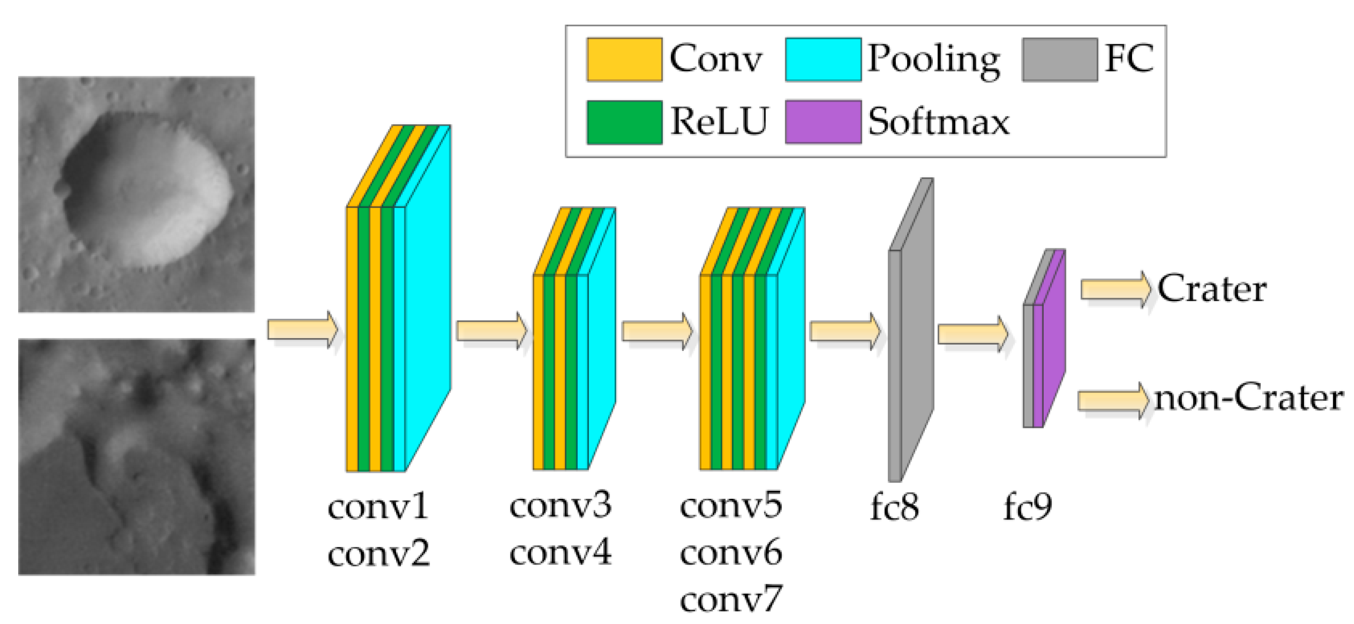
3.1. Pre-Trained Model

In practice, few people train an entire CNN from scratch (with random initialization), because having a dataset of sufficient size is relatively rare. This process will also increase the training time and sometimes even cause the network not to converge for complex tasks. Therefore, it is common to use transfer learning scenario, which is, pre-train a model and use it as an initialization or a fixed feature extractor for the task of interest. Nowadays, numerous state-of-the-art CNNs use the ZF or VGG model for transfer learning. These models perform well but their sizes are extremely large (e.g., the footprint of VGG-16 is over 500 MB). To reduce the network size and meet the needs of on-orbit missions without degrading the detection and identification performance, we use Martian crater samples in different regions with various sizes, shapes, and lighting conditions to train a small architecture pre-trained model with a high generalization performance.

3.1.1. Dataset Generation and Training Method

Five HRSC nadir panchromatic images taken by the Mars Express spacecraft in different geographical locations with different lighting conditions are selected as training scenes. These images and their attributes are shown in Figure 2 and

Table 2. Attributes of the selected scenes.

Footprint	Size (pixels)	Resolution (m/pixel)	Longitude	Latitude
h0905_0000	65,772 × 9451	12.5	49.102°W~47.128°W	13.507°N~0.363°S
h1899_0000	13,5467 × 15,543	12.5	8.533°E~12.107°E	1.462°N~27.101°S
h2956_0000	24,674 × 5567	25.0	15.181°E~17.680°E	22.462°N~12.059°N
h6456_0000	88,581 × 11,347	12.5	6.618°W~4.208°W	15.261°S~33.940°S
h6520_0000	37,964 × 7959	25.0	26.851°E~30.212°E	13.868°S~29.872°S

.

We manually catalog 1600 craters with different sizes and lighting conditions based on the Robbins Mars Crater Database [27] to serve as the initial positive samples. Then, we perform data augmentation through a combination of random rotation, shifts, and scaling to increase the diversity of the samples. Finally, a positive sample set containing 8000 instances is achieved. Subsequently, we randomly select 8000 negative samples across the scenes with non-crater geological landforms (e.g., plain, valleys, and canyons). Finally, a dataset containing 16,000 samples is generated for the pre-trained model, where the positive and negative samples have a ratio of up to 1:1.

We shuffle the dataset and split it into 10 mutually disjoint subsets. Each subset contains 1600 unique samples. Then ten-fold cross-validation is performed to evaluate the performance of the pre-trained model and aided to obtain the optimal hyperparameter settings. Thereafter, we use all the data to train the pre-trained model. Each training image is individually rescaled to 125 × 125 pixels. The training is conducted using mini-batch gradient descent with momentum. The batch size and momentum are set to 128 and 0.9, respectively. The training is regularized by weight decay and dropout regularization for the first FC layer. The L₂ penalty multiplier and dropout ratio are set to 0.0005 and 0.5, respectively. We initialize the weights for all layers using the “Xavier” method, and the biases are initialized with 0.1. The network is trained for 40 epochs with a starting learning rate of 0.01, which then decreases by a factor of 0.5 every 500 iterations.

3.1.2. Architecture

The pre-trained model serves as an initialization for the CraterIDNet model. A high performance pre-trained model will have already learned good features and effective representations of crater targets. The pre-trained model in this study uses classic CNN architecture. The input image is passed through a stack of convolutional layers. A deep net with small filters outperforms a shallow net with larger filters [25]. Therefore, we use convolutional layers with small filter size (i.e., 3 × 3 or 5 × 5). The convolutional stride of deep convolutional layers is fixed to 1 pixel; the spatial padding of these layers is 1 pixel, such that the spatial resolution is preserved after convolution. Spatial pooling is performed by three max-pooling layers, which follow some of the convolutional layers. A stack of convolutional layers is followed by two FC layers. The first FC layer has 256 channels, whereas the second performs two-way classifications (i.e., crater or non-crater) and thus contains two channels. The final layer is the soft-max layer; thus, the results can be interpreted as a probability distribution between craters and non-craters. Six groups of parameter settings of the pre-trained model are proposed with different filter sizes, number of filters and number of layers. To evaluate the performance of these architectures and identify the optimal parameter settings of the pre-trained model, ten-fold cross-validation and statistical analysis method are performed.

Table 3. Pre-trained model architectures (shown in columns). The convolutional layer parameters are denoted as “conv (filter size)-(number of channels)”. The ReLU activation function is not shown for brevity.

Model 1	Model 2	Model 3	Model 4	Model 5	Model 6
conv3-32	conv3-64	conv3-64	conv5-64	conv5-96	conv5-64
conv3-32	conv3-64	conv3-64	conv5-64	conv5-96	conv5-64
pool3	pool3	pool3	pool3	pool3	pool3
conv3-64	conv3-96	conv3-96	conv3-96	conv3-128	conv3-96
conv3-64	conv3-96	conv3-96	conv3-96	conv3-128	conv3-96
pool3	pool3	pool3	pool3	pool3	conv3-96
conv3-96	conv3-128	conv3-128	conv3-128	conv3-256	pool3
conv3-96	conv3-128	conv3-128	conv3-128	conv3-256	conv3-128
pool2	pool2	conv3-128	conv3-128	conv3-256	conv3-128
		pool2	pool2	pool2	conv3-128
					pool2
fc-256
fc-2
softmax

shows the six architectures of the pre-trained model. We perform ten-fold cross-validation utilizing the datasets generated in Section 3.1.1.

Table 4. Ten-fold cross-validation results (95% confidence interval for mean).

Model 1	Model 2	Model 3	Model 4	Model 5	Model 6
0.9636 ± 0.0041	0.9741 ± 0.0033	0.9826 ± 0.0031	0.9903 ± 0.0018	0.9918 ± 0.0008	0.9912 ± 0.0009

shows the F1-scores achieved by the six models. The depth of the models increases from the left (Model 1) to the right (Model 6). Model 6 is the deepest model, and Model 5 has the largest number of neurons. Both models achieve high performance as expected.

The selection of the optimal parameter settings is validated using one-way analysis of variance (ANOVA) parametric test. The test is performed to determine the presence of statistically significant difference between the groups. One-way ANOVA is an omnibus test that cannot identify specific groups that have statistically significant differences in their mean values. Thus, a post-hoc analysis is needed to identify the specific groups that demonstrate statistically significant difference [28]. The consolidated results of one-way ANOVA and post-hoc tests for all six models reveal that a statistically significant difference exists between these models for the F1-score metric (F = 94.608, p = 0.000). Post-hoc test further reveals that a statistically significant difference exists between Models 1, 2, and 3 and Models 4, 5, and 6. The performance of Models 4, 5, and 6 are further evaluated using one-way ANOVA. The result reveals that no statistically significant difference exists between these models for the F1-score metric (F = 1.797, p = 0.185). The statistical analysis results reveal that no significant performance gain is achieved by adding layers or neurons to Model 4. Therefore, Model 4 with a small footprint architecture is selected as the optimal parameter settings of the pre-trained model. The pre-trained model has achieved up to 99.03% mean F1-score through ten-fold cross-validation, which proves its high generalization performance. The final architecture of the pre-trained model is shown in Figure 3 and

Table 5. Pre-trained network architecture: Filter number × Filter size (e.g., 64 × 5²), Filter stride (e.g., str 2), Pooling window size (Pool 3²), and Filter padding (e.g., pad 1).

Layer Level	Architecture	Layer Level	Architecture	Layer Level	Architecture
conv1	64 × 52, str 2	conv4	96 × 32, pad 1 Pool 32, str 2 LRN	conv7	128 × 32, pad 1 Pool 22, str 2
conv2	64 × 52, pad 1 Pool 32, str 2 LRN	conv5	128 × 32, pad 1	fc8	256
conv3	96 × 32, pad 1	conv6	128 × 32, pad 1	fc9	2

.

3.2. Crater Detection Pipeline (CDP)

The CDP simultaneously regresses the objectness score and crater diameter at each location on the feature map by adding a few additional convolutional layers. This architecture is first proposed by Ren et al. [26] and named it as Region Proposal Network (RPN). The RPN starts by generating a dense grid of anchor boxes with a specified size and aspect ratio over the feature map. For each anchor, the RPN predicts a score that indicates the probability of this anchor containing an object of interest and two offsets and scale factors, which refine the location of the object. Ren et al. used anchors whose areas are 128², 256², and 512² pixels and three aspect ratios of 1:1, 1:2, and 2:1. These hyper-parameters were not carefully chosen; however, this choice of anchors delivered good results on datasets, such as VOC2007, because the objects were typically relatively large and filled a sizeable proportion of the total image area [29]. However, this architecture and anchor selection result in difficulties with crater detection. First, the RPN is only associated with the last convolutional layer whose feature and resolution are extremely weak to handle craters of various sizes. Features of small craters in the final feature map might already vanish. In addition, the detection of RPN is based on a single receptive field that cannot match different scales of craters. The intersection over union (IoU) overlap with a ground-truth box is the usual criterion by which the quality of the detection is assessed. This anchor selection is responsible for detecting relatively large objects and might fail to generate anchor boxes with sufficient IoU for small objects. Moreover, the size distribution of craters in images is not balanced. Considerably more small craters are observed than large craters. This characteristic causes the network to be sensitive to anchor selection. Improper choice of anchors will considerably degrade the recall rate of craters, which results in the poor detection performance of the network.

To solve these problems, this section presents four contributions that render the CDP accurate and efficient on crater detection: CDP architecture, optimal anchor generation strategy, CDP training set generation, and 3-step alternating training method.

3.2.1. CDP Architecture

As shown in Figure 1, CraterIDNet contains two CDPs (i.e., CDP1 and CDP2) that share early convolutional layers conv1-conv4. The anchor-associate layers (i.e., conv4_1 and conv7_1) use 3 × 3 filters. We slide these filters over the convolutional feature map. At each sliding location, n anchors are generated and mapped at the original image resolution. The feature maps outputted by the anchor-associate layers are then fed into the 1 × 1 classification convolutional layers (i.e., conv4_2 and conv7_2) and 1 × 1 regression convolutional layers (i.e., conv4_3 and conv7_3). For each anchor, the classification convolutional layer outputs two scores that estimate the probability of belonging to a crater or background class. The regression convolutional layer outputs three parameters to estimate the horizontal and vertical biases of the detected crater with respect to the center of the anchor and the ratio of the diameter of the detected crater to the width of the anchor box, respectively. The resolutions of the feature map outputted by conv4 and conv7 are approximately 1/4 and 1/8 of the original input image, respectively. In addition, the effective receptive fields of conv4 and conv7 on the input image are 37 and 101 pixels, respectively. For a crater with an apparent diameter of 12 pixels, its effective feature on conv7 feature map is only approximately 1.5 × 1.5 pixels, which is extremely weak for detection. Therefore, CDP1 associated with conv4 and CDP2 associated with conv7 are trained to detect small and large craters, respectively. This multi-scale architecture, which performs detections over multiple layers with different receptive fields, can naturally handle craters of various sizes.

The pseudo-code of CDP is shown in Algorithm 1. The classification scores and regression results are calculated through forward propagation and then fed into the target layer. Anchors whose predicted probabilities of crater are above the threshold are marked as anchor proposals. The proposal boxes are calculated based on the regression parameters. Non-maximum suppression is adopted on these proposals, and the remaining crater proposals will be outputted as the detected craters. Their centroid positions and apparent diameters are obtained as the centroids and widths of the related proposal boxes, respectively.

Algorithm 1: CDP crater detection.

input: remotely sensed image  output: detected candidate crater 1  foreach input image do 2   calculate cls and reg results through forward propagation; 3   generate anchors; 4   foreach anchor do 5    if anchor.cls > threshold then 6     proposali ← anchor.transform(anchor, reg); 7    end if 8   end for 9   proposals.sort(cls); 10    crater_proposals ← NMS(proposals, nms_threshold); 11    crater.position ← crater_proposal.center; 12    crater.diameter ← crater_proposal.width; 13    return crater 14 end for

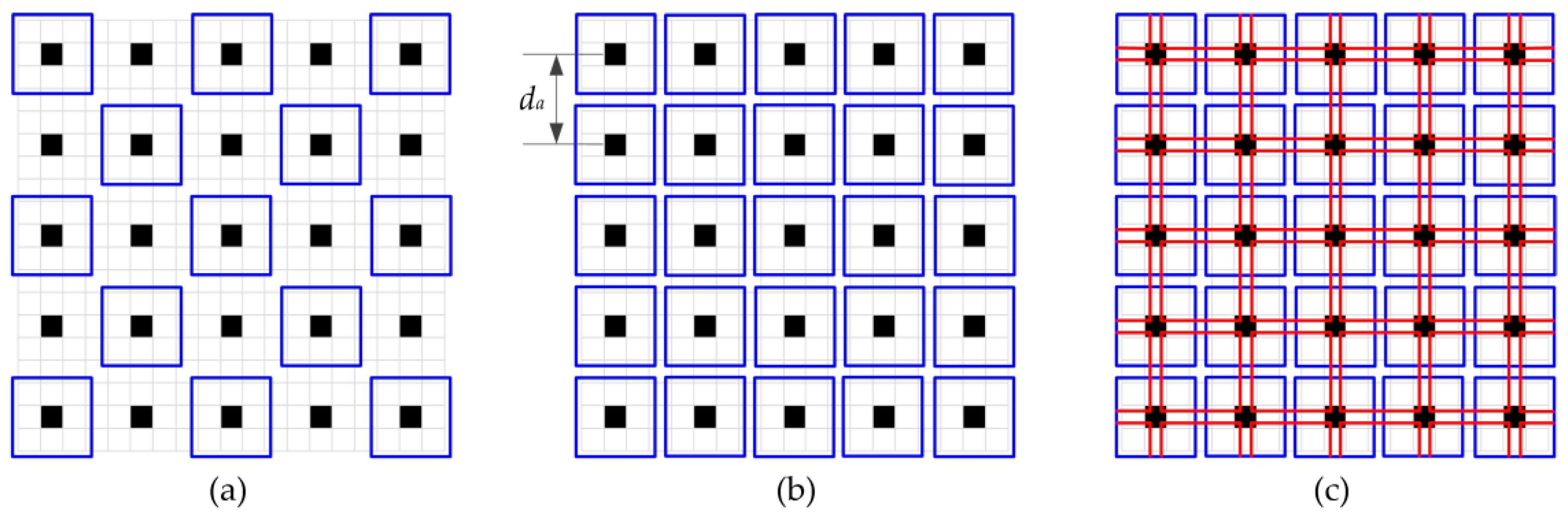
3.2.2. Optimal Anchor Generation Strategy

The optimal anchor generation strategy is performed by two steps, namely, anchor scale optimization and anchor density adjustment. Anchor selection depends on the characteristics of the dataset. Thus, we first briefly analyze the crater dataset before introducing the anchor generation strategy of CraterIDNet.

We use the Bandeira dataset [17] to generate the training and testing sets for CDPs. This dataset originates from Mars Express HRSC nadir panchromatic imagery footprint h0905_0000 and composed of six tiles (1700 × 1700 pixels each). Domain experts have labeled 3658 craters across all tiles. We select this dataset because the scene contains numerous different topographic conditions, and over half percentage of the instances occupy less than 16 × 16 pixels. This dataset is thus advantageous for creating an efficient crater detection method [22].

Table 6. Crater size distribution of the Bandeira dataset.

Size (pixels)	0~12	12~30	30~60	60~100	100~160	160~300	300~500	500~
Number	1140	2188	273	44	8	4	0	1

shows that the size distribution of the Bandeira dataset is extremely unbalanced. Only one instance is larger than 300 pixels. This instance is neglected in our dataset to avoid overfitting. Several instances, whose apparent diameters are less than 12 pixels, are difficult to distinguish in the original image, and their effective features on conv4 feature map are less than 3 × 3 pixels, which are relatively weak for detection. Therefore, instances with an apparent diameter of less than 12 pixels are neglected. Finally, a range of craters are selected in our dataset between 12 and 300 pixels.

We impose a 1:1 aspect ratio for the default anchors because the outline of the crater is approximately a circle. Eggert et al. [29] presented the relationship between anchor scale and ground-truth instance scale to classify an anchor as a positive example and the network minimum detectable object size as:

$$\sqrt{T_{IoU}}{S}_g\le S_a\le S_g/\sqrt{T_{IoU}}$$

(1)

$$S_{g\min }=\frac{d_a\left(T_{IoU}+1\right)+d_a\sqrt{2T_{IoU}(T_{IoU}+1)}}{2-2T_{IoU}}$$

(2)

where S_g is the size of the ground-truth bounding box, S_a is the size of the anchor box, T_IoU denotes the IoU threshold, and d_a is the anchor stride indicating the downsampling factor between the original image and feature map. The optimal minimum anchor size is set to S_a1, which must satisfy $S_{a1}\in \left[\sqrt{T_{IoU}}{S}_{g\min },S_{g\min }/\sqrt{T_{IoU}}\right]$, where S_gmin is the minimum size of the ground-truth instance. No ground-truth instance is smaller than S_gmin. Thus, we set S_a1 as:

$$S_{a1}=\frac{\left(1-\lambda \right)S_{g\min }}{\sqrt{T_{IoU}}}$$

(3)

Then, the detectable size range of S_a1 is [(1−λ)S_gmin, (1−λ) S_gmin/T_IoU]. The overlap ratio of the detectable object size range between anchors of neighboring scales is set as λ to ensure the reliability of crater detection on all scales in the dataset. Thus, the detectable size range of the maximum scale anchor is expressed as follows:

$$S_{gn}\in \left[\frac{{\left(1-\lambda \right)}^n{S}_{g\min }}{T_{IoU}^{n-1}},\frac{{\left(1-\lambda \right)}^n{S}_{g\min }}{T_{IoU}^n}\right]$$

(4)

The upper bound of S_gn must be larger than the maximum size of the ground-truth instance. Therefore, the optimal default anchor number must satisfy the following criterion:

$$n>\frac{\lg S_{g\max }-\lg S_{g\min }}{\lg \left(1-\lambda \right)-\lg T_{IoU}}$$

(5)

n is set as $n=\lceil \frac{\lg S_{g\max }-\lg S_{g\min }}{\lg \left(1-\lambda \right)-\lg T_{IoU}}\rceil$. Then, the optimal default anchor scales are expressed as:

$$S_{ai}=\frac{{\left(1-\lambda \right)}^i{S}_{g\min }}{T_{IoU}^{i-0.5}},i=1,\dots ,\lceil \frac{\lg S_{g\max }-\lg S_{g\min }}{\lg \left(1-\lambda \right)-\lg T_{IoU}}\rceil$$

(6)

The maximum and minimum sizes of the ground-truth instance in our dataset are S_gmax = 288 pixels and S_gmin = 12 pixels, respectively. T_IoU = 0.5 and λ = 0.1 are set at this point. Therefore, the optimal anchor number for CraterIDNet is obtained as n = 6. Considerably fewer large craters appear than small craters in the dataset. Thus, the overlap ratio λ for large-scale anchors can be slightly enlarged to increase their training opportunities. Finally, the optimal default anchor scales of CraterIDNet can be obtained using Equation (6) as 15, 27, 49, 89, 143, and 255 pixels. The anchors with scales of 15 and 27 pixels are associated with CDP1, whereas those with scales of 49, 89, 143, and 255 pixels are associated with CDP2.

In ref. [30], an anchor densification strategy is proposed for face detection. The density of the anchor is defined as the ratio of the anchor area to the anchor stride. The anchors with relatively low density are densified. However, this method does not consider the imbalance of object size distribution in a scene. The size distribution of our dataset is extremely unbalanced; thus, we propose a novel anchor density adjustment strategy to provide the anchors of each scale with approximately equal training opportunity. This strategy eliminates the imbalance of positive example for each anchor scale, which will remarkably improve the recall rate of small craters. Finally, we derive the objective function of the anchor density optimization problem, which is based on three parameters, namely, average valid anchor number (AVAN), average ground-truth instance number (AGN), and density adjustment factor (DAF).

As shown in Figure 4, an anchor is classified as a positive example when its center is in the blue region, that is:

$$IoU\left(B_g,B_a\right)\ge T_{IoU}$$

(7)

where B_g denotes the ground-truth bounding box; B_a represents the anchor box; and S_g and S_a indicate the sizes of B_g and B_a, respectively. Assume that the center of B_a is located at (x_a, y_a) and B_g is located at the origin. We ignore the cross-boundary anchors and define the valid anchor number as the total number of anchors that satisfy Equation (7) for a ground-truth instance. We define the valid anchor number when S_g = S_a as the AVAN with respect to objects within the detectable range of anchor size S_a and denoted as ${\overline{n}}_{va}$. Based on the definition of IoU, the center of a valid anchor must satisfy the following equation:

$$\left(S_a-\left|x_a\right|\right)\left(S_a-\left|y_a\right|\right)\ge T_{IoU}\left[2S_a^2-\left(S_a-\left|x_a\right|\right)\left(S_a-\left|y_a\right|\right)\right]$$

(8)

The AVAN is then approximated as the ratio of the area of a valid region (i.e., the blue region in Figure 4) to the square of the anchor stride, which can be expressed as follows:

$${\overline{n}}_{va}\approx A_{VR}/d_a^2$$

(9)

The following equation is derived based on Equations (8) and (9):

$$\begin{array}{cc}\hfill {\overline{n}}_{va}& \approx 4{\displaystyle {\int }_0^{\frac{1-T_{IoU}}{1+T_{IoU}}{S}_a}\left(S_a-\frac{2T_{IoU}{S}_a^2}{\left(1+T_{IoU}\right)\left(S_a-x_a\right)}\right)d{x}_a}/d_a^2\hfill \\ & =4\left\{\frac{1-T_{IoU}}{1+T_{IoU}}{S}_a^2+\frac{2T_{IoU}{S}_a^2}{1+T_{IoU}}\left[\ln \left(\frac{2T_{IoU}{S}_a}{1+T_{IoU}}\right)-\ln \left(S_a\right)\right]\right\}/d_a^2\end{array}$$

(10)

The total valid anchor number with respect to a selected anchor is defined as:

$${\overline{N}}_{v{a}_i}={\overline{n}}_{v{a}_i}\cdot {\overline{n}}_{g_i}$$

(11)

where ${\overline{n}}_{g_i}$ is the AGN with respect to instances within a size range of $S_{g_i}\in \left(\sqrt{T_{IoU}}{S}_{a_i},S_{a_i}/\sqrt{T_{IoU}}\right]$. Anchor density adjustment balances the total valid anchor number with respect to the anchors of each scale, such that they will obtain approximately equal training opportunities. Therefore, we propose anchor density adjustment to minimize the following squared loss function:

$$𝓁={{\displaystyle \sum _{i=1}^n\left(\frac{1}{n}-\frac{{\overline{N}}_{v{a}_i}\cdot 2^{{\tau }_i}}{{\displaystyle \sum _{i=1}^n{\overline{N}}_{v{a}_i}\cdot 2^{{\tau }_i}}}\right)}}^2$$

(12)

where τ_i is an integer and denotes the DAF with respect to each default anchor scale, and n is the number of anchors in a default anchor set. Furthermore, the number of anchors generated during training should be neither extremely large nor extremely small, which will increase the training time and degrade the recall rate, respectively. Therefore, the penalty term corresponding to the total valid anchor number is introduced, and the final objective function is expressed as follows:

$$\underset{\tau }{\tau =\arg \min }{{\displaystyle \sum _{i=1}^n\left(\frac{1}{n}-\frac{{\overline{N}}_{v{a}_i}\cdot 2^{{\tau }_i}}{{\displaystyle \sum _{i=1}^n{\overline{N}}_{v{a}_i}\cdot 2^{{\tau }_i}}}\right)}}^2+\omega \left|\frac{{\displaystyle \sum _{i=1}^n{\overline{N}}_{v{a}_i}\cdot 2^{{\tau }_i}}-N_{batch}}{N_{batch}}\right|$$

(13)

where N_batch is the mini-batch size, ω is the penalty factor, and ω = 0.02 is set at this point. By adding the penalty term, the optimization process will minimize the empirical and structural risks simultaneously. During the training process, we randomly sample N_batch anchors in an image for each iteration, where the sampled positive and negative anchors have a ratio up to 1:1. To ensure that the network generates sufficient training anchors and leave room for random selection of the anchors during training, we set the total valid anchor number generated by all default anchors as N_batch. The optimal DAF is derived based on Equation (13). When τ_i > 0, the number of corresponding anchors generated by the network is densified by a factor of $2^{{\tau }_i}$. When τ_i < 0, the number of corresponding anchors generated by the network is sparsed by a factor of $2^{{\tau }_i}$. When τ_i = 0, the number of corresponding anchors remains unchanged. The anchor density adjustments with different DAFs are shown in Figure 5, where d_a denotes the anchor stride, and the red squares indicate the added anchors.

3.2.3. Dataset Generation

The Bandeira dataset is composed of six tiles. The terrain texture in the west regions (Tiles 1_24 and 1_25) are relatively simple. The center regions (Tiles 2_24 and 2_25), which are dominated by the presence of Nanedi Valles, present the most challenging terrain for a crater detection algorithm. The east regions (Tiles 3_24 and 3_25) contain many large and overlapped craters. The CDP should be trained using ground-truth craters in various terrains of various sizes. Different testing scenes with various terrains containing craters of various sizes should be used to estimate the performance of the model on new data reliably. Therefore, six-fold cross-validation is performed to evaluate our method. Each tile takes a turn as the test scene, and the other tiles are put together to form a training scene. Two datasets associated with CDP1 and CDP2 are generated for each tile, given the unbalanced size distribution of the dataset.

The default anchor scales for CDP1 are 15 and 27 pixels. Therefore, a crater with an apparent diameter ranging from 12 to 38.2 pixels is selected for CDP1 training. Furthermore, 1000 image regions with a size of 501 × 397 pixels are randomly selected in each image tile and are randomly rotated with a probability of 50%. These image regions are then stored as image samples, and annotation files, which catalog each ground-truth crater bounding box position, are generated for each image region. The size of the ground-truth bounding box is the apparent diameter of the crater instance.

The default anchor scales for CDP2 are 49, 89, 143, and 255 pixels. Therefore, a crater with an apparent diameter ranging from 34.6 to 360.6 pixels is selected for CDP2 training. Moreover, 500 image regions with a size of 501 × 397 pixels are randomly selected in each image tile and are randomly rotated with a probability of 50%. The image regions must contain at least four craters within the size boundary and at least one crater larger than 101 pixels with a probability of 50%. These image regions are then stored as image samples, and annotation files are generated. The size of the ground-truth bounding box is the apparent diameter of the crater instance.

The statistics of crater instances in all the datasets are analyzed to achieve the AGN corresponding to each default anchor scale. Then, the optimal anchor DAF with respect to each default anchor scale is derived and shown in

Table 7. Dataset analysis result and optimal DAF.

Network	Anchor Size	AGN	AVAN	DAF
CDP1	15	16.54	3.55	1
CDP1	27	12.21	11.48	0
CDP2	49	2.88	9.46	1
CDP2	89	1.09	31.20	1
CDP2	143	0.65	80.55	0
CDP2	255	0.34	256.13	−1

, where N_batch = 256, and T_IoU = 0.5 is set at this point.

3.2.4. Three-Step Alternating Training Method

The CDP is trained end-to-end by stochastic gradient descent with momentum. We randomly sample N_batch = 256 anchors in an image to compute the loss function of a mini-batch, where the sampled positive and negative anchors have a ratio of up to 1:1. If fewer than 128 positive samples exist, then the mini-batch is padded with negative ones. The two CDPs share convolutional layers conv1–conv4; thus, we must develop a technique that allows sharing convolutional layers between the two CDPs rather than learning two separate CDPs. In this study, we propose a three-step alternating training method; the details are shown as follows.

• The pre-trained model proposed in Section 3.1 is used to initialize the convolutional layers conv1–conv7. The weights of other convolutional layers are initialized using the “Xavier” method, and biases are initialized with constant 0. The momentum and weight decay are set to 0.9 and 0.0005, respectively. The learning rates of the convolutional layers unique to CDP1 (i.e., conv4_1–conv4_3) are set to 0. Therefore, we only fine-tune conv1–conv7 and train layers unique to CDP2 by using the CDP2 dataset at this step. The network is trained for 50 epochs with a starting learning rate of 0.005 and then decreased by a factor of 0.8 every 10,000 iterations.
• The network is initialized by using the model trained in Step 1. Convolutional layers conv5–conv7 and the unique layers to CDP2 (i.e., conv7_1–conv7_3) are fixed, and the network is fine-tuned using the CDP1 dataset. The momentum and weight decay are set to 0.9 and 0.0005, respectively. The network is trained for 30 epochs with a starting learning rate of 0.001 and then decreased by a factor of 0.6 every 20,000 iterations.
• The network is initialized by applying the model trained in Step 2. The shared convolutional layers conv1–conv4 and the unique layers to CDP1 (i.e., conv4_1–conv4_3) are fixed, and the network is fine-tuned using the CDP2 dataset. The momentum and weight decay are set to 0.9 and 0.0005, respectively. The network is trained for 30 epochs with a starting learning rate of 0.0005 and then decreased by a factor of 0.8 every 15,000 iterations.

As such, both CDPs share the same convolutional layers and form a unified network.

3.3. Crater Identification Pipeline (CIP)

The output information of the CDP is fed into the CIP for crater identification based on the CraterIDNet architecture. Crater identification is similar to star identification performed in a star tracker. Typically, two databases, namely, the original crater database and the matching crater pattern database, must be prestored. The former catalogs crater index, detailed positional information, diameter, and other morphological features, whereas the latter catalogs unique feature patterns that are created for crater pattern-matching purposes. Identification is the process of searching for the unique feature pattern in the database that matches with the craters in images. The searching and matching processes are relatively time-consuming. The CIP combines the proposed grid pattern layer and the CNN framework, thereby converting the problem of searching and matching into the problem of classifying. The grid pattern layer proposed in this section generates a unique pattern image by analyzing its geometric distribution in the neighborhood for each candidate detected crater, which integrates the distribution and scale information of nearby craters into a grayscale pattern image. The pattern image is then fed into the CNN framework for classification. The output class is the corresponding index of a matched cataloged crater. Creating a matching crater pattern database is not needed, and the identification speed is improved without the searching and matching process. In addition, the combination of grid pattern layer and CNN framework allows the CraterIDNet to be robust against crater position error and apparent diameter error, which benefits from the translation invariance property of the CNN framework. This section introduces CIP from the aspects of grid pattern layer, dataset generation and CIP architecture.

3.3.1. Grid Pattern Layer

The grid pattern layer uses crater positions and apparent diameters output through the CDP as input and generates grid patterns with rotation and scale invariances. Grid algorithm is first described in ref. [31] for star identification. This algorithm generates binary grid patterns based on distribution of stars and then matches with particular patterns in the database. Based on this principle, the grid pattern layer integrates the distribution and scale information of nearby craters into a grayscale pattern image. The grid patterns are constructed as follows.

• Candidate crater selection. The altitude range for the remote sensing camera is assumed to be between H_min and H_max. H_ref is defined as the reference altitude when the training images were obtained. The craters within the detectable range at any altitude within the bounding range are selected as candidate craters. Therefore, the size of the candidate crater can be expressed as follows:

  $$D_C\in \left[\frac{D_{\min }{H}_{\max }}{H_{ref}},\frac{D_{\max }{H}_{\min }}{H_{ref}}\right]$$

  (14)

  where D_min and D_max denote the minimum and maximum apparent diameters of the candidate craters selected for identification when the crater images are acquired at altitude H_ref, respectively.
• Main crater selection. At least three craters are required within the camera field of view (FOV) to calculate the spacecraft surface relative position. We select 10 candidate craters that are closest to the center of the FOV as the main craters. If less than 10 candidate craters are found in the FOV, then all of them are selected as the main craters.
• Scale normalization. For each main crater, the distances between the main crater and its neighbor candidate craters are calculated and defined as the main distances. Let H denote the camera altitude; the main distances and apparent diameters of all candidate craters are normalized to a reference scale by a scale factor H_ref/H. The relative position of the neighbor candidate craters with respect to each main crater after scale normalization is then determined.
• Grid pattern generation. A grid of size 17 × 17 is oriented on each main crater and its closest neighboring crater. The side length of each grid cell is denoted as L_g. Each grid cell that contains at least one candidate crater is set to an active state, and its output intensity is calculated as the cumulative sum of the normalized apparent diameters of the candidate craters within this grid cell. The output intensity of the grid cells without any craters is set to 0.

Figure 6 shows the grid pattern generation process. The red and yellow circles denote the main crater and other candidate craters, respectively. Figure 6b presents the scale normalization. The blue arrow denotes the direction from the main crater to its closest neighboring candidate crater. In Figure 6c, a grid is oriented with respect to this direction. Figure 6d shows the generated grid pattern.

3.3.2. Dataset Generation and Training Method

The CIP dataset is first generated using the Bandeira crater dataset. The surface-observing instruments of Mars Express acquire their data primarily below 500-km orbit height, and the periapsis altitude of nominal Mars Express orbit is 250 km [32]; thus, we select these altitudes as the bounding altitudes (i.e., H_min = 250 km and H_max = 500 km). Let the reference altitude be the altitude when nadir panchromatic imagery footprint h0905_0000 is acquired, which is H_ref = 447.71 km. The apparent diameter of the largest detectable crater by CDP is approximately 360 pixels, and the image resolution of h0905_0000 is 12.5 m/pixel; thus, we set D_max = 4.5 km. When testing the CDP, the network has a high precision rate of relatively large craters. Most false positives (FPs) are small craters. We analyze the detection test results and set a crater size threshold T_D that ranges from 15 pixels to 30 pixels at 0.5 pixels intervals. The detection precision rate with respect to the craters larger than T_D is calculated for each T_D, and the results are shown in Figure 7.

When T_D < 18 pixels, the detection precision rate decreases sharply, which indicates that the number of FPs is considerably increased. Therefore, D_min = 18 pixels × 12.5 m/pixel = 225 m is set at this point. A total of 1008 craters with diameter in a range of D_C ∈ [251.2 m, 2.51 km] are selected as candidate craters based on Equation (14). The CIP dataset is then generated as follows.

• For each candidate crater, a unique label is provided for identification.
• The side length of the grid cell is set to L_g = 24 pixels in this study. A total of 1008 groups of grid patterns are generated for each candidate crater. Each group contains 2000 grid patterns. Crater position and apparent diameter noises are added to each candidate crater before generating grid patterns. The crater position and apparent diameter noises are random variables that follow normal distributions N(0, 2.5²) and N(1.5, 1.5²), correspondingly.
• A total of 400 grid patterns are randomly selected from each group, and the information of a neighboring crater is randomly removed to simulate the situation where the detection result of this crater is a false negative (FN).
• To simulate the situation where FPs are detected by CDP, we randomly select 700 and 400 grid patterns from each group to add one and two false craters, respectively. The false craters are added in random positions in the grid pattern, and their apparent diameters are random variables that are uniformly distributed within the range of [20, 50] pixels.
• Eight sets of grid patterns are randomly selected from each group, and each set contains 100 grid patterns. The crater information in the blue region for each set that correspond to the eight cases depicted in Figure 8 is removed to simulate the situation where the main crater is close to the boundary of the FOV.
• In total, 2,016,000 grid pattern samples are generated. The dataset is then split into 10 mutually disjoint subsets utilizing the stratified sampling method. Each subset contains the same percentage of samples of each class as the complete set (i.e., 200 samples for each candidate craters).

Ten-fold cross-validation is performed to evaluate the performance of the CIP and assist in obtaining the optimal hyperparameter settings for the CIP. Afterwards, we use all the data to train the CIP. The CIP training is performed using a mini-batch gradient descent with momentum. The batch size, momentum, and weight decay are set to 512, 0.9, and 0.0005, correspondingly. We initialize the weights of the convolutional layers of the CIP through the “Xavier” method, and the biases are initialized with 0.1. The CIP is trained for 30 epochs with a starting learning rate of 0.01, and then decreased by a factor of 0.5 every 10,000 iterations.

3.3.3. CIP Architecture

The CIP combines the proposed grid pattern layer and the CNN framework. The output detected crater information of CDP is fed into the CIP for crater identification based on the CraterIDNet architecture. The pseudo-code of CDP is shown in Algorithm 2. First, the main craters are selected by the grid pattern layer. A grid pattern image for each main crater is generated following the procedure proposed in Section 3.3.1. Second, the grid pattern images are fed into the following CNN architecture for classification. An output predicted class is an identification result, which denotes the corresponding index of a matched cataloged crater.

Algorithm 2: CIP crater identification.

input: detected craters   output: identification results 1    candidate crater selection using Equation (14); 2    foreach candidate_crater do 3   calculate distance di between crater center and image center; 4   end for 5   candidate_craters.sort(d); 6    if candidate_craters.num > 10 then 7    main_craters ← candidate_craters[:10]; 8    else 9    main_craters ← candidate_craters; 10  end if 11  iden_results = zeros(main_crater.num); 12  foreach main_crater do 13   neighbor_craters ← candidate_crater.remove(main_crater); 14   calculate main distance between main_crater and its neightbor_craters; 15   scale normalization; 16   generate grid pattern image; 17   predict class through forward propagation; 18   iden_result ← class; 19  end for

20  return iden_results

Grid pattern images with 17 × 17 pixels are generated by the grid pattern layer and then fed into the following CNN framework for classification. Convolutional layers use 3 × 3 filters. Spatial pooling is performed by using max-pooling layers with a stride of 2 pixels. The FC layer is replaced with a convolutional layer. Three groups of parameter settings of the CIP architecture are proposed with different filter numbers as listed in

Table 8. CIP architectures (shown in columns). The convolutional layer parameters are denoted as “conv (filter size)-(number of channels)”. The ReLU activation function is not shown for brevity.

Model 1	Model 2	Model 3
conv3-16	conv3-32	conv3-64
pool3	pool3	pool3
conv3-32	conv3-64	conv3-64
pool2	pool2	pool2
conv3-32	conv3-64	conv3-128
conv2-Num 1	conv2-Num 1	conv2-Num 1
softmax

¹ Num denotes the total number of cataloged craters.

. Ten-fold cross-validation with the datasets generated in Section 3.3.2 is performed to evaluate the performance of these architectures and identify the optimal parameter settings for the CIP. The identification accuracy achieved by the three models is displayed in

Table 9. Ten-fold cross-validation results (95% confidence interval for mean).

Model 1	Model 2	Model 3
0.9914 ± 0.0009	0.9974 ± 0.0007	0.9980 ± 0.0005

.

The statistical analysis method is then performed to evaluate the performance. One-way ANOVA test result shows a statistically significant difference between these models for the identification accuracy metric (F = 137.826, p = 0.000). However, the post-hoc test further reveals that no statistically significant difference occurs between Models 2 and 3 (p = 0.443). The statistical analysis results indicate that no significant performance gain is achieved by adding filters to Model 2. Therefore, Model 2 with a small footprint architecture is selected as the optimal parameter setting of the CIP. The CIP has achieved up to 99.74% mean identification accuracy through the ten-fold cross-validation, thereby confirming that the CIP has a high identification and generalization performance.

4. Experimental Results

The CraterIDNet model is obtained through the methodology discussed in Section 3. The footprint of CraterIDNet is only approximately 4 MB. In this section, experiments are performed to test and validate the crater detection and identification performance of CraterIDNet.

4.1. Validation of Crater Detection Performance

The crater detection performance of CraterIDNet is first evaluated by the cross-validation. Each tile of Bandeira dataset alternates as the test scene, and the other tiles are assembled to form a training scene. We train a model of each fold during the cross-validation and evaluate the performance of CraterIDNet using the test scene. A detected crater is labeled as true positive (TP) if it has an IoU overlap higher than 0.5 with a ground-truth crater bounding box; otherwise, the detected crater is labeled as FP. Three quality factors are used to evaluate the detection performance of CraterIDNet, that is, Precision P = TP/(TP + FP), Recall R = TP/(TP + FN), and F1-score F1 = 2PR/(P + R). The F1-score indicates the harmonic mean of the precision and recall. The cross-validation results are presented in

Table 10. Detection results achieved by CraterIDNet on each test scene.

Quality Metric	Tile 1_24	Tile 1_25	Tile 2_24	Tile 2_25	Tile 3_24	Tile 3_25	Mean
Precision	85.94%	86.26%	85.02%	83.14%	89.84%	91.02%	86.87%
Recall	95.76%	96.58%	97.31%	96.76%	95.81%	96.92%	96.52%
F1-score	90.58%	91.13%	90.75%	89.43%	92.73%	93.88%	91.42%

.

The results show that high F1-scores are achieved in all test scenes, thereby indicating that CraterIDNet has an outstanding detection performance. An average recall rate up to over 96.52% is achieved by the cross-validation, thus implying that most crater instances are correctly detected. This result will guarantee that as many TP craters as possible can participate in the identification. The precision rates are lower in the center region (Tiles 2_24, and 2_25) than in the other scenes because the terrain in the center region is complex, and several terrain textures are similar to those of crater instances. The test results of Tiles 2_25 and 3_24 are illustrated in Figure 9. Circles with the position and apparent diameter of the detected craters are depicted. The yellow, red, and blue circles denote the TP detection, FP detection, and undetected FN crater, respectively.

The test results show that most of the crater instances have been accurately detected. The false detections are mainly several terrain textures, such as basin canyon regions that are similar to those of crater instances. The smallest crater instance detected by CraterIDNet is only 9 pixels in apparent diameter, which validates the effectiveness of the CDP architecture and optimal anchor generation strategy. Thus, CraterIDNet has a high performance for detecting small craters. In Figure 9b, the largest crater in the image is undetected because this crater exceeds the detectable size limit. Figure 10 demonstrates a zoomed complex terrain of Figure 9a, which contains a densely cratered region with many overlapped craters. This region is a challenging site for any crater detection algorithm given certain overlapping geometries. In Figure 10, the overlapped craters are detected well in the densely cratered region, even for multiple overlapped craters. Therefore, CraterIDNet can effectively detect overlapped craters.

The proposed method is further evaluated by comparing the detection performance of CraterIDNet with other algorithms: Urbach [1], Bandeira [17], Ding [33], and CraterCNN [20]. We use the same dataset and test scenes as the previous methods and compare with them using the same criteria to evaluate the proposed method. These algorithms are based on similar principles. First, shape filters are used to extract highlight and shadow shapes that indicate the possible presence of craters. Crater candidates are obtained by matching the two crescent-like highlight and shadow regions and using a morphological closing operation. Second, different machine learning models (i.e., decision tree, AdaBoost, and CNN classifier) are utilized for classification of all candidates into craters and non-craters. The average F1-scores of the west region (Tile 1_24 + Tile 1_25), the center region (Tile 2_24 + Tile 2_25), and the east region (Tile 3_24 + Tile 3_25) achieved by CraterIDNet are calculated for comparison.

Table 11. Average F1-score of the different crater detection methods.

Region	Urbach	Bandeira	Ding	CraterCNN	CraterIDNet
West	67.89%	85.33%	83.89%	88.78%	90.86%
Center	69.62%	79.35%	83.02%	88.81%	90.09%
East	79.77%	86.09%	89.51%	90.29%	93.31%

displays the performance of the proposed method against results quoted from previous studies.

The previous methods lack the ability to detect small craters. Therefore, these results are obtained only by considering craters that are larger than 16 pixels. The result of CraterIDNet is obtained using all detected craters, thereby implying that all false detections are considered. The smallest crater instance detected by CraterIDNet is only 9 pixels. Approximately 40% of the FP detections are less than 16 pixels. However, CraterIDNet still outperforms the other methods with an F1-score of up to 93.31%. The results are expected to be improved if only craters larger than 16 pixels are considered.

The CNN-based CraterCNN algorithm clearly outperforms other previous methods (F1-score up to 90.29% in the east region), but is still restricted to the ability of the candidate selection algorithm. These handcrafted shape filters are not robust and minimally flexible, whereas CraterIDNet can achieve a high detection and generalization performance given its ability to learn discriminative feature filters. The previous methods have a good performance for detecting large and well-shaped craters but lack in their ability to detect small, degraded, or overlapped craters, thus resulting in a relatively low F1-score in the test scenes. In addition, CraterIDNet shows a consistent performance through these test scenes characterized by different types of terrain. The center region, which is dominated by the presence of Nanedi Valles, presents the most challenging terrain for a crater detection algorithm. The proposed method achieves an F1-score of up to 90.09% in this section, which is better than the previous methods. In addition, the previous methods can only detect irregular areas that belong to crater candidates and are incapable of directly estimating crater sizes and positions. CraterIDNet detects crater positions and estimates their apparent diameters simultaneously, thus resulting in an adaptable method. Although further tests are necessary, the performance of CraterIDNet seems sufficient for use in planetary studies and autonomous navigation.

Overall, the previous experiments verify that CraterIDNet has achieved state-of-the-art performance in crater detection.

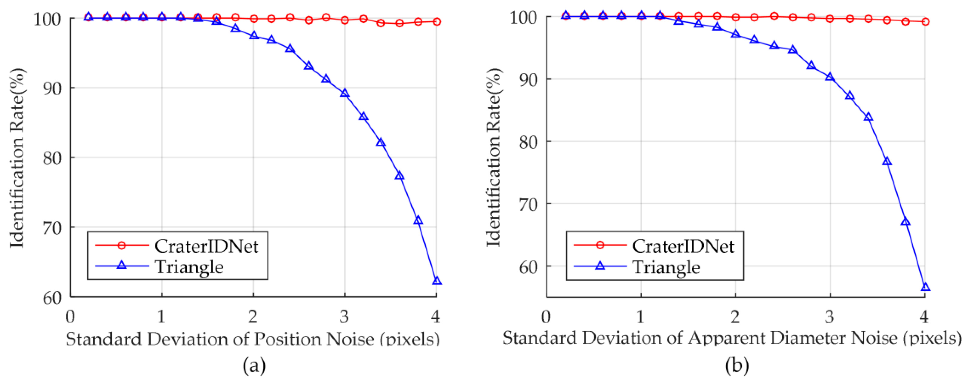
4.2. Validation of Crater Identification Performance

The crater identification performance of CraterIDNet is verified through the following comparative experiments. First, crater identification is performed by utilizing CraterIDNet and triangle matching algorithm [12], which uses actual remotely sensed planetary images. This triangle matching method aims to match the detected craters to those in the crater database by examining the angles formed by crater triangles and diameter ratios. Second, we randomly select 1000 image regions in Tile 2_25 and Tile 3_24 after rescaling the test scene by a random scale factor that is uniformly distributed within the range of [0.9, 1.4], correspondingly. The size of the selected image region is 1024 × 1024 pixels. These images are fed in CraterIDNet for detection. The detection results are used for identification using both methods. A successful identification is reported if more than four craters are correctly identified in an image region.

Table 12. Average identification rates of the two methods.

Scene	Triangle	CraterIDNet
Tile 2_25	89.3%	97.5%
Tile 3_24	94.6%	100%

presents the calculated average identification rates of the two methods in each test scene.

In Table 12, the proposed method achieves a higher identification rate. CraterIDNet achieves a 100% identification rate in Tile 3_24. The identification rate is lower in Tile 2_25 than in Tile 3_24 mainly due to the lack of impact craters in the middle canyon terrain region of Tile 2_25. The identification rate of the triangle matching algorithm is mainly affected by the false detections. The identification performance is markedly degraded when numerous FP detections occur in an image. In addition, the triangle matching algorithm is more sensitive to crater position and diameter noises than the proposed method.

A simulation experiment is performed to evaluate the robustness performance of the two methods against crater position and diameter noises. No false detections are added during the simulation. Crater position and apparent diameter noise are set as random variables that follow the normal distribution with a mean of 0 and standard deviation that ranges from 0.2 to 4 pixels at 0.2 pixel interval, thus resulting in 20 groups of noise parameters. For each set of noise parameters, crater identification is performed by applying the two methods 1000 times using a randomly selected main crater and its neighboring craters from the database after adding position and apparent diameter noises. Figure 11 exhibits the relationship between the identification rate and the standard deviation of position and apparent diameter noise.

Figure 11 illustrates that CraterIDNet can still achieve an identification rate of over 99% when the standard deviation of position and apparent diameter noise reaches 4 pixels. However, the identification rate of the triangle matching algorithm considerably decreases with the increase in the standard deviation of noises and achieves only an approximately 60% identification rate when the standard deviation of position and apparent diameter noise reaches 4 pixels. The CIP integrates the distribution and scale information of nearby craters into a grayscale pattern image. The CNN architecture of the CIP tends toward learning global patterns rather than local details, thereby making CraterIDNet very robust to crater detection errors. However, crater detection errors significantly affect the triangle matching algorithm because these errors directly affect the measured values of the parameters of the crater triangles detected in an image. If the deviation between measured and cataloged crater triangles is significantly large, then the search bounds on the parameters will change, thereby possibly resulting in a false match (i.e., match failure). The results indicate that CraterIDNet is robust against the detected crater position and apparent diameter error.

A simulation experiment is performed to evaluate the time efficiency of the two methods [34]. Crater position and apparent diameter noise are set as random variables that follow the normal distribution with a mean of 0 and a standard deviation of 1 pixel. Zero, one, two, and three false detections are added during the simulation, thus resulting in four groups of simulations. For each group of simulation, crater identification is performed by applying the two methods 10,000 times using a randomly selected main crater and its neighboring craters from the database after adding position and apparent diameter noises. The runtime of all method is recorded and averaged. The experiment is conducted on a system with a Core i7 processor and 16 GB RAM. The average identification time results of the two methods with different false detections are summarized in

Table 13. Average identification times of the two methods with different false detections (Unit: ms).

False Detection	0	1	2	3
Triangle	20.56	23.42	27.58	34.91
CraterIDNet	0.60	0.61	0.60	0.60

.

In Table 13, the average identification time of the triangle algorithm is 20.56 ms when no false detections are added, whereas that of CraterIDNet is only 0.6 ms; therefore, the proposed method is faster than the triangle algorithm. Furthermore, the identification time of the triangle algorithm increases with the false detections increasing because many false crater triangles are generated with the false detections, thereby increasing the searching and matching time. However, the time efficiency of CraterIDNet is unaffected by false detections because no searching process occurs in the CraterIDNet framework. The identification results are directly output through a forward propagation.

Furthermore, the time complexity of the CIP is expressed as $O\left(m\left(Pa+Conv+Kn\right)\right)$, whereas that of the triangle algorithms is defined as $O\left(\frac{m\left(m-1\right)\left(m-2\right)}{6}\cdot \left(Tra+N\right)\right)$. Here, m is the number of candidate craters in an image to be identified. Pa denotes the grid pattern generation time for each candidate crater. Conv is the time cost of forward propagation except for the last convolutional layer. Kn is the time cost of the last convolutional layer of the CIP during forward propagation, which is a linear function of the number of filters n of the last convolutional layer. Here, n is equal to the number of cataloged craters. Tra denotes the matching crater triangle generation time for each matching crater triangle. N is the number of cataloged crater triangles, where N is of order O(n³). Therefore, the time complexity of the CIP is achieved as O(mn), and the time complexity of the triangle algorithm is achieved as O((mn)³). Overall, CraterIDNet is quicker in terms of computation and provides better results than the triangle algorithm.

In conclusion, the experiments verify that CraterIDNet is a high-performance crater detection and identification network. CraterIDNet has a high detection and identification accuracy, strong robustness, and favorable performance for detecting small craters.

5. Conclusions

In this paper, we propose a novel end-to-end fully convolutional neural network for crater detection and identification, namely, CraterIDNet, which takes remotely sensed planetary images of any size as input without any preprocessing and outputs detected crater positions, apparent diameters, and indices of the identified craters. CraterIDNet has the advantages of high detection and identification accuracy, strong robustness, and small architecture and provides an effective solution for the simultaneous detection and identification of impact craters in remotely sensed planetary images. We first propose a pre-trained model with a high generalization performance for transfer learning. Then, anchor scale optimization and anchor density adjustment are proposed for crater detection. In addition, multi-scale impact craters are detected simultaneously by using different feature maps with multi-scale receptive fields. These strategies considerably improve the detection performance of small craters and enable the network to detect craters with respect to a wide range of sizes. We also introduce a novel method to train CDPs. Furthermore, the grid pattern layer is proposed to generate grid patterns with rotation and scale invariance for CIP. The grid pattern layer integrates the distribution and scale information of nearby craters into a grayscale pattern image, which will remarkably improve identification robustness when combined with the CNN framework due to its translation invariance property. Finally, the crater detection and identification performance of CraterIDNet is verified by experiments. The crater detection F1-score of CraterIDNet exceeds 90% in the test scene, and the smallest detected crater instance is only 9 pixels in apparent diameter. The identification rate of our proposed model exceeds 97% even in a complex terrain scene. In addition, simulation experiments indicate that CraterIDNet has a strong robustness against crater position and apparent diameter errors. CraterIDNet has achieved state-of-the-art crater detection and identification performance and provides an effective solution for the simultaneous detection and identification of impact craters in remotely sensed planetary images with a small network architecture.

References

1. Urbach, E.R.; Stepinski, T.F. Automatic detection of sub-km craters in high resolution planetary images. Planet. Space Sci. 2009, 57, 880–887. [Google Scholar] [CrossRef]
2. Riedel, J.; Bhaskaran, S.; Synnott, S.; Bollman, W.; Null, G. An Autonomous Optical Navigation and Control System for Interplanetary Exploration Missions. In Proceedings of the 2nd IAA International Conference on Lost-Cost Planetary Missions, Laurel, MD, USA, 16–19 April 1996. [Google Scholar]
3. Jun’; Kawaguchi, I.; Hashimoto, T.; Kubota, T.; Sawai, S.; Fujii, G. Autonomous optical guidance and navigation strategy around a small body. J. Guid. Control Dyn. 1997, 20, 1010–1017. [Google Scholar] [CrossRef]
4. Cheng, Y.; Johnson, A.E.; Matthies, L.H.; Olson, C.F. Optical landmark detection for spacecraft navigation. In Proceedings of the 13th Annual AAS/AIAA Space Flight Mechanics Meeting, Ponce, Puerto Rico, 9–13 February 2003; pp. 1–19. [Google Scholar]
5. Emami, E.; Bebis, G.; Nefian, A.; Fong, T. Automatic Crater Detection Using Convex Grouping and Convolutional Neural Networks. In Proceedings of the 11th International Symposium on Visual Computing, Las Vegas, NV, USA, 14–16 December 2015; pp. 213–224. [Google Scholar]
6. Leroy, B.; Medioni, G.; Johnson, E.; Matthies, L. Crater detection for autonomous landing on asteroids. Image Vis. Comput. 2001, 19, 787–792. [Google Scholar] [CrossRef]
7. Honda, R.; Iijima, Y.; Konishi, O. Mining of topographic feature from heterogeneous imagery and its application to lunar craters. In Progress in Discovery Science; Springer: Berlin, Germany, 2002; pp. 395–407. [Google Scholar]
8. Barata, T.; Alves, E.I.; Saraiva, J.; Pina, P. Automatic recognition of impact craters on the surface of Mars. In Proceedings of the International Conference Image Analysis and Recognition, Proto, Portugal, 29 September–1 October 2004; pp. 489–496. [Google Scholar]
9. Magee, M.; Chapman, C.; Dellenback, S.; Enke, B.; Merline, W.; Rigney, M. Automated identification of Martian craters using image processing. In Proceedings of the 34th Annual Lunar and Planetary Science Conference, League City, TX, USA, 17–21 March 2003. [Google Scholar]
10. Saraiva, J.; Bandeira, L.; Pina, P. A structured approach to automated crater detection. In Proceedings of the 37th Annual Lunar and Planetary Science Conference, League City, TX, USA, 13–17 March 2006. [Google Scholar]
11. Kim, J.R.; Muller, J.-P.; van Gasselt, S.; Morley, J.G.; Neukum, G. Automated crater detection, a new tool for Mars cartography and chronology. Photogramm. Eng. Remote Sens. 2005, 71, 1205–1217. [Google Scholar] [CrossRef]
12. Hanak, F.C. Lost in Low Lunar Orbit Crater Pattern Detection and Identification. Ph.D. Thesis, The University of Texas at Austin, Austin, TX, USA, May 2009. [Google Scholar]
13. Vinogradova, T.; Burl, M.; Mjolsness, E. Training of a crater detection algorithm for Mars crater imagery. In Proceedings of the IEEE Aerospace Conference, Big Sky, MT, USA, 9–16 March 2002; p. 7. [Google Scholar]
14. Plesko, C.; Brumby, S.; Asphaug, E.; Chamberlain, D.; Engel, T. Automatic crater counts on Mars. In Proceedings of the 35th Lunar and Planetary Science Conference, League City, TX, USA, 15–19 March 2004. [Google Scholar]
15. Plesko, C.; Werner, S.; Brumby, S.; Asphaug, E.; Neukum, G.; Team, H.I. A statistical analysis of automated crater counts in MOC and HRSC data. In Proceedings of the 37th Annual Lunar and Planetary Science Conference, League City, TX, USA, 13–17 March 2006. [Google Scholar]
16. Wetzler, P.G.; Honda, R.; Enke, B.; Merline, W.J.; Chapman, C.R.; Burl, M.C. Learning to detect small impact craters. In Proceedings of the IEEE Application of Computer Vision, Breckenridge, CO, USA, 5–7 January 2005; pp. 178–184. [Google Scholar]
17. Bandeira, L.; Ding, W.; Stepinski, T. Automatic detection of sub-km craters using shape and texture information. In Proceedings of the 41st Lunar and Planetary Science Conference, Woodlands, TX, USA, 1–5 March 2010; p. 1144. [Google Scholar]
18. Martins, R.; Pina, P.; Marques, J.S.; Silveira, M. Crater detection by a boosting approach. IEEE Geosci. Remote Sens. Lett. 2009, 6, 127–131. [Google Scholar] [CrossRef]
19. Cohen, J.P. Automated Crater Detection Using Machine Learning. Ph.D. Thesis, University of Massachusetts, Boston, MA, USA, May 2016. [Google Scholar]
20. Cohen, J.P.; Lo, H.Z.; Lu, T.; Ding, W. Crater detection via convolutional neural networks. In Proceedings of the 47th Lunar and Planetary Science Conference, Woodlands, TX, USA, 21–25 March 2016. [Google Scholar]
21. Palafox, L.F.; Hamilton, C.W.; Scheidt, S.P.; Alvarez, A.M. Automated detection of geological landforms on Mars using Convolutional Neural Networks. Comput. Geosci. 2017, 101, 48–56. [Google Scholar] [CrossRef] [PubMed]
22. Glaude, Q. CraterNet: A Fully Convolutional Neural Network for Lunar Crater Detection Based on Remotely Sensed Data. Master’s Thesis, University of Liège, Liège, Wallonia, Belgium, June 2017. [Google Scholar]
23. Cheng, Y.; Ansar, A. Landmark based position estimation for pinpoint landing on Mars. In Proceedings of the 2005 IEEE International Conference on Robotics and Automation, Barcelona, Spain, 18–22 April 2005; pp. 1573–1578. [Google Scholar]
24. Zeiler, M.D.; Fergus, R. Visualizing and understanding convolutional networks. In Proceedings of the 13th European Conference on Computer Vision, Zurich, Switzerland, 6–12 September 2014; pp. 818–833. [Google Scholar]
25. Simonyan, K.; Zisserman, A. Very deep convolutional networks for large-scale image recognition. In Proceedings of the International Conference on Learning Representations, San Diego, CA, USA, 7–9 May 2015. [Google Scholar]
26. Ren, S.; He, K.; Girshick, R.; Sun, J. Faster R-CNN: Towards real-time object detection with region proposal networks. IEEE Trans. Pattern Anal. Mach. Intell. 2017, 39, 1137–1149. [Google Scholar] [CrossRef] [PubMed]
27. Robbins, S.J.; Hynek, B.M. A new global database of Mars impact craters ≥1 km: 2. Global crater properties and regional variations of the simple-to-complex transition diameter. J. Geophys. Res. Planets 2012, 117. [Google Scholar] [CrossRef] [Green Version]
28. Sivaramakrishnan, R.; Antani, S.; Candemir, S.; Xue, Z.; Abuya, J.; Kohli, M.; Alderson, P.; Thoma, G. Comparing deep learning models for population screening using chest radiography. In Proceedings of the 2018 SPIE Medical Imaging, Houston, TX, USA, 10–15 February 2018; p. 105751E. [Google Scholar]
29. Eggert, C.; Zecha, D.; Brehm, S.; Lienhart, R. Improving Small Object Proposals for Company Logo Detection. In Proceedings of the 2017 ACM on International Conference on Multimedia Retrieval, Bucharest, Romania, 6–9 June 2017; pp. 167–174. [Google Scholar]
30. Zhang, S.; Zhu, X.; Lei, Z.; Shi, H.; Wang, X.; Li, S.Z. FaceBoxes: A CPU real-time face detector with high accuracy. In Proceedings of the 2017 International Joint Conference on Biometrics, Denver, CO, USA, 1–4 October 2017. [Google Scholar]
31. Padgett, C.; Kreutz-Delgado, K. A grid algorithm for autonomous star identification. IEEE Trans. Aerosp. Electron. Syst. 1997, 33, 202–213. [Google Scholar] [CrossRef]
32. Jaumann, R.; Neukum, G.; Behnke, T.; Duxbury, T.C.; Eichentopf, K.; Flohrer, J.; Gasselt, S.; Giese, B.; Gwinner, K.; Hauber, E. The high-resolution stereo camera (HRSC) experiment on Mars Express: Instrument aspects and experiment conduct from interplanetary cruise through the nominal mission. Planet. Space Sci. 2007, 55, 928–952. [Google Scholar] [CrossRef]
33. Ding, W.; Stepinski, T.F.; Mu, Y.; Bandeira, L.; Ricardo, R.; Wu, Y.; Lu, Z.; Cao, T.; Wu, X. Subkilometer crater discovery with boosting and transfer learning. ACM Trans. Intell. Syst. Technol. 2011, 2, 39. [Google Scholar] [CrossRef]
34. Senthilnath, J.; Kulkarni, S.; Benediktsson, J.A.; Yang, X.-S. A novel approach for multispectral satellite image classification based on the bat algorithm. IEEE Geosci. Remote Sens. Lett. 2016, 13, 599–603. [Google Scholar] [CrossRef]
Figure 1. Network architecture of CraterIDNet.
Remotesensing 10 01067 g001
Figure 2. Selected HRSC nadir panchromatic images.
Remotesensing 10 01067 g002
Figure 3. Architecture of the pre-trained model.
Remotesensing 10 01067 g003
Figure 4. Criterion for an anchor to be classified as a positive example.
Remotesensing 10 01067 g004
Figure 5. Anchor density adjustment: (a) τi = −1; (b) τi = 0; and (c) τi = 1.
Remotesensing 10 01067 g005
Figure 6. Grid pattern generation process: (a) candidate craters and main crater selection; (b) scale normalization; (c) orienting a grid on the main crater and its closest neighboring crater; and (d) final grid pattern generated by the grid pattern layer.
Remotesensing 10 01067 g006
Figure 7. Detection precision versus crater size threshold TD.
Remotesensing 10 01067 g007
Figure 8. Removal of crater information in the blue region to simulate the situation where the main crater is close to the boundary of the FOV.
Remotesensing 10 01067 g008
Figure 9. Crater detection test results of CraterIDNet: (a) Tile 2_25; and (b) Tile 3_24.
Remotesensing 10 01067 g009
Figure 10. Crater detection test results of CraterIDNet on a complex terrain in Tile 2_25: densely cratered terrain with many overlapped craters.
Remotesensing 10 01067 g010
Figure 11. Identification rate versus standard deviation of noise: (a) Position noise; and (b) Apparent diameter noise.
Remotesensing 10 01067 g011