Landslide Identification and Monitoring along the Jinsha River Catchment (Wudongde Reservoir Area), China, Using the InSAR Method


1
School of Geology Engineering and Geomatics, Chang’an University, Xi’an 710054, China
2
National Administration of Surveying, Mapping and Geoinformation, Engineering Research Center of National Geographic Conditions Monitoring, Xi’an 710054, China
3
Roy M. Huffington Department of Earth Sciences, Southern Methodist University, Dallas, TX 75275, USA
4
Institute of Geomechanics, Chinese Academy of Geological Sciences, Beijing 100081, China
*
Authors to whom correspondence should be addressed.
Remote Sens. 2018, 10(7), 993; https://doi.org/10.3390/rs10070993
Submission received: 30 April 2018
/
Revised: 17 June 2018
/
Accepted: 20 June 2018
/
Published: 22 June 2018
(This article belongs to the Special Issue Radar Interferometry for Geohazards)
Abstract
:Landslide identification and monitoring are two significant research aspects for landslide analysis. In addition, landslide mode deduction is key for the prevention of landslide hazards. Surface deformation results with different scales can serve for different landslide analysis. L-band synthetic aperture radar (SAR) data calculated with Interferometric Point Target Analysis (IPTA) are first employed to detect potential landslides at the catchment-scale Wudongde reservoir area. Twenty-two active landslides are identified and mapped over more than 2500 square kilometers. Then, for one typical landslide, Jinpingzi landslide, its spatiotemporal deformation characteristics are analyzed with the small baseline subsets (SBAS) interferometric synthetic aperture radar (InSAR) technique. High-precision surface deformation results are obtained by comparing with in-situ georobot measurements. The spatial deformation pattern reveals the different stabilities among five different sections of Jinpingzi landslide. InSAR results for Section II of Jinpingzi landslide show that this active landslide is controlled by two boundaries and geological structure, and its different landslide deformation magnitudes at different sections on the surface companying with borehole deformation reveals the pull-type landslide mode. Correlation between time series landslide motion and monthly precipitation, soil moisture inverted from SAR intensity images and water level fluctuations suggests that heavy rainfall is the main trigger factor, and the maximum deformation of the landslide was highly consistent with the peak precipitation with a time lag of about 1 to 2 months, which gives us important guidelines to mitigate and prevent this kind of hazard.
1. Introduction
Water level fluctuation due to dam construction is a main landslide trigger factor [1]. In turn, the waves generated by landslide threaten the safety of the dam, loose pulley and local residents, which have been studied as a typical case in Three Gorges Dam, China [2]. There are four hydropower stations on the lower reaches of the Jinsha River, among which Wudongde Hydropower Station is the extra-large hydropower project. Therefore, a landslide in the Wudongde reservoir area along Jinsha River catchment will potentially threaten the safety of the hydropower station and the people who live in the lower reaches. Landslide inventory mapping at the catchment scale is the prerequisite for landslide stability analysis, hazard evaluation and risk assessment [3], which refers to the spatial locations of landslides for hazard assessments [4,5]. In particular, the detection of large and active instable bodies is much more important since these creep bodies can change to sudden movements such as rock falls, landslides or earth flows [6]. Nowadays, many different landslides detection techniques have been developed including traditional survey and investigation methods, such as tilting, spirit leveling, GPS, optical remote sensing [7,8], and advanced interferometric synthetic aperture radar (InSAR) owing to its high precision, high spatial (and even temporal) resolution, broad coverage and operation under all weather conditions [9].
The InSAR technique has been used for landslide location detection and landslide deformation monitoring [10,11,12,13,14,15,16]. Various InSAR techniques have been employed, including the traditional differential InSAR method [17,18,19], small baseline subsets (SBAS) InSAR method [20], corner reflector InSAR [21,22], persistent scatterer InSAR technique [23,24], squeeSAR technique [25] and ground-based InSAR technique [26]. However, InSAR-based landslide identification is still a challenging topic, especially in remote mountainous areas without a priori information due to temporal and volume decorrelation, atmospheric artefacts and digital elevation model (DEM) error [27,28,29]. To solve these shortages, multi-temporal InSAR technology has been successfully validated [27]. In this study, interferometric point target analysis (IPTA) is applied to calculate the annual deformation rate map in coherent regions since it can reduce the atmospheric delay, baseline error and DEM error iteratively with the assumption of a linear deformation model [30,31,32]. The SBAS method is used to obtain time series deformation results without any deformation model assumption [20,32].
The types of and the external influential factors are decisive for the prevention and control of landslides. It is very important to make reasonable analysis based on the monitoring results combined with the geological data. For example, Schlögel et al. [33] found that InSAR deformation could reflect the different types of landslides. Kang et al. [16] analyzed the pre-sliding deformation of Guanling landslide with advanced land observing satellite (ALOS) phased array type L-band synthetic aperture radar (PALSAR) data and discussed the mechanism of the landslide failure mode. Zhang et al. [34] monitored the deformation of the Shuping landslide with the InSAR technique and suggested that the fluctuation of the Yangtze River water level was the main influential factor of landslide instability. In this study, some comprehensive analyses for the type and trigger factors of the landslide are made by combining phase-based surface deformation, intensity-based soil moisture and the water level measurements.
2. Background
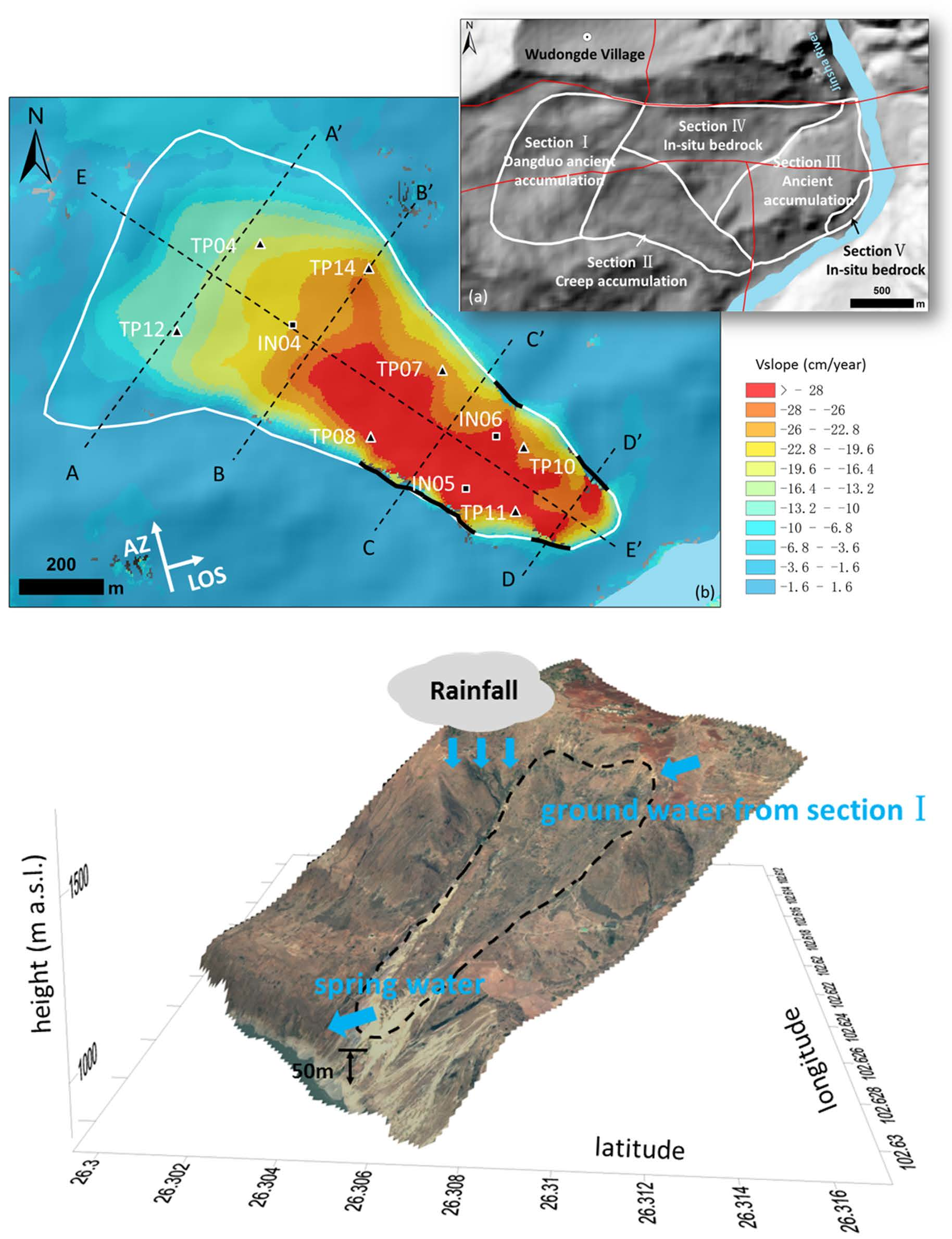
Wudongde Hydropower Station, located in the lower reaches of the Jinsha River in the southwest of China (Figure 1), is one of the key components of the west-east electricity transmission project, which can be used not only for the power generation but also for flood control and sediment flushing [35]. The south bank of the Wudongde reservoir area belongs to Luquan County, Yunnan province, while the north bank belongs to Huidong County, Sichuan province [36]. The reservoir area is located on the southeast border of the Qinghai Tibet Plateau, which is the transition zone between the southwest Sichuan mountain area and the Yunnan-Guizhou Plateau. The study area belongs to the Zhongshan landform, which is affected by tectonic activity and river erosion [37]; therefore, geological disasters occurred frequently in this area [36]. The geomorphology of the study area is much more complex; the lowest area is the valley of Jinsha River, and the depth of the valley generally ranges from 800 to 2000 m, while the altitude of the mountain peak on both sides of the valley ranges from 2500 to 2800 m.
The northwest, southwest and southeast sides of the study area are adjacent to the Songpan-Ganzi Fold System, the Sanjiang Fold System and the Southern China Fold System, respectively [38]. The research area has been influenced by the strong activities of the Western Geosyncline in history, and the folds and faults are well developed. The Bedrock of lower Sinian system of the Neoproterozoic to Mesozoic Upper Cretaceous System and the Quaternary deposits in the Cenozoic are distributed in the study area, and the Quaternary deposits are mainly distributed in the valleys and gentle terrain areas [36,37,38].
The climate of the study area belongs to the subtropical monsoon climate. From the bottom of the valley to the top of the mountain, the climate zones present as Pingba dry and hot valley, hilly and low mountain warm zone, Zhongshan warm area and mountain warm area, etc. [36]. The vegetation includes savannah, pine forest and broadleaf forest. However, the ecological environment has been severely damaged due to deforestation. Most of the area is bare wasteland under the altitude of 2000 m, which is one of the key environmental factors affecting the occurrence of debris flow [36]. Two seasons, namely, dry and rainy seasons, are common in this area; heavy rain and rainstorm weather occurs mainly in the rainy season from May to September, especially from June to August, and extreme rainstorms often result in mudslides, landslides and other disasters [37].
3. Data and Methods
3.1. Data
Twenty L-band archived ALOS/PALSAR images spanning the period from January 2007 to March 2011 with ascending track are included in this study. The interferograms from L-band SAR data have higher coherence than those from the C-band and X- band for the vegetated terrain [39].
To keep the same pixel size between fine-beam double polarization (FBD) and single polarization (FBS) ALOS/PALSAR data, the former is firstly oversampled twice in the range direction. Secondly, to try to detect moderate to small-scale landslides and to map landslides with large deformation, two multilook numbers (One-pixel size is about 7.5 × 7.5 m) are set to generate SAR interferograms [40]. One arc-second shuttle radar topography mission (SRTM) DEM with a pixel size of 30 m is adopted to remove the topographic phase and for the final results analysis.
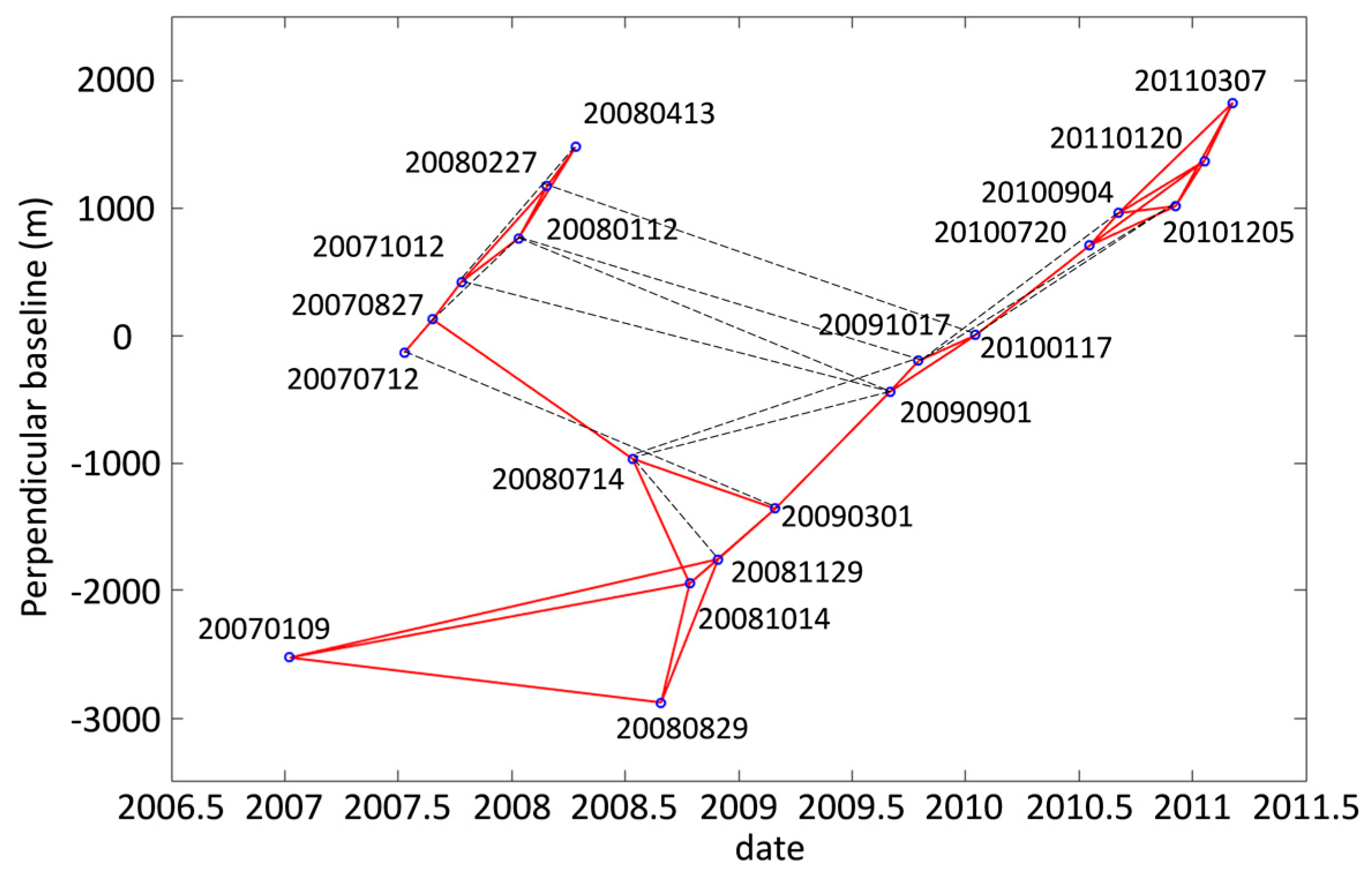
The temporal baseline and the perpendicular baseline thresholds are set to 720 days and 1250 m, respectively. Because the long perpendicular baseline took place in the middle of 2008 for ALOS-1 SAR data, multiple master SAR interferometric pairs are generated. Then, interferograms with heavy atmospheric artefacts and unwrapping errors are visually checked and removed [41,42]. Finally, 31 interferograms are retained as shown in Figure 2, where dashed lines indicate removed interferograms.
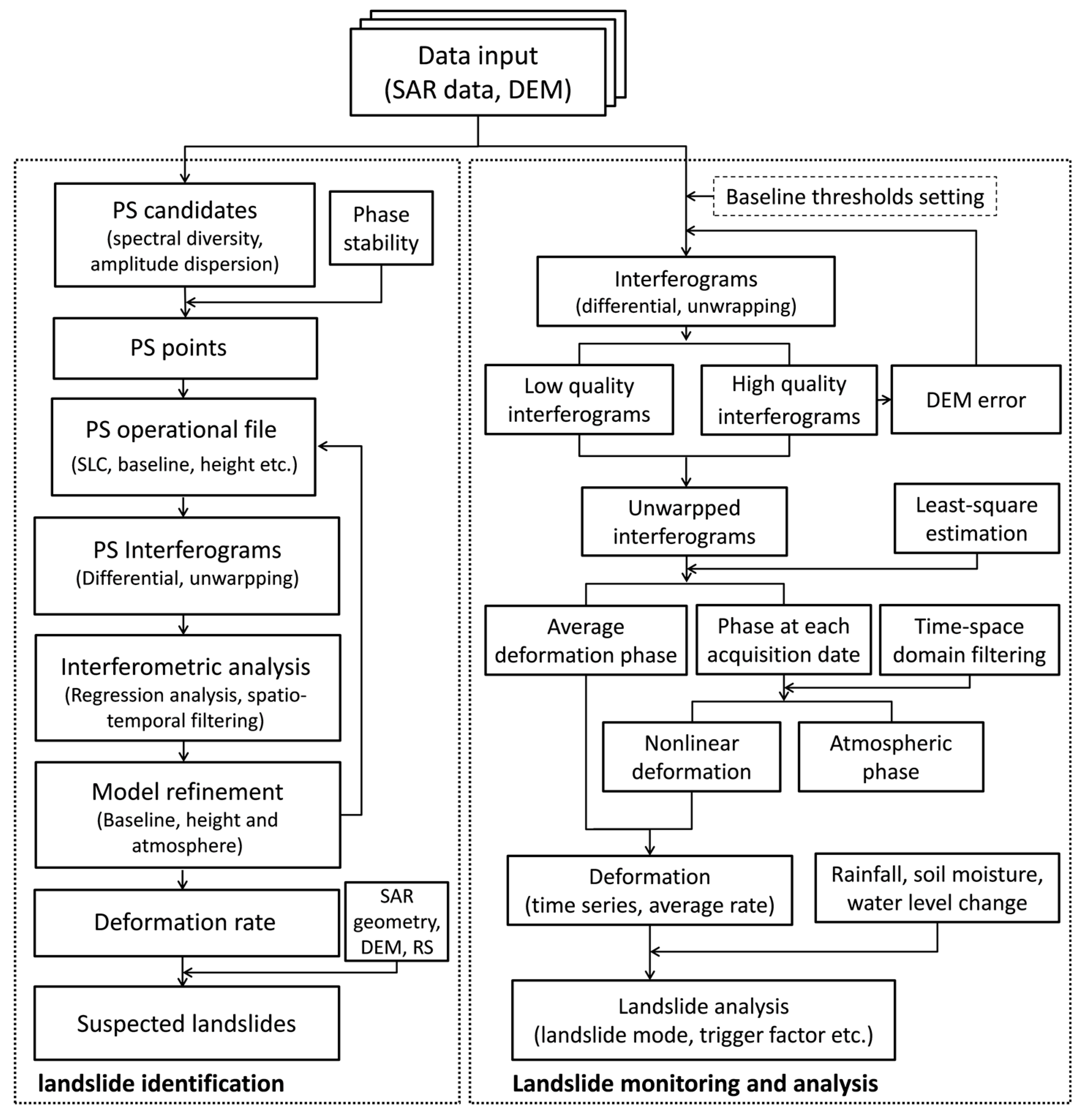
3.2. Flowchart of Landslide Identification and Monitoring
For an unknown region, landslides are firstly identified based on an InSAR-derived deformation map. Then, for a specific landslide, time series deformation will be monitored to obtain a deep understanding of the landslide activities. The flowchart of landslide identification and time series deformation monitoring with InSAR techniques is shown in Figure 3.
3.2.1. Persistent Scatterer Selection
As most landslides occurred in the mountainous regions, the prerequisite for landslide detection is to determine the target points with high quality and a certain density. In this test, three strategies are used to determine Persistent Scatterer (PS) points, namely, spectral diversity [30], amplitude dispersion index and the phase stability [23,43]. Firstly, two sets of PS candidates with low spectral diversity and low amplitude dispersion index are acquired and merged. In addition, PS candidates with low phase stability will be eliminated through two-dimensional regression analysis. Thus, high-quality PS points will be retained.
3.2.2. Landslide Identification
Firstly, IPTA SAR data processing is used to acquire the deformation map [30]. Once the PS points are determined, the wrapped differential phase of PS points on the multi-temporal data stack is calculated with the aid of SRTM DEM, which is interpolated to the slant range radar image coordinate. The linear deformation rate map is generated by the IPTA method. Then, landslides are identified based on the deformation patterns, which can be plotted onto DEM and/or optical remote sensing images. The DEM is mainly used to calculate the slope of the terrain. The areas with a slope angle less than 10 degrees are not considered as landslides in this case. Optical satellite imagery (e.g., Google earth images) is used to determine the landslide boundary. During the specific InSAR monitoring period, obvious deformation may only occur in some parts of the landslide region, which can hardly outline the whole landslide; even some groove and crack or the discontinuity of a stratum can be seen on the spot and can be delineated from the optical satellite imagery [44,45]. In this test, Google earth images are used to roughly depict the extent of the active landslides, which are guided by the InSAR deformation patterns. The main processing steps are summarized as follows:
Step 1. Phase unwrapping. The Minimum Cost Flow (MCF) algorithm based on the Delaunay triangulation network is used for phase unwrapping, i.e., the Delaunay triangulation network is generated based on sparse coherent points [46]. Only unwrapped interferograms can be used to refine the spatial baseline and separate the atmospheric phase.
Step 2. Baseline refinement. In this step, an initial estimation of the linear deformation rate and residual phase is acquired through 2-dimensional (2D) linear regression under the IPTA framework. Then, the terrain phase is added back to the unwrapped differential interferograms, followed by the least square estimation of baseline parameters upon GCPs (Ground control point), from which both the unwrapped phase and corresponding elevation are extracted [47].
Step 3. Atmospheric phase delay (APD) and DEM error estimation. After the baseline refinement, differential interferogram, phase unwrapping, and 2D regression analysis is conducted again. The updated linear deformation rate and DEM error are acquired. The APD can be derived from the residual phase using spatial and temporal filtering [29]. Then, the interferograms are updated by the correction of APD and DEM error.
Step 4. Deformation calculation of PS points. In this step, the linear deformation rate of PS points is calculated by 2D regression analysis of the updated interferograms.
Step 5. Suspected landslides mapping. According to the deformation patterns and combined with SAR geometry, e.g., look angle, DEM and optical remote sensing images, locations and extents of the suspected landslides can be mapped.
3.3. Landslide Time Series Deformation Monitoring
Due to the small volume of SAR data, the SBAS-InSAR method is applied to retrieve the continuous deformation field in the spatial domain and time series deformation in the time domain for the specific landslide [20]. The differential interferograms are divided into high-quality sets and low-quality sets. The former are used to estimate the DEM error. After the DEM error correction, all interferograms are used to estimate the average deformation phase and the phase for each SAR acquisition date. As the atmospheric phases are spatially correlated and temporally random, the APD can be separated through low-pass filtering and high-pass filtering in the space and time domains, respectively [29]. The remainder is the nonlinear deformation phase, which can be added back to the average deformation phase, and the cumulative deformation can be trivially acquired for each SAR acquisition date. In most cases, the earliest SAR acquisition date is set as the reference date. The abovementioned procedure is conducted in single datasets with least square criteria. Once there is more than one dataset, the deformation between adjacent datasets has to be constrained by some smooth assumption or given by the external measurements.
4. Results and Analysis
4.1. Landslides Identification Results
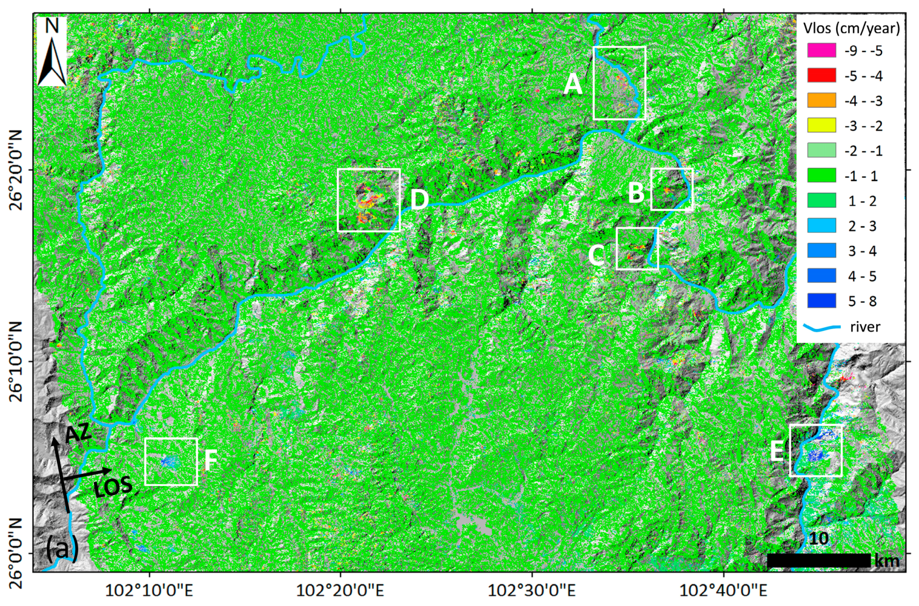
The InSAR products including intensity maps and coherence maps and external DEM could be used to detect and map landslides that occur suddenly with a certain extent [48], while the deformation map is beneficial to identify the potential, slow, and long-term deformed landslides. In this experiment, twenty-two landslides covering an area of approximate 2500 km2 are identified from the InSAR derived deformation map, as shown in Figure 4. As the deformation is illuminated in the line-of-sight (LOS) direction, please note that the red in Figure 4a and Figure 5 indicates the movement close to the sensor, while the blue is away from the sensor. Figure 4b shows the suspected landslide locations. It is obvious that most of the suspected landslides are developed on both sides of the valley, which can be explained by the special geomorphology. The valley of Jinsha River, deep and narrow with a 500~2000 m cutting depth, affected by strong water erosion, forms the landslide-prone region.
As landslides are often constrained by topography, optical images can be used as the background for landslide boundary delineation and the deformation illustration, on which the whole landslide including active or inactive regions can be seen with discontinuous landforms [44,49]. Landslides in 6 regions in Figure 4a are enlarged and superimposed on perspective Google earth images, shown in Figure 5. It can be found that the obvious features of landslide and debris flow gully, such as a groove and a crack can be seen clearly from the Google earth images.
In order to further confirm the identified suspected landslides, published literature was reviewed [35,36,37,50,51,52], and 9 of the 22 landslides have already been documented as follows: No. 10 in Figure 4 is the Yangpingzi unstable rock mass, No. 11 is the Huashan landslide, No. 13 is the Qianchang unstable rock mass, No. 14 is the Dacun-Fujiapingzi landslide, No. 15 is the Dapingdi landside, No. 16 is the Jinpingzi landslide, both No. 17 and 18 belong to the Shuanglongtan debris flow, and No. 20 is the Pufu landslide. It should be noted that the abovementioned landslides are recorded due to their prior occurrence; other suspected landslides that have not been found in the relevant literature might be potential landslides, which means much more attention should be given to prevent or reduce the hazards.
4.2. Landslide Deformation Monitoring Analysis
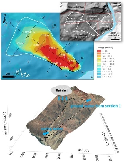
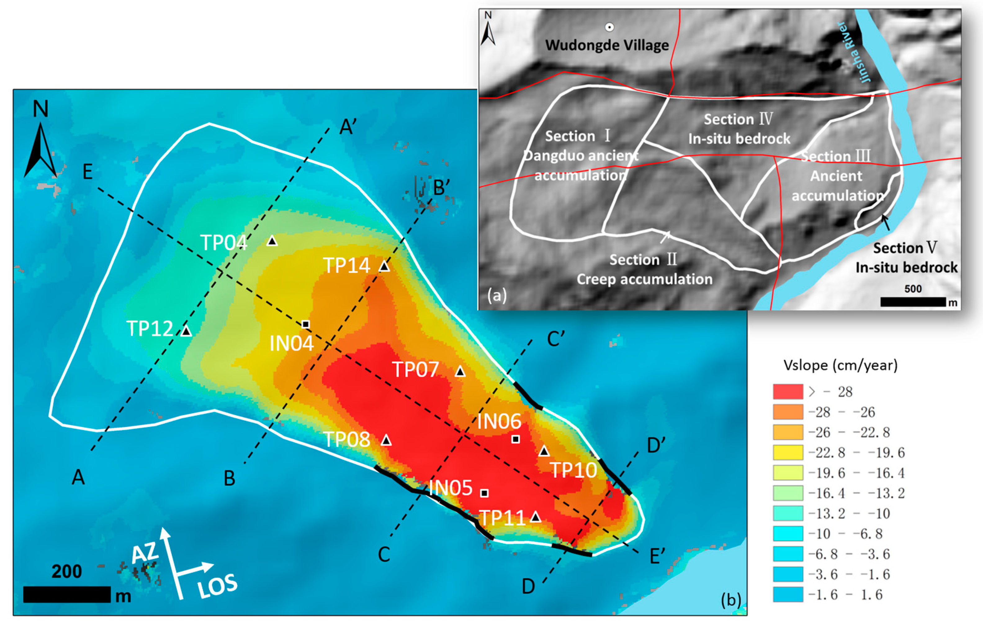
Jinpingzi landslide, labeled as No. 16 in Figure 4b, which is focused on to show spatial and time series deformation features, is settled on the right bank of Jinsha River in the lower reach of the Wudongde Hydropower Station. The landslide is divided into 5 sections according to its topography, geomorphology and geological features shown in Figure 6a as follows, Dangduo ancient accumulation (Section I), creep accumulation (Section II), Jinpingzi ancient accumulation (Section III), in-situ bedrock (Section IV) and bedrock outcrops (Section V) in the leading edge of the Jinpingzi ancient accumulation [51]. The elevation of the leading edge is about 820 m, and the elevation of the trailing edge ranges from 1900 m to 2200 m. The total volume of the landslide is about 620 million cubic meters [51]. Section II is the most unstable block among these sections, which has been monitored with in-situ equipment for a long time [37,51]. The slope of Section II is from 18 to 36 degrees (the average slope angle is about 23 degree), and the total volume of this section reaches 27 million cubic meters. Once this section slumps, a tremendous disaster will occur.
4.2.1. Deformation Results
Archived SAR data spanning the period from January 2008 to March 2011 are considered to obtain the time-series deformation over Jinpingzi landslide through the SBAS-InSAR technique. Fifteen pairs of high quality interferograms are used for time series deformation monitoring after removal of low quality interferograms, which belongs to three subsets as shown in Table 1. Then, the LS norm is used to obtain the time-series deformation for each subset, and the average deformation rate is acquired by the stacking interferogram method [53].
4.2.2. Spatial Deformation Characteristics
It can be seen in Figure 6b that the surface deformation in the leading section of the landslide was larger than that in the trailing section. Accordingly, this landslide may belong to a pull-type landslide. The maximum downslope deformation rate occurred at the southernmost corner of the leading section, which reached 39 cm/year.
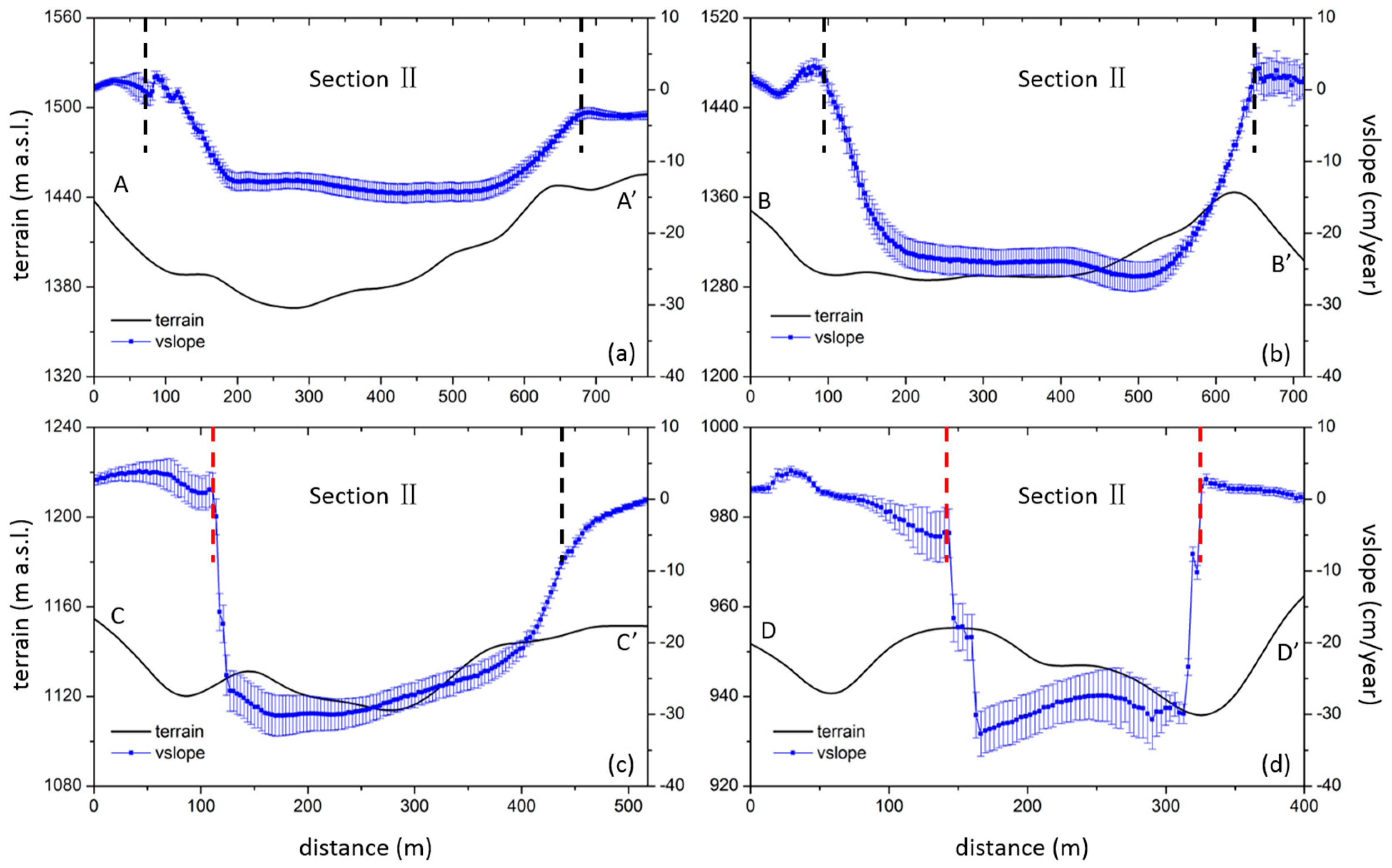
The deformation rate and the terrain of the landslide are extracted along four transverse lines, as shown in Figure 7. It can be seen that the width of landslide gradually decreases from the trailing section to the leading section. The deformed region is controlled by two boundaries, where several slide-bounding strike-slip fissures can be detected as shown in Figure 6a. In Figure 6 and Figure 7, abrupt deformation changes can be obviously seen across some parts of boundaries, which is similar to the strike-slip fault deformation [54]. Especially in Figure 7c,d, the deformation rate suddenly drops from 30 cm/y to 0 cm/y within 20 m crossing the boundaries, and the obvious discontinuity of these boundaries can be seen in the Google image. This kind of boundary, i.e., similar to strike-slip faults, has been found in some other landslides detected by field investigation or geophysical prospecting method [55,56,57,58]. The slidequake generation is generally correlated with these boundaries, which play a significant role in the landslide movement [58]. In this paper, this kind of boundary can be clearly mapped from the InSAR deformation map (as shown in Figure 6).
On the other hand, it can also be seen that the transverse topography gradually transformed from concave terrain to convex terrain from the trailing section to the leading section of the landslide (as shown in Figure 6a and Figure 7), indicating that the materials were deposited in the leading section from the trailing section during the long-term landslide creeping.
In addition, it can be found that the deformation at the leading edge of Section II changed very sharply; quantitatively speaking, the maximum cumulative deformation changed quickly from −45 to 0 cm within 100 m, which indicates that the exposed bedrock in front of Section II prevents the landslide movement. Secondly, due to the wedged shaped landslide with a narrow leading section and wide trailing section, the boundaries on both sides of the landslide have anti-slip force relative to the landslide. Furthermore, the fault in front of the landslide plays a key role in landslide deformation.
4.2.3. Comparison of Interferometric Synthetic Aperture Radar Deformation with Georobot Measurements
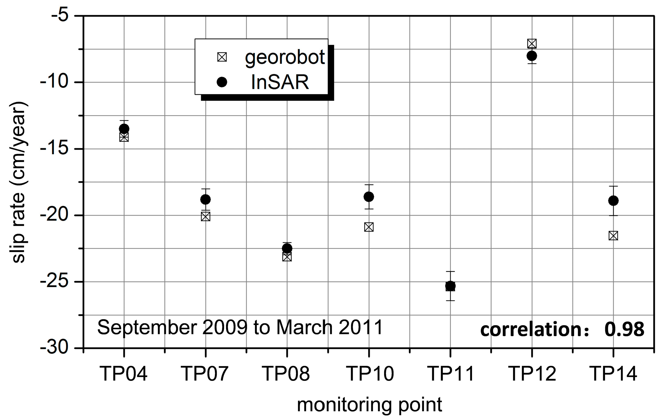
Section II of the landslide has been continuously monitored with georobot since January 2005 [59,60]. The total displacement of each georobot monitoring point is compared with the InSAR deformation in the downslope direction. Firstly, the slip rate results over seven georobot benchmarks are compared with InSAR measurements from Sep. 2009 to Mar. 2011 (the third monitoring subsets are presented in Table 1, and the time series deformation of the third subsets is shown in Figure 8.
As shown in Figure 9, the error bar of the InSAR results represent the uncertainty with RMS (root mean square error) of the slip rate results within the region of the 50 m × 50 m area around the georobot monitoring point. We find that the largest difference is located at TP14, which has reached 2.6 cm/y. Except for TP10 and TP14, the difference of the other five points is less than 1.3 cm/y. To compare InSAR measurements with georobot measurements, all InSAR deformation in LOS is transferred to the landslide downslope direction using uniform landslide geometry. However, the local landslide movement directions are slightly different in different parts; therefore, discrepancies for some points can be found.
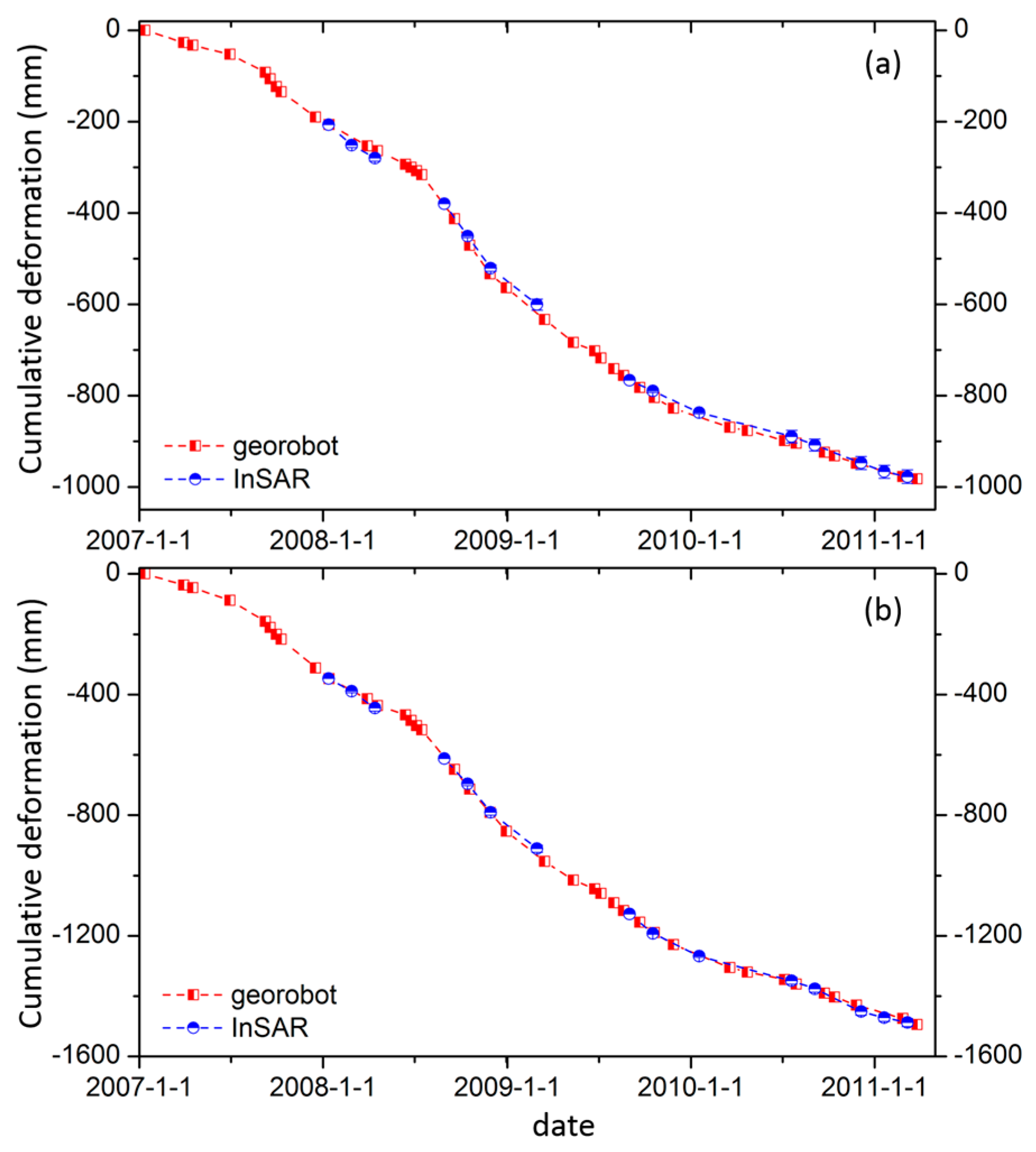
Then, time series InSAR and georobot monitoring results from 2007 to 2011 are compared at two benchmarks of points TP04 and TP08. Since the datum of the deformation sequence acquired by the georobot is different from the one acquired by InSAR, the initial offsets of each InSAR subset are considered with respect to the time series deformation measured by georobot. It is clear that the time series deformations acquired by InSAR are strongly consistent with georobot measurements. Considering the locations of points TP04 and TP08, the surface deformation at the lower terrain (TP04) was larger than that at the higher terrain (TP08), while the two points have similar deformation trends from 2007 to 2011 (as shown in Figure 10).
5. Discussion
5.1. Landslide Type
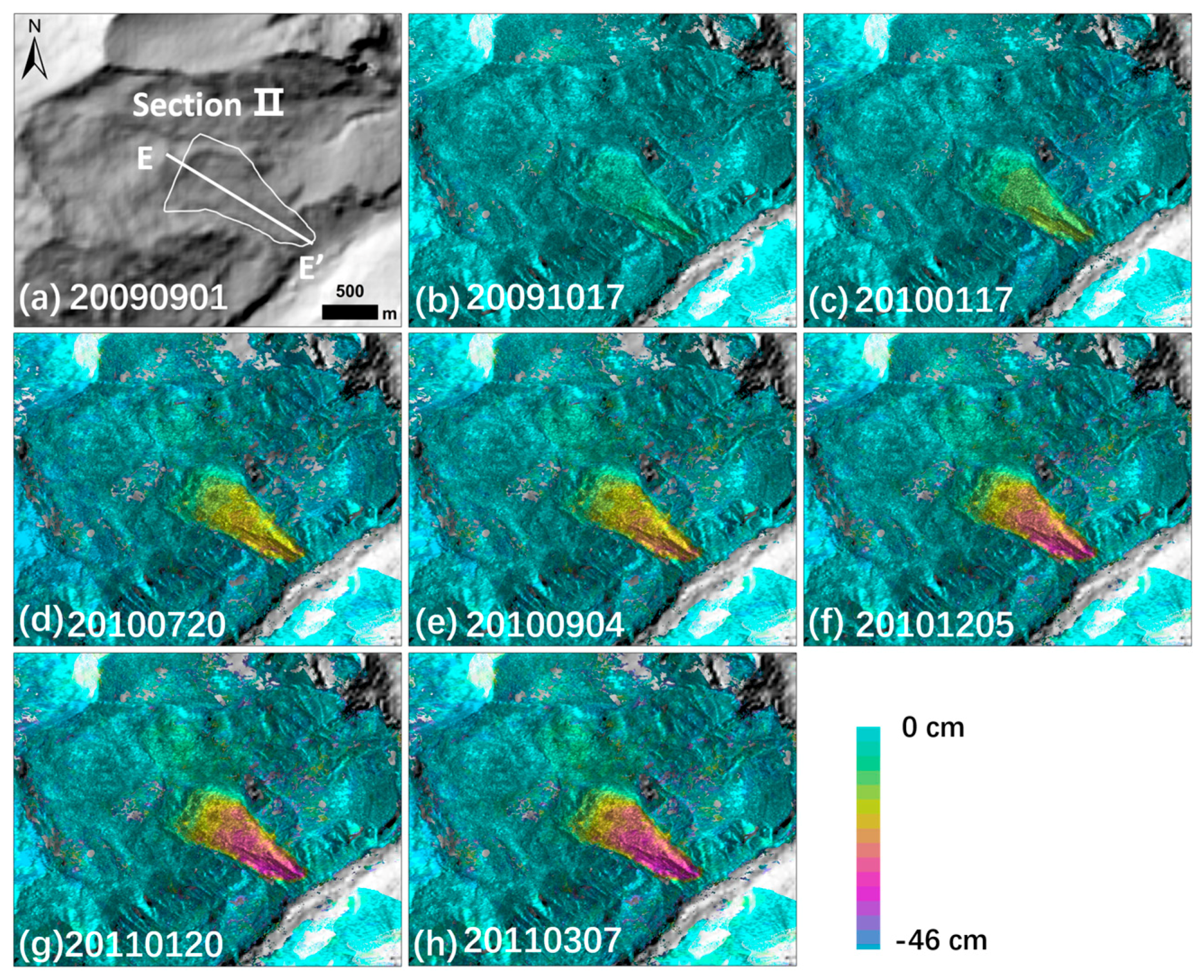
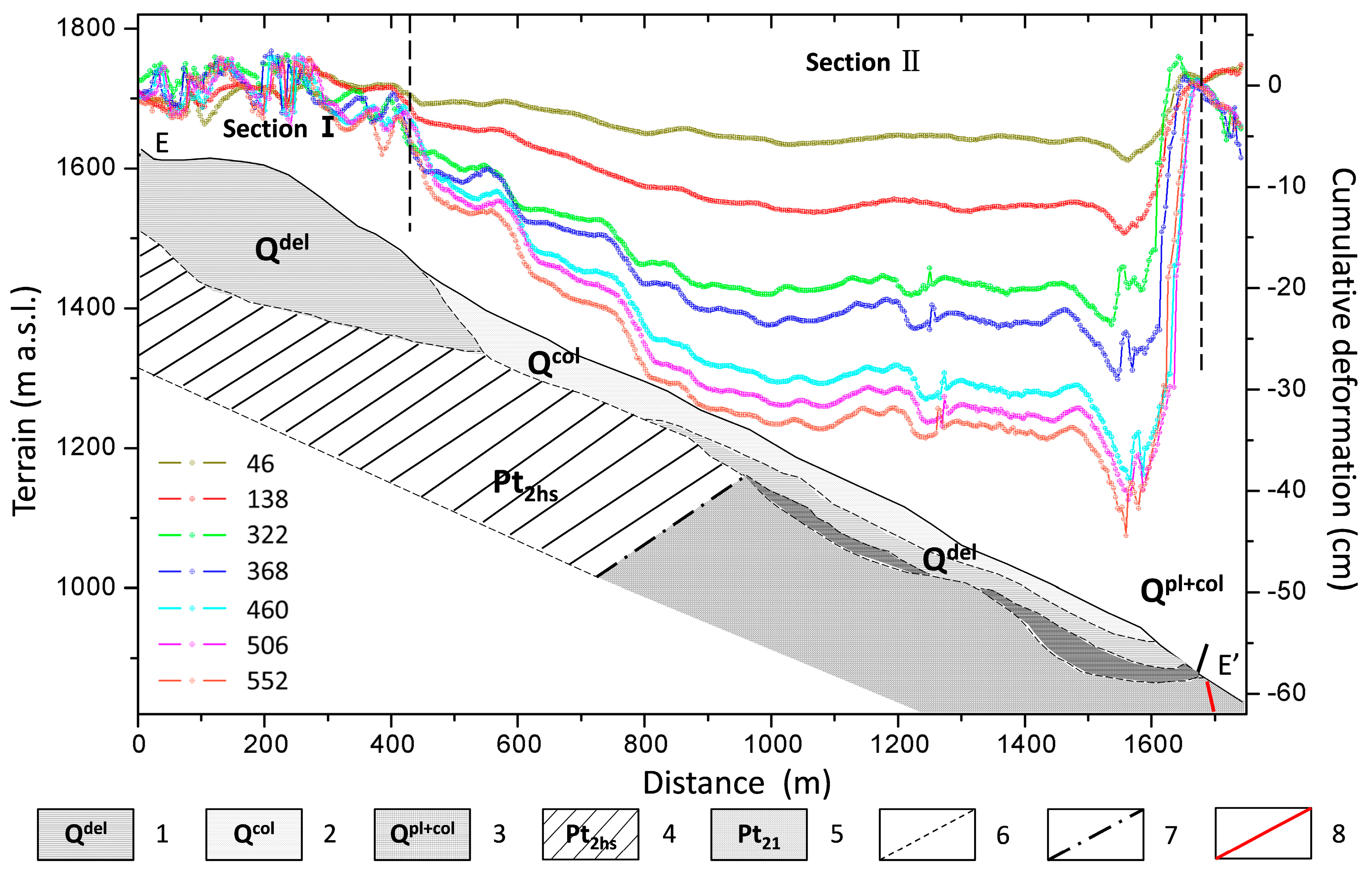
For further analysis of the spatiotemporal deformation characteristics of the landslide, the cumulative time-series deformation along profile EE’ is abstracted and superimposed on the geological cross-section map, shown in Figure 11. As the interferograms are divided into three subsets, the third subset from 20090901 to 20110307 is selected for the time series deformation analysis. The earliest SAR acquisition date of the third subset is taken as the reference date, labeled as 20090901 in Table 1. The numbers in Figure 11 indicate the accumulated days from the reference date.
The thickness of the landslide can be deduced from borehole, adit and sonic wave data from 45 to 100 m [51,59]. The thickness in the front of section ranges from 90 to 130 m; in the middle section, ranges from 80 to 90 m; and in the rear section, ranges from 45 to 60 m. According to its material composition and geological structure, the landslide can be divided into 3 layers from bottom to top, that is, (i) Gravel with a small amount of silt (Qpl+col), which distributes in the front and middle ancient gullies of the sliding body, with a thickness ranging from 30 to 64 m; (ii) Clastic soil of the phyllite (Qdel), with a thickness ranging from 16 to 45 m; (iii) Dolomite gravel with a small amount of silt, which is widely distributed in the upper part of the slide mass, with a thickness ranging from 20 to 61 m. Geological reconnaissance showed the landslide belongs to the pull-type landslide, and the sliding surface is located in the lower part of the clastic soil of the phyllite formation (Qdel), the clastic soil of the phyllite and the gravel with a small amount of silt retrogressive creeping along the sliding surface [59]. As shown in Figure 6 and Figure 8, the deformation occurred mainly in the Section II area and gradually increased with decreasing landslide height, which further confirms that the landslide belongs to the pull-type landslide.
Three inclinometers were placed in Section II of Jinpingzi landslide, so the inner displacement of the landslide was obtained [51]. However, the monitoring period was different between InSAR and inclinometers, so the closest InSAR monitoring period to the inclinometer monitoring period was chosen for rough comparison (as shown in Table 2). Inner displacement shows that the depth of this landslide is mainly at around 55 m beneath the surface, which can be defined as the sliding surface [51]. It can also be seen that the inner deformation was larger than that at the surface, and the deformation in the leading section was larger than that at the tailing section for both the surface and inner point. Accordingly, it can be deduced that this landslide belongs to a pull-type landslide.
5.2. Environmental Factor Analysis
The activity of landslide is often affected by several environmental factors such as rainfall, soil moisture and river water level changes [61,62,63,64,65,66]. The correlation among precipitation, soil moisture, water level changes of the Jinsha River and the Jinpingzi landslide deformation rate is analyzed.
Firstly, 20 ALOS/PALSAR data are used to measure water level changes. As shown in Figure 11, the different SAR intensity images can reflect the water level changes, and it can be found that the water level in the rainy season is obviously higher than that in the dry season. To this end, all SAR intensity images are used to measure the water level changes according to the waterline and local terrain in different dates. Since the water body in SAR intensity shows low back scatter characteristics, the water level can be easily detected, as shown in red in Figure 12.
Secondly, the backscattering coefficient of the SAR intensity image is used to inverse the soil moisture changes, as the increase in soil moisture results in an increase in radar backscattering [67]. In sparsely vegetated areas, the backscattering coefficient can be expressed as
where σ0 is the backscattering coefficient, h(θ) depends on the incidence angle θ, g is the surface roughness function, s is the surface rms, l is the surface correlation length, Γ(0) is the Fresnel reflectivity, which can be expressed as
where Mv is the soil volumetric moisture. Therefore, in the case of the same incident angles, the backscattering coefficient of SAR intensity images mainly depends on the surface roughness and soil moisture. As changes in surface roughness would modify the relative positions of the scatter within each pixel, which will affect both the intensity and the phase information of the backscattering signal, coherence can be used as a reflection of surface roughness change [68]. We calculated the average SAR intensity of the area with a coherence value more than 0.65 for each selected interferograms (as shown in Figure 2) to inverse the soil moisture change. Then, the landslide deformation, rainfall, soil moisture and water level changes are analyzed.
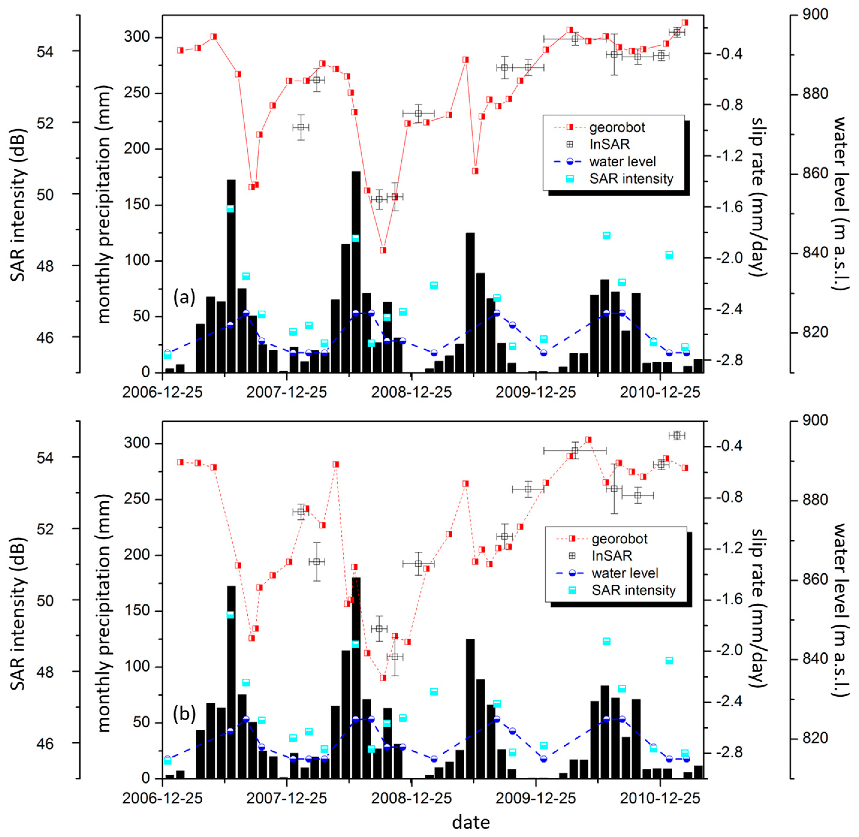
Figure 13 shows the correlation among Jinsha River water level changes, monthly precipitation and daily deformation rate acquired by InSAR and georobot for the monitoring points TP08 and TP04, where error bars of the InSAR monitoring in the vertical component represent the uncertainty of the InSAR slip rate, and in the horizontal direction represent the time interval between two adjacent SAR acquisition dates. Some conclusions can be drawn as follows:
- (i)
- The fluctuation of the water level in the Jinsha River is almost similar in each year during the monitoring period. The water levels of the reservoir area in July and August 2010 are the same as those in July and August 2007, but the landslide deformation in 2007 is much larger than that in 2010, which indicates that the fluctuation of the Jinshajiang river water is not the main influential factor of the landslide movement.
- (ii)
- Qualitatively, the SAR intensity in the rainy season is obviously higher than that in the dry season, which means that the SAR intensity can reflect the surface soil moisture to a certain extent. Accordingly, certain correlation between surface soil moisture and the total precipitation can be found, but there is a weak correlation between surface soil moisture and the landslide deformation.
- (iii)
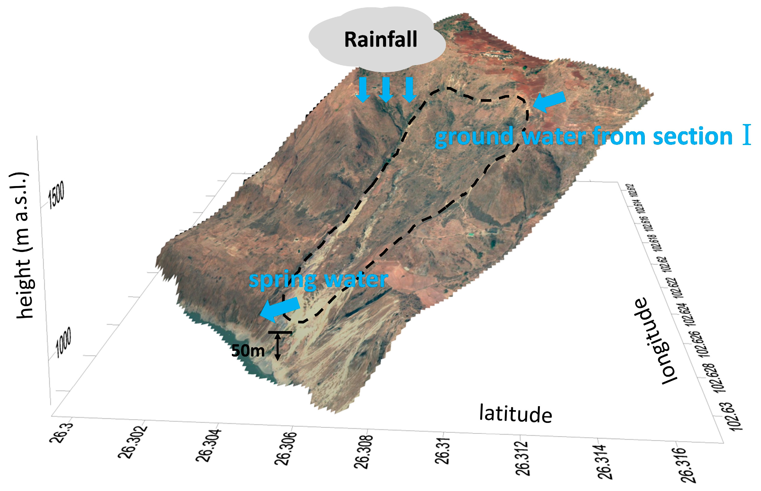
- During the rainy season, the monitoring result obtained from both georobot and InSAR is more sensitive to heavy precipitation events than to the total precipitation volume. As shown in Figure 14, the groundwater recharge of Section II is mainly from rainfall and the groundwater from Section I [51]. The aquifer of Section II is located at the lower part of the third layer (Qcol) and the upper part of the second layer (Qdel), so the underground water is blocked by slip band soil which is located under the aquifer, and is discharged as a spring at the leading edge of Section II [59]. As measured at the spring, the total discharge of groundwater is about 230 m3/d, and normally, the amount of the supplement and the discharge of the groundwater in this section are in a state of balance [59]. We suggest that when heavy rainfall occurs, the total amount of groundwater recharge is larger than the groundwater discharge, resulting in more water entering the sliding surface, which on the one hand decreases the shear strength of the landslide [65] and on the other hand increases the weight of the landslide. As a consequence, the landslide velocity will increase.
- (iv)
- The maximum deformation of the landslide was highly consistent with the peak precipitation with a time lag of about 1 to 2 months. Quantitatively, the correlations of deformation and precipitation at the two monitoring points are only 0.3 and 0.4, respectively. If a one-month time lag is considered, the correlations increase to 0.56 and 0.55, respectively. However, due to the long ALOS/PALSAR satellite revisit time, it is difficult to identify the fine lag time between heavy precipitation and landslide onset. This finding can be verified with periodic in-situ three dimensional measurements [60].
6. Conclusions
The processes of landslide identification and monitoring by InSAR methods are presented, among which four key steps are outlined. The annual deformation rate map in line-of-sight direction generated with the IPTA InSAR technique is used for landslide identification, and 22 suspected landslides located on two sides of Jinsha River valley are identified over an area more than 2500 km2; it can be deduced that water erosion is the landslide mechanism. The SBAS InSAR technique is applied to achieve time-series deformation maps over Section II of Jinpingzi landslide. This landslide deformation is controlled by the faults, geological formation and geomorphological structure. Considerable evidence, including surface and inner deformation features, indicates that this landslide belongs to a pull-type landslide. High InSAR deformation monitoring accuracy is obtained by the InSAR method in the comparison with in-situ georobot measurements, and the maximum downslope deformation rate reached 39 cm/y. The deformation of the landslide was very sensitive to heavy precipitation, and a 1- to 2-month time lag between the peak of the precipitation and the maximum deformation rate has been revealed. As a next step, and in order to better understand the movement of the landslide and its potential for further movement (a) the location of the slip surface must be identified, (b) the soil type along the slip surface will be detected and (c) the soil strength along the slip surface will be measured and/or estimated by back analyses using the recently proposed approach proposed by Stamatopoulos and Di and Di et al [69,70].
Our research provides a systematic procedure with the InSAR technique for landslide inventory mapping, deformation monitoring, trigger factor verification and landslide mode deductions, which will be beneficial to early warning system development for remote mountainous landslides under abnormal rainfall conditions.
Author Contributions
C.Z. and Y.K. performed the experiments and produced the results. C.Z. drafted the manuscript. Q.Z., Z.L., and B.L. contributed to the discussion of the results. B.L. helped to collect and analyze the in-situ data. All authors conceived of the study and reviewed and approved the manuscript.
Funding
This research was funded by the Natural Science Foundation of China [41731066, 41628401, 41504005], the Fundamental Research Foundation of the Central Universities [300102268704], the Ministry of Land & Resources (China) projects [DD20160268] and the 111 project [B18046.
Acknowledgments
ALOS/PALSAR data are provided by JAXA, Japan, and the one-arc-second SRTM DEM was freely downloaded from the website http://e4ftl01.cr.usgs.gov/MODV6_Dal_D/SRTM/SRTMGL1.003/2000.02.11/.
Conflicts of Interest
The authors declare no conflicts of interest.
References
- Liu, P.; Li, Z.; Hoey, T.; Kincal, C.; Zhang, J.; Zeng, Q.; Muller, J. Using advanced InSAR time series techniques to monitor landslide movements in Badong of the Three Gorges region, China. Int. J. Appl. Earth Obs. Geoinf. 2013, 21, 253–264. [Google Scholar] [CrossRef]
- Huang, B.L.; Yin, Y.P.; Liu, G.N.; Wang, S.C.; Chen, X.T.; Huo, Z.T. Analysis of waves generated by Gongjiafang landslide in Wu Gorge, three Gorges reservoir, on November 23, 2008. Landslides 2012, 9, 395–405. [Google Scholar] [CrossRef]
- Michoud, C.; Baumann, V.; Lauknes, T.R.; Penna, I.; Derron, M.H.; Jaboyedoff, M. Large slope deformations detection and monitoring along shores of the potrerillos dam reservoir, Argentina, based on a small-baseline InSAR approach. Landslides 2016, 13, 451–465. [Google Scholar] [CrossRef]
- Fell, R.; Corominas, J.; Bonnard, C.; Cascini, L.; Leroi, E.; Savage, W.Z. Guidelines for landslide susceptibility, hazard and risk zoning for land use planning. Eng. Geol. 2008, 102, 85–98. [Google Scholar] [CrossRef] [Green Version]
- Guzzetti, F.; Mondini, A.C.; Cardinali, M.; Fiorucci, F.; Santangelo, M.; Chang, K.T. Landslide inventory maps: New tools for an old problem. Earth-Sci. Rev. 2012, 112, 42–66. [Google Scholar] [CrossRef]
- Crosta, G.B.; Frattini, P.; Agliardi, F. Deep seated gravitational slope deformations in the European Alps. Tectonophysics 2013, 605, 13–33. [Google Scholar] [CrossRef]
- Ding, X.; Montgomery, S.B.; Tsakiri, M.; Swindells, C.F.; Jewell, R.J. Integrated Monitoring Systems for Open Pit Wall Deformation; Meriwa Report No. 186; Australian Centre for Geomechanics: Perth, Australia, 1998. [Google Scholar]
- Thompson, P.W.; Cierlitza, S. Identification of a slope failure over a year before final collapse using multiple monitoring methods. In Geotechnical Instrumentation and Monitoring in Open Pit and Underground Mining; Szwedzicki, T., Ed.; AA Balkema: Rotterdam, The Netherlands, 1993. [Google Scholar]
- Massonnet, D.; Feigl, K.L. Radar interferometry and its application to changes in the Earth’s surface. Rev. Geophys. 1998, 36, 441–500. [Google Scholar] [CrossRef]
- Bulmer, M.H.; Petley, D.N.; Murphy, W.; Mantovani, F. Detecting slope deformation using two-pass differential interferometry: Implications for landslide studies on Earth and other planetary bodies. J. Geophys. Res. Planets 2006, 111. [Google Scholar] [CrossRef] [Green Version]
- Cascini, L.; Fornaro, G.; Peduto, D. Advanced low- and full-resolution DInSAR map generation for slow-moving landslide analysis at different scales. Eng. Geol. 2010, 112, 29–42. [Google Scholar] [CrossRef]
- Farina, P.; Colombo, D.; Fumagalli, A.; Marks, F.; Moretti, S. Permanent scatterers for landslide investigations: Outcomes from the ERS-SLAM project. Eng. Geol. 2006, 88, 200–217. [Google Scholar] [CrossRef]
- Pierson, T.; Lu, Z. InSAR detection of renewed movement of a large ancient landslide in the Columbia River Gorge, Washington. In Proceedings of the Geological Society of America 2009 Annual Meeting, Portland, OR, USA, 18–21 October 2009. [Google Scholar]
- Hu, X.; Wang, T.; Pierson, T.C.; Lu, Z.; Kim, J.; Cecere, T.H. Detecting seasonal landslide movement within the cascade landslide complex (Washington) using time-series SAR imagery. Remote Sens. Environ. 2016, 187, 49–61. [Google Scholar] [CrossRef]
- Intrieri, E.; Raspini, F.; Fumagalli, A.; Lu, P.; Conte, S.D.; Farina, P. The Maoxian landslide as seen from space: Detecting precursors of failure with sentinel-1 data. Landslides 2017, 15, 123–133. [Google Scholar] [CrossRef]
- Kang, Y.; Zhao, C.Y.; Zhang, Q.; Lu, Z.; Li, B. Application of InSAR techniques to an analysis of the Guanling landslide. Remote Sens. 2017, 9, 1046. [Google Scholar] [CrossRef]
- Calabro, M.D.; Schmidt, D.A.; Roering, J.J. An examination of seasonal deformation at the Portuguese Bend landslide, southern California, using radar interferometry. J. Geophys. Res. Earth Surface 2010, 115. [Google Scholar] [CrossRef] [Green Version]
- Catani, F.; Farina, P.; Moretti, S.; Nico, G.; Strozzi, T. On the application of SAR interferometry to geomorphological studies: Estimation of landform attributes and mass movements. Geomorphology 2005, 66, 119–131. [Google Scholar] [CrossRef]
- Strozzi, T.; Farina, P.; Corsini, A.; Ambrosi, C.; Thüring, M.; Zilger, J.; Wiesmann, A.; Wegmüller, U.; Wener, C. Survey and monitoring of landslide displacements by means of L-band satellite SAR interferometry. Landslides 2005, 2, 193–201. [Google Scholar] [CrossRef]
- Berardino, P.; Costantini, G.; Franceschetti, G.; Iodice, L.; Pietranera, L.; Rizzo, V. Use of differential SAR interferometry in monitoring and modeling large slope instability at Matera (Basilicata, Italy). Eng. Geol. 2003, 68, 31–51. [Google Scholar] [CrossRef]
- Zhu, W.; Zhang, Q.; Ding, X.; Zhao, C.; Yang, C.; Qu, F.; Qu, W. Landslide monitoring by combining of CR-InSAR and GPS techniques. Adv. Space Res. 2014, 53, 430–439. [Google Scholar] [CrossRef]
- Xia, Y.; Kaufmann, H.; Guo, X.F. Landslide monitoring in the Three Gorges area using D-INSAR and corner reflectors. Photogramm. Eng. Remote Sens. 2004, 70, 1167–1172. [Google Scholar]
- Hooper, A.; Segall, P.; Zebker, H. Persistent scatterer InSAR for crustal deformation analysis, with application to Volca’nAlcedo, Gala’pagos. J. Geophys. Solid Earth. 2007, 112, B07407. [Google Scholar]
- Hooper, A.; Zebker, H.; Segall, P.; Kampes, B. A new method for measuring deformation on volcanoes and other natural terrains using InSAR persistent scatterers. Geophys. Res. Lett. 2004, 31. [Google Scholar] [CrossRef] [Green Version]
- Ferretti, A.; Fumagalli, A.; Novali, F.; Prati, C.; Rocca, F.; Rucci, A. A new algorithm for processing interferometric data-stacks: SqueeSAR. IEEE Trans. Geosci. Remote Sens. 2011, 49, 3460–3470. [Google Scholar] [CrossRef]
- Leva, D.; Nico, G.; Tarchi, D.; Fortuny, G.J.; Sieber, A.J. Temporal analysis of a landslide by means of a ground-based SAR interferometer. IEEE Trans. Geosci. Remote Sens. 2003, 41, 745–752. [Google Scholar] [CrossRef]
- Zhao, C.Y.; Lu, Z.; Zhang, Q.; Fuente, J.D.L. Large-area landslide detection and monitoring with ALOS/PALSAR imagery data over northern California and southern Oregon, USA. Remote Sens. Environ. 2012, 124, 348–359. [Google Scholar] [CrossRef]
- Samsonov, S.; van der Kooij, M.; Tiampo, K. A simultaneous inversion for deformation rates and topographic errors of DInSAR data utilizing linear least square inversion technique. Comput. Geosci. 2011, 37, 1083–1091. [Google Scholar] [CrossRef]
- Ferretti, A.; Prati, C.; Rocca, F. Permanent scatterers in SAR interferometry. IEEE Trans. Geosci. Remote Sens. 2001, 39, 8–20. [Google Scholar] [CrossRef] [Green Version]
- Werner, C.; Wegmuller, U.; Strozzi, T.; Wiesmann, A. Interferometric point target analysis for deformation mapping. In Proceedings of the IGARSS 2003, Toulouse, France, 21–25 July 2003. [Google Scholar]
- Furuya, M.; Mueller, K.; Wahr, J. Active salt tectonics in the Needles District, Canyonlands (Utah) as detected by interferometric synthetic aperture radar and point target analysis: 1992–2002. J. Geophys. Res. Solid Earth 2007. [Google Scholar] [CrossRef]
- Yan, Y.; Doin, M.P.; Lopez-Quiroz, P.; Tupin, F.; Fruneau, B.; Pinel, V.; Trouvé, E. Mexico city subsidence measured by InSAR time series: Joint analysis using PS and SBAS approaches. IEEE. J-STARS 2012, 5, 1312–1326. [Google Scholar] [CrossRef] [Green Version]
- Schlögel, R.; Doubre, C.; Malet, J.P.; Masson, F. Landslide deformation monitoring with ALOS/PALSAR imagery: A D-InSAR geomorphological interpretation method. Geomorphology 2015, 231, 314–330. [Google Scholar] [CrossRef]
- Zhang, L.; Liao, M.S.; Balz, T.; Shi, X.G.; Jiang, Y.N. Monitoring landslide activities in the three gorges area with multi-frequency satellite SAR data sets. In Modern Technologies for Landslide Monitoring and Prediction; Scaioni, M., Ed.; Springer: Berlin/Heidelberg, Germany, 2015; pp. 181–208. [Google Scholar]
- Wang, L.W. Identification of Landslide Displacement in Alpine Valley Region Based on D-InSAR Data Analysis. Ph.D. Thesis, University of Science and Technology Beijing, Beijing, China, 2014. [Google Scholar]
- Wu, J.M. The Disciplinarian on the Development and Distributing of Geo-disaster & Stability Evaluation of the Bank Slope in Wudongde Reservoir Area of the Jinsha River. Master’s Thesis, Chengdu University of Technology, Chengdu, China, 12 July 2009. [Google Scholar]
- Zhang, W. Research of Evaluation Methods for Rock Mass Structures in the Wudongde Hydropower Reservoir Region. Ph.D. Thesis, Jilin University, Changchun, China, 1 June 2013. [Google Scholar]
- Hu, Q.F. Study on Landslide Hazards Risk of Wudongde Bank. Master’s Thesis, Changjiang River Scientific Research Institute, Wuhan, China, 5 May 2014. [Google Scholar]
- Lu, Z.; Dzurisin, D.; Jung, H.S.; Zhang, J.; Zhang, Y. Radar image and data fusion for natural hazards characterization. Int. J. Image Data Fusion. 2010, 1, 217–242. [Google Scholar] [CrossRef]
- Zhao, C.Y.; Zhang, Q.; Yin, Y.; Lu, Z.; Yang, C.; Zhu, W.; Li, B. Pre-, co-, and post-rockslide analysis with ALOS/PALSAR imagery: A case study of the Jiweishan rockslide, China. Nat. Hazard. Earth Syst. Sci. 2013, 13, 2851–2861. [Google Scholar] [CrossRef]
- Zhao, C.Y.; Zhang, Q.; He, Y.; Peng, J.B.; Yang, C.S.; Kang, Y. Small-scale loess landslide monitoring with small baseline subsets interferometric synthetic aperture radar technique—Case study of Xingyuan landslide, Shaanxi, China. J. Appl. Remote Sens. 2016, 10. [Google Scholar] [CrossRef]
- Motagh, M.; Wetzel, H.U.; Roessner, S.; Kaufmann, H. A TerraSAR-X InSAR study of landslides in southern Kyrgyzstan, central Asia. Remote Sens. Lett. 2013, 4, 657–666. [Google Scholar] [CrossRef]
- Hooper, A. A multi-temporal InSAR method incorporating both persistent scatterer and small baseline approaches. Geophys. Res. Lett. 2008, 35, 1–5. [Google Scholar] [CrossRef]
- Wang, Z.H.; Guo, D.H.; Zheng, X.W.; Wang, J.C.; Guo, Z.C.; Dong, L.N. Remote sensing interpretation on June 28, 2010 Guanling landslide, Guizhou Province, China. Geosci. Front. 2011, 18, 310–316. (In Chinese) [Google Scholar]
- Wang, Z.H. Remote sensing for landslide survey, monitoring and evaluation. Remote Sens. Land Resour. 2007, 1, 10–15. (In Chinese) [Google Scholar]
- Pepe, A.; Lanari, R. On the extension of the minimum cost flow algorithm for phase unwrapping of multitemporal differential SAR interferograms. IEEE Trans. Geosci. Remote Sens. 2006, 44, 2374–2383. [Google Scholar] [CrossRef]
- Kimura, H.; Todo, M. Baseline estimation using ground points for interferometric SAR. In Proceedings of the Geoscience and Remote Sensing, 1997. IGARSS ’97. Remote Sensing—A Scientific Vision for Sustainable Development, Singapore, 3–8 August 1997. [Google Scholar]
- Fan, X.; van Westen, C.J.; Xu, Q.; Gorum, T.; Dai, F. Analysis of landslide dams induced by the 2008 Wenchuan earthquake. J. Asian Earth Sci. 2012, 57, 25–37. [Google Scholar] [CrossRef]
- Tang, P.P.; Chen, F.L.; Guo, H.D.; Tian, B.S.; Wang, X.Y.; Ishwaran, N. Large-area landslides monitoring using advanced multi-temporal InSAR technique over the giant panda habitat, Sichuan, China. Remote Sens. 2015, 7, 8925–8949. [Google Scholar] [CrossRef]
- Cheng, X.F.; Zhu, C.B.; Qi, W.F.; Xu, J.; Yuaqn, J. Formation conditions, development tendency and preventive measures of Pufu landslide in Luquan of Yunnan. Min. Res. Geo. 2015, 29, 395–401. (In Chinese) [Google Scholar]
- Wang, T.L.; Liu, C.P.; Hao, W.Z. Geological research on Jinpingzi giant landslide of Wudongde Hydropower Station. Yangt. Riv. 2014, 45, 54–58. (In Chinese) [Google Scholar]
- Wang, X.M. Study on Rock Fractures and Rock Blocks in Wudongde Dam Area. Ph.D. Thesis, China University of Geosciences, Beijing, China, 12 July 2013. [Google Scholar]
- Lyons, S.; Sandwell, D. Fault creep along the southern san Andreas from interferometric synthetic aperture radar, permanent scatterers, and stacking. J. Geophys. Res. Solid Earth 2003, 108, 233–236. [Google Scholar] [CrossRef]
- Gomberg, J.; Bodin, P.; Savage, W.; Jackson, M.E. Landslide faults and tectonic faults, analogs? The slumgullion earthflow, Colorado. Geology 1995, 23, 41–44. [Google Scholar] [CrossRef]
- Parise, M. Observation of surface features on an active landslide, and implications for understanding its history of movement. Nat. Hazards Earth Syst. Sci. 2003, 3, 569–580. [Google Scholar] [CrossRef] [Green Version]
- Guerriero, L.; Coe, J.A.; Revellino, P.; Grelle, G.; Pinto, F.; Guadagno, F.M. Influence of slip-surface geometry on earth-flow deformation, Montaguto earth flow, southern Italy. Geomorphology 2014, 219, 285–305. [Google Scholar] [CrossRef]
- Gomberg, J.S.; Schulz, W.H.; Bodin, P.; Kean, J.W. Seismic and geodetic signatures of fault slip at the Slumgullion landslide natural laboratory. J. Geophys. Res. 2011, 116. [Google Scholar] [CrossRef]
- Walter, M.; Gomberg, J.; Schulz, W.; Bodin, P.; Joswig, M. Slidequake generation versus viscous creep at soft rock-landslides: Synopsis of three different scenarios at Slumgullion landslide, Heumoes slope, and Super-Sauze mudslide. J. Environ. Eng. Geophys. 2013, 18, 269–280. [Google Scholar] [CrossRef]
- Xu, B. Study on Deformation Characteristics of Instability and Sliding Model of Creep Landslide. Ph.D. Thesis, University of Science and Technology Beijing, Beijing, China, 12 July 2016. [Google Scholar]
- Changjiang Institute of Survey, Planning, Design and Research. Comprehensive Analysis Report of Safety Monitoring Data of Jinpingzi Landslide; Changjiang Institute of Survey, Planning, Design and Research: Wuhan, China, 2014. [Google Scholar]
- McConchie, J.A. The influence of earthflow morphology on moisture conditions and slope instability. J. Hydrol. 2004, 43, 3–17. [Google Scholar]
- Ray, R.L.; Jacobs, J.M.; Cosh, M.H. Landslide susceptibility mapping using downscaled AMSR-E soil moisture: A case study from Cleveland Corral, California, US. Remote. Sens. Environ. 2010, 114, 2624–2636. [Google Scholar] [CrossRef]
- Hawke, R.; Mcconchie, J. In situ measurement of soil moisture and pore-water pressures in an ‘incipient’ landslide: Lake tutira, New Zealand. J. Environ. Manag. 2011, 92, 266–274. [Google Scholar] [CrossRef] [PubMed]
- Bogaard, T.A.; Van Asch, T.W. The role of the soil moisture balance in the unsaturated zone on movement and stability of the Beline landslide, France. Earth Surf. Process. Landf. 2002, 27, 1177–1188. [Google Scholar] [CrossRef]
- Iverson, R. Landslide triggering by rain infiltration. Water Resour. Res. 2000, 36, 1897–1910. [Google Scholar] [CrossRef] [Green Version]
- Iverson, R.; Major, J. Rainfall, ground-water flow, and seasonal movement at Minor Creek landslide, Northwestern California: Physical interpretation of empirical relations. Geol. Soc. Am. Bull. 1987, 99, 579–594. [Google Scholar] [CrossRef]
- Ulaby, F.T.; Moore, R.K.; Fung, A.K. Microwave Remote Sensing: Active and Passive; Volume III, Artech House: Norwood, MA, USA, 1986. [Google Scholar]
- Lu, Z.; Meyer, D.J. Study of high SAR backscattering caused by an increase of soil moisture over a sparsely vegetated area: Implications for characteristics of backscattering. Int. J. Remote Sens. 2002, 23, 1063–1074. [Google Scholar] [CrossRef]
- Stamatopoulos, C.A.; Di, B. Analytical and approximate expressions predicting post-failure landslide displacement using the multi-block model and energy methods. Landslides 2015, 12, 1207–1213. [Google Scholar] [CrossRef]
- Di, B.; Stamatopoulos, C.A.; Dandoulaki, M.; Stavrogiannopoulou, E.; Zhang, M.; Bampina, P. A method predicting the earthquake-induced landslide risk by back analyses of past landslides and its application in the region of the Wenchuan 12/5/2008 earthquake. Nat. Hazards 2017, 85, 903–927. [Google Scholar] [CrossRef]
Figure 1.
Location of the study area, where the background is the topography map. The inset shows the study area in China.
Figure 1.
Location of the study area, where the background is the topography map. The inset shows the study area in China.

Figure 2.
The combination of synthetic aperture radar (SAR) interferometric pairs with respect to the temporal and spatial baselines, where solid lines show accepted interferograms, while dashed lines indicate removed interferograms.
Figure 2.
The combination of synthetic aperture radar (SAR) interferometric pairs with respect to the temporal and spatial baselines, where solid lines show accepted interferograms, while dashed lines indicate removed interferograms.

Figure 3.
The flowchart of landslide identification and monitoring with InSAR methods. In the flowchart, PS stands for persistent scatterer, DEM is digital elevation model and RS means remote sensing.
Figure 3.
The flowchart of landslide identification and monitoring with InSAR methods. In the flowchart, PS stands for persistent scatterer, DEM is digital elevation model and RS means remote sensing.

Figure 4.
Deformation map and the locations of suspected landslides over the Wudongde reservoir area, (a) Deformation map generated by the interferometric synthetic aperture radar (InSAR) method; (b) Landslide location map.
Figure 4.
Deformation map and the locations of suspected landslides over the Wudongde reservoir area, (a) Deformation map generated by the interferometric synthetic aperture radar (InSAR) method; (b) Landslide location map.


Figure 5.
Enlarged deformation rate maps of detected landslides superimposed on Google earth images; the color bar is same as in Figure 4. Graphs (a–f) correspond to the area A to F marked in Figure 4a. The white curve in each graph is the approximate boundaries of the suspected landslides.

Figure 6.
Jinpingzi landslide maps (a). Zonation map of Jinpingzi landslide, including Section I, Dangduo ancient accumulation with a total volume of 60.5 million m3; Section II, creep accumulation with a total volume of 27 million m3; Section III, ancient accumulation with a total volume of 108 million m3; Section IV, in-situ bedrock; Section V, in-situ bedrock. The red line represents the faults. (b) Average deformation rate map in the downslope direction over Section II of the Jinpingzi landslide, where two triangles represent the ground monitoring points used for the following analysis, and the square represents the drill holes. The dashed lines from AA’ to EE’ denote profile locations. The black lines indicate slide-bounding strike-slip fissures.

Figure 7.
Cross-sections of annual landslide slip rate in the downslope direction along (a) profile AA’; (b) profile BB’; (c) profile CC’ and (d) profile DD’ marked in Figure 6. The solid curve shows the elevation in each panel; error bars represent the standard deviations of the estimated slip rate. The boundaries of Section II of the Jinpingzi landslide are indicated with dashed lines at the top of each figure, and the red dashed lines represent the slide-bounding strike-slip fissures.

Figure 8.
Time series deformation maps of the Jinpingzi landslide. The reference SAR acquisition date is 20090901.
Figure 8.
Time series deformation maps of the Jinpingzi landslide. The reference SAR acquisition date is 20090901.

Figure 9.
Comparison between InSAR and georobot results from September 2009 to March 2011. X-axis represents the monitoring points, and the location of these points are shown in Figure 6.
Figure 9.
Comparison between InSAR and georobot results from September 2009 to March 2011. X-axis represents the monitoring points, and the location of these points are shown in Figure 6.

Figure 10.
Time series deformation comparison between georobot and InSAR, (a) monitoring point TP04; (b) monitoring point TP08.
Figure 10.
Time series deformation comparison between georobot and InSAR, (a) monitoring point TP04; (b) monitoring point TP08.

Figure 11.
Cumulative InSAR time-series deformation results and geological cross-section map along the profile EE’ (indicated in Figure 8). The reference SAR acquisition date in the third subset is September 1, 2009, and the different cumulative days from the reference date are shown in different colors. 1—Clastic soil of the phyllite; 2—Dolomite gravel with a small amount of silt; 3—Gravel with a small amount of silt; 4—Phyllite; 5—Marble; 6—Stratigraphic boundary; 7—Bedrock boundary; 8—Fault. (Geological cross-section map is modified after Xu [59]).

Figure 12.
Different temporal SAR intensity images; the red lines present the waterline of the Jinsha river on the dates of (a) 9 January 2007; (b) 12 July 2007; (c) 20 July 2010; (d) 20 January 2011.
Figure 12.
Different temporal SAR intensity images; the red lines present the waterline of the Jinsha river on the dates of (a) 9 January 2007; (b) 12 July 2007; (c) 20 July 2010; (d) 20 January 2011.

Figure 13.
The correlation among Jinsha River water level variations, monthly precipitation and daily deformation rate acquired by InSAR and georobot for the monitoring points (a) TP08 and (b) TP04, where error bars of the InSAR monitoring on the Y-axis represent the uncertainty of the slip rate in the selected regions, and horizontal bars of the InSAR monitoring on the X-axis represent the time interval between the adjacent SAR acquisition dates. (Monthly precipitation data are cited from reference [59]).

Figure 14.
The diagram of the underground water supplement and discharge for Section II of Jinpingzi landslide.
Figure 14.
The diagram of the underground water supplement and discharge for Section II of Jinpingzi landslide.


Table 1.
The parameters of interferometric pairs for landslide deformation monitoring.
| No. | Master | Slave | Perpendicular Baseline (m) | Interval | Subset |
|---|---|---|---|---|---|
| 1 | 20080112 | 20080227 | 404 | 46 | 1 |
| 2 | 20080112 | 20080413 | 706 | 92 | 1 |
| 3 | 20080227 | 20080413 | 302 | 46 | 1 |
| 4 | 20080829 | 20081014 | 925 | 46 | 2 |
| 5 | 20081014 | 20081129 | 186 | 46 | 2 |
| 6 | 20081129 | 20090301 | 392 | 92 | 2 |
| 7 | 20090901 | 20091017 | 245 | 46 | 3 |
| 8 | 20091017 | 20100117 | 198 | 92 | 3 |
| 9 | 20100117 | 20100720 | 697 | 184 | 3 |
| 10 | 20100720 | 20100904 | 251 | 46 | 3 |
| 11 | 20100904 | 20101205 | 54 | 92 | 3 |
| 12 | 20100904 | 20110120 | 442 | 138 | 3 |
| 13 | 20101205 | 20110120 | 351 | 46 | 3 |
| 14 | 20101205 | 20110307 | 804 | 92 | 3 |
| 15 | 20110120 | 20110307 | 453 | 46 | 3 |
Table 2.
The comparison between the inner and surface downslope deformation rate of Section II of Jinpingzi landslide (borehole data are cited from Wang et al. [51] and Xu [59]).
| Method | Drill Hole | InSAR | |||
|---|---|---|---|---|---|
| No. | Depth (m) | Monitoring Period | Velocity (mm/d) | Monitoring Period | Velocity (mm/d) |
| IN04 | 54 | 2005.7.18–2005.9.06 | 0.81 | - | - |
| IN05 | 55 | 2009.8.20–2009.9.18 | 1.54 | 2009.9.1–2009.10.17 | 1.1 ± 0.1 |
| IN06 | 61 | 2009.10.10–2009.11.7 | 1.58 | 2009.10.17–2010.1.17 | 0.8 ± 0.06 |
© 2018 by the authors. Licensee MDPI, Basel, Switzerland. This article is an open access article distributed under the terms and conditions of the Creative Commons Attribution (CC BY) license (http://creativecommons.org/licenses/by/4.0/).
Share and Cite
MDPI and ACS Style
Zhao, C.; Kang, Y.; Zhang, Q.; Lu, Z.; Li, B. Landslide Identification and Monitoring along the Jinsha River Catchment (Wudongde Reservoir Area), China, Using the InSAR Method. Remote Sens. 2018, 10, 993. https://doi.org/10.3390/rs10070993
AMA Style
Zhao C, Kang Y, Zhang Q, Lu Z, Li B. Landslide Identification and Monitoring along the Jinsha River Catchment (Wudongde Reservoir Area), China, Using the InSAR Method. Remote Sensing. 2018; 10(7):993. https://doi.org/10.3390/rs10070993
Chicago/Turabian StyleZhao, Chaoying, Ya Kang, Qin Zhang, Zhong Lu, and Bin Li. 2018. "Landslide Identification and Monitoring along the Jinsha River Catchment (Wudongde Reservoir Area), China, Using the InSAR Method" Remote Sensing 10, no. 7: 993. https://doi.org/10.3390/rs10070993
Note that from the first issue of 2016, this journal uses article numbers instead of page numbers. See further details here.