Extrinsic Calibration of 2D Laser Rangefinders Based on a Mobile Sphere
by

Shoubin Chen
1,2, 
Jingbin Liu
1,2,3,*,
Teng Wu
1,
Wenchao Huang
1,
Keke Liu
1,
Deyu Yin
1,
Xinlian Liang
3,
Juha Hyyppä
3 and
Ruizhi Chen
1,2 1
State Key Laboratory of Information Engineering in Surveying, Mapping and Remote Sensing, Wuhan University, Wuhan 430079, China
2
Collaborative Innovation Center of Geospatial Technology, Wuhan University, Wuhan 430079, China
3
Department of Remote Sensing and Photogrammetry and the Center of Excellence in Laser Scanning Research, Finnish Geospatial Research Institute, 02430 Masala, Finland
*
Author to whom correspondence should be addressed.
Remote Sens. 2018, 10(8), 1176; https://doi.org/10.3390/rs10081176
Submission received: 24 May 2018
/
Revised: 17 July 2018
/
Accepted: 20 July 2018
/
Published: 25 July 2018
(This article belongs to the Special Issue Mobile Laser Scanning)
Abstract
:In the fields of autonomous vehicles, virtual reality and three-dimensional (3D) reconstruction, 2D laser rangefinders have been widely employed for different purposes, such as localization, mapping, and simultaneous location and mapping. However, the extrinsic calibration of multiple 2D laser rangefinders is a fundamental prerequisite for guaranteeing their performance. In contrast to existing calibration methods that rely on manual procedures or suffer from low accuracy, an automatic and high-accuracy solution is proposed in this paper for the extrinsic calibration of 2D laser rangefinders. In the proposed method, a mobile sphere is used as a calibration target, thereby allowing the automatic extrapolation of a spherical center and the automatic matching of corresponding points. Based on the error analysis, a matching machine of corresponding points with a low error is established with the restriction constraint of the scan circle radius, thereby achieving the goal of high-accuracy calibration. Experiments using the Hokuyo UTM-30LX sensor show that the method can increase the extrinsic orientation accuracy to a sensor intrinsic accuracy of 10 mm without requiring manual measurements or manual correspondence among sensor data. Therefore, the calibration method in this paper is automatic, highly accurate, and highly effective, and it meets the requirements of practical applications.
1. Introduction
A two-dimensional (2D) laser rangefinder (LRF) can acquire long-distance and high-accuracy measurements with a small form factor, a low power requirement and a reasonable cost [1,2]. In the fields of autonomous vehicles, virtual reality and 3D reconstruction, such a measurement device represents an interesting alternative to stereo vision techniques or 3D laser scanners [3,4]. Combinations of multiple LRFs have been widely employed in a variety of applications, including NavVis 3D Mapping Trolleys [5] and Google Cartographer backpacks [6], for different purposes, such as localization, mapping, and simultaneous location and mapping (SLAM) [7,8,9,10].
The extrinsic calibration of multiple 2D LRFs, which is a fundamental prerequisite for accomplishing high-accuracy localization, mapping, or SLAM [11], plays an essential and vital role in the combined use of multiple sensors. Extrinsic parameters represent the offsets between the sensor frame and the base reference frame [12] and are required to integrate and fuse all of the measurements from different LRFs into a global reference frame. Moreover, the accuracies of mapping or SLAM are strongly influenced by the extrinsic errors and are very sensitive to the extrinsic calibration; particularly in the case of a long measurement range, small rotation errors can cause significant distortions in the mapping [13,14].
Over the past several years, some studies have been performed on the extrinsic calibration of 2D LRFs. One method based on the vertical posts of traffic signs requires manual segmentation and supervised matching [15]; thus, it cannot automatically establish feature correspondences between individual observations. Other authors proposed algorithms with laser-reflective landmarks that are manually placed in the environment [16,17], which additionally requires an intensity threshold for data correspondences and some initial parameters. In contrast to the utilization of special targets, another approach was proposed based on geometric constraints consisting of the coplanarity and perpendicularity of different laser line segments [11]; however, despite being an automatic calibration method, this approach lacks a criterion for selecting corresponding line segments. A more recent automatic solution is the use of a ball target to estimate rigid body transforms between different sensors, including 2D/3D LIDARs and cameras [18]; however, the result between 2D LIDARs exhibits a low accuracy insomuch that the orientation accuracy after calibration is 68 mm, which is five times greater than the sensor intrinsic error of 12 mm. In summary, the drawback to the abovementioned existing methods is that they rely on manual procedures or otherwise suffer from low accuracies, and thus, automatic methods with a reliable accuracy are still missing.
This paper develops an automatic and high-accuracy solution for the extrinsic calibration of 2D LRFs. In the proposed method, a mobile sphere is used as a calibration target that allows the extrapolation of the center of the sphere and the matching of corresponding points (CPs), which is automatic similar to [18]. However, in contrast to the method in [18], our approach can match CPs under the restriction constraint of the scan circle radius and achieve the goal of a high-accuracy calibration. Based on the relationship between the CP accuracy and the scan circle radius, a CP selection machine with a low error is established under the conditional constraint of the scan circle radius, thereby improving the orientation accuracy.
The remainder of this paper is organized as follows. We first introduce the basic calibration principle and the key workflow of this method. Then, we perform Hokuyo UTM-30LX experiments to analyze and validate the accuracy of the extrinsic calibration based on a mobile sphere. Finally, a discussion and concluding remarks are presented.
2. Calibration Approach
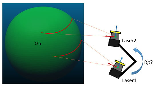
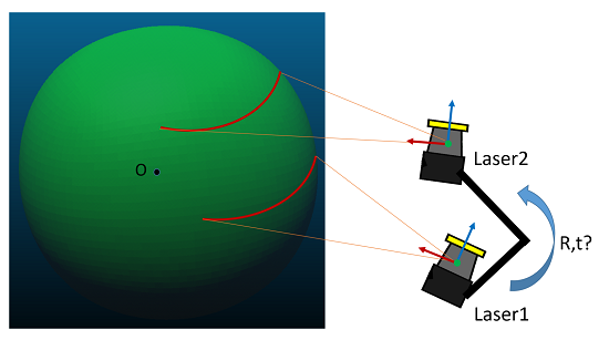
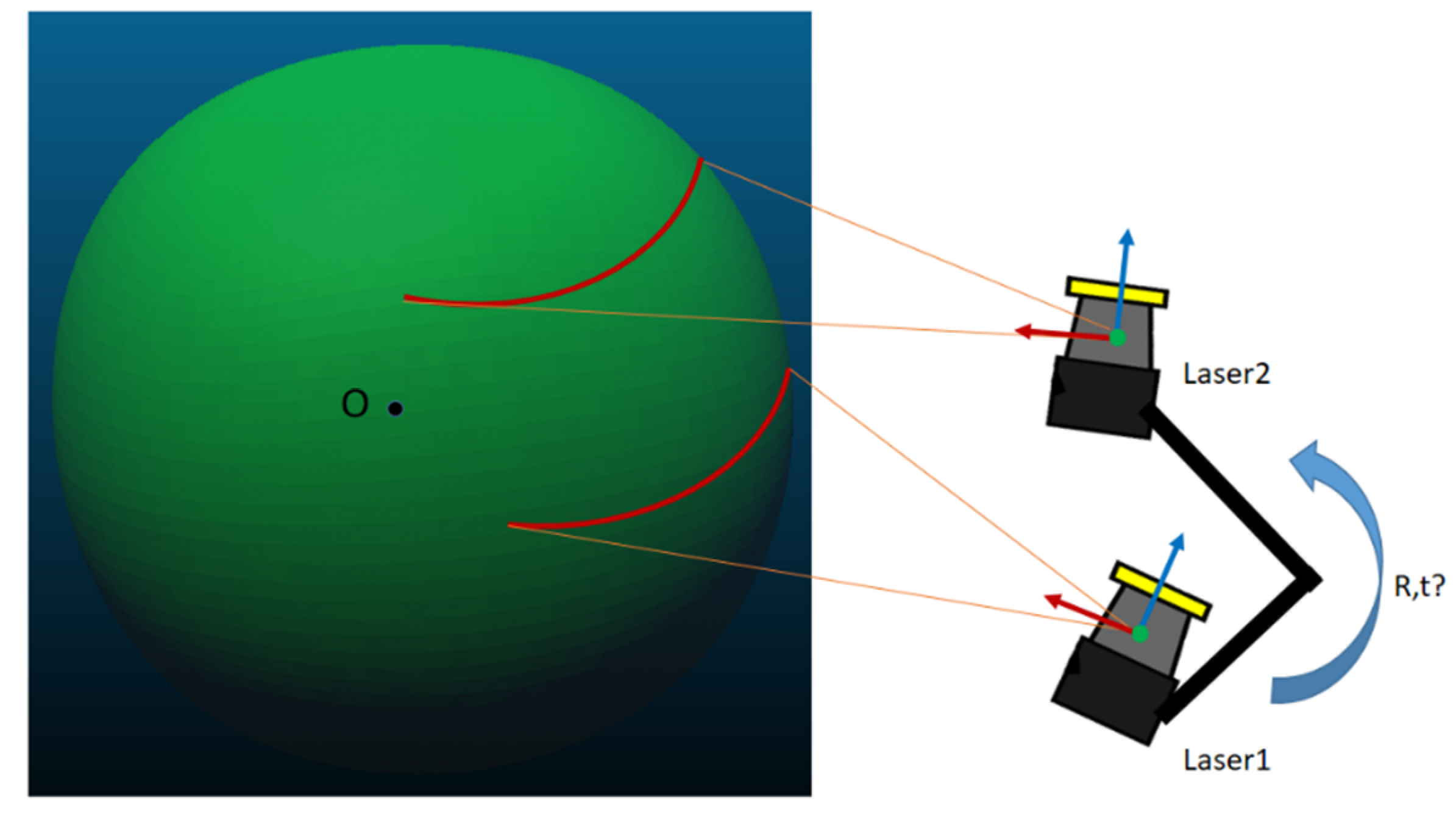
The basic principle of the extrinsic calibration of parameters between multiple 2D LRF sensors is to establish feature correspondences or geometric feature constraints between their observations, and then to estimate the transformation matrix between sensors in a global reference frame. As shown in Figure 1, after two 2D LRFs scan a common three-dimensional spherical target with a known radius, there are two scanning planes containing a circular arc. With the point cloud library (PCL) processing capabilities and the random sample consensus (RANSAC) method, the radius and center of the circle can be modeled, and then the center coordinates of the sphere in the LRF body frame can be extrapolated. Although the scanning planes from the different LRF sensors are different at the same scan timestamp, their calculated spherical centers are still common within the global reference frame, and they become a pair of CPs for the transformation matrix between the two LRF body frames. While constantly moving the spherical target in the common view of the LRFs, we can obtain hundreds of pairs of CPs to establish the calibration equation, which is a least-square problem that can be solved by a closed-form solution based on the singular value decomposition (SVD) or a nonlinear optimization numerical solution based on a least-square bundle adjustment.
2.1. Calculation of the Spherical Center
2.1.1. Point Cloud Filtering
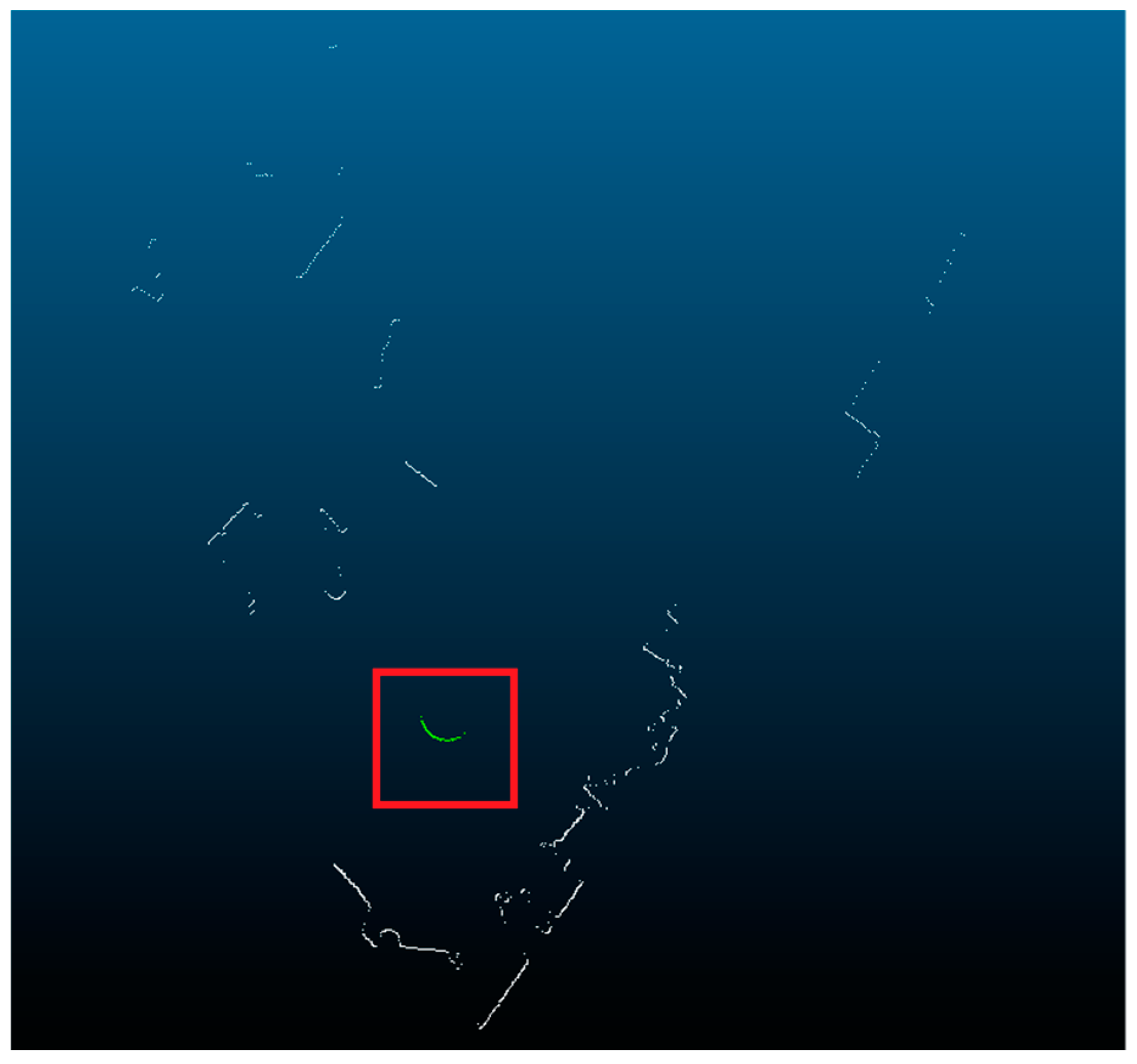
Each scan from an LRF sensor is composed of hundreds or even thousands of 3D points. According to the size of the calibration target and the relative positions between the laser scanners and the sphere, we can establish an appropriate coordinate interval as a filter condition to exclude outlying points far from the circle model. As shown in Figure 2, the red box is the filtering interval, and the white points represent the point cloud before filtering, while the green points represent the point cloud after filtering. This PassThrough filter named by PCL [19] helps exclude outside interference within the scans, which ultimately benefits the next step constituting the fitting of a circle model.
2.1.2. RANSAC Circle Model Fitting
RANSAC is an iterative and nondeterministic algorithm employed to estimate the parameters of a mathematical model from a set of observed data that contains certain outliers [20,21]. Assuming that there is a circular arc within the observations from the 2D LRFs, we can detect the circle model with the RANSAC algorithm. The input to the RANSAC algorithm is the point cloud after the filtering from the previous step, after which the circle model is fitted to the observations; then, we can acquire some reliable properties such as the center coordinates and circle radius. The main steps are as follows:
Step 1. Select a random subset consisting of three noncoplanar points from the input point cloud. Call this subset the hypothetical inliers.
Step 2. A circle model M described by is fitted to the set of hypothetical inliers. The circle center is , and the circle radius is r.
Step 3. All other points are then tested against the fitted model. All points whose distances to the circle center O are less than the circle radius are effectively suitable for the estimated model and are considered a part of the consensus set I.
Step 4. If the number of elements in the current set is greater than that in the optimal set , then update I and the number of iterations.
Step 5. If the number of iterations is greater than an upper limit of iterations k, then exit; otherwise, the number of iterations is increased by 1, and the above steps are repeated. To ensure that the points are selected without replacement, the upper limit can be defined as follows:
where p is the confidence level, which is generally equal to 0.995, w is the probability that a randomly selected single point happens to be an inlier, and m is the minimum number of sample points required for estimating the model and is equal to 3 for the circle model considered here.
2.1.3. Extrapolation of the Spherical Center
After determining the center and radius of the circular arc, it is possible to calculate the spherical center with the known radius R. Because there is a distance between the circle center and the spherical center, the calculation of the spherical center is actually a nonlinear extrapolation process. The distance can be defined as follows:
It is necessary to mention that the confirmation of the hemispheres that belong to the detected circle is ambiguous when using only 2D scans, due to the symmetry of the sphere. To determine whether the Z coordinate of the spherical center is positive or negative, a priori information about the position of the sensor relative to the sphere is required. When the spherical center is above the 2D scanning plane, the coordinates of the spherical center are defined as ; alternatively, when the spherical center is below the 2D scanning plane, the coordinates of the spherical center are defined as .
2.2. CP Matching
At the same timestamp, although the scanning planes from the different LRF sensors are different, their calculated spherical centers are still common within the global reference frame, and they become a pair of CPs for the transformation matrix between the two LRF body frames. While constantly moving the spherical target in the common view of the LRFs, we can match multiple pairs of CPs from multiple observations aligned with the sample timestamp:
where P represents the spherical centers in the Laser1 body frame, P′ represents the spherical centers in the Laser2 body frame, and n represents the number of observations.
It is worth noting that fully synchronous samples are difficult to acquire when using multiple sensors; thus, there is typically a minor difference in the timestamp alignment. According to experimental statistics, the time difference of the majority of CPs is approximately 5 ms, which is one fifth of the sensor scanning time. Moreover, the spherical center is suggested to move as slowly as possible and the speed in our experiment is approximately 0.2 m/s or even lower, close to zero. Therefore, the error caused by the sensor samples being out of sync and the movement of the spherical center is approximately 1 mm (5 ms × 0.2 m/s) or even lower, which is so slight and negligible that we can ignore the effect of the error and regard the low-dynamic collection as approximately the static one.
In addition, there is a significant source of error in the CP matching: the error caused by the extrapolation of the spherical center. The accuracies of both the circle properties and the spherical radius affect the extrapolation accuracy of the spherical center. We define the errors of the circle properties including the radius r and the spherical properties including the radius R as and , respectively. While the errors in the X and Y coordinates are mainly derived from the circle center, which is to say that , the error in the Z coordinate varies along the radius of the circle, r, and the radius of the sphere, R. R and r are uncorrelated, and the total differential equation of (2) is derived as follows:
Based on the law of the propagation of error [22], the error in the Z coordinate is derived as follows:
where and are fixed values determined in the later experiment Section 3, while is a variance related to and , which are the error propagation coefficients that vary with . It is obvious that is a monotonically increasing function of in (5). Based on the relationship between and , selection of a machine with a CP with low error can be established to provide a high-accuracy calibration, and we approximate that after the selection, the detailed analysis of which will be presented in Section 3.3.
2.3. Calibration
2.3.1. Calibration Model
The purpose of the calibration of the extrinsic parameters is to estimate the transformation matrix between sensors in a global reference frame. If a set of pairs of matched CPs completely exists, this issue becomes an Absolute Orientation problem [23,24]. The geometric constraint can be written as (6) for CP pair i:
Then, the point-to-point error is (7):
Equation (7) is the basic calibration model in this paper. The objective is to solve for the rigid transformation matrix T that minimizes the error in the CP pairs. Because of the approximately equal precision of different co-ordinate observations, , and the point-to-point error minimization metric (8) is the objective optimization function of the unweighted least-squares bundle adjustment:
2.3.2. Solution of Equations
For the convenience of taking the derivative of (7), the Lie algebra form of the transformation matrix can be introduced as follows [25,26]:
where is a six-dimensional vector corresponding to the six degrees of freedom of the transformation matrix T, the first dimension is related to translation but does not equal , the last dimension is the Lie algebra of rotation R, and the other terms are intermediate variables described in detail in the Lie algebras and Lie group theory [27].
Then, using to represent the pose and linearization, the error equation can be written as follows:
Based on the Lie algebraic perturbation model, taking the derivative of (10) with respect to can be expressed as follows:
where is the correction for the calibration parameters, and .
Considering different CP pairs, the error equation can be written as:
For convenience, (12) can be simplified into (13):
Equation (13) is the basic error equation, and the corresponding normal equation of (13) is expressed as (14):
The solution of (14) is as follows:
When there are no less than three noncollinear CPs, the transformation parameters can be computed by least-squares adjustment [28]. Some studies have proven that there is a closed-form solution for the least-squares problem, and that the best rigid-body transformation between two coordinate systems can be obtained from measurements of the coordinates of a set of points that are not collinear [24,29,30]. Therefore, a calibration network design with no less than three noncollinear CPs can result in a unique solution and the global optimal solution.
In the transformation parameters, translation has a linear and strong relation with rotation [31], which is derived from the transformation model ubiquitously, not depending on the distribution of CPs. The correlation between the calibration parameters will affect the behavior of the reduced normal equation and can even cause the morbidity of the least-squares normal equations matrix . We can judge the condition of the normal equations matrix as . While is large, the technique of iteration by correcting the characteristic value [32] can be used to solve this problem of morbidity.
2.4. Processing Procedure
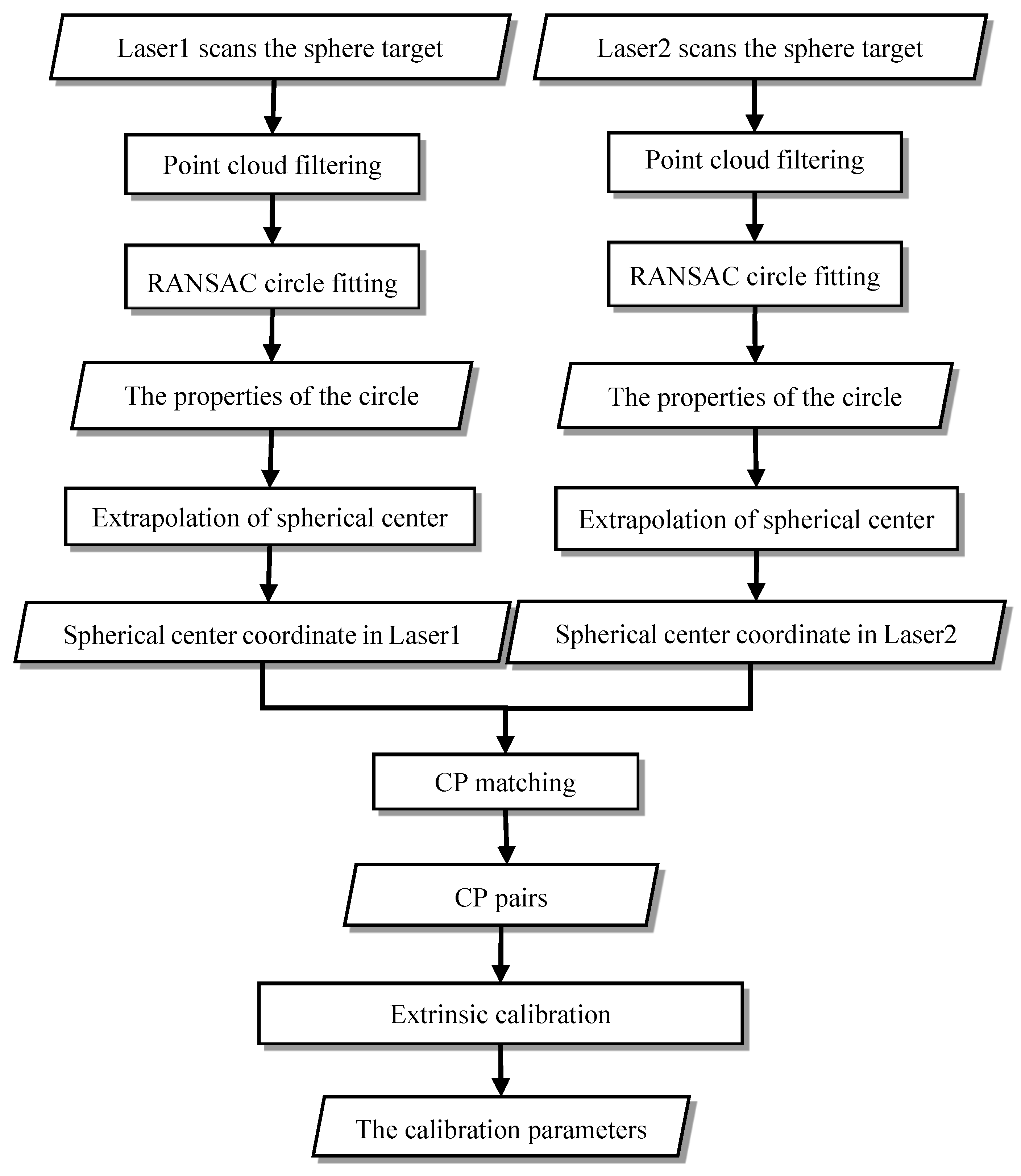
The extrinsic calibration process between Laser1 and Laser2 based on a mobile sphere is shown in Figure 3. There are three main processes: calculation of the spherical center, CP matching, and calibration. The input data are composed of the laser scans reflected by the sphere from the two LRFs, namely, Laser1 and Laser2. The result is the transformation matrix between the Laser1 body frame and the Laser2 body frame.
In the calculation of the spherical center, we need to preprocess the point cloud with an appropriate filter condition and fit the circle model by the RANSAC algorithm requiring the properties (i.e., the center and radius) of the circle. Then, the spherical center is extrapolated based on the geometric relationship with the scan circle center.
Second, by aligning the sample timestamps of Laser1 and Laser2, multiple pairs of CPs can be matched when observing the mobile sphere. Note that fully synchronous samples are impossible to acquire between Laser1 and Laser2 and that out-of-sync sensor samples can cause a slight but unavoidable error in the CP matching.
Finally, the basic calibration model is built based on the geometric constraint of multiple pairs of CPs, after which the calibration equation is solved by a least-square bundle adjustment solution, which results in the calibration parameters. There are many ways to take the derivative; in this paper, the Lie algebraic perturbation model is used for the derivative of the calibration equation.
3. Experiments and Discussion
3.1. Data Introduction
The UTM-30 LX LRF from the Japanese manufacture Hokuyo is an active sensor that emits near-infrared light, which is backscattered from the object surface to the sensor, and it is typically recognized as a time-of-flight ranging system. The Hokuyo UTM-30LX LRF uses pulsed laser light beams to directly measure a time delay created by light traveling from the sensor to the object and back [33].
The Hokuyo UTM-30LX [1,2] shifts a continuously rotating mirror with an angular resolution of 0.25° between each measurement within a few microseconds. With a 270° field of view, the Hokuyo scanner provides 1080 measurements per scan line in 25 ms. The maximum scanning range is 60 m. It is worth noting that the intrinsic accuracy in the depth direction is 10 mm with a scanning range from 0.1 m to 10 m. The Hokuyo UTM-30LX performance parameters are shown in Table 1.
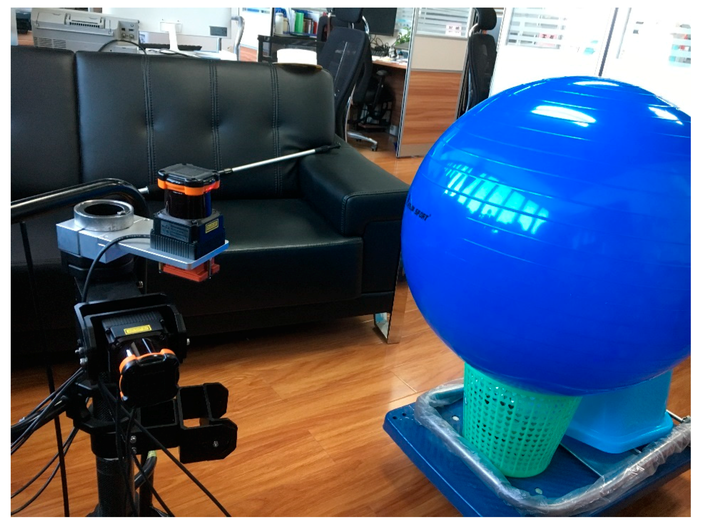
The sphere target employed in the experiment was required to be as accurate as possible, to ensure the accuracy of the calibration. By measurement via terrestrial laser scanning (TLS) RIEGL VZ-400 and sphere fitting of the point cloud, the radius of the mobile sphere target r was 0.325 m, and the fitting precision was 0.003 m, that is, = 0.003 m. The installation configuration of the two Hokuyo UTM-30LX sensors is shown in Figure 4; the Laser1 LRF was assembled horizontally, while the Laser2 LRF was assembled vertically. The positions of the sensor assembly platforms remained unchanged, while the sphere was moved continuously, and the scans from the two sensors were recorded throughout the process.
To address the symmetry of the sphere, that is, to distinguish between the hemispheres along the scan circle, the total CPs were marked as four types depending on the positive or negative direction of the z-axis in the Laser1 and Laser2 body frames: positive-positive CP, positive-negative CP, negative- positive CP, or negative-negative CP. For example, positive-positive CP was located in the positive direction of the z-axis, both in the Laser1 body frame and in the Laser2 body frame. The noncollinear distribution of these CPs must be met in the data collection, and we usually preferred to make CPs distribute in different quadrants and be marked different types.
Moreover, to avoid a poor or morbidity state of the correlation between the calibration parameters, there must be a noncollinear distribution in some of these CPs. This condition was easy to satisfy in the data collection, and we then required a unique and best rigid-body transformation between the two coordinate systems, as mentioned in Section 2.2.
Three datasets in three different configurations of two LRF were collected and used in our experiment. Dataset1 was used as a representative to present the calibration process in detail and to analyze the effect of the CP matching, while in total, three datasets were used for accuracy and robustness validation of this calibration solution. Figure 4 shows the configuration of dataset1, and more detailed information on these datasets and calculated configurations were presented in a later section.
3.2. Circle Model Fitting and the Distribution of CPs
The data about circle model fitting and the distribution of CPs is mainly from dataset1. To prove the efficacy of the point cloud filtering scheme, we conducted a scan at some timestamp from Laser1 as a representative scan. As shown in Figure 2, the red box represented the filter interval condition, while the white and green parts represented the point clouds before and after filtering respectively, indicating that the majority of noise has been removed effectively.
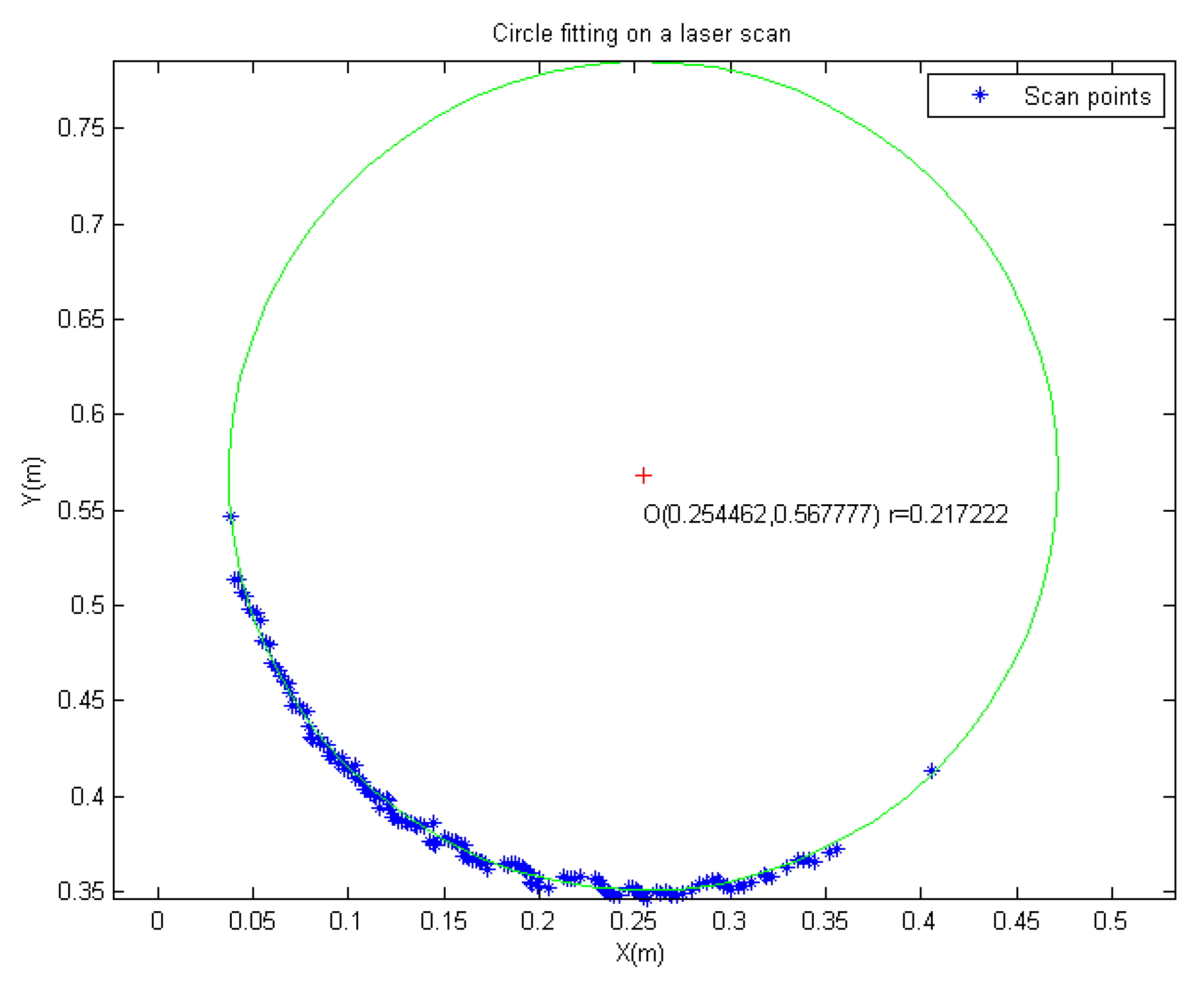
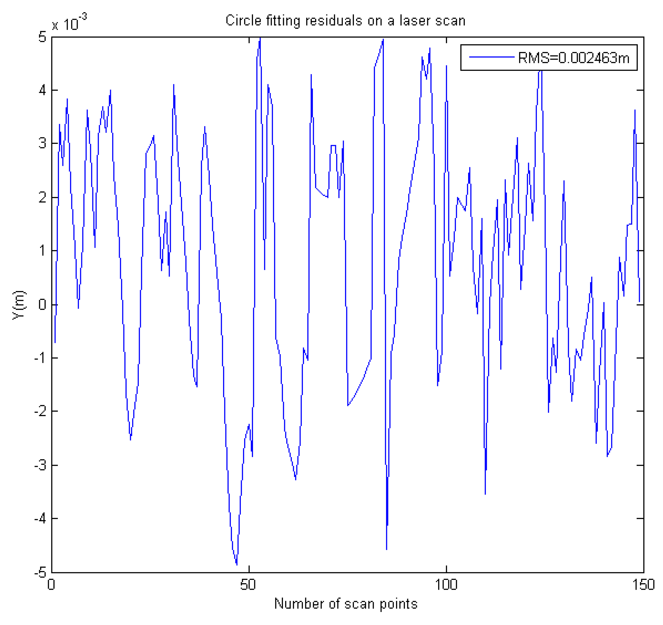
Based on the RANSAC circle detection method described in Section 2.1.2, the result of scanning is shown in Figure 5. There were 149 interior points (blue points) in the circle model (green circle). The fitting residual of each interior sample point was defined as . Figure 6 indicates that the maximum residual error was no more than 0.005 m. Through statistical analysis, the mean value of the residuals was 0.7 mm, and the root-mean-square (RMS) of the residuals was 2.5 mm, which was the RANSAC circle model fitting accuracy. The above index shows that the RANSAC algorithm accuracy in a single scan was high and it satisfied the requirements for the subsequent processes.
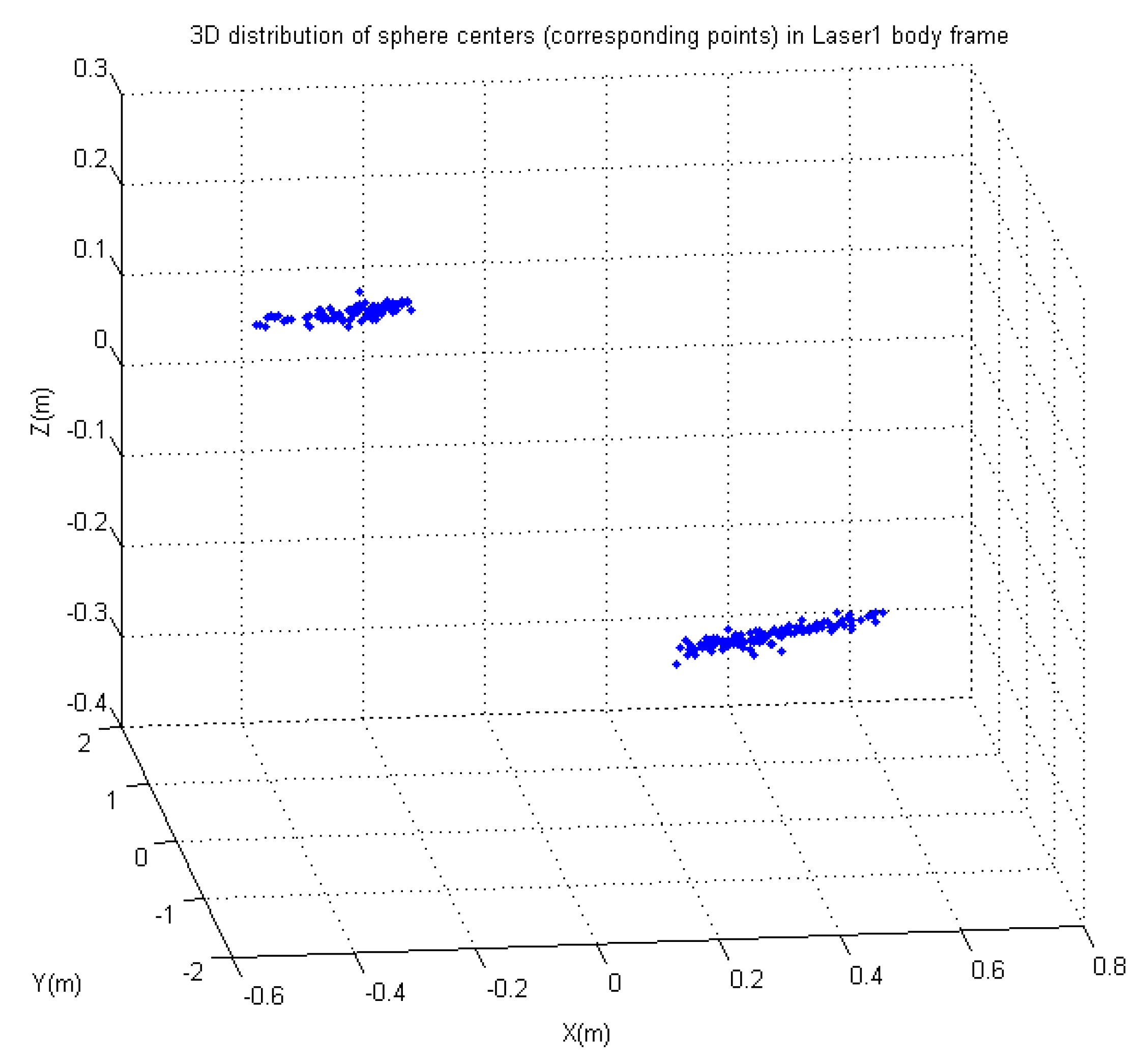
After point cloud filtering, applying the RANSAC circle detection algorithm, and extrapolating the center of the sphere, 308 pairs of CPs could be obtained. Figure 7 shows the distribution of CPs in different quadrants of the Laser1 body coordinate system. It is obvious that these were noncollinear distributions, although there are two short tracks of CPs. The distribution for the Laser2 was similar to the Laser1. Therefore, this dataset had a unique solution and a global optimal solution.
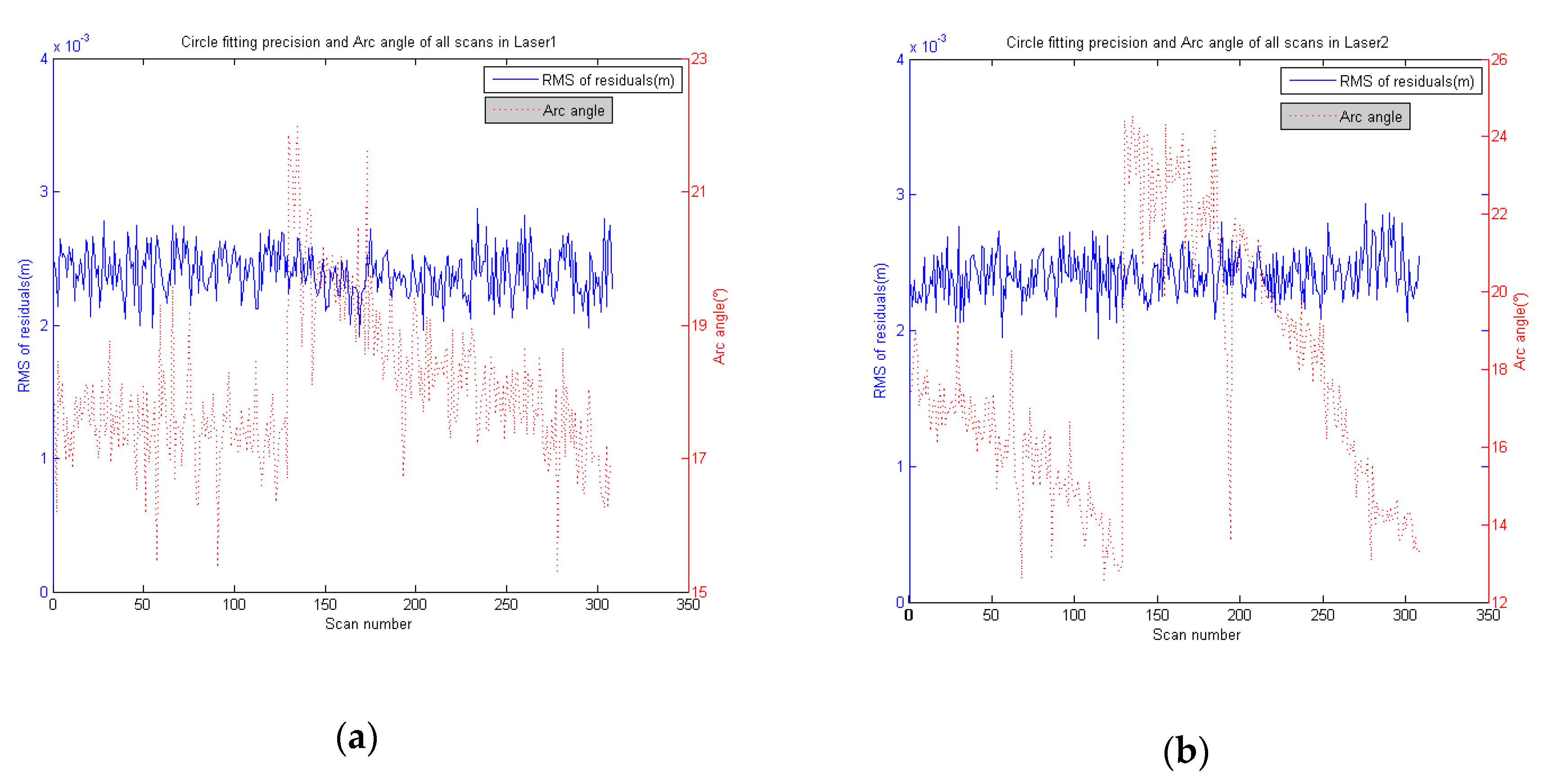
Figure 8 shows the circle fitting accuracies and arc angles for the total scans of Laser1 and Laser2 in dataset1. The circle fitting accuracy was clearly less than 0.003 m. The circle fitting successes and accuracy were consistent, while the arc angle varied, indicating the robustness of the method in function of incompleteness and gap in the measured circle. Combining the circle fitting accuracy with the accuracy of the point cloud in the laser scan, , the accuracies of the center and radius of the circle were evidently maintained at the same level as the intrinsic accuracy , which was also 10 mm.
3.3. Calibration and Analysis
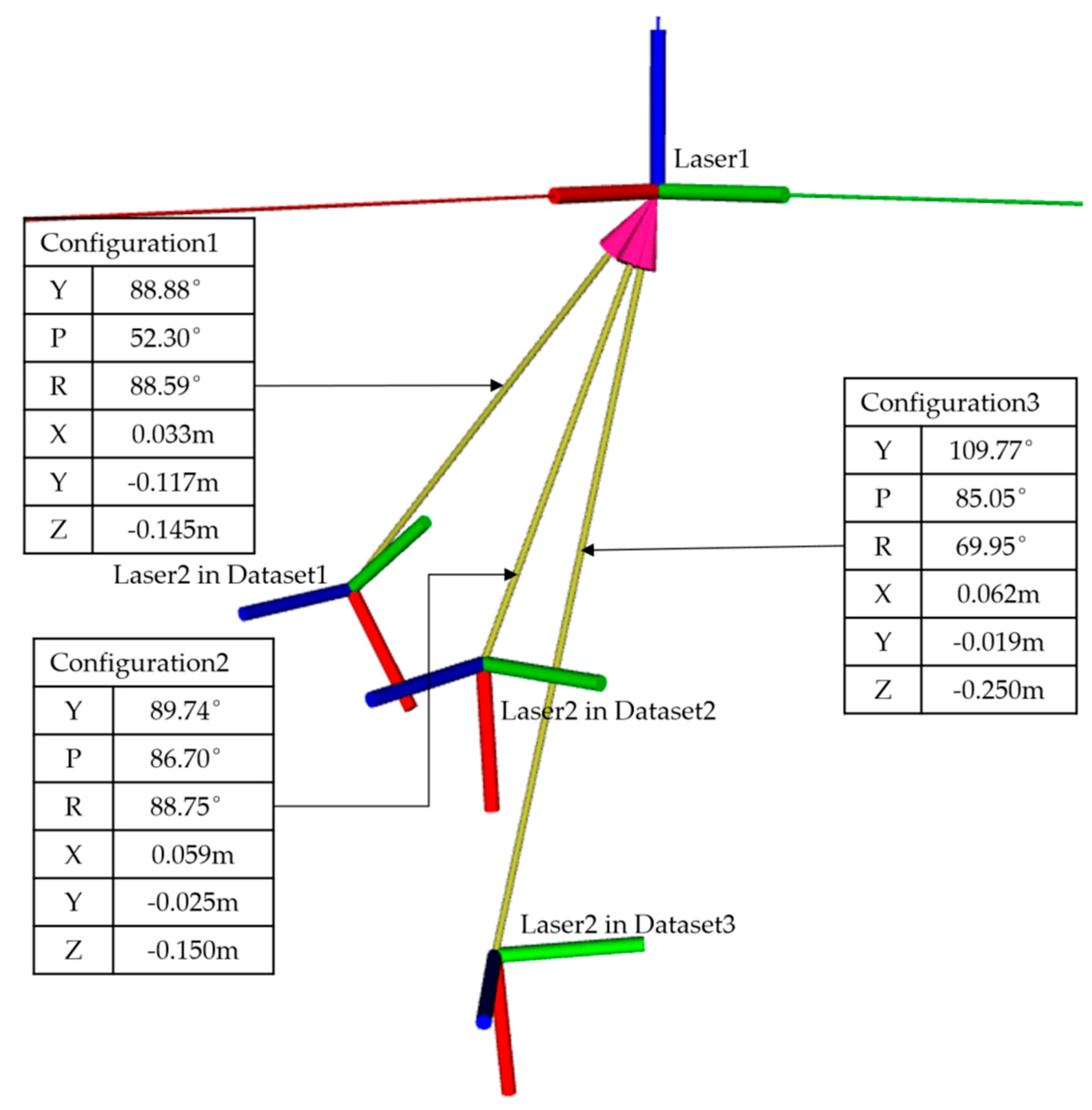
The external parameters of dataset1 calculated according to the calibration model mentioned in Section 2 were translated to an equal and easier interpretation style of Euler extrinsic rotation angles yaw-pitch-roll (YPR) around a fixed Z-Y-X axis (88.88°, 52.30°, 88.59°), and the translation (0.033 m, −0.117 m, −0.145 m), and frames configuration are shown in Section 3.4.
After calculating the calibration parameters via the proposed method, it was important to evaluate the accuracy and conduct an error analysis of the calibration solution. Although ground truth for the relative positions of the sensors can be used to compare the estimated transformation with the exact transformation among the sensors, requiring the availability of ground truth complicates an absolute evaluation of the method. Considering the difficulty involved in precisely measuring the correct pose between a pair of sensors, we cannot guarantee high precision even if the obtained calibration is correct. This problem is particularly difficult with rotations (i.e., it is possible to have a fairly reasonable evaluation of the translation with simple measurements using a measuring tape), which is critical, since small errors in a rotating system may result in large errors within the final registered data.
With this problem in mind, our goal is to perform a calibration of other devices with respect to one reference sensor. Then, the point cloud of the reference sensor is used as the ground truth, and the resulting transformation from the calibration is applied to the remaining sensors. This allows us to evaluate how well the point clouds fit the reference point cloud by calculating the CP residual defined in (7), which represents the exterior orientation accuracy.
The previous solution with a Sick LMS151 sensor in [18] stated the absolute mean error and the standard deviation of the Euclidean distance between CPs. Table 2 shows a comparison between the accuracy of our solution and that of the previous solution. In the previous solution, the value range of was (0, 1), while the absolute mean error and the standard deviation were 68 mm (approximately five times the sensor intrinsic accuracy of 12 mm) and 34 mm (approximately 3 times the sensor intrinsic accuracy of 12 mm), respectively. In our solution, the value range of was (0, ), while the absolute mean error and the standard deviation were12 mm and 14 mm, respectively, which were nearly at the intrinsic accuracy level of the sensor. This contrast indicates that our solution was more accurate than the previous solution, because the CP matched the restriction constraint of the scan circle radius.
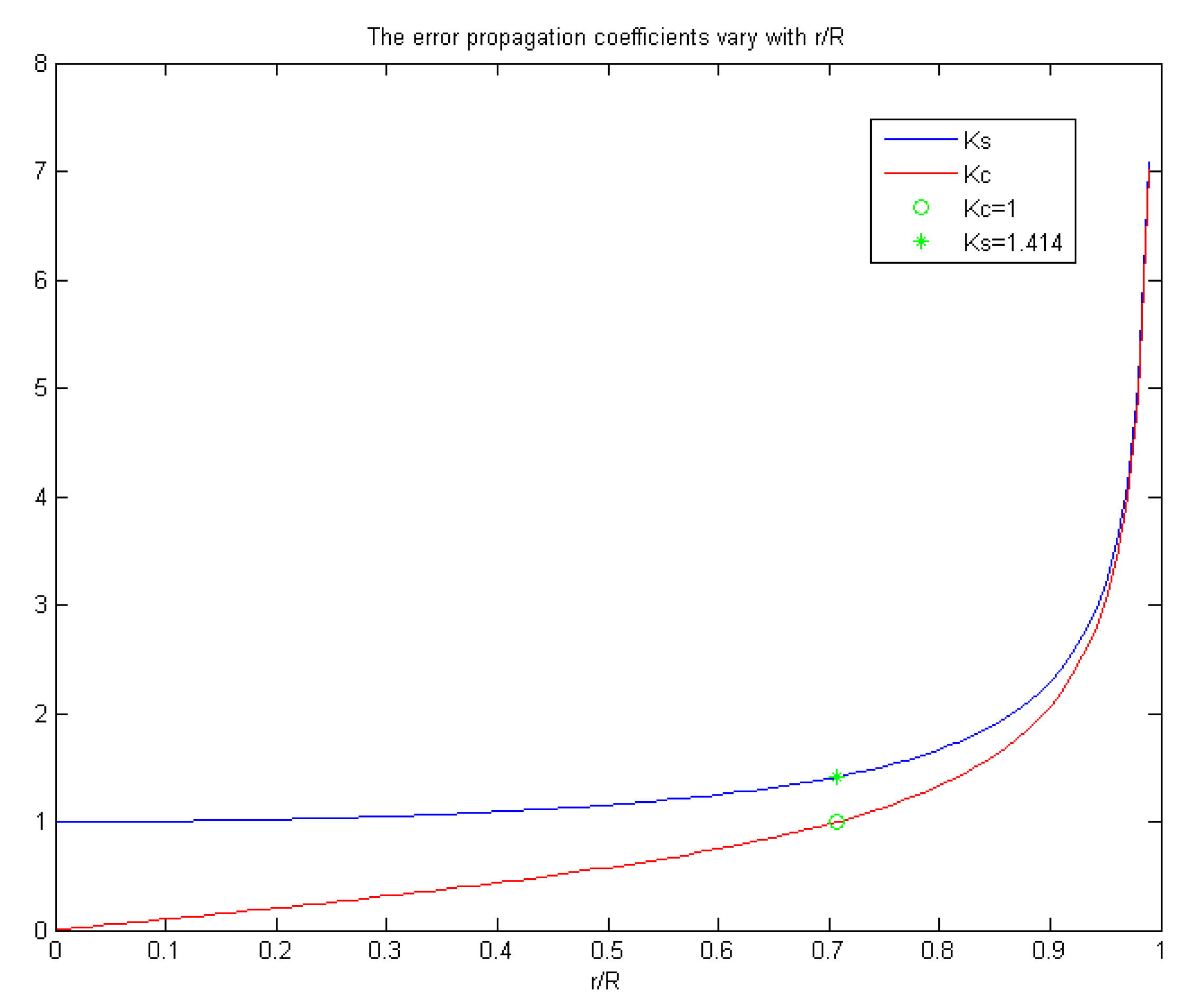
Using the same Hokuyo UTM-30LX sensor, we then further analyzed the influence of . The error propagation coefficients and discussed in Section 2.2 varied with , as shown in Figure 9. Larger values corresponded to larger and values and greater errors in the Z coordinate . In particular, as approached 1, increased dramatically, which was not desirable in the error propagation.
When , then . In this case, the error sourced by the circle radius was not amplified, and the error sourced by the spherical radius was slightly amplified unavoidably. A total of 308 CP pairs composed the first subset, while the second subset was selected according to . The calibration solution was conducted on these two subsets separately.
The external parameters are input into the residual calculation formula, and the resulting statistics are shown in Table 3. The RMS values of the residuals in the second subset were less than those in the first subset. In particular, the RMS values in the Z direction in the second subset were approximately one-third of those in the first subset. The means in all three directions in each subset were each less than 1 × 10⁶ m. In the first subset without any restriction constraint for the scan circle radius, the absolute mean error and the standard deviation both exceeded 0.02 m. While r/R varied from (0, 1) to (0,) between the first and second subsets, the absolute mean error and the standard deviation decreased by approximately one-half, respectively. This contrast indicates that the CP matching with the restriction constraint of the scan circle radius was more accurate and evidently improved orientation accuracy after calibration.
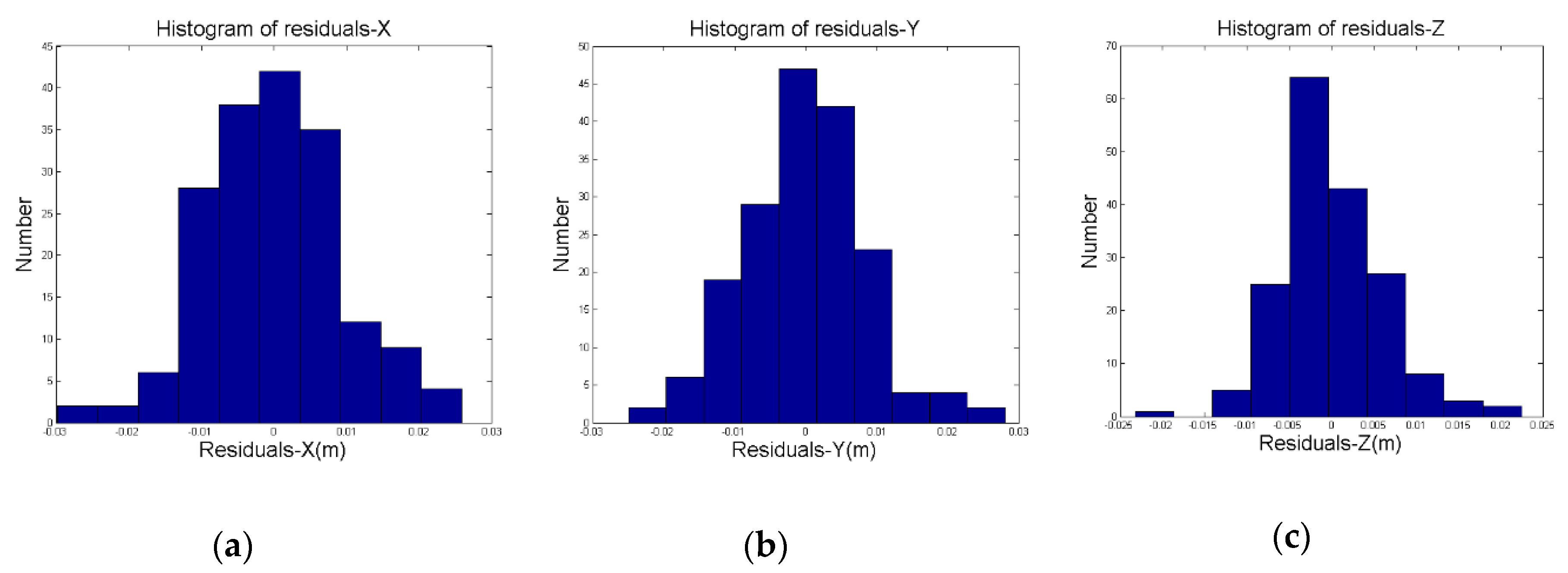
In the second subset with the restriction constraint of the scan circle radius, the mean values of the residuals along each coordinate axis were close to zero, and the RMS values of the residuals were approximately 0.01 m. The residual distribution histogram of the second subset in Figure 10 was similar to a standard normal distribution, which indicates that there was no systematic error after calibration. Therefore, the extrinsic orientation accuracy after calibration was approximately 0.01 m. Considering that the intrinsic accuracy of the Hokuyo UTM-30LX sensor within a range of 10 m was 0.01 m, the calibration parameters acquired in this paper were highly accurate and effective for further application.
3.4. Robustness and Accuracy Validation
To verify the robustness of the calibration solution, three datasets from three different laser frame configurations were collected. Figure 11 shows the laser frame configurations corresponding to the calculated transformation parameters in the three different datasets. The conditions of the normal equations matrix of these three datasets are both approximately 1000, presenting the good behavior of the normal equation in these three datasets.
The calibration parameters of the three datasets are calculated separately. In these three datasets, laser rangefinders are assembled with different rotations and translations, and the calibration accuracies are high, as shown in Table 4. The contrast indicates the robustness of the proposed method in the function of different rotations and translations (frame configuration) of LRFs.
In the situation of difficult access to high-accuracy ground truth, the accuracy validation of the calibrated system is actually the evaluation of point clouds. According to [8], the evaluation of point clouds can be roughly divided into three approaches: the control point approach, the subset approach and the full point cloud approach. Calculating the residuals of the CPs is a classical method to assess the calibration accuracy [18], which belongs to the control point approach.
The total CP residuals in Section 3.2 reflected the exterior orientation accuracy to some extent, but it was insufficient. To further verify the accuracy of the calibration parameters, the CPs in every dataset were randomly divided into two sections: training points and test points. Training points are mainly used to calculate and estimate the calibration parameters, while test points independent of the calibration mainly verify the generation of the calibration parameters. Orientation accuracies of the training points and test points in the three datasets are shown in Table 4.
In these three datasets, the mean values of the residuals for the training points and test points were both close to zero. Although the level of the mean values for the test points was 1 × 10⁻⁴, which was less than that for the training points at 1 × 10⁻⁷, it still demonstrated the high accuracy of the extrinsic orientation, considering the error of CPs caused by the intrinsic accuracy of the Hokuyo UTM-30LX sensor. In terms of the RMS values of the residuals, the test points and training points in the three datasets performed consistently in all three directions at the level of approximately 0.01 m. The results verified the correctness of the calibration parameters, and the extrinsic orientation accuracy after calibration was approximately 0.01 m.
In addition, we tried other two approaches as a supplementary. The full point cloud approach can be used to evaluate the calibrated system of the 3D laser scanners. However, in our calibrated system composed by two 2D LRFs, there only two scan lines and it was difficult to compare the two scan lines with the 3D point cloud from the TLS. Therefore, we had to employ the subset approach as a supplementary method to verify the correctness of our calibration parameters, and the subset of points including a specific geometric feature can be extracted and compared to the data from the TLS.
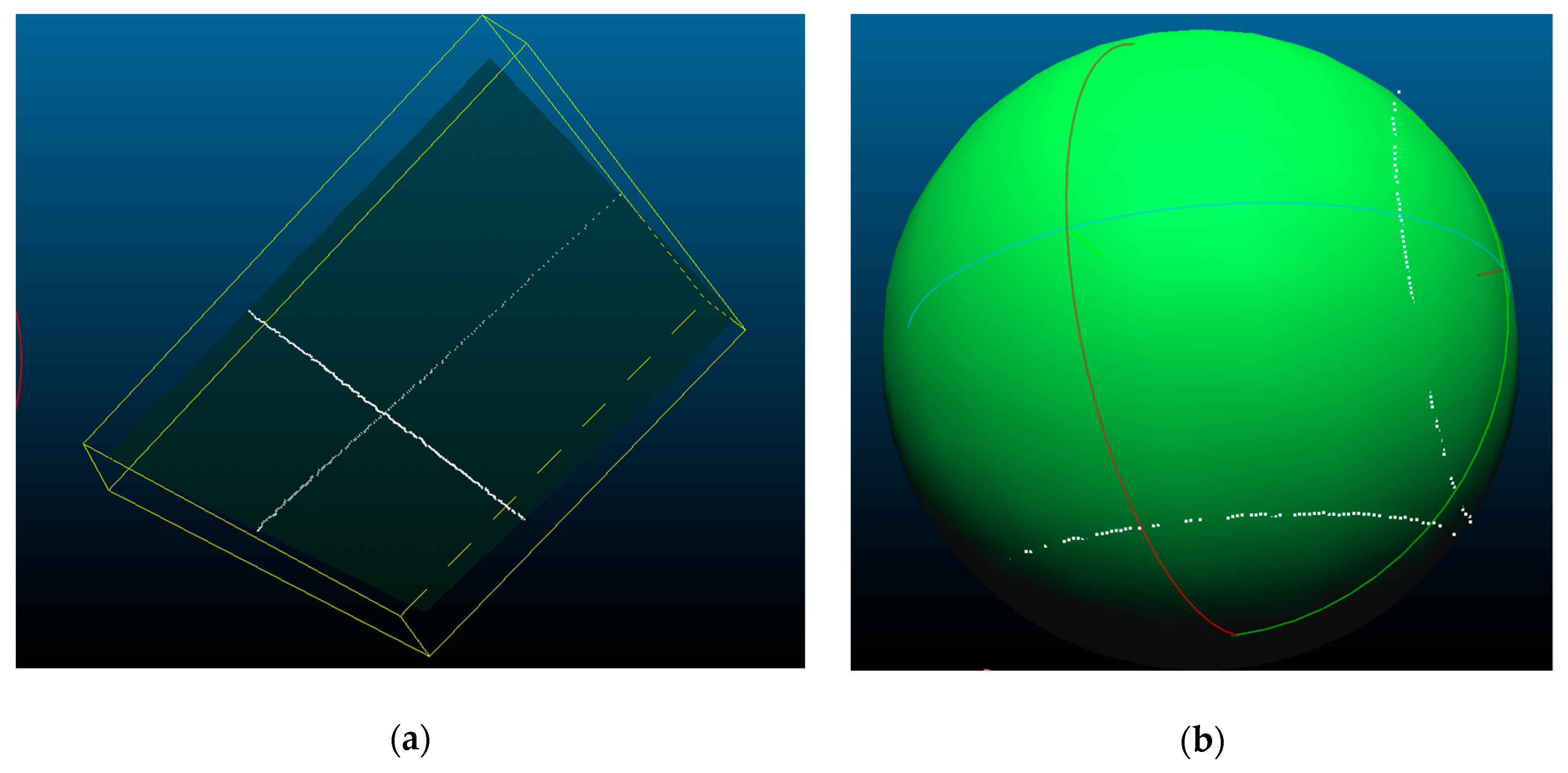
In the practical experiment, a 2D scene of a flat wall and a 3D scene of the calibration sphere were selected for scanning by our sensor platform. The indoor decoration standard [34] states that the flatness of the wall is less than 4 mm, and the plane fitting precision in this scene is actually very high at only 1.2 mm by measurements from the TLS RIEGL VZ-400. The performances of the sphere were measured by the TLS in Section 3.1. Based on the Laser1 body coordinate system, the point cloud in the Laser2 system was transformed into the reference coordinate system using the transformation matrix of dataset1 acquired by the proposed method. The result of the point cloud is shown in Figure 12, where the green part represents the wall or the spherical target. The wall was segmented, and the plane fitting error was 8.085 mm, which was less than 10 mm. The spherical radius and the spherical fitting error of our calibrated system were 0.326 m and 3 mm. This was consistent with the intrinsic accuracy of the LRF. In conclusion, the calibration method in this paper is effective and meets the requirements of practical measurements.
4. Conclusions
This paper presents a methodology for calibrating the extrinsic parameters of a combination of 2D LRF sensors based on a mobile sphere. The proposed method boasts an automatic and high-accuracy solution. Moreover, establishing a CP matching machine with the restriction constraint of the scan circle radius is established. Experiments using the Hokuyo UTM-30LX sensor show that the method can match CPs with a low error and improve the orientation accuracy level to 0.01 m, which is consistent with the intrinsic accuracy of the Hokuyo UTM-30LX sensor. This result indicates that the calibration method in this paper is effective and meets the requirements of practical measurements.
In addition, due to the symmetry of the sphere, an a priori parameter, namely, the relative position between the laser scanner and the spherical target (i.e., whether it is placed above or below its equator), is required. In the future, we plan to conduct some research to resolve all ambiguities corresponding to the positions of the sensors insomuch that they do not require a priori information regarding their positions relative to the hemisphere.
Author Contributions
S.C. wrote the paper and conducted the experiments. J.L. guided the structure of the paper. T.W. and W.H. gave some suggestions. K.L. and D.Y. helped with the data acquisition. X.L., J.H. and R.C. proofread and checked the paper.
Acknowledgments
This study was supported in part by the National Key Research Development Program of China with project No. 2016YFE0202300, the Technology Innovation Program of Hubei Province with Project No. 2018AAA070, and the Natural Science Fund of Hubei Province with Project No. 2018CFA007.
Conflicts of Interest
The authors declare no conflicts of interest.
References
- Scanning Range Finder Utm-30lx Product Page. Available online: http://www.hokuyo-aut.jp/02sensor/07scanner/utm_30lx.html (accessed on 20 April 2018).
- Pouliot, N.; Richard, P.L.; Montambault, S. Linescout power line robot: Characterization of a utm-30lx lidar system for obstacle detection. In Proceedings of the IEEE/RSJ International Conference on Intelligent Robots and Systems, Vilamoura, Portugal, 24 December 2012; pp. 4327–4334. [Google Scholar]
- Demski, P.; Mikulski, M.; Koteras, R. Characterization of Hokuyo Utm-30lx Laser Range Finder for an Autonomous Mobile Robot; Springer: Heidelberg, Germany, 2013; pp. 143–153. [Google Scholar]
- Mader, D.; Westfeld, P.; Maas, H.G. An integrated flexible self-calibration approach for 2d laser scanning range finders applied to the Hokuyo utm-30lx-ew. ISPRS Int. Arch. Photogramm. Remote Sens. Spat. Inf. Sci. 2014, 5, 385–393. [Google Scholar] [CrossRef]
- Navvis Digitizing Indoors—Navvis. Available online: http://www.navvis.com (accessed on 20 April 2018).
- Google Cartographer Backpack. Available online: https://opensource.google.com/projects/cartographer (accessed on 20 April 2018).
- Hess, W.; Kohler, D.; Rapp, H.; Andor, D. Real-time loop closure in 2d lidar slam. In Proceedings of the IEEE International Conference on Robotics and Automation, Stockholm, Sweden, 16–21 May 2016; pp. 1271–1278. [Google Scholar]
- Lehtola, V.V.; Kaartinen, H.; Nüchter, A.; Kaijaluoto, R.; Kukko, A.; Litkey, P.; Honkavaara, E.; Rosnell, T.; Vaaja, M.T.; Virtanen, J.P. Comparison of the selected state-of-the-art 3d indoor scanning and point cloud generation methods. Remote Sens. 2017, 9, 796. [Google Scholar] [CrossRef]
- Lehtola, V.V.; Virtanen, J.P.; Kukko, A.; Kaartinen, H.; Hyyppä, H. Localization of mobile laser scanner using classical mechanics. ISPRS J. Photogramm. Remote Sens. 2015, 99, 25–29. [Google Scholar] [CrossRef]
- Zhang, J.; Singh, S. Loam: Lidar odometry and mapping in real-time. In Proceedings of the Robotics: Science and Systems Conference, Berkeley, CA, USA, 12–16 July 2014. [Google Scholar]
- Fernández-Moral, E.; González-Jiménez, J.; Arevalo, V. Extrinsic calibration of 2d laser rangefinders from perpendicular plane observations. I. J. Robot. Res. 2015, 34, 1401–1417. [Google Scholar] [CrossRef]
- Levinson, J.; Askeland, J.; Becker, J.; Dolson, J.; Held, D.; Kammel, S.; Kolter, J.Z.; Langer, D.; Pink, O.; Pratt, V. Towards fully autonomous driving: Systems and algorithms. In Proceedings of the Intelligent Vehicles Symposium, Baden-Baden, Germany, 5–9 June 2011; pp. 163–168. [Google Scholar]
- Miller, I.; Campbell, M.; Huttenlocher, D. Efficient unbiased tracking of multiple dynamic obstacles under large viewpoint changes. IEEE Trans. Robot. 2011, 27, 29–46. [Google Scholar] [CrossRef]
- Leonard, J.; How, J.; Teller, S.; Berger, M.; Campbell, S.; Fiore, G.; Fletcher, L.; Frazzoli, E.; Huang, A.; Karaman, S. A perception-driven autonomous urban vehicle. J. Field Robot. 2008, 25, 727–774. [Google Scholar] [CrossRef] [Green Version]
- Huang, A.S.; Antone, M.; Olson, E.; Fletcher, L.; Moore, D.; Teller, S.; Leonard, J. A high-rate, heterogeneous data set from the darpa urban challenge. Int. J. Robot. Res. 2010, 29, 1595–1601. [Google Scholar] [CrossRef] [Green Version]
- Gao, C.; Spletzer, J.R. On-line calibration of multiple lidars on a mobile vehicle platform. In Proceedings of the IEEE International Conference on Robotics and Automation, Anchorage, AK, USA, 3–7 May 2010; pp. 279–284. [Google Scholar]
- Underwood, J.; Hill, A.; Scheding, S. Calibration of range sensor pose on mobile platforms. In Proceedings of the IEEE/RSJ International Conference on Intelligent Robots and Systems, San Diego, CA, USA, 29 October–2 November 2007; pp. 3866–3871. [Google Scholar]
- Pereira, M.; Silva, D.; Santos, V.; Dias, P. Self calibration of multiple lidars and cameras on autonomous vehicles. Robot. Auton. Syst. 2016, 83, 326–337. [Google Scholar] [CrossRef]
- Pcl Turorials: Filtering a Pointcloud Using a Passthrough Filter. Available online: http://www.pointclouds.org/documentation/tutorials/passthrough.php#passthrough (accessed on 15 June 2018).
- Meng, Y.; Zhang, H. Registration of point clouds using sample-sphere and adaptive distance restriction. Vis. Comput. 2011, 27, 543–553. [Google Scholar] [CrossRef]
- Fischler, M.A.; Bolles, R.C. Random Sample Consensus: A Paradigm for Model Fitting with Applications to Image Analysis and Automated Cartography; ACM: New York, NY, USA, 1981; pp. 726–740. [Google Scholar]
- Draper, D. Assessment and propagation of model uncertainty. J. R. Stat. Soc. 1995, 57, 45–97. [Google Scholar]
- Horn, B.K.P. Closed-form solution of absolute orientation using unit quaternions. J. Opt. Soc. Am. A 1987, 5, 1127–1135. [Google Scholar] [CrossRef]
- Arun, K.S.; Huang, T.S.; Blostein, S.D. Least-squares fitting of two 3-d point sets. IEEE Trans. Pattern Anal. Mach. Intell. 1987, 9, 698–700. [Google Scholar] [CrossRef] [PubMed]
- Barfoot, T.D. A matrix lie group approach. In State Estimation for Robotics; Cambridge University Press: Cambridge, UK, 2017. [Google Scholar]
- Hassani, S. Representation of Lie Groups and Lie Algebras; Springer International Publishing: Basel, Switzerland, 2013; pp. 953–985. [Google Scholar]
- Varadarajan, V.S. Lie Groups, Lie Algebras, and Their Representations; Springer: New York, NY, USA, 1974. [Google Scholar]
- Umeyama, S. Least-squares estimation of transformation parameters between two point patterns. IEEE Trans. Pattern Anal. Mach. Intell. 1991, 13, 376–380. [Google Scholar] [CrossRef]
- Jiang, G.W.; Wang, J.; Zhang, R. A close-form solution of absolute orientation using unit quaternions. J. Zhengzhou Inst. Surv. Mapp. 2007, 3, 193–195. [Google Scholar]
- Sharp, G.C.; Lee, S.W.; Wehe, D.K. Icp registration using invariant features. IEEE Trans. Pattern Anal. Mach. Intell. 2002, 24, 90–102. [Google Scholar] [CrossRef]
- Du, L.; Zhang, H.; Zhou, Q.; Wang, R. Correlation of coordinate transformation parameters. Geod. Geodyn. 2012, 3, 34–38. [Google Scholar]
- Wang, X.; Liu, D.; Zhang, Q.; Huang, H. The iteration by correcting characteristic value and its application in surveying data processing. J. Heilongjiang Inst. Technol. 2001, 15, 3–6. [Google Scholar]
- Vosselman, G.; Maas, H.G. Airborne and Terrestrial Laser Scanning. International Journal of Digital Earth. 2010, 4, 183–184. [Google Scholar]
- Ministry of Housing and Urban-Rural Development of the People’s Republic of China. Code for Design of the Residential Interior Decoration; China Architecture & Building Press: Beijing, China, 2015.
Figure 1.
Observation of a sphere by a combination of two laser rangefinders (LRFs). The red scans reflected by the sphere are from the different LRF body frames, and the spherical center O is the common point for establishing the corresponding points (CPs). Assuming that the Laser1 body frame is a global reference frame, the transformation parameters (R, t) between the two LRF body frames can be solved by extrinsic calibration.

Figure 2.
Point cloud filtering preprocessing. The red box is the filtering interval, and the white points represent the point cloud before filtering, while the green points represent the point cloud after filtering.
Figure 2.
Point cloud filtering preprocessing. The red box is the filtering interval, and the white points represent the point cloud before filtering, while the green points represent the point cloud after filtering.

Figure 3.
Extrinsic calibration process between Laser1 and Laser2 based on a mobile sphere. Step 1: calculation of the spherical center, including point cloud filtering, random circle consensus (RANSAC) circle fitting and extrapolation of the spherical center. Step 2: CP matching based on the sample timestamp alignment. Step 3: establishing and solving the extrinsic calibration model.

Figure 4.
Sensor assembly platform and mobile sphere. The Laser1 LRF is assembled horizontally, and the Laser2 LRF is assembled vertically. The radius of the mobile spherical target is 0.325 m.
Figure 4.
Sensor assembly platform and mobile sphere. The Laser1 LRF is assembled horizontally, and the Laser2 LRF is assembled vertically. The radius of the mobile spherical target is 0.325 m.

Figure 5.
Circle fitting on a laser scan. The number of interior points (blue points) in the circle model (green circle) is 149.
Figure 5.
Circle fitting on a laser scan. The number of interior points (blue points) in the circle model (green circle) is 149.

Figure 6.
Circle fitting residuals on a laser scan. The maximum residual error is no more than 0.005 m. The root mean square (RMS) of the residuals is 2.5 mm.
Figure 6.
Circle fitting residuals on a laser scan. The maximum residual error is no more than 0.005 m. The root mean square (RMS) of the residuals is 2.5 mm.

Figure 7.
Non-collinear distribution of CPs in the Laser1 body coordinate system.

Figure 8.
(a) The circle fitting accuracy and arc angle for all scans of Laser1. (b) The circle fitting accuracy for all scans of Laser2.
Figure 8.
(a) The circle fitting accuracy and arc angle for all scans of Laser1. (b) The circle fitting accuracy for all scans of Laser2.

Figure 9.
Error propagation coefficients. The blue line represents the variability of Ks with r/R; the red line represents the variability of Kc with r/R. The green dot is located at (0.707, 1) along the red line; the green crosshair is located at (0.707, 1.414) along the blue line.
Figure 9.
Error propagation coefficients. The blue line represents the variability of Ks with r/R; the red line represents the variability of Kc with r/R. The green dot is located at (0.707, 1) along the red line; the green crosshair is located at (0.707, 1.414) along the blue line.

Figure 10.
Residual distribution histogram of the CPs after calibration. (a) Residual distribution histogram in the X direction. (b) Residual distribution histogram in the Y direction; (c) Residual distribution histogram in the Z direction.
Figure 10.
Residual distribution histogram of the CPs after calibration. (a) Residual distribution histogram in the X direction. (b) Residual distribution histogram in the Y direction; (c) Residual distribution histogram in the Z direction.

Figure 11.
The laser frame configurations corresponding to the calculated transformation parameters in three different datasets, which is defined by a six dimensional vector including Euler extrinsic rotation angles YPR around a fixed Z-Y-X (blue-green-red) axis and the translation.
Figure 11.
The laser frame configurations corresponding to the calculated transformation parameters in three different datasets, which is defined by a six dimensional vector including Euler extrinsic rotation angles YPR around a fixed Z-Y-X (blue-green-red) axis and the translation.

Figure 12.
Validation of the point cloud. (a) The green part is the wall with the accuracy 1.2 mm measured by terrestrial laser scanning (TLS), and the plane fitting error of our calibrated system is 8.085 mm. (b) The green part is the sphere with the radius of 0.325 m and the accuracy of 3 mm measured by TLS, and the spherical radius and the spherical fitting error of our calibrated system are 0.326 m and 3 mm.


Table 1.
Hokuyo UTM-30LX performance parameter table. The intrinsic accuracy is 10 mm with a scanning range from 0.1 m to 10 m.
Table 1.
Hokuyo UTM-30LX performance parameter table. The intrinsic accuracy is 10 mm with a scanning range from 0.1 m to 10 m.
| Item | Technology Performance |
|---|---|
| Measurement Principle | Time of Flight |
| Light Source | Laser Semiconductor λ = 905 nm Laser Class 1 |
| Detection Range | Guaranteed Range: 0.1~30 m (White Kent Sheet) Maximum Range: 0.1~60 m |
| Detection Object | Minimum Detectable Width at 10 m: 130 mm (varies with distance) |
| Measurement Resolution | 1 mm |
| Intrinsic Accuracy(Precision) | 0.1–10 m: σ < 10 mm 10–30 m: σ < 30 mm (White Kent Sheet) Under 3000 lx: σ < 10 mm (White Kent Sheet up to 10 m) Under 100,000 lx: σ < 30 mm (White Kent Sheet up to 10 m) |
| Scan Angle | 270° |
| Angular Resolution | 0.25° (360°/1440) |
| Scan Speed | 25 ms (motor speed: 2400 rpm) |
Table 2.
Accuracy comparison with the previous solution.
| Sensor | Intrinsic Accuracy (mm) | Absolute Mean Error (mm) | Standard Deviation (mm) | ||
|---|---|---|---|---|---|
| Previous Solution | Sick LMS151 | 12 | (0, 1) | 68 | 34 |
| Our Solution | Hokuyo UTM-30LX | 10 | (0, ) | 12 | 14 |
Table 3.
Orientation accuracies in the two subsets of dataset1. The RMS of the Euclidean metric equals the absolute mean error in Table 2. The mean of the Euclidean metric equals the standard deviation in Table 2.
| Subset | CP Pairs | RMS (m) | Mean (m) | |||||||
|---|---|---|---|---|---|---|---|---|---|---|
| X | Y | Z | Euclidean Metric | X | Y | Z | Euclidean Metric | |||
| 1st | 308 | (0, 1) | 0.0147 | 0.0119 | 0.0171 | 0.0255 | 2 × 10⁸ | 7 × 10⁹ | 5 × 10⁸ | 0.0213 |
| 2nd | 178 | (0, ) | 0.0092 | 0.0086 | 0.0060 | 0.0140 | 2 × 10⁷ | 1 × 10⁷ | −3 × 10⁸ | 0.0121 |
Table 4.
Orientation accuracies of the training points and test points in the three datasets.
| Dataset | Point | RMS (m) | Mean (m) | |||||||
|---|---|---|---|---|---|---|---|---|---|---|
| Type | Number | X | Y | Z | Euclidean Metric | X | Y | Z | Euclidean Metric | |
| 1 | Training | 99 | 0.0102 | 0.0087 | 0.0063 | 0.0148 | −2.9 × 10⁻⁸ | −3.5 × 10⁻⁹ | −6.2 × 10⁻⁹ | 0.0129 |
| Test | 98 | 0.0090 | 0.0087 | 0.0071 | 0.0144 | 3.0 × 10⁻⁴ | −4.0 × 10⁻⁴ | −9.0 × 10⁻⁴ | 0.0123 | |
| 2 | Training | 814 | 0.0061 | 0.0118 | 0.0054 | 0.0144 | −7.1 × 10⁻⁹ | −2.4 × 10⁻⁷ | −2.7 × 10⁻⁷ | 0.0130 |
| Test | 814 | 0.0059 | 0.0123 | 0.0053 | 0.0147 | −1.4 × 10⁻⁴ | 2.4 × 10⁻⁴ | 1.4 × 10⁻⁴ | 0.0133 | |
| 3 | Training | 755 | 0.0058 | 0.0112 | 0.0050 | 0.0135 | 1.5 × 10⁻⁸ | −7.6 × 10⁻⁹ | −2.2 × 10⁻⁸ | 0.0120 |
| Test | 755 | 0.0062 | 0.0150 | 0.0052 | 0.0141 | 3.3 × 10⁻⁴ | −4.8 × 10⁻⁴ | −1.9 × 10⁻⁴ | 0.0125 | |
© 2018 by the authors. Licensee MDPI, Basel, Switzerland. This article is an open access article distributed under the terms and conditions of the Creative Commons Attribution (CC BY) license (http://creativecommons.org/licenses/by/4.0/).
Share and Cite
MDPI and ACS Style
Chen, S.; Liu, J.; Wu, T.; Huang, W.; Liu, K.; Yin, D.; Liang, X.; Hyyppä, J.; Chen, R. Extrinsic Calibration of 2D Laser Rangefinders Based on a Mobile Sphere. Remote Sens. 2018, 10, 1176. https://doi.org/10.3390/rs10081176
AMA Style
Chen S, Liu J, Wu T, Huang W, Liu K, Yin D, Liang X, Hyyppä J, Chen R. Extrinsic Calibration of 2D Laser Rangefinders Based on a Mobile Sphere. Remote Sensing. 2018; 10(8):1176. https://doi.org/10.3390/rs10081176
Chicago/Turabian StyleChen, Shoubin, Jingbin Liu, Teng Wu, Wenchao Huang, Keke Liu, Deyu Yin, Xinlian Liang, Juha Hyyppä, and Ruizhi Chen. 2018. "Extrinsic Calibration of 2D Laser Rangefinders Based on a Mobile Sphere" Remote Sensing 10, no. 8: 1176. https://doi.org/10.3390/rs10081176
Note that from the first issue of 2016, this journal uses article numbers instead of page numbers. See further details here.