The Transferability of Random Forest in Canopy Height Estimation from Multi-Source Remote Sensing Data


Abstract
:1. Introduction
2. Data
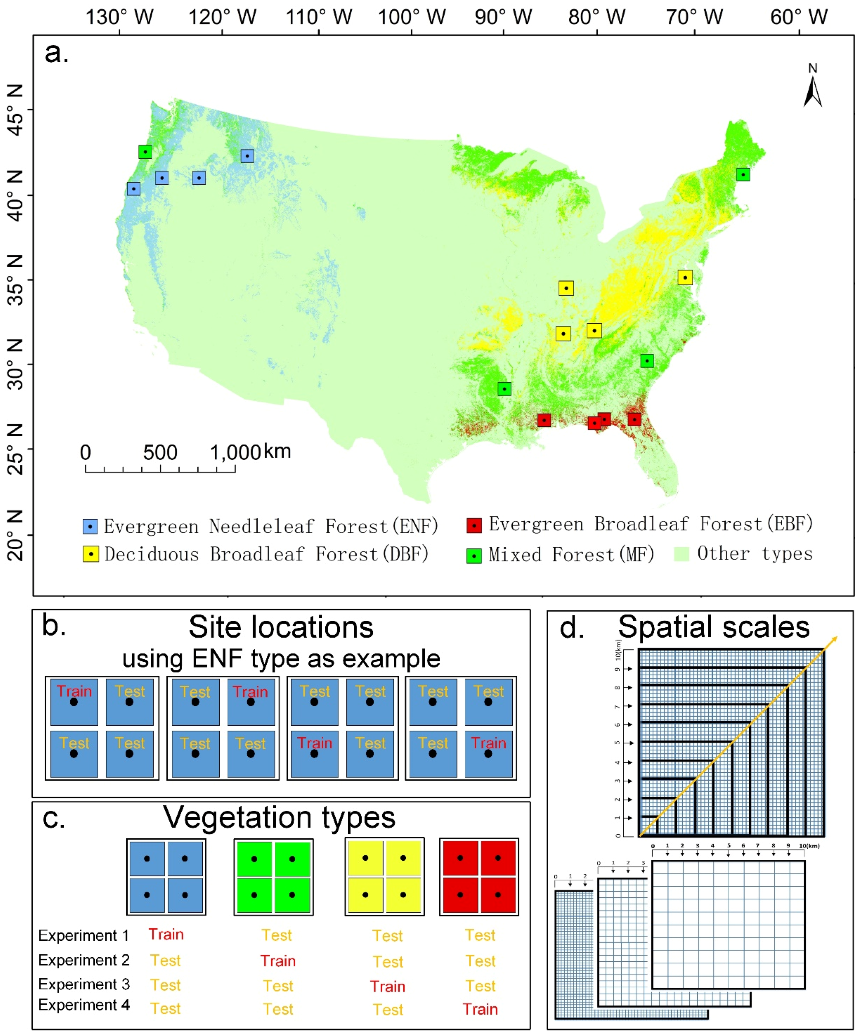
2.1. Study Area
2.2. Airborne LiDAR Data
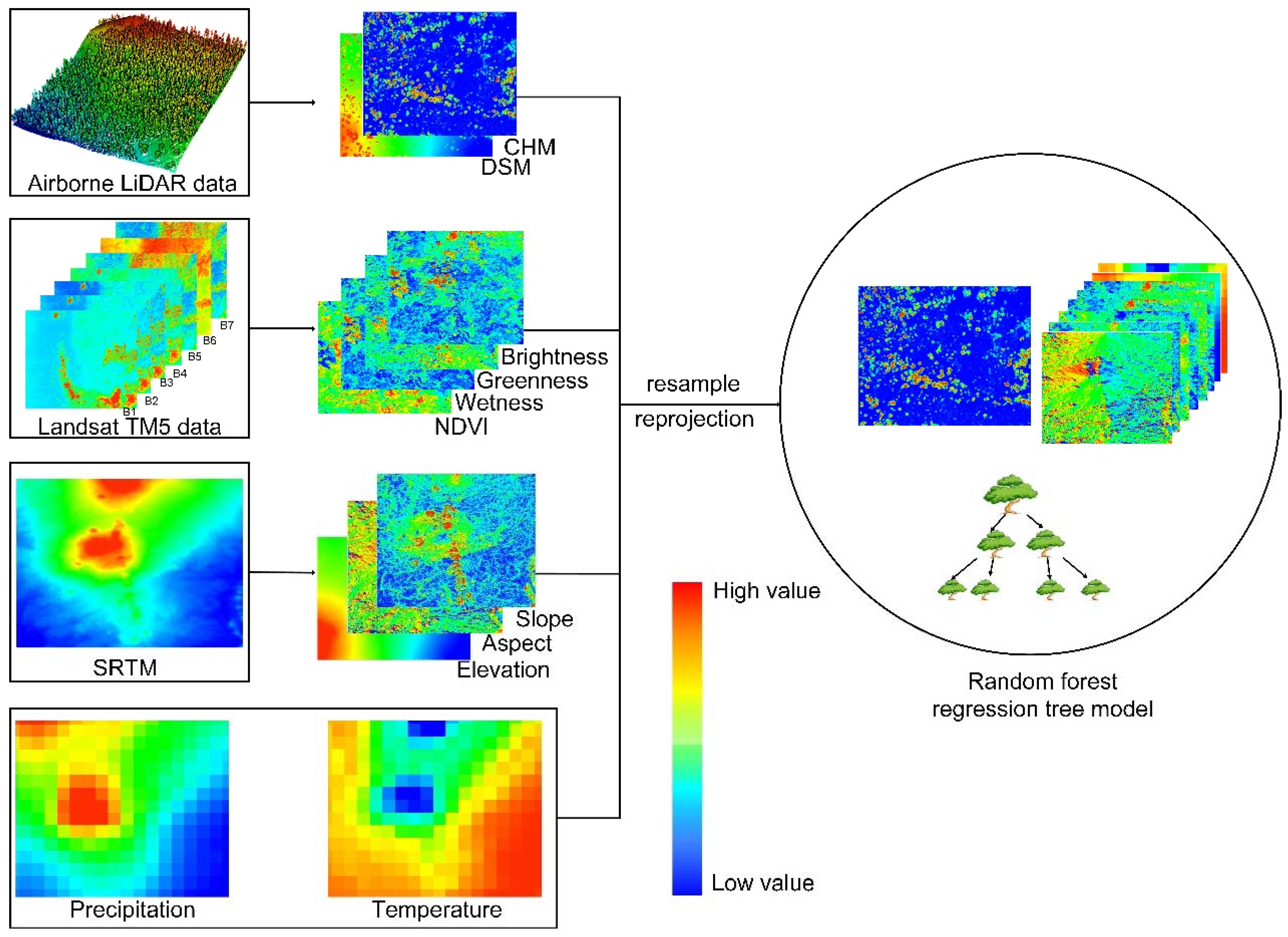
2.3. Ancillary Datasets
3. Methods
3.1. Data Preprocessing
3.1.1. Airborne LiDAR Data
3.1.2. Ancillary Datasets
3.2. Evaluation of RF Transferability on Canopy Height Prediction
3.2.1. The Influence of Locations
3.2.2. The Influence of Vegetation Types
3.2.3. The Influence of Spatial Scales
4. Results
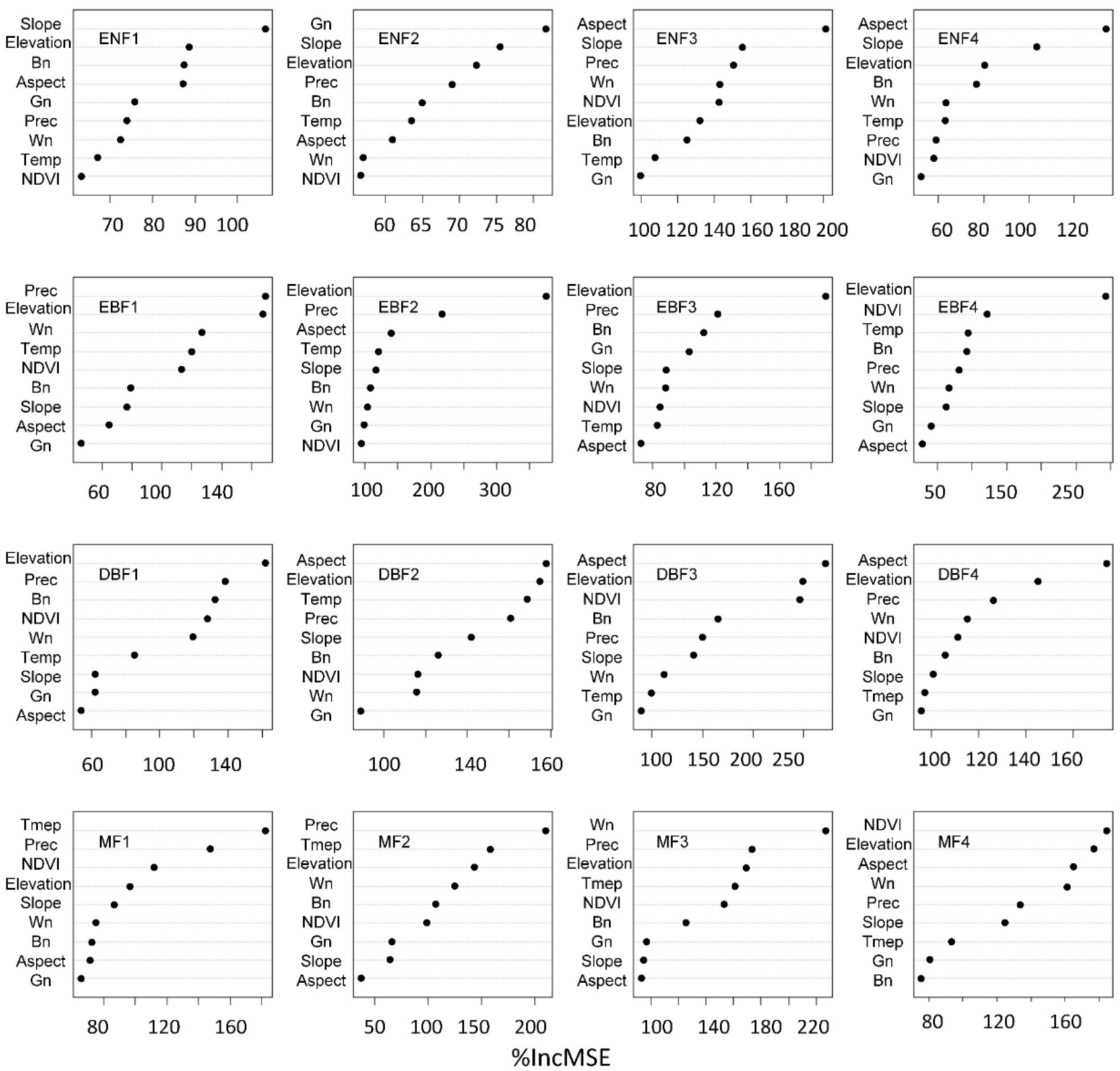
4.1. Variable Importance for RF-Based Canopy Height Prediction
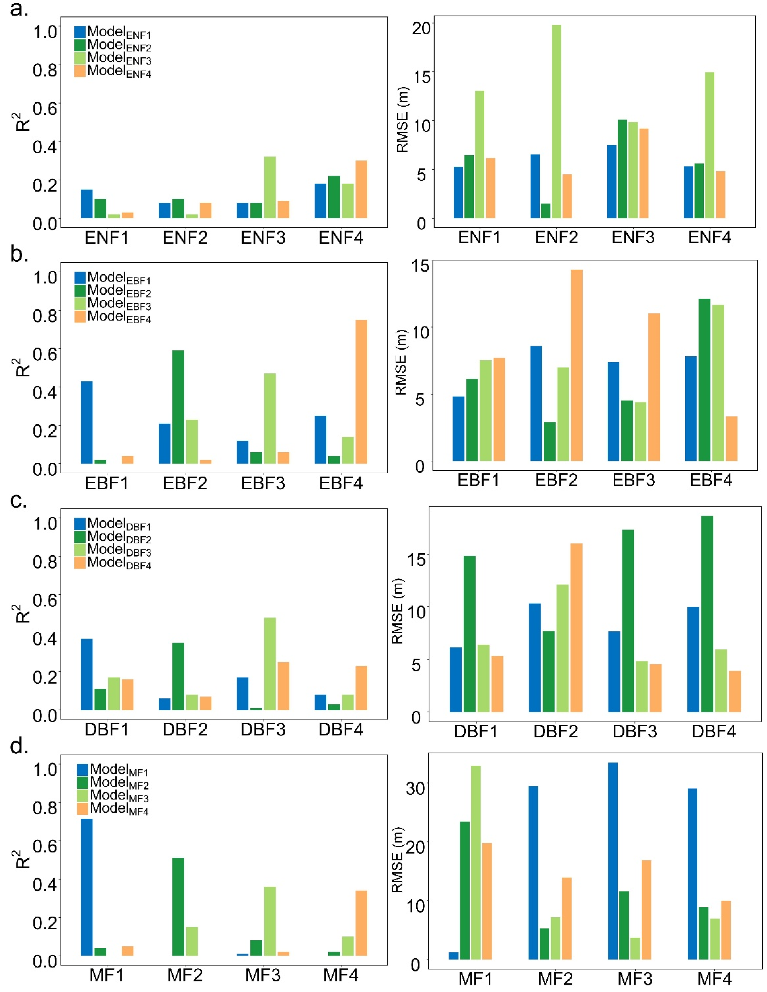
4.2. The Transferability of RF across Different Locations
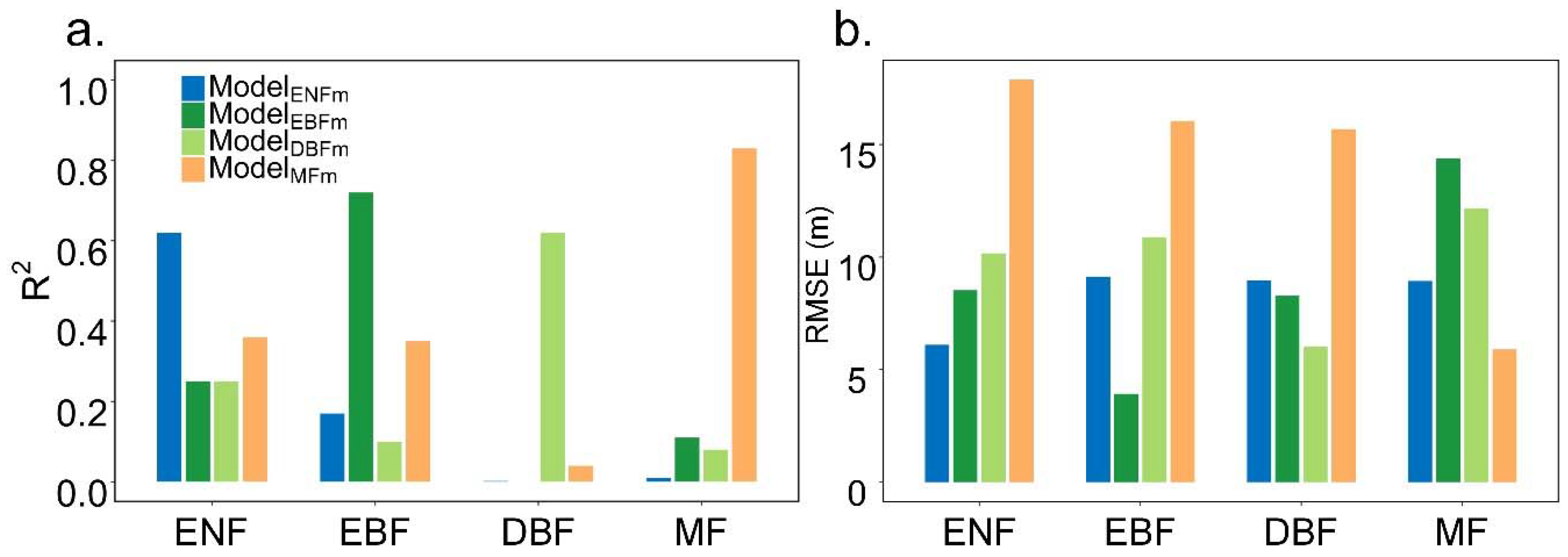
4.3. The Transferability of RF across Different Vegetation Types
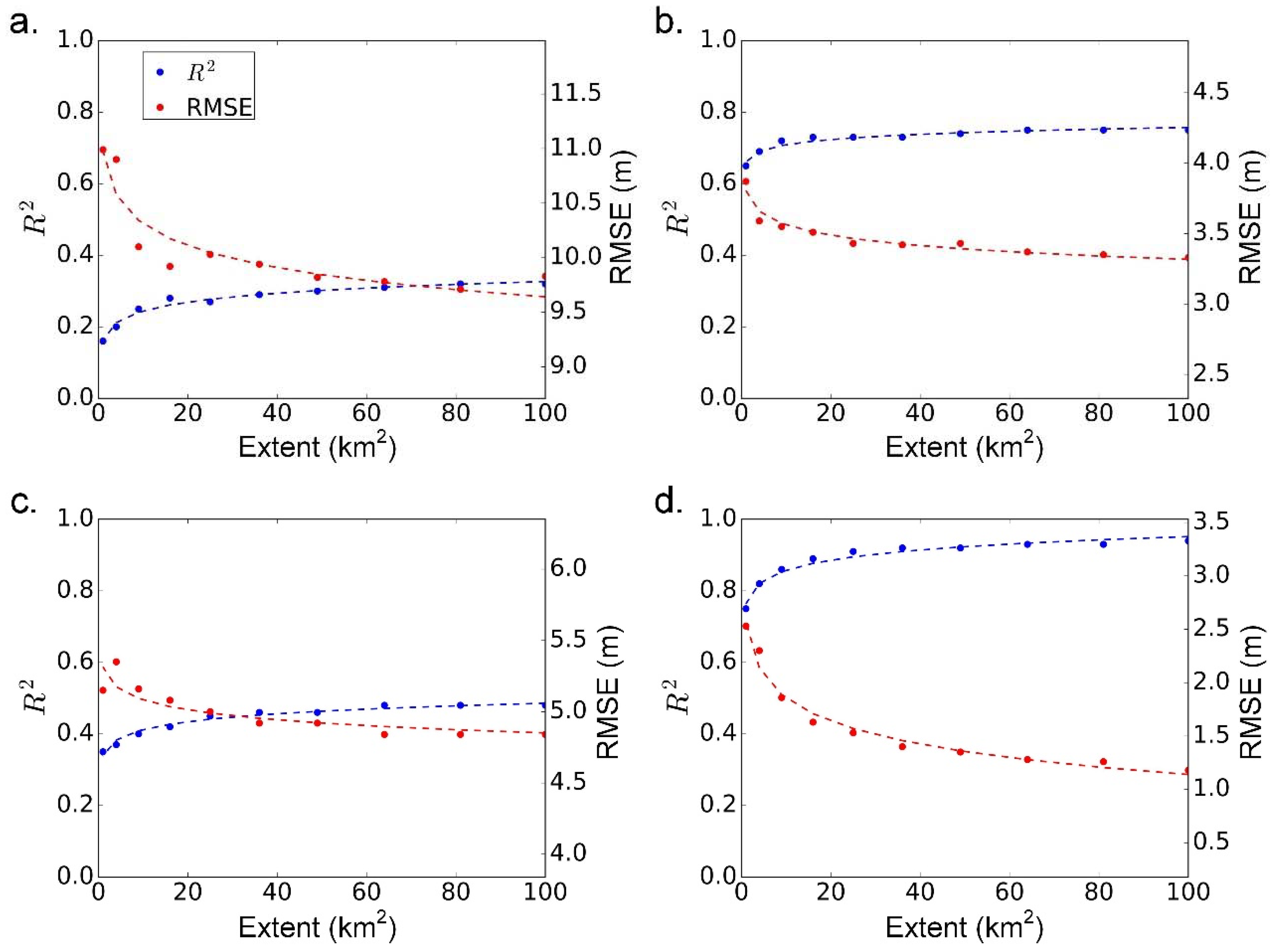
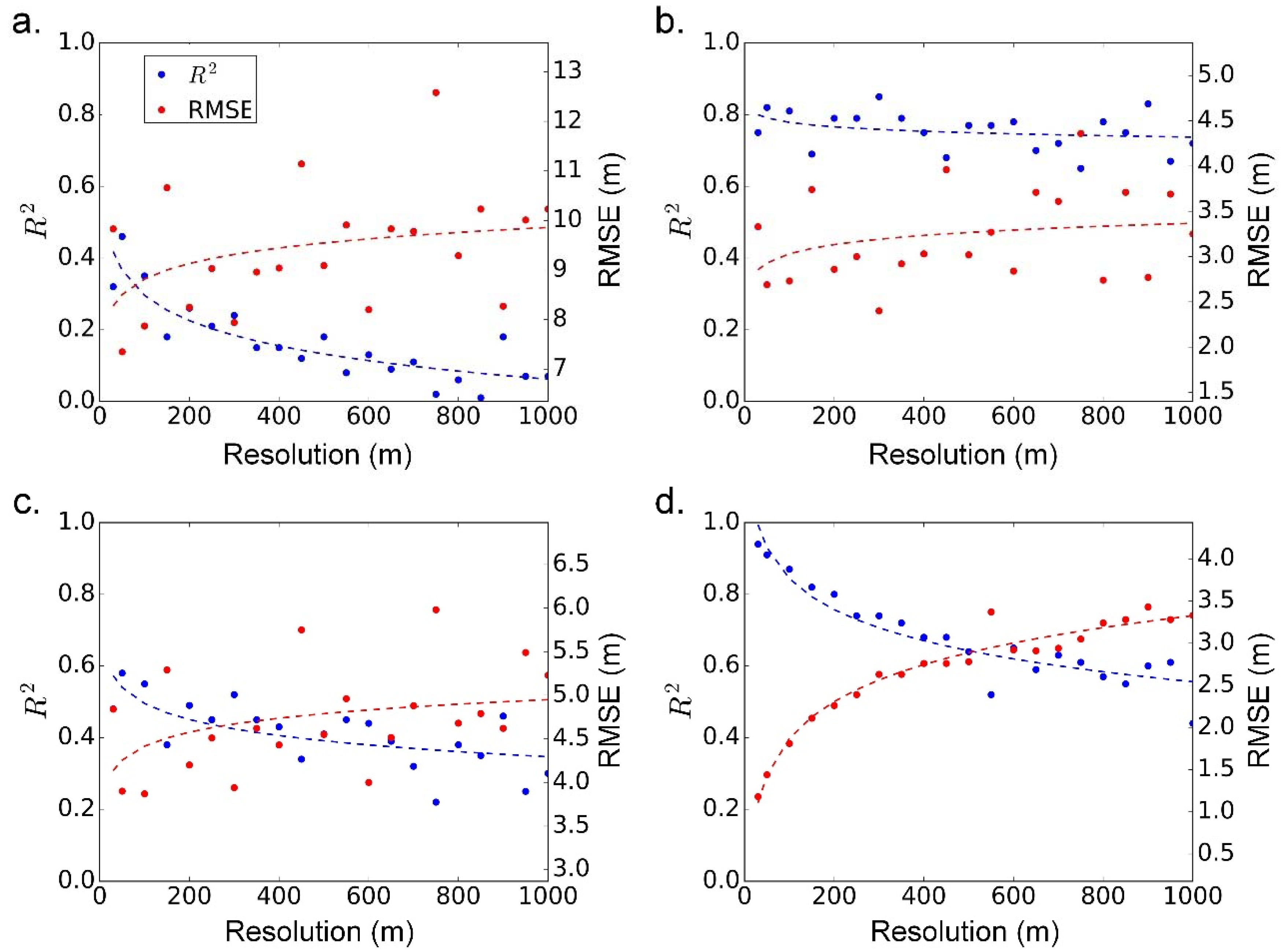
4.4. The Transferability of RF across Different Spatial Scales
5. Discussion
6. Conclusions
Author Contributions
Funding
Acknowledgments
Conflicts of Interest
References
- Costanza, R.; d’Arge, R.; de Groot, R.; Farber, S.; Grasso, M.; Hannon, B.; Limburg, K.; Naeem, S.; O’Neill, R.V.; Paruelo, J.; et al. The value of the world’s ecosystem services and natural capital. Nature 1997, 387, 253–260. [Google Scholar] [CrossRef]
- Houghton, R. Aboveground forest biomass and the global carbon balance. Glob. Chang. Biol. 2005, 11, 945–958. [Google Scholar] [CrossRef]
- Pan, Y.; Birdsey, R.A.; Fang, J.; Houghton, R.; Kauppi, P.E.; Kurz, W.A.; Phillips, O.L.; Shvidenko, A.; Lewis, S.L.; Canadell, J.G. A large and persistent carbon sink in the world’s forests. Science 2011, 333, 988–993. [Google Scholar] [CrossRef] [PubMed]
- Balzter, H.; Rowland, C.S.; Saich, P. Forest canopy height and carbon estimation at monks wood national nature reserve, UK, using dual-wavelength SAR interferometry. Remote Sens. Environ. 2007, 108, 224–239. [Google Scholar] [CrossRef]
- Chave, J.; Andalo, C.; Brown, S.; Cairns, M.; Chambers, J.; Eamus, D.; Fölster, H.; Fromard, F.; Higuchi, N.; Kira, T. Tree allometry and improved estimation of carbon stocks and balance in tropical forests. Oecologia 2005, 145, 87–99. [Google Scholar] [CrossRef] [PubMed]
- Chen, G.; Ozelkan, E.; Singh, K.K.; Zhou, J.; Brown, M.R.; Meentemeyer, R.K. Uncertainties in mapping forest carbon in urban ecosystems. J. Environ. Manag. 2017, 187, 229–238. [Google Scholar] [CrossRef] [PubMed]
- Hu, T.; Su, Y.; Xue, B.; Liu, J.; Zhao, X.; Fang, J.; Guo, Q. Mapping global forest aboveground biomass with spaceborne LiDAR, optical imagery, and forest inventory data. Remote Sens. 2016, 8, 565. [Google Scholar] [CrossRef]
- Xue, B.L.; Guo, Q.; Hu, T.; Xiao, J.; Yang, Y.; Wang, G.; Tao, S.; Su, Y.; Liu, J.; Zhao, X. Global patterns of woody residence time and its influence on model simulation of aboveground biomass. Glob. Biogeochem. Cycles 2017, 31, 821–835. [Google Scholar] [CrossRef]
- Zhang, G.; Ganguly, S.; Nemani, R.R.; White, M.A.; Milesi, C.; Hashimoto, H.; Wang, W.; Saatchi, S.; Yu, Y.; Myneni, R.B. Estimation of forest aboveground biomass in California using canopy height and leaf area index estimated from satellite data. Remote Sens. Environ. 2014, 151, 44–56. [Google Scholar] [CrossRef]
- Prush, V.; Lohman, R. Forest canopy heights in the pacific northwest based on InSAR phase discontinuities across short spatial scales. Remote Sens. 2014, 6, 3210–3226. [Google Scholar] [CrossRef]
- Donoghue, D.; Watt, P. Using LiDAR to compare forest height estimates from IKONOS and Landsat ETM+ data in Sitka spruce plantation forests. Int. J. Remote Sens. 2006, 27, 2161–2175. [Google Scholar] [CrossRef]
- McCombs, J.W.; Roberts, S.D.; Evans, D.L. Influence of fusing LiDAR and multispectral imagery on remotely sensed estimates of stand density and mean tree height in a managed loblolly pine plantation. For. Sci. 2003, 49, 457–466. [Google Scholar]
- Lefsky, M.A.; Keller, M.; Pang, Y.; De Camargo, P.B.; Hunter, M.O. Revised method for forest canopy height estimation from geoscience laser altimeter system waveforms. J. Appl. Remote Sens. 2007, 1, 013537. [Google Scholar] [CrossRef]
- Su, Y.; Ma, Q.; Guo, Q. Fine-resolution forest tree height estimation across the sierra nevada through the integration of spaceborne LiDAR, airborne LiDAR, and optical imagery. Int. J. Digit. Earth 2016, 10, 307–323. [Google Scholar] [CrossRef]
- Lefsky, M.A.; Cohen, W.B.; Parker, G.G.; Harding, D.J. LiDAR remote sensing for ecosystem studies: LiDAR, an emerging remote sensing technology that directly measures the three-dimensional distribution of plant canopies, can accurately estimate vegetation structural attributes and should be of particular interest to forest, landscape, and global ecologists. BioScience 2002, 52, 19–30. [Google Scholar]
- Clark, M.L.; Clark, D.B.; Roberts, D.A. Small-footprint LiDAR estimation of sub-canopy elevation and tree height in a tropical rain forest landscape. Remote Sens. Environ. 2004, 91, 68–89. [Google Scholar] [CrossRef]
- Alexander, C.; Bøcher, P.K.; Arge, L.; Svenning, J.-C. Regional-scale mapping of tree cover, height and main phenological tree types using airborne laser scanning data. Remote Sens. Environ. 2014, 147, 156–172. [Google Scholar] [CrossRef]
- Lefsky, M.A. A global forest canopy height map from the moderate resolution imaging spectroradiometer and the geoscience laser altimeter system. Geophys. Res. Lett. 2010, 37, 78–82. [Google Scholar] [CrossRef]
- Simard, M.; Pinto, N.; Fisher, J.B.; Baccini, A. Mapping forest canopy height globally with spaceborne LiDAR. J. Geophys. Res. Biogeosci. 2011, 116, G04021. [Google Scholar] [CrossRef]
- Hansen, M.C.; Potapov, P.V.; Goetz, S.J.; Turubanova, S.; Tyukavina, A.; Krylov, A.; Kommareddy, A.; Egorov, A. Mapping tree height distributions in sub-saharan africa using Landsat 7 and 8 data. Remote Sens. Environ. 2016, 185, 221–232. [Google Scholar] [CrossRef]
- Wang, Y.; Li, G.; Ding, J.; Guo, Z.; Tang, S.; Wang, C.; Huang, Q.; Liu, R.; Chen, J.M. A combined GLAS and MODIS estimation of the global distribution of mean forest canopy height. Remote Sens. Environ. 2016, 174, 24–43. [Google Scholar] [CrossRef] [Green Version]
- Mountrakis, G.; Im, J.; Ogole, C. Support vector machines in remote sensing: A review. ISPRS J. Photogramm. Remote Sens. 2011, 66, 247–259. [Google Scholar] [CrossRef]
- Chen, G.; Hay, G.J. A support vector regression approach to estimate forest biophysical parameters at the object level using airborne LiDAR transects and quickbird data. Photogramm. Eng. Remote Sens. 2011, 77, 733–741. [Google Scholar] [CrossRef]
- Cutler, M.E.J.; Boyd, D.S.; Foody, G.M.; Vetrivel, A. Estimating tropical forest biomass with a combination of sar image texture and Landsat TM data: An assessment of predictions between regions. ISPRS J. Photogramm. Remote Sens. 2012, 70, 66–77. [Google Scholar] [CrossRef] [Green Version]
- Tetko, I.V.; Livingstone, D.J.; Luik, A.I. Neural network studies. 1. Comparison of overfitting and overtraining. J. Chem. Inf. Comput. Sci. 1995, 35, 826–833. [Google Scholar] [CrossRef]
- Zhu, X.; Liu, D. Improving forest aboveground biomass estimation using seasonal Landsat NDVI time-series. ISPRS J. Photogramm. Remote Sens. 2015, 102, 222–231. [Google Scholar] [CrossRef]
- Cao, L.; Pan, J.; Li, R.; Li, J.; Li, Z. Integrating airborne LiDAR and optical data to estimate forest aboveground biomass in arid and semi-arid regions of China. Remote Sens. 2018, 10, 532. [Google Scholar] [CrossRef]
- Prasad, A.M.; Iverson, L.R.; Liaw, A. Newer classification and regression tree techniques: Bagging and random forests for ecological prediction. Ecosystems 2006, 9, 181–199. [Google Scholar] [CrossRef]
- Breiman, L. Random forests. Mach. Learn. 2001, 45, 5–32. [Google Scholar] [CrossRef]
- Ahmed, O.S.; Franklin, S.E.; Wulder, M.A.; White, J.C. Characterizing stand-level forest canopy cover and height using Landsat time series, samples of airborne LiDAR, and the random forest algorithm. ISPRS J. Photogramm. Remote Sens. 2015, 101, 89–101. [Google Scholar] [CrossRef]
- Su, Y.; Guo, Q.; Xue, B.; Hu, T.; Alvarez, O.; Tao, S.; Fang, J. Spatial distribution of forest aboveground biomass in China: Estimation through combination of spaceborne LiDAR, optical imagery, and forest inventory data. Remote Sens. Environ. 2016, 173, 187–199. [Google Scholar] [CrossRef]
- Keane, R.E.; Parsons, R.A.; Hessburg, P.F. Estimating historical range and variation of landscape patch dynamics: Limitations of the simulation approach. Ecol. Model. 2002, 151, 29–49. [Google Scholar] [CrossRef]
- Hall, R.; Skakun, R.; Arsenault, E.; Case, B. Modeling forest stand structure attributes using Landsat ETM+ data: Application to mapping of aboveground biomass and stand volume. For. Ecol. Manag. 2006, 225, 378–390. [Google Scholar] [CrossRef]
- Turner, M.G.; Dale, V.H.; Gardner, R.H. Predicting across scales: Theory development and testing. Landsc. Ecol. 1989, 3, 245–252. [Google Scholar] [CrossRef]
- Turner, M.G.; O’Neill, R.V.; Gardner, R.H.; Milne, B.T. Effects of changing spatial scale on the analysis of landscape pattern. Landsc. Ecol. 1989, 3, 153–162. [Google Scholar] [CrossRef]
- Masek, J.; Vermote, E.; Saleous, N.; Wolfe, R.; Hall, F.; Huemmrich, F.; Gao, F.; Kutler, J.; Lim, T. LEDAPS Calibration, Reflectance, Atmospheric Correction Preprocessing Code, Version 2; ORNL DAAC: Oak Ridge, TN, USA, 2013.
- Broxton, P.D.; Zeng, X.; Sulla-Menashe, D.; Troch, P.A. A global land cover climatology using MODIS data. J. Appl. Meteorol. Clim. 2014, 53, 1593–1605. [Google Scholar] [CrossRef]
- Mohan, C.; Western, A.W.; Wei, Y.; Saft, M. Predicting groundwater recharge for varying land cover and climate conditions—A global meta-study. Hydrol. Earth Syst. Sci. 2018, 22, 2689–2703. [Google Scholar] [CrossRef]
- Sharma, A.; Goyal, M.K. Assessment of ecosystem resilience to hydroclimatic disturbances in India. Glob. Chang. Biol. 2018, 24, 432–441. [Google Scholar] [CrossRef] [PubMed]
- Zhao, X.; Guo, Q.; Su, Y.; Xue, B. Improved progressive tin densification filtering algorithm for airborne LiDAR data in forested areas. ISPRS J. Photogramm. Remote Sens. 2016, 117, 79–91. [Google Scholar] [CrossRef]
- Guo, Q.H.; Li, W.K.; Yu, H.; Alvarez, O. Effects of topographic variability and LiDAR sampling density on several dem interpolation methods. Photogramm. Eng. Remote Sens. 2010, 76, 701–712. [Google Scholar] [CrossRef]
- Ma, Q.; Su, Y.; Guo, Q. Comparison of canopy cover estimations from airborne LiDAR, aerial imagery, and satellite imagery. IEEE J. Sel. Top. Appl. Earth Obs. Remote Sens. 2017, 10, 4225–4236. [Google Scholar] [CrossRef]
- Jakubowski, M.K.; Guo, Q.; Kelly, M. Tradeoffs between LiDAR pulse density and forest measurement accuracy. Remote Sens. Environ. 2013, 130, 245–253. [Google Scholar] [CrossRef]
- Singh, K.K.; Chen, G.; Vogler, J.B.; Meentemeyer, R.K. When big data are too much: Effects of LiDAR returns and point density on estimation of forest biomass. IEEE J. Sel. Top. Appl. Earth Obs. Remote Sens. 2016, 9, 3210–3218. [Google Scholar] [CrossRef]
- Næsset, E.; Bjerknes, K.-O. Estimating tree heights and number of stems in young forest stands using airborne laser scanner data. Remote Sens. Environ. 2001, 78, 328–340. [Google Scholar] [CrossRef]
- Hwang, S.; Lee, I. Current status of tree height estimation from airborne LiDAR data. Korean J. Remote Sens. 2011, 27, 389–401. [Google Scholar] [CrossRef]
- Van Leeuwen, W.J.; Huete, A.R.; Laing, T.W. MODIS vegetation index compositing approach: A prototype with AVHRR data. Remote Sens. Environ. 1999, 69, 264–280. [Google Scholar] [CrossRef]
- Liaw, A.; Wiener, M. Classification and regression by randomforest. R News 2002, 2, 18–22. [Google Scholar]
- Das, A.J.; Stephenson, N.L.; Flint, A.; Das, T.; Van Mantgem, P.J. Climatic correlates of tree mortality in water-and energy-limited forests. PLoS ONE 2013, 8, 69917–69927. [Google Scholar] [CrossRef] [PubMed]
- Rich, P.M.; Hetrick, W.A.; Saving, S.C. Modeling Topographic Influences on Solar Radiation: A Manual for the Solarflux Model; Los Alamos National Lab.: Los Alamos, NM, USA, 1995.
- Zon, R. Forests and Water in the Light of Scientific Investigation; U.S. Government Printing Office: Statesboro, GA, USA, 1927.
- Kogan, F.; Stark, R.; Gitelson, A.; Jargalsaikhan, L.; Dugrajav, C.; Tsooj, S. Derivation of pasture biomass in mongolia from AVHRR-based vegetation health indices. Int. J. Remote Sens. 2004, 25, 2889–2896. [Google Scholar] [CrossRef]
- Freitas, S.R.; Mello, M.C.S.; Cruz, C.B.M. Relationships between forest structure and vegetation indices in atlantic rainforest. For. Ecol. Manag. 2005, 218, 353–362. [Google Scholar] [CrossRef]
- Linderman, M.A.; An, L.; Bearer, S.; He, G.; Ouyang, Z.; Liu, J. Modeling the spatio-temporal dynamics and interactions of households, landscapes, and giant panda habitat. Ecol. Model. 2005, 183, 47–65. [Google Scholar] [CrossRef]
- Foody, G.M.; Boyd, D.S.; Cutler, M.E. Predictive relations of tropical forest biomass from Landsat TM data and their transferability between regions. Remote Sens. Environ. 2003, 85, 463–474. [Google Scholar] [CrossRef]
- Aarts, G.; Fieberg, J.; Brasseur, S.; Matthiopoulos, J. Quantifying the effect of habitat availability on species distributions. J. Anim. Ecol. 2013, 82, 1135–1145. [Google Scholar] [CrossRef] [PubMed] [Green Version]
- Matthiopoulos, J.; Hebblewhite, M.; Aarts, G.; Fieberg, J. Generalized functional responses for species distributions. Ecology 2011, 92, 583–589. [Google Scholar] [CrossRef] [PubMed] [Green Version]
- Chen, Q.; Laurin, G.V.; Battles, J.J.; Saah, D. Integration of airborne LiDAR and vegetation types derived from aerial photography for mapping aboveground live biomass. Remote Sens. Environ. 2012, 121, 108–117. [Google Scholar] [CrossRef]
- Baldwin, D.J.; Weaver, K.; Schnekenburger, F.; Perera, A.H. Sensitivity of landscape pattern indices to input data characteristics on real landscapes: Implications for their use in natural disturbance emulation. Landsc. Ecol. 2004, 19, 255–271. [Google Scholar] [CrossRef]
- Buyantuyev, A.; Wu, J. Effects of thematic resolution on landscape pattern analysis. Landsc. Ecol. 2007, 22, 7–13. [Google Scholar] [CrossRef]
- Moody, A.; Woodcock, C. Scale-dependent errors in the estimation of land-cover proportions: Implications for global land-cover datasets. Photogramm. Eng. Remote Sens. 1994, 60, 585–594. [Google Scholar]
- Proença, V.; Pereira, H.M.; Vicente, L. Resistance to wildfire and early regeneration in natural broadleaved forest and pine plantation. Acta Oecol. 2010, 36, 626–633. [Google Scholar] [CrossRef]
- Box, G.E.; Draper, N.R. Empirical Model-Building and Response Surfaces; John Wiley & Sons: New York, NY, USA, 1987. [Google Scholar]
- Woodcock, C.E. Uncertainty in Remote Sensing and GIS; John Wiley & Sons, Ltd.: Hoboken, NJ, USA, 2002; pp. 19–24. [Google Scholar]
- Vancoillie, F.; Verbeke, L.; De Wulf, R. Artificial Neural Network Training for Savanna Vegetation Mapping: Transferring Previously Learned Experience to New Learning Tasks; International Workshop on Geo-Spatial Knowledge Processing for Natural Resource Management: Varese, Italy, 2001. [Google Scholar]


| Study Site | Longitude (°) | Latitude (°) | Elevation (m) | Slope (°) | Area (km2) | Percentage * (%) | Mean Tree Height (m) | Mean Canopy Cover | Forest Integrity |
|---|---|---|---|---|---|---|---|---|---|
| ENF1 | −121.68 | 43.89 | 1631.69 | 6.49 | 96.87 | 100.00 | 6.11 | 0.67 | unmanaged |
| ENF2 | −118.51 | 44.54 | 1600.22 | 11.12 | 99.00 | 99.22 | 1.50 | 0.28 | unmanaged |
| ENF3 | −123.75 | 42.69 | 683.47 | 21.07 | 98.00 | 100.00 | 18.77 | 0.89 | unmanaged |
| ENF4 | −114.71 | 46.62 | 1789.64 | 15.56 | 100.00 | 88.95 | 4.23 | 0.38 | unmanaged |
| EBF1 | −84.60 | 30.54 | 51.24 | 3.37 | 90.12 | 75.84 | 13.54 | 0.86 | unmanaged |
| EBF2 | −85.34 | 30.38 | 28.81 | 1.99 | 100.93 | 89.58 | 16.36 | 0.95 | unmanaged |
| EBF3 | −88.97 | 30.88 | 39.16 | 2.50 | 95.66 | 72.75 | 15.78 | 0.86 | unknown |
| EBF4 | −82.43 | 30.25 | 45.36 | 2.44 | 100.00 | 99.52 | 6.77 | 0.57 | unknown |
| DBF1 | −76.54 | 38.53 | 47.38 | 5.02 | 100.00 | 80.70 | 13.46 | 0.62 | unmanaged |
| DBF2 | −86.92 | 36.25 | 217.52 | 11.08 | 100.00 | 100.00 | 26.09 | 0.91 | unmanaged |
| DBF3 | −86.29 | 39.13 | 593.27 | 17.69 | 98.27 | 100.00 | 10.86 | 0.82 | unmanaged |
| DBF4 | −84.46 | 36.21 | 242.08 | 8.36 | 100.00 | 100.00 | 10.08 | 0.91 | unknown |
| MF1 | −91.77 | 33.02 | 47.64 | 2.55 | 99.00 | 96.35 | 38.78 | 0.95 | managed |
| MF2 | −80.78 | 33.79 | 52.61 | 3.17 | 101.00 | 100.00 | 16.68 | 0.74 | unmanaged |
| MF3 | −69.51 | 43.93 | 37.69 | 4.05 | 100.00 | 91.77 | 7.21 | 0.73 | unknown |
| MF4 | −123.81 | 45.16 | 364.89 | 15.95 | 100.00 | 67.58 | 19.78 | 0.89 | unmanaged |
| Study Area | Year | Month | Accuracy (m) | Ground Density (pts/m2) | Flight Height (m) | Sensor Type | Pulse Rate (kHz) | Scan Rate (Hz) | Data Source |
|---|---|---|---|---|---|---|---|---|---|
| ENF1 | 2009–2010 | Jan, Feb, Mar, Apr, Sep, Oct | 0.05 | 3.20 | 900–1300 | LeicaALS50II, ALS60 | 105.00 | 52.00 | Oregon Department of Geology and Mineral Industries |
| ENF2 | 2008 | Aug | 0.05 | 8.00 | 900 | LeicaALS50II | 105.00 | 52.20 | Oregon Department of Geology and Mineral Industries |
| ENF3 | 2012 | Aug | 0.05 | 8.00 | 900–1300 | LeicaALS50, ALS60, ALS70 | 52.2@900 m, 46.7@1300 m | NA | Oregon Department of Geology and Mineral Industries |
| ENF4 | 2011 | Aug | 0.04 | 4.00 | 1200 | LeicaALS60 | 88.00 | NA | United States Geological Survey |
| EBF1 | 2007–2008 | Mar | 0.08 | 1.42 | 2286 | LeicaALS50 | 52.50 | 24.00 | Northwest Florida Water Management district |
| EBF2 | 2007 | Feb, Mar | 0.01 | 2.73 | 800 | LeicaALS50 | 55.00 | 36.00 | Northwest Florida Water Management district |
| EBF3 | 2006 | Mar, Apr | 0.18 | 0.33 | 2438 | LeicaALS50 | 38.00 | 20.00 | Mississippi department of environment quality |
| EBF4 | 2010 | Mar, Apr | 0.12 | 1.00 | 1371 | RieglLMS-Q680, LMS-Q680i | 100.00 | NA | United States Geological Survey |
| DBF1 | 2011 | Mar | 0.10 | 1.22 | 2174 | Leica ALS50II | 96.80 | 39.80 | Maryland Department of Information Technology |
| DBF2 | 2011 | Mar | 0.18 | 1.45 | 1524 | Optech3100 | 70.00 | 35.00 | United States Geological Survey |
| DBF3 | 2011 | Apr | 0.13 | 1.30 | 1981 | LeicaALS50II, ALS60 OptechALTM Gemini | 115.60 | 41.80 | United States Geological Survey |
| DBF4 | 2011 | Mar, Apr | 0.06 | 2.77 | 1981 | Leica ALS50II | 115.60 | 46.80 | United States Geological Survey |
| MF1 | 2011–2012 | Jul | 0.23 | 2.00 | 2286 | OptechALTM213 | 50.00 | 26.00 | United States Geological Survey |
| MF2 | 2010 | Mar | 0.23 | 2.37 | NA | NA | NA | NA | United States Geological Survey |
| MF3 | 2010 | Sep | 0.15 | 2.40 | NA | NA | NA | NA | United States Geological Survey |
| MF4 | 2010 | Apr | 0.04 | 8.00 | 900–1300 | LeicaALS50,ALS60 | 105.00 | 52.00 | Department of Geology and Mineral Industries |
| Variable | Year | Resolution (m) | Data Source |
|---|---|---|---|
| Land cover map | 2001–2010 | 500 | MODIS |
| Landsat TM images | 2006–2012 | 30 | Land surface reflectance product |
| NDVI | 2006–2012 | 30 | Land surface reflectance product |
| Brightness calculated from Landsat TM images | 2006–2012 | 30 | Land surface reflectance product |
| Greenness calculated from Landsat TM images | 2006–2012 | 30 | Land surface reflectance product |
| Wetness calculated from Landsat TM images | 2006–2012 | 30 | Land surface reflectance product |
| Elevation | 2000 | 30 | SRTM |
| Slope | 2000 | 30 | SRTM |
| Aspect | 2000 | 30 | SRTM |
| Annual mean temperature | 1981–2010 | 800 | PRISM |
| Annual mean precipitation | 1981–2010 | 800 | PRISM |
| Site 1 | Site 2 | Site 3 | Site 4 | |||||
|---|---|---|---|---|---|---|---|---|
| R2 | RMSE (m) | R2 | RMSE (m) | R2 | RMSE (m) | R2 | RMSE (m) | |
| ENF | 0.15 | 5.26 | 0.10 | 1.48 | 0.32 | 9.83 | 0.30 | 4.82 |
| EBF | 0.43 | 4.83 | 0.59 | 2.91 | 0.47 | 4.40 | 0.75 | 8.78 |
| DBF | 0.37 | 6.15 | 0.35 | 7.68 | 0.48 | 4.84 | 0.23 | 3.91 |
| MF | 0.94 | 1.18 | 0.51 | 5.26 | 0.36 | 3.72 | 0.34 | 9.96 |
| Site 1 | Site 2 | Site 3 | Site 4 | |||||
|---|---|---|---|---|---|---|---|---|
| ΔR2 | ΔRMSE (m) | ΔR2 | ΔRMSE (m) | ΔR2 | ΔRMSE (m) | ΔR2 | ΔRMSE (m) | |
| ENF | 0.12 | −0.72 | 0.11 | −0.10 | 0.07 | −0.60 | 0.07 | −1.26 |
| EBF | 0.08 | −0.29 | 0.02 | −0.03 | 0.06 | −0.22 | 0.03 | −0.24 |
| DBF | 0.07 | −0.33 | 0.01 | −0.07 | 0.06 | −0.29 | 0.10 | −0.25 |
| MF | −0.03 | 0.30 | 0.05 | −0.25 | 0.08 | −0.15 | 0.01 | −0.14 |
| ModelTnv | ModelTv | |||
|---|---|---|---|---|
| ΔR2 | ΔRMSE (m) | ΔR2 | ΔRMSE (m) | |
| ENF | −0.01 | 0.08 | −0.01 | 0.06 |
| EBF | −0.02 | 0.15 | −0.02 | 0.16 |
| DBF | −0.01 | 0.11 | −0.01 | 0.08 |
| MF | −0.01 | 0.11 | −0.01 | 0.10 |
© 2018 by the authors. Licensee MDPI, Basel, Switzerland. This article is an open access article distributed under the terms and conditions of the Creative Commons Attribution (CC BY) license (http://creativecommons.org/licenses/by/4.0/).
Share and Cite
Jin, S.; Su, Y.; Gao, S.; Hu, T.; Liu, J.; Guo, Q. The Transferability of Random Forest in Canopy Height Estimation from Multi-Source Remote Sensing Data. Remote Sens. 2018, 10, 1183. https://doi.org/10.3390/rs10081183
Jin S, Su Y, Gao S, Hu T, Liu J, Guo Q. The Transferability of Random Forest in Canopy Height Estimation from Multi-Source Remote Sensing Data. Remote Sensing. 2018; 10(8):1183. https://doi.org/10.3390/rs10081183
Chicago/Turabian StyleJin, Shichao, Yanjun Su, Shang Gao, Tianyu Hu, Jin Liu, and Qinghua Guo. 2018. "The Transferability of Random Forest in Canopy Height Estimation from Multi-Source Remote Sensing Data" Remote Sensing 10, no. 8: 1183. https://doi.org/10.3390/rs10081183
APA StyleJin, S., Su, Y., Gao, S., Hu, T., Liu, J., & Guo, Q. (2018). The Transferability of Random Forest in Canopy Height Estimation from Multi-Source Remote Sensing Data. Remote Sensing, 10(8), 1183. https://doi.org/10.3390/rs10081183