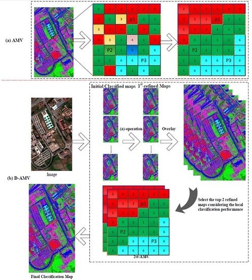
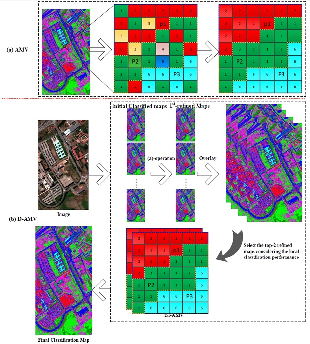
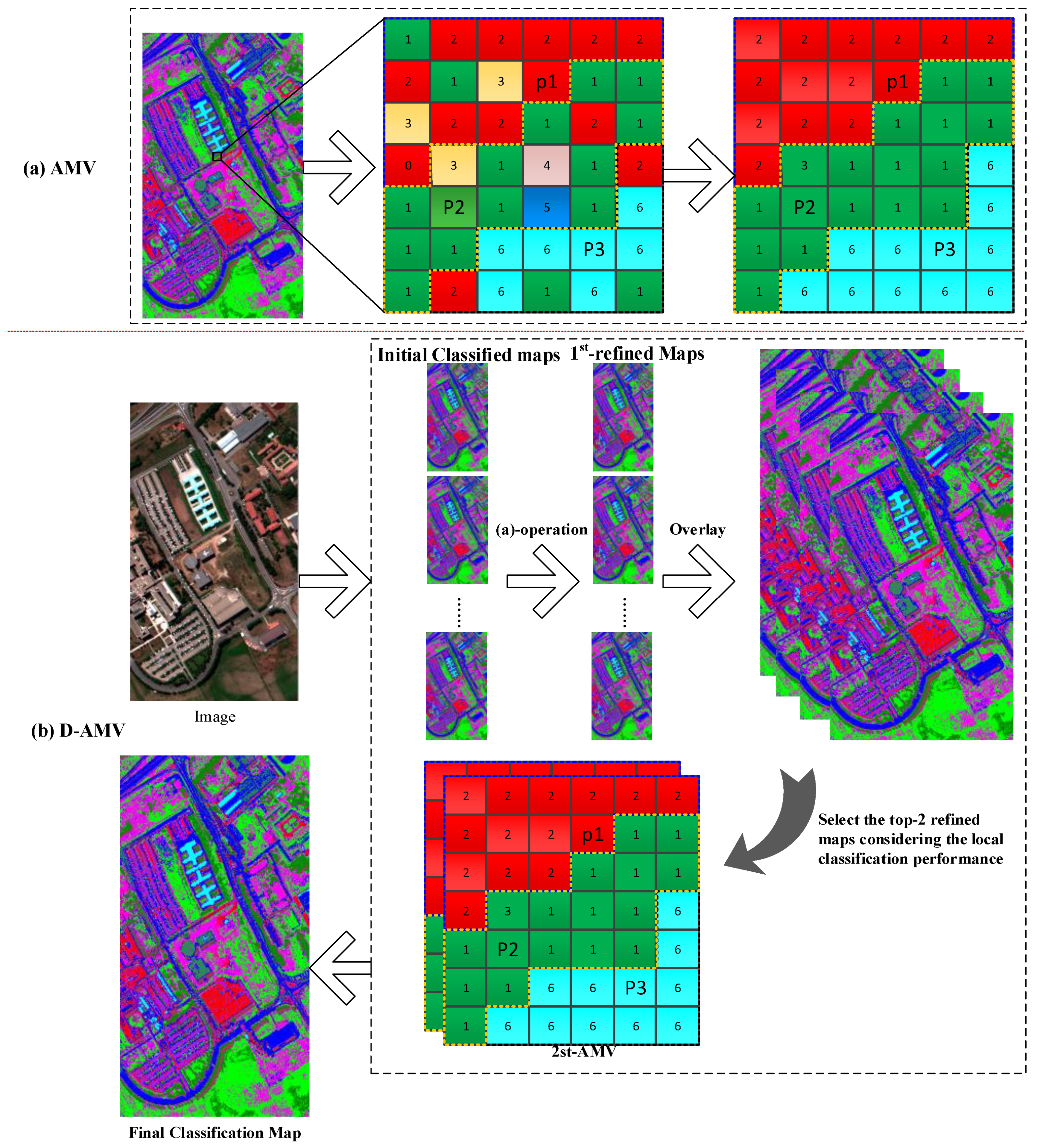
Article

Refining Land Cover Classification Maps Based on Dual-Adaptive Majority Voting Strategy for Very High Resolution Remote Sensing Images

1
Key Laboratory of Subsurface Hydrology and Ecological Effects in Arid Region, Ministry of Education, School of Environmental Science and Engineering, Chang’an University, Xi’an 710054, China
2
The First Topographic Surveying Brigade of Shaanxi Bureau of Surveying and Mapping, Xi’an 710054, China
3
School of Computer Science and Engineering, Xi’an University of Technology, Xi’an 710048, China
4
Faculty of Electrical and Computer Engineering, University of Iceland, IS 107 Reykjavik, Iceland
*
Authors to whom correspondence should be addressed.
Remote Sens. 2018, 10(8), 1238; https://doi.org/10.3390/rs10081238
Submission received: 6 July 2018 / Revised: 30 July 2018 / Accepted: 1 August 2018 / Published: 7 August 2018
(This article belongs to the Section Remote Sensing Image Processing)

Abstract

:
Land cover classification that uses very high resolution (VHR) remote sensing images is a topic of considerable interest. Although many classification methods have been developed, the accuracy and usability of classification systems can still be improved. In this paper, a novel post-processing approach based on a dual-adaptive majority voting strategy (D-AMVS) is proposed to improve the performance of initial classification maps. D-AMVS defines a strategy for refining each label of a classified map that is obtained by different classification methods from the same original image, and fusing the different refined classification maps to generate a final classification result. The proposed D-AMVS contains three main blocks. (1) An adaptive region is generated by gradually extending the region around a central pixel based on two predefined parameters (T1 and T2) to utilize the spatial feature of ground targets in a VHR image. (2) For each classified map, the label of the central pixel is refined according to the majority voting rule within the adaptive region. This is defined as adaptive majority voting. Each initial classified map is refined in this manner pixel by pixel. (3) Finally, the refined classified maps are used to generate a final classification map, and the label of the central pixel in the final classification map is determined by applying AMV again. Each entire classified map is scanned and refined pixel by pixel based on the proposed D-AMVS. The accuracies of the proposed D-AMVS approach are investigated with two remote sensing images with high spatial resolutions of 1.0 m and 1.3 m. Compared with the classical majority voting method and a relatively new post-processing method called the general post-classification framework, the proposed D-AMVS can achieve a land cover classification map with less noise and higher classification accuracies.

Graphical Abstract

1. Introduction

Land cover classification based on remote sensing images plays an important role in providing information regarding the Earth’s surface [1,2,3,4]. For many applications, such as urban vegetation mapping [5], aboveground biomass estimation in forests [6], urban flood mapping [7], and land-use analysis [8], underlying land cover information from remote sensing images is necessary. Very high resolution (VHR) remote sensing images are conveniently available and highly popular in land cover classification. However, substantial research has demonstrated that salt-and-pepper noise is a common phenomenon in the classification of VHR remote sensing images [9,10,11,12,13,14,15,16,17,18].
Several methods have been developed to address this problem. For example, Lv et al. [19] promoted a general post-classification framework for improving land cover classification, and Huang et al. [20] proposed a support vector machine (SVM) ensemble approach for combining different features to improve the classification accuracies of VHR images. In the current study, methods are grouped into two mainstream techniques. The first relatively popular technique is the spatial–spectral feature-based classification method [14,21,22] where the spatial feature is usually extracted to complement insufficient spectral information. For example, the pixel shape index (PSI) has been used to improve VHR image classification [23]. Zhang et al. extended PSI from a “pixel” to an “object” (a group of pixels that are spatial continuously and have high spectral similarity), and proposed an object-based spatial feature called the object correlative index. Various mathematical morphological methods have also been developed to describe structural features and complement spectral features to improve classification accuracy [22,24,25,26,27]. Moreover, spatial filtering is an effective means of reducing noise and extracting spatial features. Kang et al. proposed a method based on an edge-preserving filter and image fusion to enhance classification accuracy [28]. Jia et al. developed an edge-preserving filtering method for improving the performance of VHR image classification [29]. Other methods, such as semantic features [20,30], Markov modeling of spatial features [13], object-based feature extraction [9], and active learning algorithms [31,32], are commonly adopted to complement spectral information for land cover classification. However, despite the numerous features and techniques promoting VHR image classification, not one method can be labeled as “the best” or “the most appropriate one” for all cases, because the classification accuracies of most methods are usually dependent [33,34]. The design and use of feature extraction methods are also dependent on the case at hand. Therefore, the classification accuracy and usability of the VHR image classification method have room for further improvement.
The second technique in this study is post-classification. It defines a post-processing strategy that is often applied to a classified map to remove noise and increase classification accuracy [35,36,37]. Several post-classification methods have been proposed. For example, Lu et al. introduced a structural similarity-based label smoothing approach for refining land cover classification maps [16]. Huang et al. presented a building extraction post-processing framework for VHR imagery. Lv et al. developed a general post-classification framework (GPCF) for improving land cover mapping by using VHR images [19]. Tang et al. and Huang et al. summarized post-processing reclassification approaches systematically in their research [35,38]. Their studies showed that the “sliding window” technique is usually adopted to consider neighboring information for refining the label of the central pixel, wherein the accuracies of the initial classified maps can be improved. Given that everything is related to everything else, and things that are close are more related than things that are more distant according to Tobler’s first law of geography [39,40], pixels with greater proximity are more likely to belong to the same class in terms of a classification problem by using remote sensing images. However, one limitation in considering contextual information through a regular window is that a regular window shape may not cover the different shapes of ground objects in a particular class (i.e., different shapes of buildings, varying shapes of lakes or meadows, etc.). Therefore, the adaptive capability of considering contextual information in post-classification is of great interest.
In this study, we extend our previous research on GPCF [19] and propose an approach called dual-adaptive majority voting strategy (D-AMVS). The extension of this study differs from GPCF in two aspects. First, in the process of refining the label of an initial classified map, neighboring information is considered in an adaptive manner through an adaptive irregular region. Second, when different classified maps are fused, an optimal selection strategy is proposed to dynamically select the classified maps according to their local performance in classification. The initial classified maps are refined based on the adaptive region coupled with the majority voting method. Then, the refined classified maps are used as a candidate set, where the label of each pixel in the final refined classification is determined by the top two refined classified maps, i.e., the maps that present the best performance within the local adaptive region. To demonstrate the effectiveness of this extension, the initial classified maps are obtained by different classifiers or spectral–spatial approaches. The proposed D-AMVS is compared with the existing GPCF and the traditional majority voting approach. Further details are presented in the following sections.

2. D-AMVS Approach for Refining Initial Classification Maps

The proposed D-AMVS aims to utilize spatial information in an adaptive manner and fuse multi-source classified maps to reduce the noise of classification maps. Figure 1b shows the main steps of the proposed strategy. First, multi-source initial classified maps are acquired by different approaches, such as classifiers or spatial–spectral feature-based approaches. Second, the progress of adaptive majority voting (AMV) is defined in Figure 1a, where AMV is used to refine the initial classified maps. The label of each initial classified map of the pixel is refined with an adaptive region generated by gradually extending the region around a central pixel in the sourcing image. Third, in an adaptive region, the local classification performance of each refined classification map is compared with that of others. The top two refined maps are selected, and the label of the central pixel of the adaptive region is assigned by using the class that appears most frequently. Additional details are presented in the following paragraphs.
The construction of the adaptive region surrounding a pixel is pivotal for the proposed D-AMVS. This study employs an adaptive region around a central pixel that has been proposed in the literature [41]. The shape of an adaptive region represents the contextual features surrounding a central pixel, and the size of the adaptive region is constrained by two predefined thresholds (T1 and T2) in spectral and spatial domains. From the investigation in [41], we find that the proposed adaptive region has an advantage in considering contextual information in an adaptive spatial domain (see [42] for more details). Three examples are given in Figure 2 to show the shape-adaptive capability of the proposed region extension method.
In this study, the adaptive region coupled with majority voting is used to refine the multi-source initial classification maps. The refined maps are then fused to generate a final classification result. An initial multi-source classification map is represented by the set I = { I 1 , I 2 , I 3 , , I N } , where N is the total number of initial classified maps. The total number of a specific class ( C l ) within an adaptive region ( R i j ) can be calculated by Equation (1):
S l = p x I k ( C l ) ,   x R i j ,
where S l is the total number of pixels belonging to the specific class C l within the adaptive region R i j . R i j is the extended region around the pixel (i,j) in the spatial domain, and p x I k ( C l ) is labeled as C l in the initial classified map I k . In this context, the label of central pixel xij can be determined by Equation (2):
C ( x i j ) = argmax { s 1 , s 2 , s 3 , s m } ,
where m is the total number of classes for the entire initial classification map, Sm is assumed to be the total number of pixels that are assigned to the m-th class of the initial classification maps for adaptive region R i j , and C ( x i j ) is the label of the central pixel. Therefore, the label of the central pixel ( x i j ) is refined according to the class label that has the maximum performance in the set { s 1 , s 2 , s 3 , s M }.
An initial classified image can be refined pixel by pixel through the corresponding adaptive region. An example is shown in Figure 1a, where P1, P2, and P3 are the three central pixels, and the dotted line with different colors present the different adaptive regions around them. This refining process is defined as AMV. Compared with the regular window-based majority voting approach, the proposed AMV technique can smoothen the noise of the classification map and preserve the shape of different targets.
To further improve classification accuracy and generate the final classification map, inspired by a previous GPCF [19], the refined classification maps are used as candidates to obtain the final classification map. First, the number of classes within an adaptive region ( R i j ) is counted and assigned as N c I k ( R i j ) , where I k is the k-th refined classified map. Therefore, the number of classes within an adaptive region can be calculated for each refined map, where the set is assigned as N c = { N c I 1 ( R i j ) , N c I 2 ( R i j ) , N c I 3 ( R i j ) , , N c I k ( R i j ) } . Second, the set ( N c ) is sorted in a descending order. Then, the top two refined classified maps are used as the selected maps for the following process. The top two refined classified maps are assigned as I a and I b . In theory, because the adaptive region has relatively greater homogeneity in the spectral domain, the pixels within the adaptive region are usually viewed as one target class. Therefore, having fewer classes within an adaptive region means better classification performance for the local region of a refined map. Finally, the number of pixels in each class from the selected refined classified maps I a and I b is considered. The label of the central pixel (i,j) of adaptive region R i j is refined dually by using the class that appears most frequently in the region. In this context, each pixel of an image is taken once as a central pixel to extend the corresponding adaptive region, and the adaptive region is coupled with the majority voting strategy to select the refined maps and determine the label of each pixel in the final classification map.
The difference between the proposed D-AMVS and the previous GPCF [19] lies in two aspects. First, the GPCF directly fuses a set of multi-source initially classified maps to generate the final classification map. By contrast, in the proposed D-AMVS, each initially classified map is refined pixel by pixel to reduce noise. Then, the top two refined maps are selected each time to determine the label of each pixel in the final classification map according to the local classification performance within an adaptive region. In selecting the refined maps, considering the local classification performance within an adaptive region is beneficial to determining the label for a pixel in the final classification map. Second, GPCF determines the label of a pixel in the final classification map by using a regular window and the majority voting technique. On the one hand, because the number of each class within a regular window is affected by the shape of a target when the central pixel of a window is located at the boundary between different classes, determining the label of the central pixel may have a limitation in discrimination. On the other hand, the proposed D-AMVS has an advantage in spatial adaptive capability, wherein the majority voting strategy is applied in an adaptive region that can be adaptive with the shape of a target.

3. Experiment

In this section, two experiments are performed to test the effectiveness of the proposed D-AMVS approach. First, two images with very high spatial resolutions are described in detail. Second, the experimental design and setting of parameters are presented. Lastly, the visual performance and quantitative evaluation are shown for comparison.

3.1. Data Set Description

Two data sets are used in the experiments. The first data set was obtained by the Reflective Optics System Imaging Spectrometer (ROSIS-03) sensor on 8 July 2002 [14,42], and the raw data represent the hyperspectral image of a Pavia University scene with 103 bands and 1.0 m/pixel spatial resolution. The location of this data is near Pavia University, which is located north of the city Pavia in Italy. The original data set is 610 × 340 pixels. For the first experiment, Figure 3a shows a false color image composed of channel numbers 10, 27, and 46 for red, green, and blue, respectively. The ground reference is shown in Figure 3b. Nine information classes are considered in the experiment, as shown in the legend.
The second data set is also a ROSIS-03 image from Pavia Center, Italy. The original size of the image is 1096 × 1096 pixels with a 1.3 m/pixel spatial resolution. However, a 381 pixel-wide strip is removed because of noise, resulting in a “two-part” 1096 × 715 pixel image (Figure 4a). The original image contains 115 bands with a spectral range of 0.43–0.86 μ m . In Figure 4a, three bands, numbered 60, 27, and 17 are selected to compose a false color image in red, green, and blue, respectively. Figure 4b illustrates the ground reference and the nine information classes.

3.2. Experimental Setup and Parameter Setting

In the first experiment, the Pavia University image is adopted to test the effectiveness of the proposed D-AMVS on the basis of the different initial classification maps acquired by the different supervised classifiers. A false color image is used as the input data for land cover classification because the focus of our study is on VHR remote sensing images. Four classical supervised classifiers are embedded in business ENVI4.8. Specifically, neural net (NN), maximum likelihood classification (MLC), Mahalanobis distance (MD), and support vector machine (SVM) are used to obtain the initial classified maps. The software provides the default parameters of each classifier for the Pavia University image. The details of the training samples and testing pixels are given in Table 1.
In the second experiment, the proposed D-AMVS is compared with the traditional majority voting approach and the existing GPCF post-classification approach on the basis of initial classified maps that were obtained by a different spatial–spectral feature approach. A false color image of the Pavia Center scene is adopted for comparison to obtain spatial features. Table 2 shows the number of training and test samples. The parameters of the four spectral–spatial approaches were set based on the above to obtain the initial classified maps.
(1)
Extended morphological profiles (EMPs) [26] are built based on a “disk” structuring element (SE), and the sizes of SE are equal to 2, 4, 6, and 8 in this experiment.
(2)
Multi-shape EMPs (M-EMPs) [25] involve the SE set to shapes equaling “disk, square, diamond, and line,” and the size of each SE is equal to 8.
(3)
The parameters of a recursive filter (RF) [28] are set as follows: δ s = 200 , δ r = 45.0 , and the number of iterations is 3. δ s and δ r denote the spatial and range parameters, respectively. Further details on δ s and δ r can be obtained in literature [28].
(4)
Rolling guidance filter (RGF) [43] is applied to the Pavia Center image with the following parameters: δ s = 200 , δ r = 45.0 , iteration = 3. In RGF, δ s and δ r control the spatial range and spatial weights, respectively.
Apart from these parameter settings for acquiring the initial classified maps in each experiment, majority voting and existing GPCF post-classification approaches are applied with a window size from 3 × 3 to 9 × 9 , as shown in Tables 4 and 6.
To ensure fairness in comparison, the following rules are obeyed in the experiments. First, the parameters of each approach are acquired through a trial-and-error method. Second, SVM with an RBF kernel and threefold cross-validation is used as the supervised classifier to classify the different spatial–spectral features in the second experiment. Third, the initial classified map with the highest accuracies is selected for post-processing based on majority voting and compared with GPCF and the proposed D-AMVS.

3.3. Results and Quantitative Evaluation

The experimental results and comparisons in terms of overall accuracy (OA), Kappa coefficient (Ka), and average accuracies (AA) are detailed below.
Table 3 shows the four initial classified maps acquired by the four supervised classifiers for the Pavia University image. MLC achieves the best accuracy in this test. Therefore, the result of MLC is used for post-classification by adopting the majority voting approach with a different window size (Table 4). Compared with the initial and post-classification maps (Table 3 and Table 4), each of the algorithms, including majority voting, GPCF, and the proposed D-AVMS, can improve classification accuracies. Furthermore, the accuracies of the proposed D-AMVS are more competitive in terms of OA, AA, and Ka. The visual performance comparisons in Figure 5 further verify this experimental conclusion. Compared with the initial classified maps obtained by the MLC classifier, considerable noise can be reduced by the post-processing methods, namely, MV, GPCF, and the proposed D-AMVS. The user accuracy of each class for the different methods is detailed in Table 5, which shows that the user accuracy of most classes can be improved by the proposed D-AMVS approach.
To further demonstrate the advantage of the proposed D-AMVS, Figure 6 shows a zoomed in observation of the comparisons. The observation of the painted metal sheet is represented by a dashed rectangle. The results show the following. First, the shape of the ground target is best preserved in the initial classification map, but much salt-and-pepper noise is observed. Second, although traditional majority voting and GPCF can remove performance noise, the shape of the ground object cannot be maintained. This situation can be attributed to the regular window, which has a limitation in considering spatial contextual information, while the shape of the ground target and the window are inconsistent. Compared with majority voting and GPCF, the proposed D-AMVS has the best classification performance and maintains the preferred shape of the ground target. Additional observations can be obtained from the dashed ellipse region of Figure 6.
To further investigate the effectiveness and confirm the robustness of the proposed D-AMVS approach, the method is applied to an initial classification map set using the Pavia Center image scene in the second experiment. Table 6 and Table 7 show that the proposed D-AMVS achieves higher accuracies than the majority voting and GPCF approaches at each window scale. The user accuracy for each specific class is given in Table 8, and the results further confirm that the proposed D-AMVS approach can improve the classification accuracy of most classes, such as meadows, bricks, and bitumen. In terms of visual performance, Figure 7 shows that all of the post-classification methods can remove noise and improve classification. A detailed observation can be obtained by zooming in on the subfigure of the image with the corresponding results shown in Figure 8. These detailed observations show that the proposed D-AMVS can smooth noise and maintain the shape of the ground target well.

4. Discussion

Compared with traditional majority voting and previous GPCF [19], both of which are similar to the proposed D-AMVS, the proposed approach achieves the best accuracies and performance in terms of OA, AA, and Ka. The results shown in Table 3, Table 4, Table 5 and Table 6 confirm that the proposed D-AMVS can improve the raw accuracies of each initial classification map. To promote the application of the proposed approach, the sensitivity of the parameters is discussed in this section.
The sensitivity between the parameter settings and the classification accuracies for the Pavia University image in the first experiment is examined. The proposed D-AVMS approach contains two parameters, T1 and T2, for refining and fusing the initial classification maps. As shown in Figure 9a for the first experiment, when T1 is increased from 5 to 35 with T2 = 100, OA and AA increase from 69.09% to 78.99% and from 71.43% to 81.27%, respectively. When T2 is fixed at 100 and T1 is smaller, an adaptive region around a pixel is generated. This phenomenon occurs because when T1 is small, spatial information cannot be considered sufficient for refining the classification map and smoothing noise. With the increase in T1, more spatial information can be utilized to smoothen noise and improve classification accuracies. Nonetheless, when the accuracies of OA and AA reach the maximum level, the accuracies remain nearly at the same levels with an increase in T1. On the contrary, when T1 is fixed at 60 and T2 is varied from 10 to 150, a similar conclusion can be acquired, as shown in Figure 9b. Figure 9c shows that when the value of T1 ranges from 5 to 35, Ka slowly escalates to the maximum value and remains at a similar level with the increase in T1. This test indicates that T1 is a parameter representing the spectral difference between the central pixel and its surrounding pixels, and T2 is the total number of pixels within the extended adaptive region. T1 and T2 complement each other in the application of D-AMVS.
Figure 9d illustrates the sensitivity between T1 and the classification accuracies with T2 = 100 in the second experiment, which uses the Pavia Center image. The sensitivity result clearly indicates that OA and AA increase gradually when the value of T1 ranges from 5 to 40. However, OA and AA remain at similar levels when the value of T1 is larger than 40. In addition, when T1 is fixed at 70 and T2 varies from 10 to 150 (Figure 9e), OA and AA show trends similar to those of T2 versus OA and AA.
In addition, inspired by the error estimation reported in reference [44], the error matrix among the different methods for the Pavia Center image is given quantitatively in Table 9 and Table 10. The error matrix of classification accuracies shows that the proposed approach demonstrates positive improvements in terms of OA, Ka, and AA compared with the raw classification accuracies of RGF [43], majority voting, and GPCF. Compared with the majority voting approach in terms of user accuracy for each specific class, as shown in Table 10, the proposed approach with T1 = 70 and T2 = 80 exhibits a positive improvement in terms of user accuracy. Notably, the positive values in these tables mean the proposed D-AMVS achieves an increment in accuracy, and the negative values mean that the proposed D-AMVS shows a decrement in accuracy. As shown in Table 10, most of the numbers on the diagonal line of the error matrix are positive, indicating that the proposed D-AMVS achieves an improvement for most of the classes compared with the majority voting method.
From a theoretical view, despite the post-processing capability of the proposed D-AMV to reduce the noise of a classification map, it still has the risk of excessive smoothing in the boundary between different classes or changing the shape of a target. Therefore, suitable balance between smoothing the noise of classification maps and preserving the details of different classes should be considered in the practical application of the proposed D-AMV approach.
The discussion for the two experiments shows that: (1) different data may have varying optimal settings of parameters for T1 and T2, and the settings of T1 and T2 should be adjusted according to different image scenes; and (2) OA, AA, and Ka usually escalate to the maximum value and maintain a stable trend when one parameter is fixed at a value and the other parameter varies. The practice of setting the parameters is beneficial when the proposed D-AMVS approach is applied.

5. Conclusions

In this work, we extend our previous research on GPCF to D-AMVS to refine initial classification maps. In the proposed D-AMVS, adaptive regions extend gradually from a central pixel to a pixel group that has spectral similarity and is spatially contiguous to utilize spatial contextual information in an adaptive manner. Then, the extended adaptive region is coupled with majority voting to refine the label of the central pixel for an initial classified map in the process defined as AMV. Each initial classified map is scanned and processed in this manner to generate the refined candidate’s maps. Finally, the top two refined classification maps are selected by comparing their classification performance in their adaptive regions. The two selected refined maps are then used to determine the label of the central pixel in the final classification map by using AMV. The contributions of this study can be summarized as follows:
(1)
The proposed D-AMVS provides competitive accuracies in land cover classification of VHR remote sensing images. Two image scenes located in urban areas with various ground targets and different shapes are employed to investigate the performance and effectiveness of the proposed D-AMVS approach. The classification results based on the two image scenes demonstrate the effectiveness and superiority of the proposed approach in terms of visual performance and quantitative accuracies compared with the traditional majority voting and previous GPCF [19] post-classification approaches.
(2)
To the best of our knowledge, this study is the first to promote the idea of D-AMVS for refining the initial classified map and improving the performance of land cover classification. Experimental results demonstrate that the proposed approach can preserve the shape and boundary of ground targets, because the pixels are highly correlated with their neighbors in the image spatial domain, especially for a ground target (such as a meadow). This correlation is consistent with the shape and size of the target. In the proposed D-AMVS, the neighboring information around a central pixel is utilized through an adaptive region that is constructed by gradually detecting the spectral similarity between the central pixel and its neighbors. Thus, the pixels within an adaptive region are homogeneous in the spectral domain and contiguous in the spatial domain. Moreover, applying the proposed adaptive region to refine the label of an initial classified map is objective and reasonable.
Although the proposed D-AMVS has several advantages, it still has limitations, which include: (1) the time-consuming and experience-dependent process of determining T1 and T2, and (2) an unreasonable adaptive region is caused when a mixed pixel is used as the seed pixel for an extension. Therefore, in future studies, additional investigations based on different remote sensing images with very high spatial resolution should be conducted to enhance the robustness of the proposed approach. In the experimental section, the determination of optimal compositions for T1 and T2 is time consuming. Thus, the automation of parameter settings for T1 and T2 should be considered in future studies.

Author Contributions

G.C. and Z.L. contributed equally to this study and are responsible for the original idea and experimental design. G.L. conducted the experiments and provided several helpful suggestions. J.A.B. provided ideas to improve the quality of the study. Y.L. provided numerous comments for the improvement and revision of this paper.

Funding

This research was funded by the National Natural Science Foundation of China (grant number 41630634), the National Natural Science Foundation of China (grant number 61701396), and the Natural Science Foundation of Shaan Xi Province (grant number 2017JQ4006).

Acknowledgments

The authors thank the editor-in-chief, associate editor, and reviewers for their insightful comments and suggestions.

Conflicts of Interest

The authors declare no conflict of interest.

References

  1. Anderson, J.R. A Land Use and Land Cover Classification System for Use with Remote Sensor Data; US Government Printing Office: Washington, DC, USA, 1976; Volume 964. [Google Scholar]
  2. Hansen, M.C.; DeFries, R.S.; Townshend, J.R.; Sohlberg, R. Global land cover classification at 1 km spatial resolution using a classification tree approach. Int. J. Remote Sens. 2000, 21, 1331–1364. [Google Scholar] [CrossRef] [Green Version]
  3. Stefanov, W.L.; Ramsey, M.S.; Christensen, P.R. Monitoring urban land cover change: An expert system approach to land cover classification of semiarid to arid urban centers. Remote Sens. Environ. 2001, 77, 173–185. [Google Scholar] [CrossRef]
  4. Tucker, C.J.; Townshend, J.R.; Goff, T.E. African land-cover classification using satellite data. Science 1985, 227, 369–375. [Google Scholar] [CrossRef] [PubMed]
  5. Feng, Q.; Liu, J.; Gong, J. Uav remote sensing for urban vegetation mapping using random forest and texture analysis. Remote Sens. 2015, 7, 1074–1094. [Google Scholar] [CrossRef]
  6. Lu, D.; Chen, Q.; Wang, G.; Liu, L.; Li, G.; Moran, E. A survey of remote sensing-based aboveground biomass estimation methods in forest ecosystems. Int. J. Digit. Earth 2016, 9, 63–105. [Google Scholar] [CrossRef]
  7. Joyce, K.E.; Belliss, S.E.; Samsonov, S.V.; McNeill, S.J.; Glassey, P.J. A review of the status of satellite remote sensing and image processing techniques for mapping natural hazards and disasters. Prog. Phys. Geogr. 2009, 33, 183–207. [Google Scholar] [CrossRef]
  8. Cheng, G.; Han, J.; Guo, L.; Liu, Z.; Bu, S.; Ren, J. Effective and efficient midlevel visual elements-oriented land-use classification using vhr remote sensing images. IEEE Trans. Geosci. Remote Sens. 2015, 53, 4238–4249. [Google Scholar] [CrossRef]
  9. Blaschke, T. Object based image analysis for remote sensing. ISPRS J. Photogramm. Remote Sens. 2010, 65, 2–16. [Google Scholar] [CrossRef]
  10. Li, M.; Zang, S.; Zhang, B.; Li, S.; Wu, C. A review of remote sensing image classification techniques: The role of spatio-contextual information. Eur. J. Remote Sens. 2014, 47, 389–411. [Google Scholar] [CrossRef]
  11. Hu, F.; Xia, G.-S.; Hu, J.; Zhang, L. Transferring deep convolutional neural networks for the scene classification of high-resolution remote sensing imagery. Remote Sens. 2015, 7, 14680–14707. [Google Scholar] [CrossRef]
  12. Myint, S.W.; Gober, P.; Brazel, A.; Grossman-Clarke, S.; Weng, Q. Per-pixel vs. Object-based classification of urban land cover extraction using high spatial resolution imagery. Remote Sens. Environ. 2011, 115, 1145–1161. [Google Scholar] [CrossRef]
  13. Moser, G.; Serpico, S.B.; Benediktsson, J.A. Land-cover mapping by markov modeling of spatial–contextual information in very-high-resolution remote sensing images. Proc. IEEE 2013, 101, 631–651. [Google Scholar] [CrossRef]
  14. Fauvel, M.; Tarabalka, Y.; Benediktsson, J.A.; Chanussot, J.; Tilton, J.C. Advances in spectral-spatial classification of hyperspectral images. Proc. IEEE 2013, 101, 652–675. [Google Scholar] [CrossRef]
  15. Luo, F.; Du, B.; Zhang, L.; Zhang, L.; Tao, D. Feature learning using spatial-spectral hypergraph discriminant analysis for hyperspectral image. IEEE Trans. Cybern. 2018, 99, 1–14. [Google Scholar] [CrossRef] [PubMed]
  16. Lu, Q.; Huang, X.; Liu, T.; Zhang, L. A structural similarity-based label-smoothing algorithm for the post-processing of land-cover classification. Remote Sens. Lett. 2016, 7, 437–445. [Google Scholar] [CrossRef]
  17. Huang, X.; Lu, Q. A novel relearning approach for remote sensing image classification post-processing. In Proceedings of the 2014 IEEE International Geoscience and Remote Sensing Symposium (IGARSS), Quebec City, QC, Canada, 13–18 July 2014; pp. 3554–3557. [Google Scholar]
  18. Blaschke, T.; Hay, G.J.; Kelly, M.; Lang, S.; Hofmann, P.; Addink, E.; Feitosa, R.Q.; van der Meer, F.; van der Werff, H.; van Coillie, F. Geographic object-based image analysis–towards a new paradigm. ISPRS J. Photogramm. Remote Sens. 2014, 87, 180–191. [Google Scholar] [CrossRef] [PubMed]
  19. Lv, Z.; Zhang, X.; Benediktsson, J.A. Developing a general post-classification framework for land-cover mapping improvement using high-spatial-resolution remote sensing imagery. Remote Sens. Lett. 2017, 8, 607–616. [Google Scholar] [CrossRef]
  20. Huang, X.; Zhang, L. An svm ensemble approach combining spectral, structural, and semantic features for the classification of high-resolution remotely sensed imagery. IEEE Trans. Geosci. Remote Sens. 2013, 51, 257–272. [Google Scholar] [CrossRef]
  21. Bruzzone, L.; Carlin, L. A multilevel context-based system for classification of very high spatial resolution images. IEEE Trans. Geosci. Remote Sens. 2006, 44, 2587–2600. [Google Scholar] [CrossRef]
  22. Ghamisi, P.; Dalla Mura, M.; Benediktsson, J.A. A survey on spectral–spatial classification techniques based on attribute profiles. IEEE Trans. Geosci. Remote Sens. 2015, 53, 2335–2353. [Google Scholar] [CrossRef]
  23. Zhang, L.; Huang, X.; Huang, B.; Li, P. A pixel shape index coupled with spectral information for classification of high spatial resolution remotely sensed imagery. IEEE Trans. Geosci. Remote Sens. 2006, 44, 2950–2961. [Google Scholar] [CrossRef] [Green Version]
  24. Song, B.; Li, J.; Dalla Mura, M.; Li, P.; Plaza, A.; Bioucas-Dias, J.M.; Benediktsson, J.A.; Chanussot, J. Remotely sensed image classification using sparse representations of morphological attribute profiles. IEEE Trans. Geosci. Remote Sens. 2014, 52, 5122–5136. [Google Scholar] [CrossRef]
  25. Lv, Z.Y.; Zhang, P.; Benediktsson, J.A.; Shi, W.Z. Morphological profiles based on differently shaped structuring elements for classification of images with very high spatial resolution. IEEE J. Sel. Top. Appl. Earth Obs. Remote Sens. 2014, 7, 4644–4652. [Google Scholar] [CrossRef]
  26. Benediktsson, J.A.; Palmason, J.A.; Sveinsson, J.R. Classification of hyperspectral data from urban areas based on extended morphological profiles. IEEE Trans. Geosci. Remote Sens. 2005, 43, 480–491. [Google Scholar] [CrossRef]
  27. Dalla Mura, M.; Benediktsson, J.A.; Waske, B.; Bruzzone, L. Morphological attribute profiles for the analysis of very high resolution images. IEEE Trans. Geosci. Remote Sens. 2010, 48, 3747–3762. [Google Scholar] [CrossRef]
  28. Kang, X.; Li, S.; Benediktsson, J.A. Feature extraction of hyperspectral images with image fusion and recursive filtering. IEEE Trans. Geosci. Remote Sens. 2014, 52, 3742–3752. [Google Scholar] [CrossRef]
  29. Xia, J.; Bombrun, L.; Adali, T.; Berthoumieu, Y.; Germain, C. Classification of hyperspectral data with ensemble of subspace ica and edge-preserving filtering. In Proceedings of the 2016 IEEE International Conference on Acoustics, Speech and Signal Processing (ICASSP), Shanghai, China, 20–25 March 2016; pp. 1422–1426. [Google Scholar]
  30. Sun, H.; Sun, X.; Wang, H.; Li, Y.; Li, X. Automatic target detection in high-resolution remote sensing images using spatial sparse coding bag-of-words model. IEEE Geosci. Remote Sens. Lett. 2012, 9, 109–113. [Google Scholar] [CrossRef]
  31. Tuia, D.; Volpi, M.; Copa, L.; Kanevski, M.; Munoz-Mari, J. A survey of active learning algorithms for supervised remote sensing image classification. IEEE J. Sel. Top. Signal Process. 2011, 5, 606–617. [Google Scholar] [CrossRef]
  32. Huang, X.; Lu, Q.; Zhang, L. A multi-index learning approach for classification of high-resolution remotely sensed images over urban areas. ISPRS J. Photogramm. Remote Sens. 2014, 90, 36–48. [Google Scholar] [CrossRef]
  33. Wilkinson, G.G. Results and implications of a study of fifteen years of satellite image classification experiments. IEEE Geosci. Remote Sens. Lett. 2005, 43, 433–440. [Google Scholar] [CrossRef]
  34. Liu, D.; Xia, F. Assessing object-based classification: Advantages and limitations. Remote Sens. Lett. 2010, 1, 187–194. [Google Scholar] [CrossRef]
  35. Tang, Y.; Atkinson, P.M.; Wardrop, N.A.; Zhang, J. Multiple-point geostatistical simulation for post-processing a remotely sensed land cover classification. Spat. Stat. 2013, 5, 69–84. [Google Scholar] [CrossRef]
  36. Su, T.-C. A filter-based post-processing technique for improving homogeneity of pixel-wise classification data. Eur. J. Remote Sens. 2016, 49, 531–552. [Google Scholar] [CrossRef] [Green Version]
  37. Tu, Z.; Van Der Aa, N.; Van Gemeren, C.; Veltkamp, R.C. A combined post-filtering method to improve accuracy of variational optical flow estimation. Pattern Recognit. 2014, 47, 1926–1940. [Google Scholar] [CrossRef]
  38. Huang, X.; Lu, Q.; Zhang, L.; Plaza, A. New postprocessing methods for remote sensing image classification: A systematic study. IEEE Geosci. Remote Sens. Lett. 2014, 52, 7140–7159. [Google Scholar] [CrossRef]
  39. Tobler, W.R. A computer movie simulating urban growth in the detroit region. Econ. Geogr. 1970, 46, 234–240. [Google Scholar] [CrossRef]
  40. Lv, Z.; Zhang, P.; Atli Benediktsson, J. Automatic object-oriented, spectral-spatial feature extraction driven by tobler’s first law of geography for very high resolution aerial imagery classification. Remote Sens. 2017, 9, 285. [Google Scholar] [CrossRef]
  41. ZhiYong, L.; Shi, W.; Benediktsson, J.A.; Gao, L. A modified mean filter for improving the classification performance of very high-resolution remote-sensing imagery. Int. J. Remote Sens. 2018, 39, 770–785. [Google Scholar] [CrossRef]
  42. Kunkel, B.; Blechinger, F.; Lutz, R.; Doerffer, R.; van der Piepen, H.; Schroder, M. Rosis (reflective optics system imaging spectrometer)-a candidate instrument for polar platform missions. In Optoelectronic Technologies for Remote Sensing from Space; International Society for Optics and Photonics: Bellingham, WA, USA, 1988; pp. 134–142. [Google Scholar]
  43. Zhang, Q.; Shen, X.; Xu, L.; Jia, J. Rolling guidance filter. In European Conference on Computer Vision; Springer: Berlin, Germany, 2014; pp. 815–830. [Google Scholar]
  44. Baraldi, A.; Bruzzone, L.; Blonda, P.; Carlin, L. Badly posed classification of remotely sensed images-an experimental comparison of existing data labeling systems. IEEE Trans. Geosci. Remote Sens. 2006, 44, 214–235. [Google Scholar] [CrossRef]
Figure 1. General scheme of the proposed dual-adaptive majority voting strategy (D-AMVS): (a) process of adaptive majority voting (AMV) for refining one initial classification map and (b) flowchart of the proposed D-AMVS.
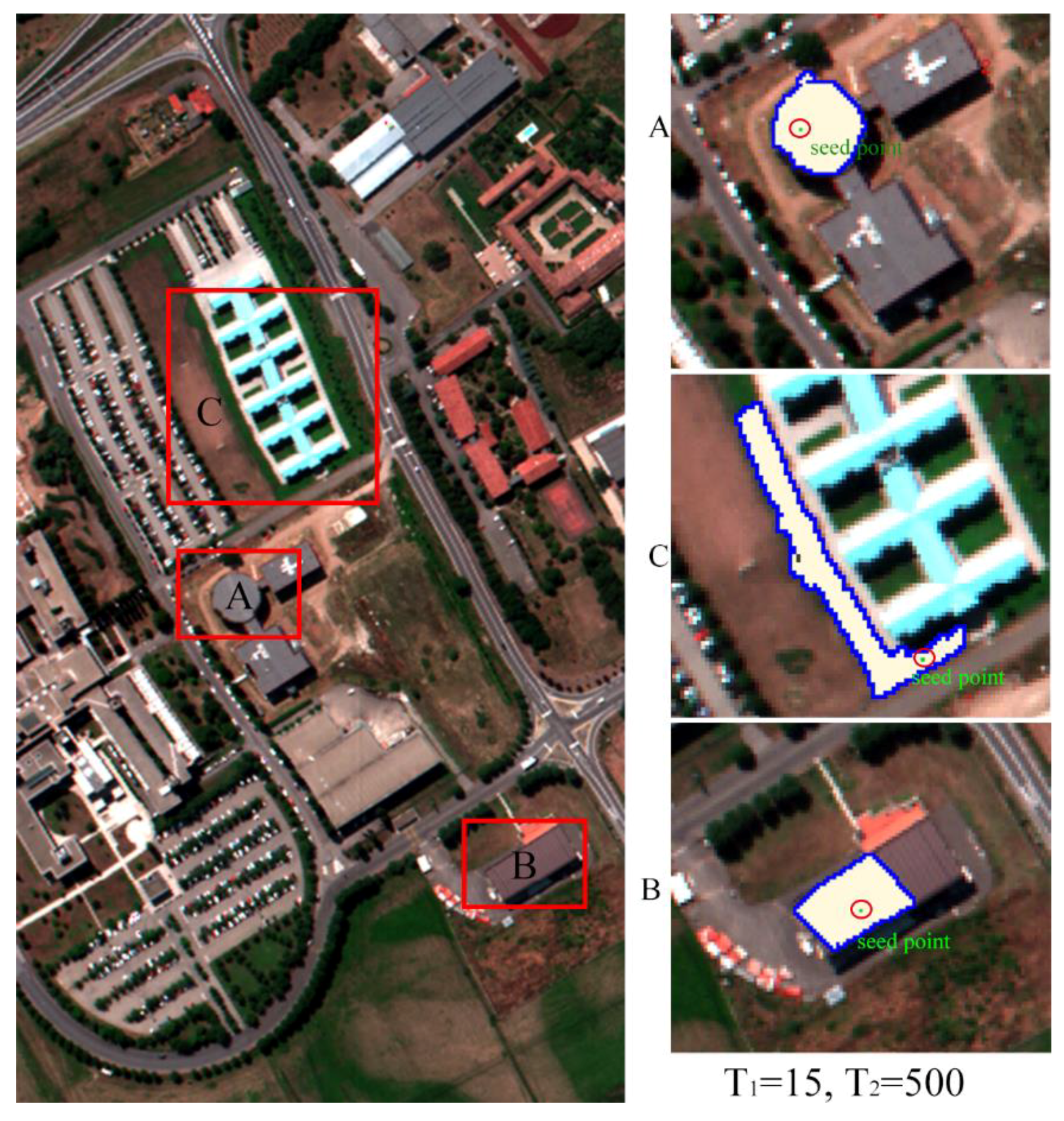
Remotesensing 10 01238 g001
Figure 2. Examples of adaptive regions for the proposed D-AMVS. The green points inside the red circles are the central pixels of each extension, and the blue borders define the shape of the adaptive region: (A,B) are the examples of adaptive region when the central point in the buildings with different shape; (C) is the example of adaptive region when the central point in the meadows.
Remotesensing 10 01238 g002
Figure 3. Pavia University image used in the first experiment: (a) false color original image of Pavia University and (b) ground reference data.
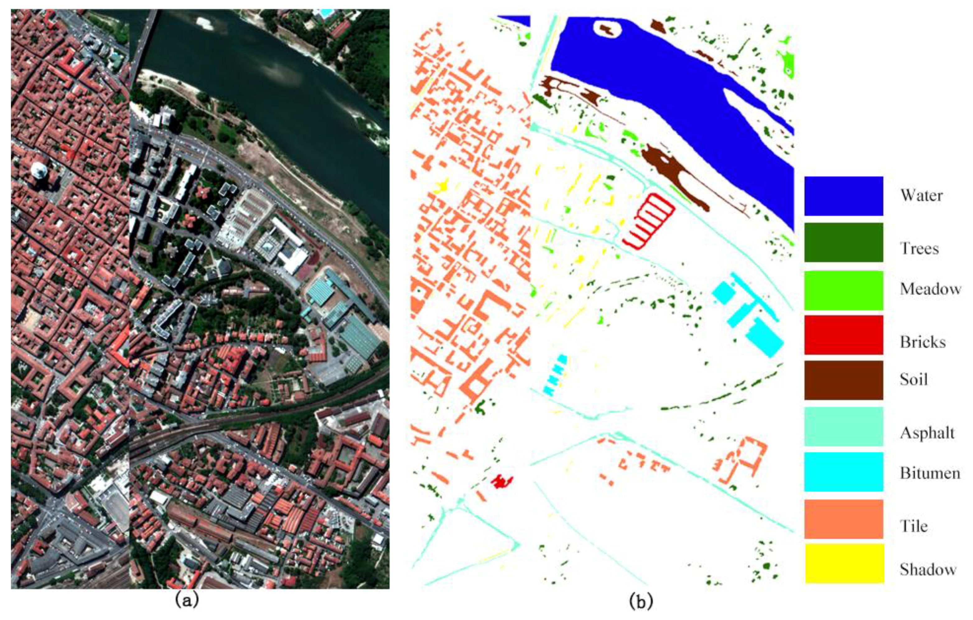
Remotesensing 10 01238 g003
Figure 4. Pavia Center image used in the second experiment: (a) false color original image of Pavia Center and (b) ground reference data.
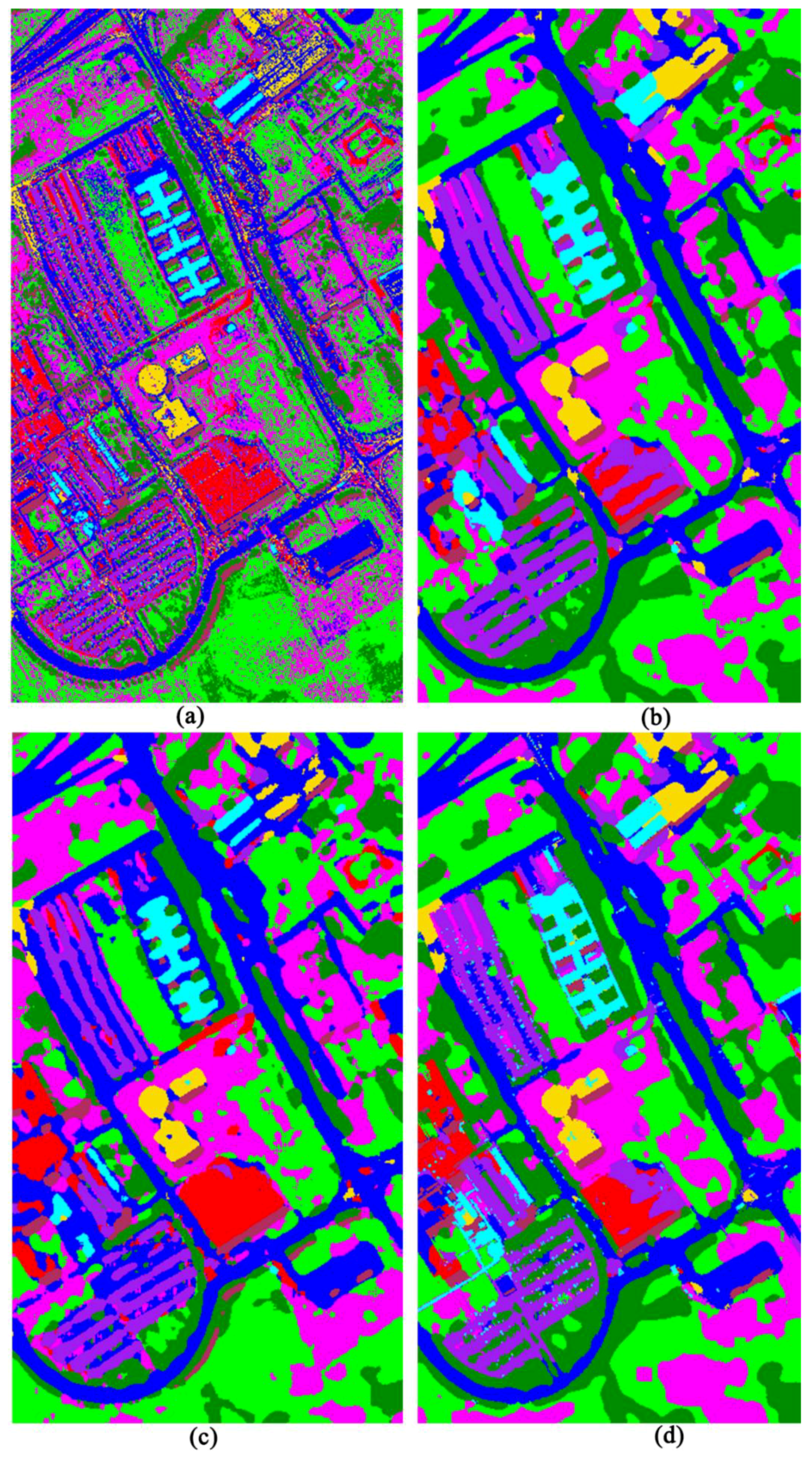
Remotesensing 10 01238 g004
Figure 5. Comparison based on the initial classified maps and different post-classification approaches for the Pavia University image: (a) initial classification map based on the MLC classifier, (b) post-classification map acquired by GPCF with a 9 × 9 window size, (c) post-classification map acquired by majority voting with a 9 × 9 window size, and (d) post-classification map acquired by the proposed D-AMVS with T1 = 60 and T2 = 80.
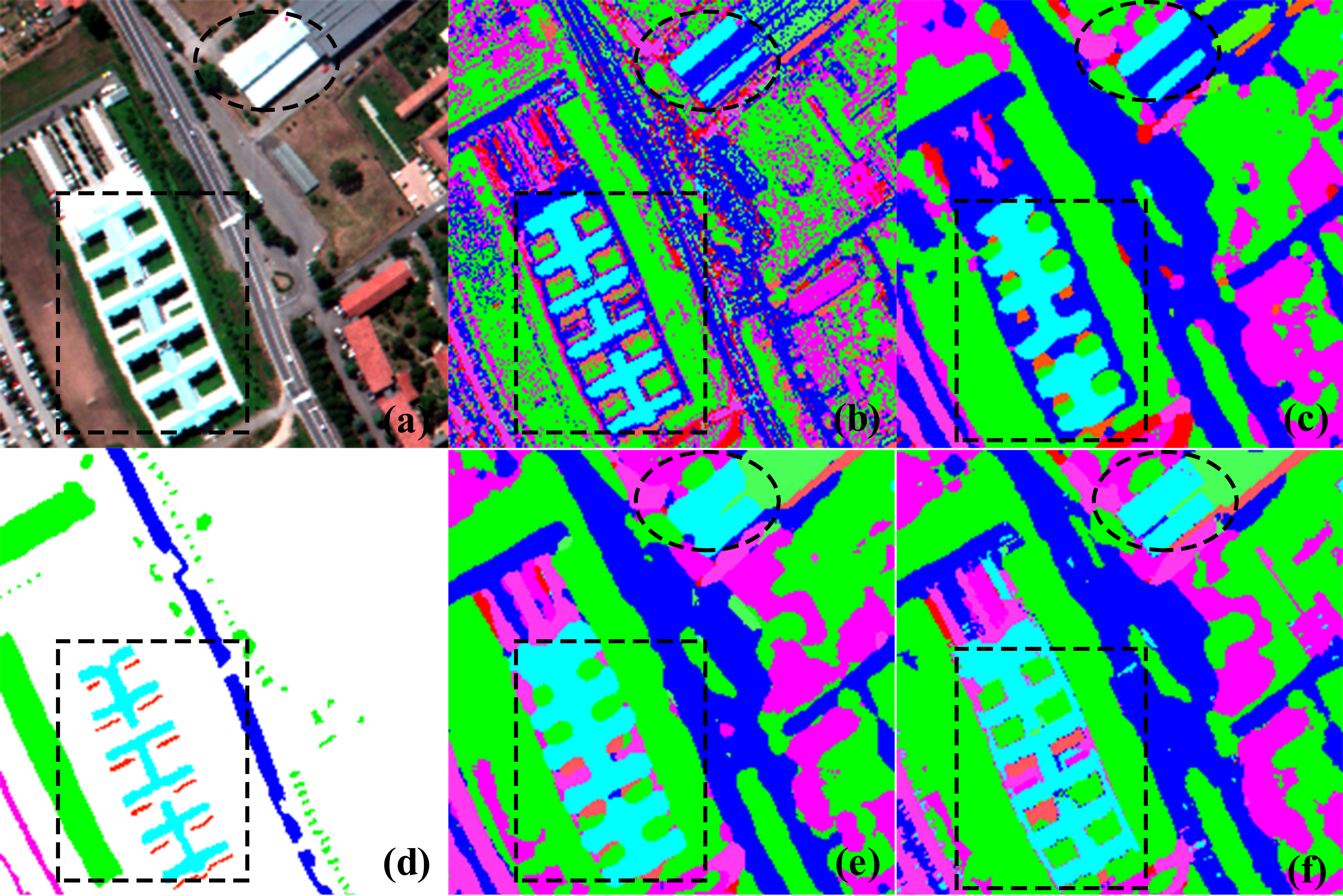
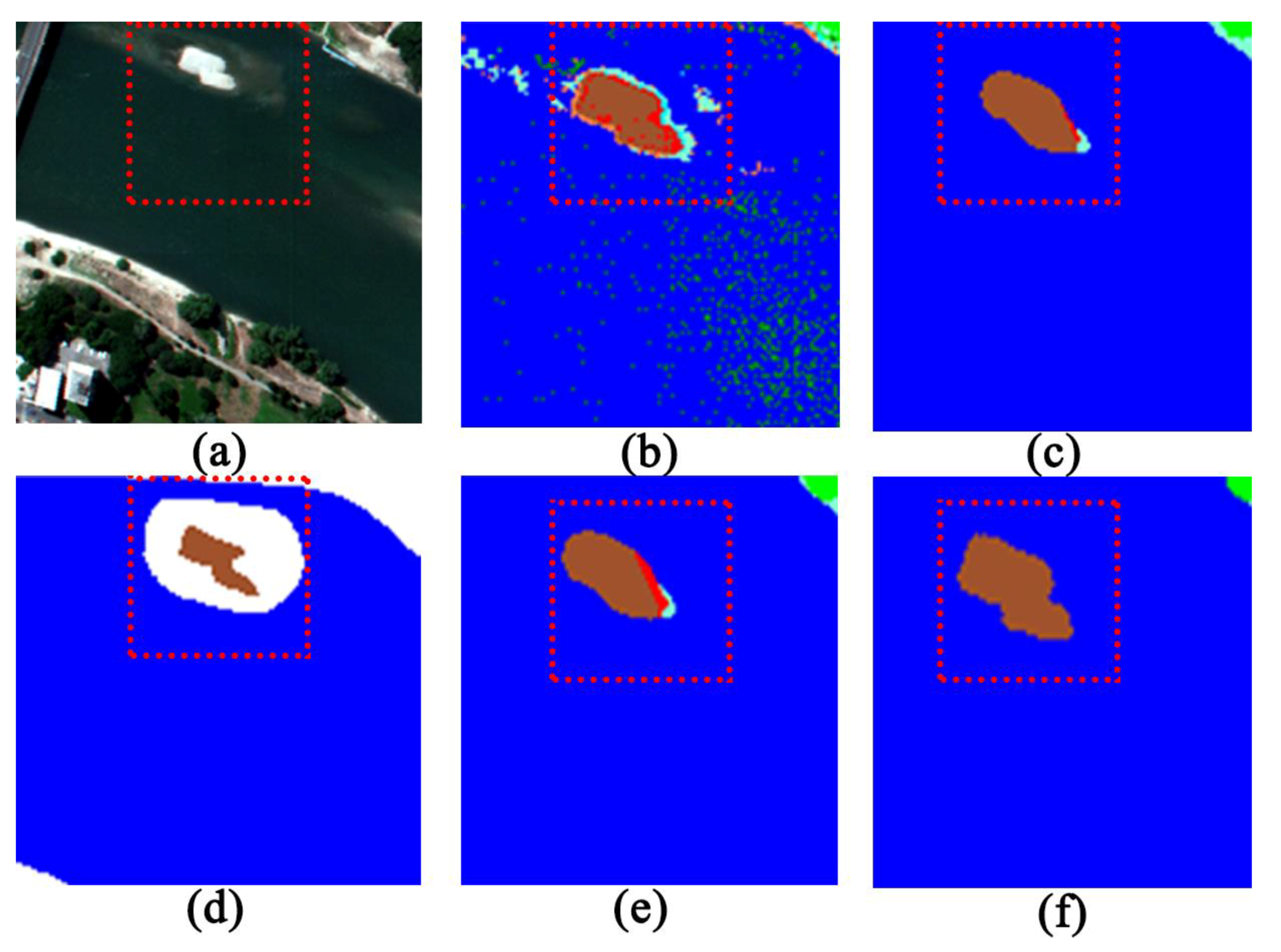
Remotesensing 10 01238 g005
Figure 6. Zoomed comparisons based on the subfigures: (a) Pavia University image, (b) initial classified map obtained by the MLC classifier, (c) post-classification map obtained by GPCF with a 9 × 9 window size, (d) ground reference data, (e) post-classification map acquired by the majority voting approach with a 9 × 9 window size, and (f) post-classification map acquired by the proposed D-AMVS with T1 = 60 and T2 = 80.
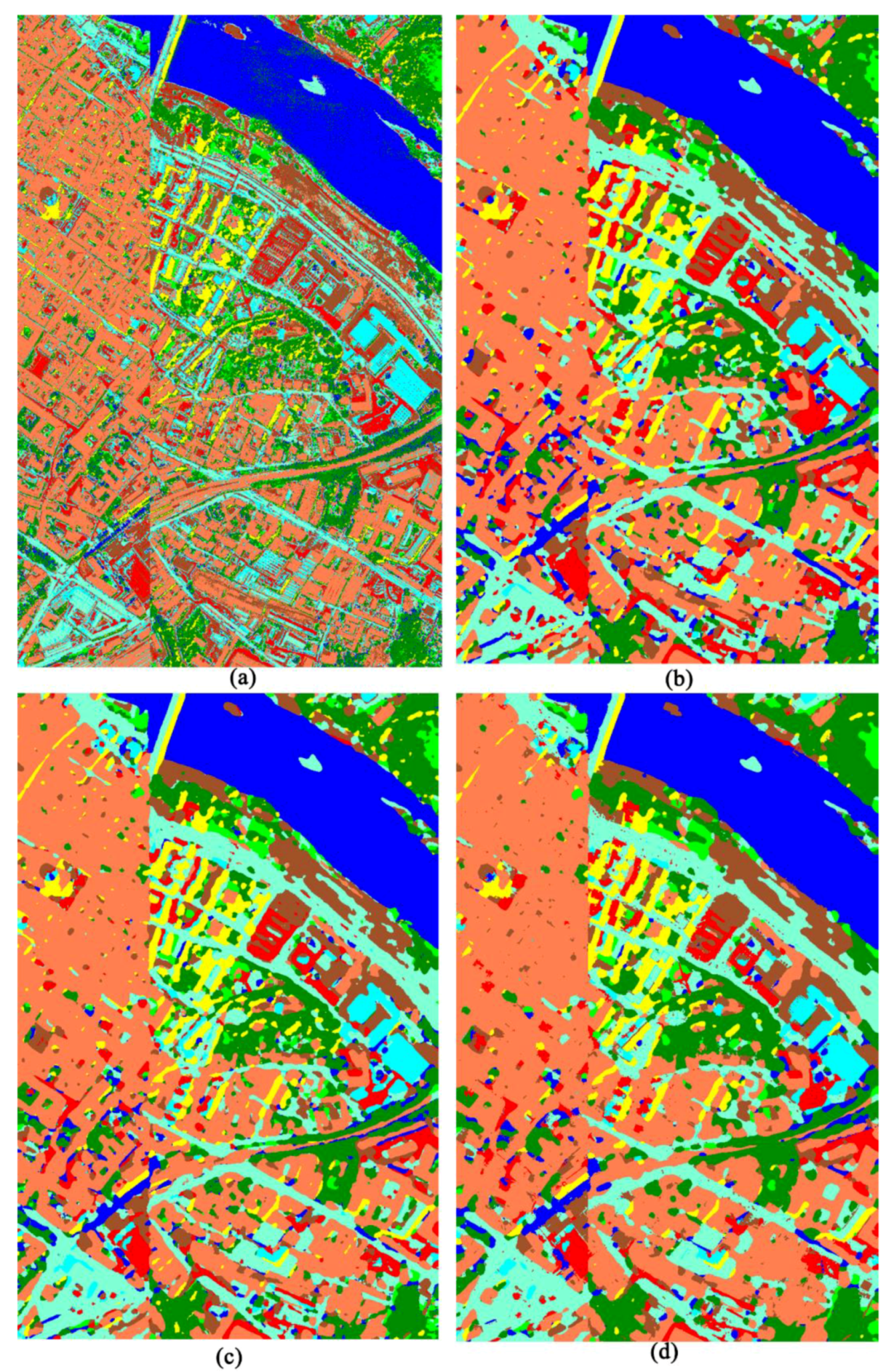
Remotesensing 10 01238 g006
Figure 7. Comparison based on initial classified maps and different post-classification approaches for the Pavia Center image: (a) initial classified map based on RGV spatial–spectral method and SVM classifier, (b) post-classification map acquired by majority voting with a 9 × 9 window size, (c) post-classification map acquired by GPCF with a 9 × 9 window size, and (d) post-classification map acquired by the proposed D-AMVS with T1 = 70 and T2 = 80.
Remotesensing 10 01238 g007
Figure 8. Zoomed comparisons based on the subfigures: (a) Pavia Center image, (b) initial classified map based on RGV spatial–spectral method and SVM classifier, (c) post-classification map obtained by GPCF with a 9 × 9 window size, (d) ground reference data, (e) post-classification map acquired by majority voting with a 9 × 9 window size, and (f) post-classification map acquired by the proposed D-AMVS with T1 = 70 and T2 = 80.
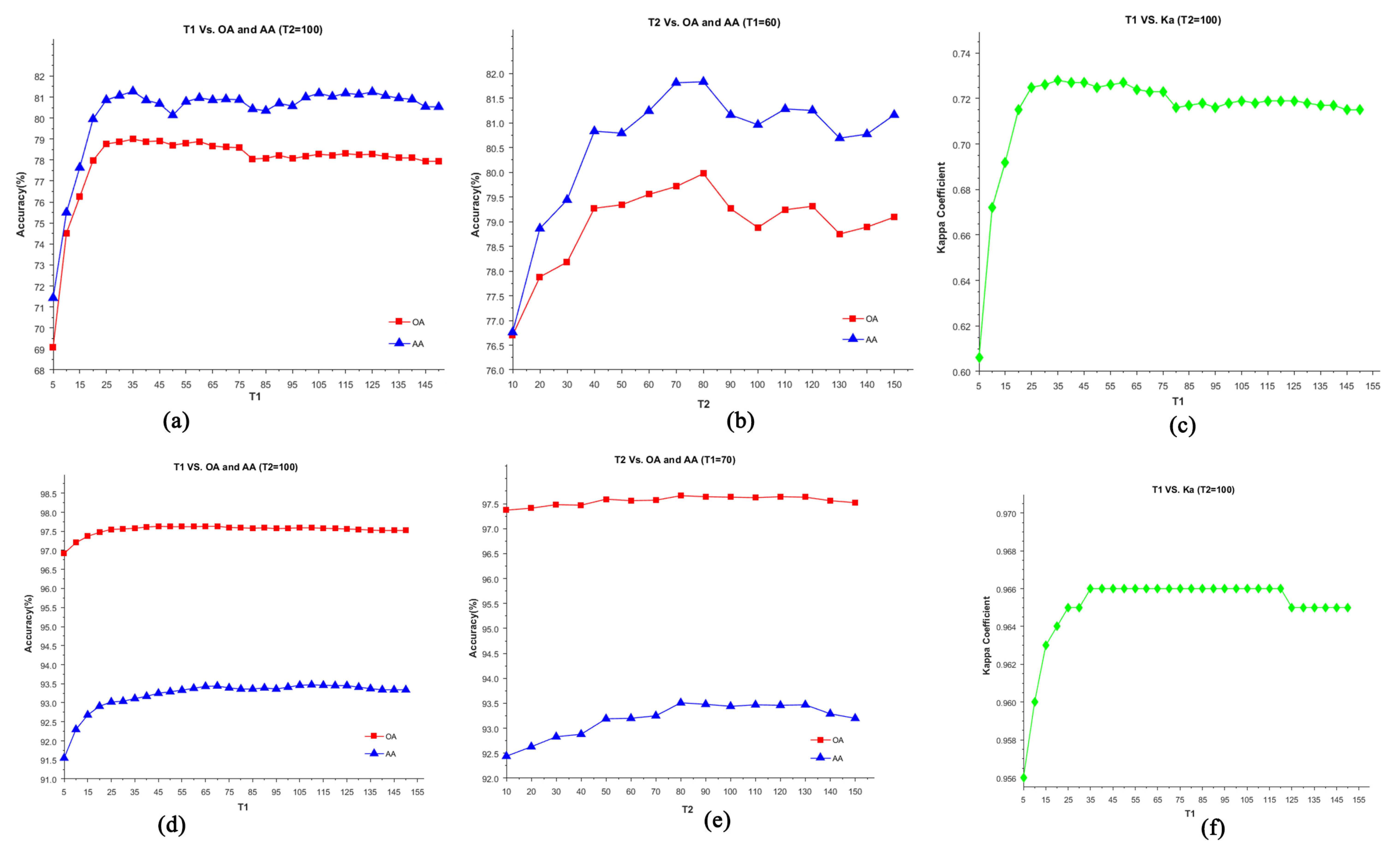
Remotesensing 10 01238 g008
Figure 9. Relationship between classification maps and parameter settings (T1 and T2) of the proposed D-AMVS method: (ac) are the relationships between T1, T2, and OA/AA/Ka, respectively, for the Pavia University image, and (df) present the relationships between T1, T2, and OA/AA/Ka for the Pavia Center image, respectively.
Remotesensing 10 01238 g009
Table 1. Number of training samples and reference data for the Pavia University image.
ClassTraining SamplesTest Samples
Asphalt6036631
Meadows39618,649
Gravel1822099
Trees3823064
Painted metal461345
Bare soil6805029
Bitumen1891330
Self-blocking bricks4143682
Shadows88847
Table 2. Number of training samples and reference data for the Pavia Center image.
ClassTraining SamplesTest Samples
Water62365,971
Trees3367598
Meadows1233090
Bricks2932685
Soil2896584
Asphalt4009248
Bitumen2217287
Tiles63842,826
Shadows3792863
Table 3. Initial classification results acquired by different classifiers for the Pavia University image. OA: overall accuracy, Ka: Kappa coefficient, AA: average accuracies, NN: neural network, MLC: maximum likelihood classification, MD: Mahalanobis distance, SVM: support vector machine.
NNMLCMDSVM
OA (%)47.2167.5953.6660.92
Ka0.38240.58980.42600.517
AA (%)51.5869.2256.6365.39
Table 4. Comparison of the proposed D-AMVS and different post-classification approaches for the Pavia University image. GPCF: general post-classification framework.
Window SizeMajority VotingGPCFProposed D-AMVS
35793579T1 = 60, T2 = 80
OA (%)73.2475.6877.0878.1170.2571.9672.7373.279.97
Ka0.6590.6890.7070.720.6260.6470.6570.6630.741
AA (%)74.6377.2678.8180.0872.4875.4777.3878.4681.83
Table 5. Class-specific user accuracy (%) of the Pavia University image for the different methods.
MLCMV
( w = 5 × 5 )
GPCF
( w = 5 × 5 )
D-AMVs
(T1 = 60, T2 = 80)
Asphalt79.086.292.990.9
Meadows83.886.895.087.9
Gravel44.164.378.089.1
Trees61.066.952.960.2
Painted metal95.896.093.593.7
Bare soil33.040.736.151.3
Bitumen54.572.567.782.9
Self-blocking bricks74.282.673.380.5
Shadows97.599.499.8100
Table 6. Initial classified image acquired by different spectral–spatial approaches and the SVM classifier for the Pavia Center image. EMPs: extended morphological profiles, M-EMPs: multi-shape extended morphological profiles, RF: recursive filter, RGF: rolling guidance filter.
EMPs [26] M-EMPs [25]RF [28]RGF [43]
OA (%)96.0495.5193.5196.72
Ka0.9440.9370.9090.954
AA (%)88.8287.282.2591.06
Table 7. Comparisons of the proposed D-AMVS and different post-classification approaches for the Pavia Center image.
Window SizeMajority VotingGPCFProposed D-AMVS
35793579T1 = 70, T2 = 80
OA (%)96.8496.9697.0297.0497.4197.4697.597.5597.66
Ka0.9550.9570.9580.9580.9630.9640.9650.9650.967
AA (%)91.4291.8192.0292.1592.4792.6392.8493.0993.51
Table 8. Class-specific user accuracy of the Pavia Center image for the different methods.
RGF [43]Majority Voting
( w = 5 × 5 )
GPCF
( w = 5 × 5 )
D-AMVS
(T1 = 70, T2 = 80)
Water99.299.199.699.7
Trees97.597.398.697.7
Meadows88.889.788.091.5
Bricks66.067.867.171.0
Soil89.191.997.997.7
Asphalt86.486.888.188.8
Bitumen93.294.395.898.0
Tiles99.999.999.799.3
Shadows99.599.698.898.0
Table 9. Error estimation among the different methods for the Pavia Center image data.
D-AMVS
OA (%)KappaAA (%)
RGF0.940.0132.45
Majority Voting0.820.0122.09
GPCF0.250.0041.04
Table 10. Error estimation between the proposed D-AMVS and majority voting approach in terms of user accuracy for the Pavia Center image data.
D-AMVS (T1 = 70, T2 = 80)
WaterTreesMeadowsBricksSoilAsphaltBitumenTilesShadow
Majority Voting
( w = 5 × 5 )
Water2460000−246000
Trees−5322−62052702932
Meadows−2317−17008−4109
Bricks000269−2634−1000
Soil0−10191−176−4−1200
Asphalt−930062311−23040
Bitumen−1100−2431519209110
Tiles−6−2304−142−1101780
Shadows−192−21000160203−6
User accuracy error (%)0.60.41.83.25.823.7−0.6−1.6

