Distributed Fiber Optic Sensors for the Monitoring of a Tunnel Crossing a Landslide

Abstract

This work reports on the application of a distributed fiber-optic strain sensor for long-term monitoring of a railway tunnel affected by an active earthflow. The sensor has been applied to detect the strain distribution along an optical fiber attached along the two walls of the tunnel. The experimental results, relative to a two-year monitoring campaign, demonstrate that the sensor is able to detect localized strains, identify their location along the tunnel walls, and follow their temporal evolution.

1. Introduction

Optical fiber distributed sensors have recently gained great attention in structural and environmental monitoring. Besides sharing the advantages of all fiber-optic sensors (immunity to electromagnetic interference, high sensitivity, small size, the possibility to be embedded into structures, multiplexing, and remote interrogation capabilities [1]), they also offer the unique feature of allowing the exploitation of a telecommunication grade optical fiber as the sensing element, covering long distances with high spatial resolution without any added devices. In fact, distributed optical fiber sensors based on stimulated Brillouin scattering allow measurement of the strain and temperature profiles with a typical spatial resolution of 1 m (or less) and a measurement range of up to tens of kilometers. These sensors have already been employed in static and dynamic monitoring of a variety of structures allowing identification of the deformation field and localization of failures [2,3,4,5,6,7,8,9,10,11].

This paper deals with the application of the Brillouin Optical Time-Domain Analysis (BOTDA) to the monitoring of the deformations of a railway tunnel located in the accumulation zone of an active earthflow in the Southern Italian Apennines. The landslide movements caused severe damage to the original tunnel which, built in 1880, had to be reconstructed about a century later, in 1992. Since then, the new impressive structure bears the earth thrust and undergoes limited damage, notwithstanding the activity of the landslide. In fact, an average displacement rate of about 1 cm/year has been measured in the last 14 years in the accumulation zone of the landslide, as a result of sliding on two slip surfaces (20 m and 40 m deep, respectively) and internal deformations. From the time of reconstruction, the Italian National Railway has periodically monitored the opening of the joints and of some thin cracks. Recently, thanks to a collaboration with the Rail Infrastructure Manager (RFI), the tunnel is being monitored with optical fiber distributed sensors and frequent direct inspections are being carried out. This paper presents the results of the optical fiber monitoring over two years by a sensing cable simply glued to the tunnel walls. The possibility has been checked to detect localized fiber strains, to identify their location along the tunnel walls and to follow their temporal evolution. The paper is organized as follows: In the next section, we will provide the fundamentals of distributed sensing based on BOTDA. Therefore, we will present the history of the landslide and discuss the results of the monitoring campaign. Conclusions will follow.

2. Distributed Fiber Optic Strain Sensing

Distributed optical fiber sensors based on stimulated Brillouin scattering (SBS) retrieve the strain (or temperature) profile along the fiber, through the measurement of the so-called Brillouin Frequency Shift (BFS). The BFS is a parameter related to the optical and elastic properties of the fiber, and this measurement is carried out typically by adopting the so-called Brillouin Optical Time-Domain Analysis (BOTDA). In the latter, a continuous wave probe signal and a frequency-shifted, pulsed pump signal are injected at the two opposite ends of the fiber. When the optical frequencies of the two waves differ from a quantity close to the BFS of the fiber (~11 GHz for systems operating at 1.55 µm wavelength), an intense acoustic wave is generated from the interference pattern created by the two optical waves through the phenomenon of electrostriction. The acoustic wave acts as a diffraction grating, backscattering part of the pump energy in favor of the probe wave. As a result, the fiber behaves as an active medium pumped by the pump pulse, amplifying the probe wave as it travels along the fiber itself. The gain experienced by the probe wave has a typical Lorentzian dependence on the pump-probe frequency shift, reaching its maximum when the latter matches the BFS of the fiber. As the BFS varies linearly with strain (and temperature), the fiber acts as a sensor for these parameters. From a practical point of view, the Brillouin gain is measured as a function of time starting from the injection of the pump pulse. As the group velocity of the latter is known, it is easy to convert the time coordinate into a spatial one, thus providing a mechanism to resolve the BFS in different positions along the fiber. The spatial resolution, i.e., the capability of the sensor to discriminate between temperature/strain changes in different positions of the fiber, is proportional to the pump pulse duration, with a conversion factor of 1 m/10 ns.

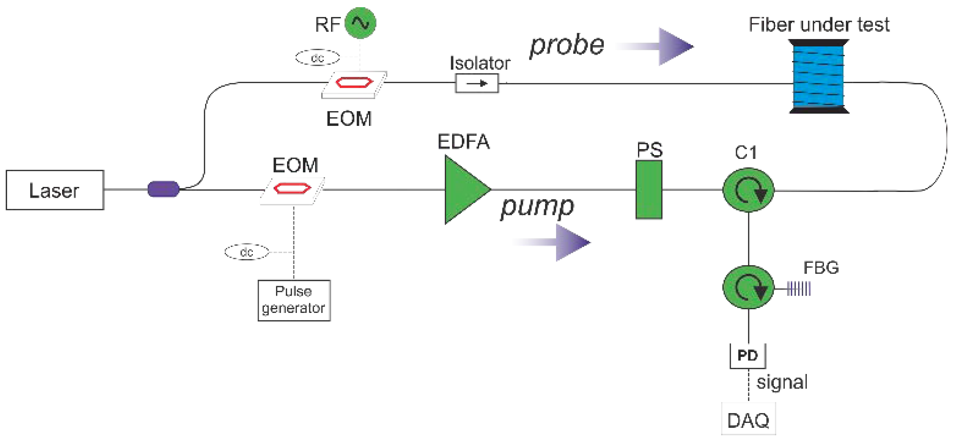
The measurements presented in this paper have been carried out using a portable instrument, implementing the scheme illustrated in Figure 1.

Light from a 1.55 µm distributed feedback (DFB) laser diode is split into two arms to generate the pump (lower branch) and the probe (upper branch) fields. The two optical fields are frequency-shifted by means of an electro-optic modulator (EOM) inserted in the probe branch, in order to realize a double sideband, carrier-suppressed modulation. At the modulator output, the optical probe wave consists of two tones; each one shifted from the carrier of a quantity equal to the RF frequency generated by the EOM driver. The sideband with lower frequency acts as the probe beam, while the upper sideband is filtered out through a fiber Bragg grating (FBG) placed before the detector. On the pump branch, the pump field is pulsed by another electro-optic modulator driven by a pulse generator. The pump pulse is amplified by an erbium-doped fiber amplifier (EDFA) and then passed through a polarization scrambler operating at a 700 kHz scrambling rate, aimed to average out the Brillouin gain fluctuations due to fiber birefringence. Note that the same FBG employed for the suppression of the upper sideband of the probe wave, also acts as a bandpass filter for the Amplified Spontaneous Emission (ASE) noise produced by the EDFA. Finally, the intensity of the probe wave emerging from the fiber being tested is detected by a high-speed photodetector whose output is connected to a data acquisition card (DAQ) with a sampling rate of 250 MS/s. The measurement process involves the measurement of the probe gain as a function of time, for a range of pump-probe frequency shifts, whose values are scanned through the RF generator connected to the EOM in the probe branch. Typically, the RF frequency is scanned from 10,500 MHz to 11,500 MHz with a 2 MHz frequency step. Furthermore, for each given RF frequency the probe gain waveform is acquired and accumulated several times, in order to increase the signal-to-noise ratio. For the measurements shown in this paper, we set a number of 2048 accumulations, and a pulse duration of 10 ns. These settings allowed for a spatial resolution of 1 m, and a BFS accuracy of ±1 MHz, with the latter corresponding to a strain accuracy of ±20 µε.

3. The Varco d’Izzo Earthflow

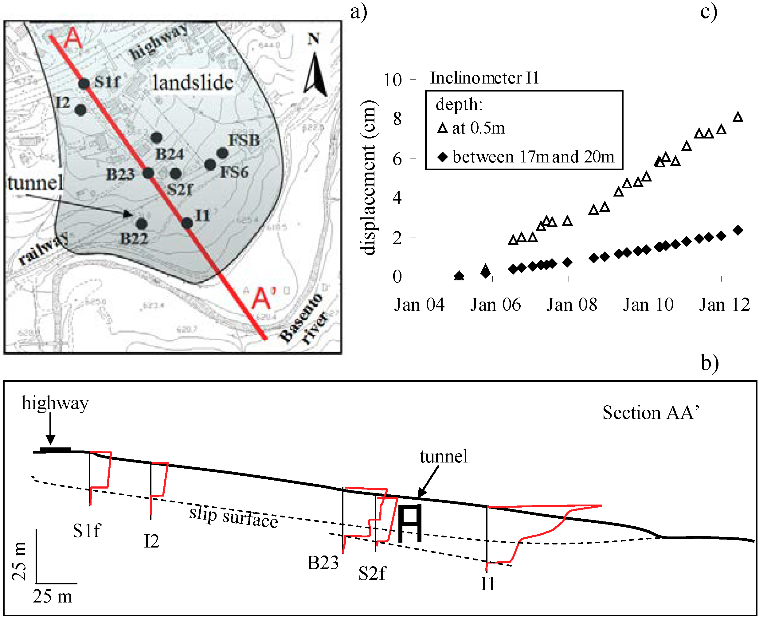
The optical fiber monitoring system described above was installed in the railway tunnel crossing the accumulation of an active earthflow in a highly tectonized clay shale deposit, which is part of the Varicoloured Clays formation [12]. The earthflow, shown in Figure 2a, is located in the eastern suburbs of the town of Potenza (Southern Italy) and belongs to a large and complex landslide system [13], extending over an area of about 1 km², which causes frequent damage to residential buildings, internal roads, and the national highway. A number of geotechnical investigations, including displacement monitoring by inclinometers and GPS, have been carried out in the entire area over the last 25 years and thus the main features of the landslide phenomena have been described [13,14,15,16,17]. Figure 2b shows two slip surfaces which have been detected thanks to inclinometer readings. The shallowest, about 20 m deep, seems to intersect the piles of the tunnel; however, the inclinometer displacement profiles obtained 10–15 years ago in the vicinity of the upslope tunnel side did not reveal shear displacements at the depth of such a slip surface, suggesting that the piles were still intact. On the contrary, in the subsoil downslope from the tunnel and on the same slip surface, shear displacements were observed at a quite constant yearly rate—only with seasonal variations—over the whole monitoring period, as shown in Figure 2c.

The other inclinometers of the landslide system did not show significant temporal changes in the displacement rate [13]. Furthermore, some permanent and non-permanent GPS stations provided ground displacements in agreement with the inclinometer readings [18,19]. In particular, a station placed in proximity to the western end of the tunnel underwent ground displacements in the order of 1 cm/year.

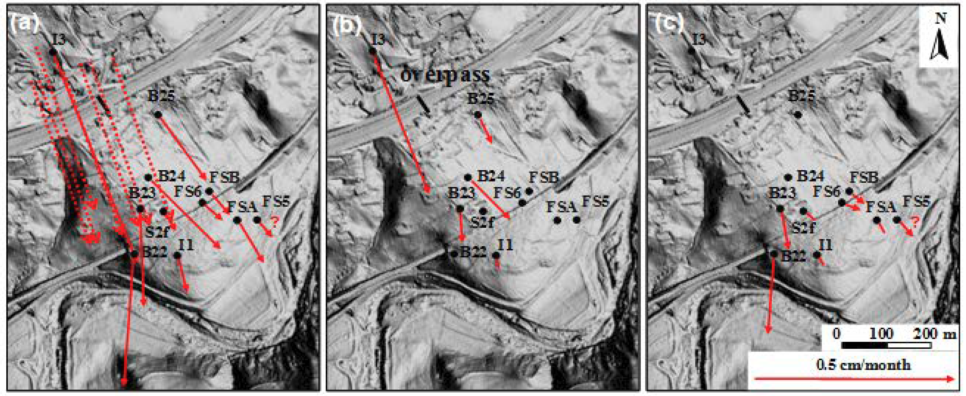
Figure 3a shows ground displacements, Figure 3b shows shear displacements along the shallower slip surface, and Figure 3c shows shear displacements on the deeper slip surface. Figure 3a also shows the results of a topographic survey which was carried out by an automated total station located upslope from the tunnel, in the area around the inclinometer, I3. It is worth noting that, upslope from the tunnel, the rate of ground displacement decreases in the downslope direction, thus revealing the effective retaining role of the tunnel with its piles.

4. The Tunnel Monitoring

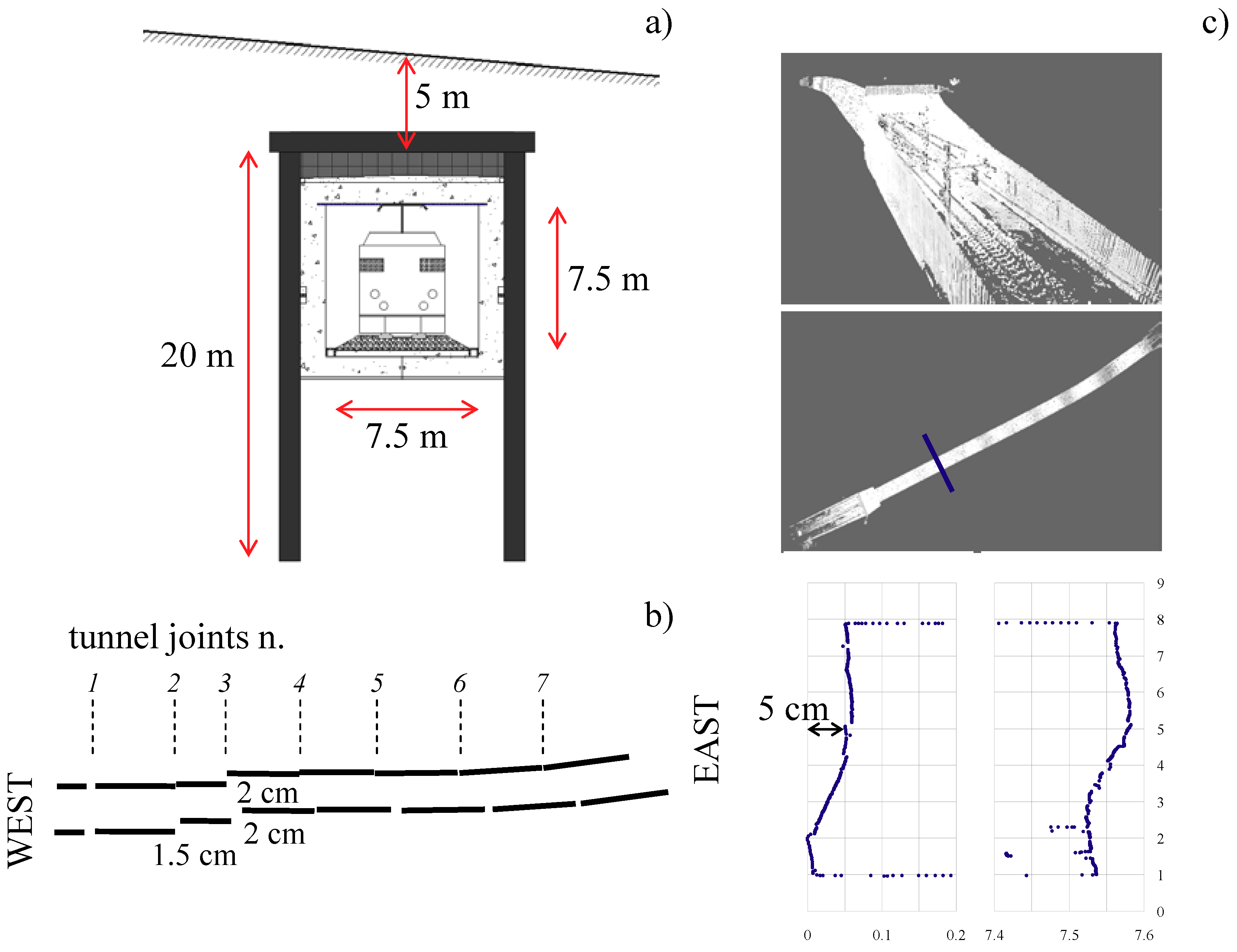
The tunnel, re-built in 1992, is an artificial tunnel, flanked by two sheet pile walls having the goal to assure safe excavation works. A schematic drawing is shown in Figure 4a. The structure, 200 m long, consists of eight contiguous sectors separated by joints with irregular spacing, as shown in Figure 4b. The internal structure is a reinforced concrete box with a thickness of 1 m and a 7.5 × 7.5 m square section. The sheet pile walls are made of contiguous piles, with a diameter of 1 m and a length of 20 m. The piles are adjacent but not linked to the concrete box.

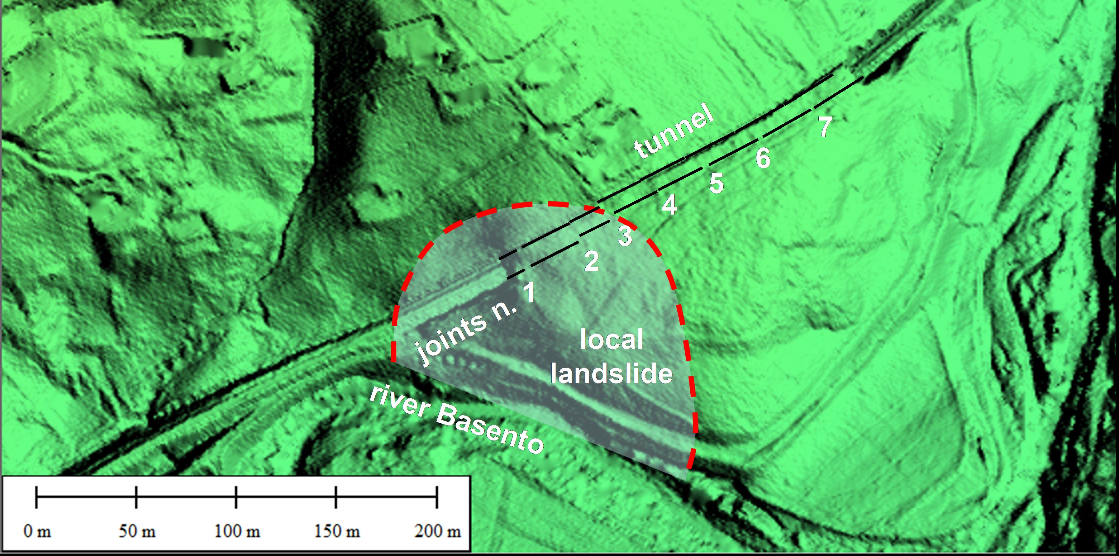
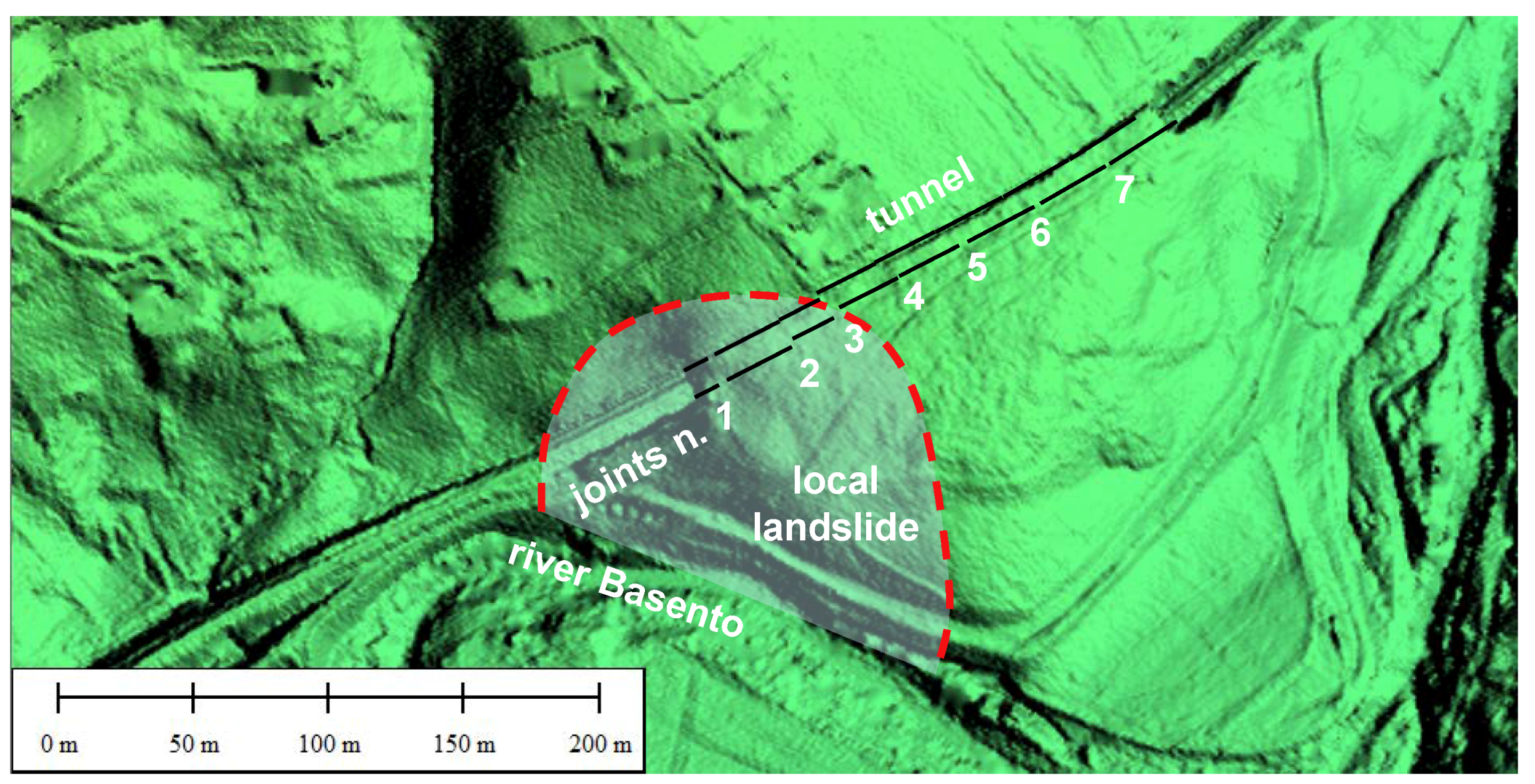
In October 2015, a high definition survey of the tunnel’s internal geometry was carried out via 3D laser scanning, as shown in Figure 4c. The use of such a technique allowed for the reconstruction of the geometry of vertical cross sections of the tunnel, revealing that some of them, especially near the western end, display a horizontal drift of about 5 cm between the base and the roof [17]. Such a deformed shape corresponds to what can be expected due to unbalanced actions of pressure from the earth acting on the walls. However, the most important deformations have been detected in joints 1, 2, and 3, again at the western entrance of the tunnel, as shown in Figure 4b. It is worth noting that this part of the tunnel is affected by a local lateral landslide, which occurs within the main earthflow, triggered by the Basento river erosion, see Figure 5. The intersection of the boundary of the local landslide with the tunnel occurs close to joint 3, where the largest misalignment of the adjacent sectors, in the order of 2 cm, has been evaluated. Slightly lower misalignments have been evaluated in relation to joints 1 and 2. Under the hypothesis of a constant rate, a 0.5 mm/year opening can be inferred for the two joints since the year of construction (1992).

5. Results of Optical Fiber Monitoring

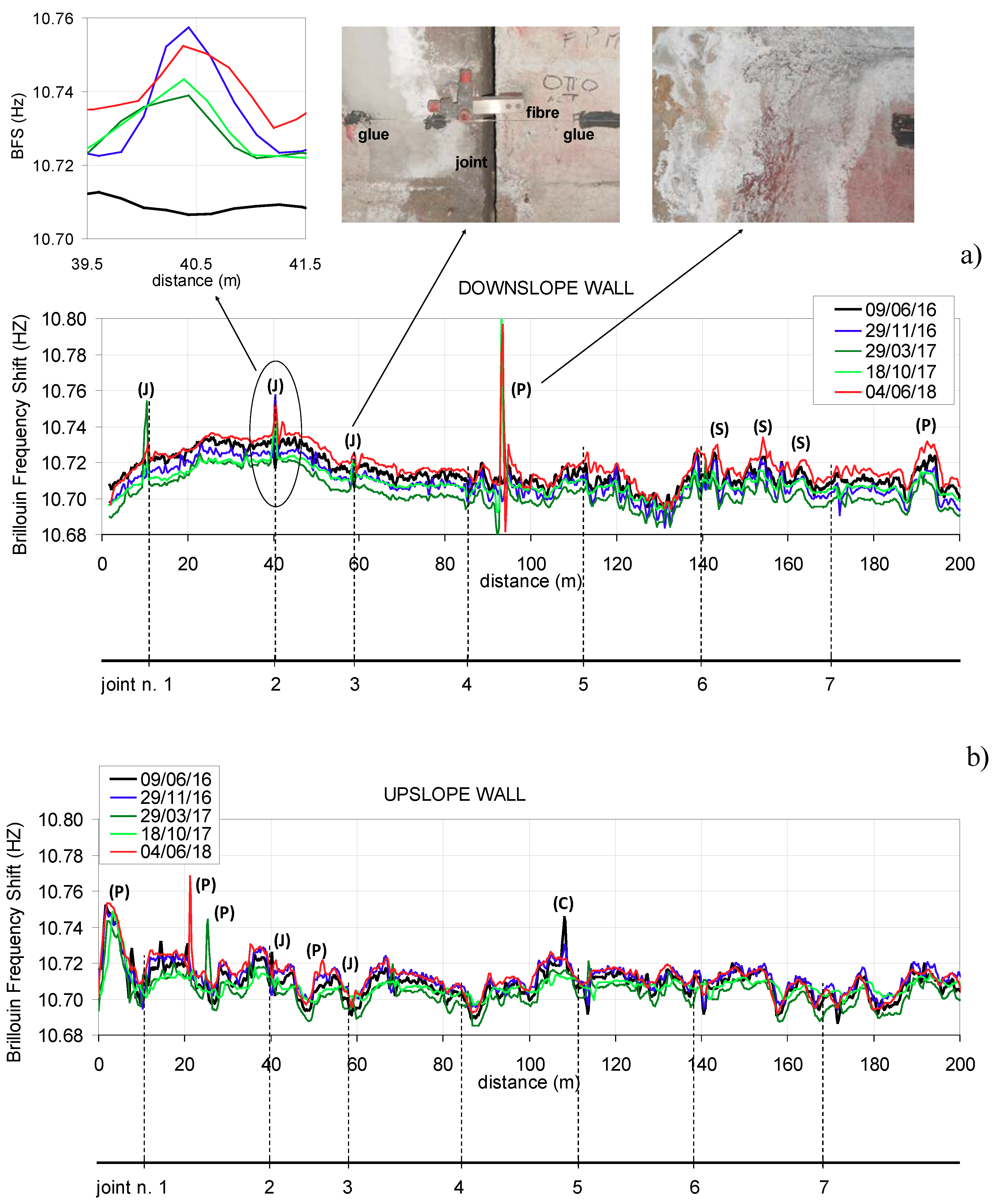
The optical fiber monitoring was carried out through the setup described in Section 2. The sensing element constituted of a conventional single-mode optical fiber with a 900 µm tight buffer, hand-glued along the two walls of the tunnel. The first “zero” reading was carried out on the 9th of June 2016. The results of this reading, as well as those of subsequent measurements (from the 23rd of November 2016 to the 4th of June 2018), are shown in Figure 6, where each BFS profile is provided by a sensor with a 20 cm spacing. The figure also indicates the position of the structural joints. We note that the BFS profiles exhibit some irregularity, which is essentially due to the strain induced on the fiber by the gluing procedure. In fact, most of these irregularities exhibit the same behavior for each measurement. Apart from this, the BFS profiles also exhibit a number of peaks. Several successive inspections in the tunnel revealed that these peaks correspond to four different phenomena, indicated by a bracketed letter in Figure 6. The letter J corresponds to a joint opening; this phenomenon occurred in the same locations in which it has occurred in the past, i.e., in joints 1, 2 and 3, as discussed in Section 4. The letter C corresponds to a crack of the tunnel wall. The letter P corresponds to local deformations of the walls due to parget swelling, and the letter S to salt precipitate accumulation due to water infiltration.

The temporal trend of the joint opening as revealed by the fiber system is shown in Figure 7. The elongations were obtained by inspecting the BFS variation along a fiber section of 1 m around each joint. In detail, the procedure used to calculate elongations is as follows: First, from each measurement we have subtracted the BFS profile acquired on the 9th of June 2016, in order to extract only the variations of the BFS compared to the zero reading; then, we have converted the BFS changes in strain values, by adopting a BFS/strain transduction coefficient of 20 µε/MHz. Third, we have performed a de-trending of the strain profile in order to remove artifacts due to gluing-induced strain. Fourth, the de-trended strain profile was vertically shifted in order to move the baseline to zero and therefore compensate for temperature-induced BFS changes. Finally, the slope-corrected and vertically-shifted strain profile associated with each joint was numerically integrated, in order to determine the longitudinal elongation at that joint.

The increase in joint opening/misalignment provided by the fiber elongation is very small but significant for the structure, as shown in Figure 7. The increase is more pronounced in the downslope wall of the tunnel, consistent with the fact that the local landslide responsible for the structural instability is triggered by the river erosion. Furthermore, the opening phenomenon is not linear; over the monitoring time, the shift has been concentrated in the winter between 2016 and 2017, when the inclinometers of the area also recorded an acceleration in the landslide movements. Although these are the first results of fiber-based monitoring of the structure, they can be already considered a reliable pre-alert, which requires prevention interventions.

6. Conclusions

A monitoring campaign has been carried out exploiting a distributed optical fiber sensor installed along the walls of a railway tunnel. The results indicate the ability of the sensor to remotely detect and locate several phenomena occurring along the fiber path, one of which is the opening of the structure joints, with misalignment. Furthermore, the analysis of the experimental data shows that the fiber system can also be used for evaluating the time evolution of the deformation. Thus, the fiber system seems to represent a useful monitoring system that, if operated on a time-continuous basis, can also be used to pre-alert. Moreover, based on these first results, new and more efficient fiber systems can be designed and installed.