Next Article in Journal
Fractal-Based Local Range Slope Estimation from Single SAR Image with Applications to SAR Despeckling and Topographic Mapping
Previous Article in Journal
Symmetric Double-Eye Structure in Hurricane Bertha (2008) Imaged by SAR
 
 
Correction published on 26 March 2019, see Remote Sens. 2019, 11(6), 726.
Article

Using Near-Infrared-Enabled Digital Repeat Photography to Track Structural and Physiological Phenology in Mediterranean Tree–Grass Ecosystems

by Yunpeng Luo 1,*, Tarek S. El-Madany 1, Gianluca Filippa 2, Xuanlong Ma 1, Bernhard Ahrens 1, Arnaud Carrara 3, Rosario Gonzalez-Cascon 4, Edoardo Cremonese 2, Marta Galvagno 2, Tiana W. Hammer 1, Javier Pacheco-Labrador 1,5, M. Pilar Martín 5, Gerardo Moreno 6, Oscar Perez-Priego 1, Markus Reichstein 1,7, Andrew D. Richardson 8,9,10, Christine Römermann 11,12 and Mirco Migliavacca 1
1
Department for Biogeochemical Integration, Max-Planck-Institute for Biogeochemistry, 07745 Jena, Germany
2
Environmental Protection Agency of Aosta Valley, ARPA Valle d’Aosta, 11020 Aosta, Italy
3
Fundación Centro de Estudios Ambientales del Mediterráneo (CEAM), 46980 Paterna, Spain
4
Department of Environment, National Institute for Agriculture and Food Research and Technology (INIA), 28040 Madrid, Spain
5
Environmental Remote Sensing and Spectroscopy Laboratory (SpecLab), Spanish National Research Council (CSIC), 28037 Madrid, Spain
6
Institute for Dehesa Research, University of Extremadura, 10600 Plasencia, Spain
7
Michael-Stifel-Center Jena for Data-Driven and Simulation Science, 07743 Jena, Germany
8
Department of Organismic and Evolutionary Biology, Harvard University, Cambridge, MA 02138, USA
9
School of Informatics, Computing and Cyber Systems, Northern Arizona University, Flagstaff, AZ 86011, USA
10
Center for Ecosystem Science and Society, Northern Arizona University, Flagstaff, AZ 86011, USA
11
Institute of Ecology and Evolution, Plant Biodiversity Group, Friedrich Schiller University Jena, 07743 Jena, Germany
12
German Centre for Integrative Biodiversity Research (iDiv) Halle-Jena-Leipzig, 04103 Leipzig, Germany
*
Author to whom correspondence should be addressed.
Remote Sens. 2018, 10(8), 1293; https://doi.org/10.3390/rs10081293
Submission received: 16 July 2018 / Revised: 8 August 2018 / Accepted: 13 August 2018 / Published: 15 August 2018
(This article belongs to the Section Biogeosciences Remote Sensing)

Abstract

:
Tree–grass ecosystems are widely distributed. However, their phenology has not yet been fully characterized. The technique of repeated digital photographs for plant phenology monitoring (hereafter referred as PhenoCam) provide opportunities for long-term monitoring of plant phenology, and extracting phenological transition dates (PTDs, e.g., start of the growing season). Here, we aim to evaluate the utility of near-infrared-enabled PhenoCam for monitoring the phenology of structure (i.e., greenness) and physiology (i.e., gross primary productivity—GPP) at four tree–grass Mediterranean sites. We computed four vegetation indexes (VIs) from PhenoCams: (1) green chromatic coordinates (GCC), (2) normalized difference vegetation index (CamNDVI), (3) near-infrared reflectance of vegetation index (CamNIRv), and (4) ratio vegetation index (CamRVI). GPP is derived from eddy covariance flux tower measurement. Then, we extracted PTDs and their uncertainty from different VIs and GPP. The consistency between structural (VIs) and physiological (GPP) phenology was then evaluated. CamNIRv is best at representing the PTDs of GPP during the Green-up period, while CamNDVI is best during the Dry-down period. Moreover, CamNIRv outperforms the other VIs in tracking growing season length of GPP. In summary, the results show it is promising to track structural and physiology phenology of seasonally dry Mediterranean ecosystem using near-infrared-enabled PhenoCam. We suggest using multiple VIs to better represent the variation of GPP.

Graphical Abstract

1. Introduction

Phenology is the study of recurring life cycle stages, and their timing and relationship with environmental factors [1,2]. Phenology controls the seasonality of ecosystem functions and plant feedbacks to climate through diverse processes, such as changes in the surface albedo and the exchange of CO2 between atmosphere and biosphere [3,4,5,6]. Despite its importance, phenology is not always well described in Earth system models [7,8,9], in particular, the environmental factors controlling phenology are still uncertain [6,10]. Therefore, additional efforts to monitor and model plant phenology are needed to improve the representation of phenology in Earth system models [6,11].
Conventional visual monitoring of phenology dates back to 705 CE [12], and still plays an important role in evaluating the impacts of climate change on ecosystems [13,14,15,16]. However, conventional monitoring requires substantial field work, which limits spatial and temporal representativeness [17].
Near-surface remote sensing is becoming a more frequently used tool to monitor vegetation phenology at the ecosystem scale. In recent years, installation of commercial digital cameras for phenology monitoring (i.e., PhenoCam) has proliferated throughout diverse biomes and continents [18,19,20,21,22,23], which has led to the consolidation of national and continental monitoring networks [24,25,26,27,28]. The use of PhenoCam consistently reduces manual labor, guarantees time series of high temporal resolution, and creates a permanent data record from which visual interpretation and qualification can be made at any later point in time [29]. The proximity to the target ecosystem allows the cameras to track phenological transition dates (PTDs), such as leaf emergence, leaf discoloration, senescence, and green up and senescence of vegetation with high temporal resolution [23,30], as well as monitor the different plant types within the camera’s field of view (FOV; [24]). Nowadays, the increasing number of sites with digital cameras co-located with ecosystem-atmosphere CO2 flux measurements collected using the eddy covariance (EC) technique are contributing to understanding the relationship between phenology of structure and function of ecosystems [28,31,32].
Green chromatic coordinates (GCC) is the most commonly used vegetation index (VI) extracted from PhenoCam, due to the requirement of only three visible spectral bands for computation, and it is used to represent plant development throughout the season [33]. PhenoCam, with an additional near-infrared (NIR) band which is more sensitive to vegetation structural change than visible bands, has increased the use of the PhenoCam-based normalized difference vegetation index (CamNDVI) for the same purpose [29,34,35]. Both GCC and CamNDVI are considered plausible indexes to bridge satellite and ground-based observations of phenology [24]. For instance, GCC and CamNDVI have been shown to be effective (though not always consistent) tools for describing greenness variation of individual plant species and ecosystems in a variety of plant functional types [29,36], and for evaluating and linking remote sensing phenology products [18,37,38,39] with ground observations [40].
Recently, Badgley et al. [41] introduced a new vegetation index called near-infrared reflectance of vegetation index (NIRv), designed to mitigate the mixed pixel problem (determining the fraction of vegetated land surface and reconstructing the signal attributable to vegetation) to better represent photosynthesis of ecosystems. A strong correlation between satellite-based NIRv and gross primary productivity (GPP) at global scale was observed, which outperforms the correlation between NDVI and GPP [40]. As such, it would be interesting to know if this new index could provide an advantage in tracking seasonal GPP and phenology compared to the widely used CamNDVI and GCC at ecosystem-scale. The computation of NIRv, as well as other VIs, such as the ratio vegetation index (RVI [42]), is possible with NIR-enabled PhenoCam by following the approach proposed by Petach et al. [29] and Filippa et al. [34] for the computation of CamNDVI. However, up to now, we are not aware of studies evaluating the differences between PTDs derived from multiple PhenoCam-based VIs from PhenoCam (GCC, CamNDVI, CamNIRv, and CamRVI).
Past studies related to derived PTDs from PhenoCam mainly focus on temperate/boreal forests and grassland (e.g., [32]), and only a few recent studies have focused on seasonally dry tree–grass ecosystems [43,44]. Considering that tree–grass ecosystems are a widely distributed land cover type, which occupies 16–35% of the Earth’s land surface [45,46,47], it is necessary to further investigate the methods to extract PTDs for these ecosystems.
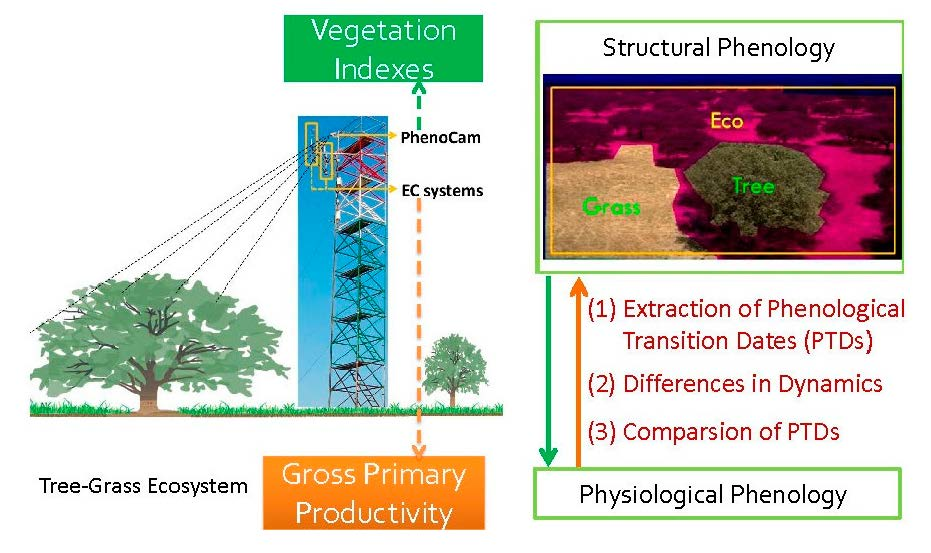
Moreover, the increasing number of sites with PhenoCam associated with EC flux measurements open interesting perspectives to evaluate: first, the consistency between PTDs derived from PhenoCam-based VIs and PTDs of ecosystem functioning (physiological phenology, i.e., [48]); second, the direct relationship between PhenoCam-based VIs and GPP. However, to our knowledge, only a few studies pay special attention to the differences between phenology of ecosystem structure and of ecosystem functioning and carbon fluxes [28,32].
In this study, our main objective is to evaluate the potential of PhenoCam to monitor phenology of seasonally dry Mediterranean tree–grass ecosystems. Specifically, the objectives are (1) to characterize structural and physiological phenology of tree–grass ecosystems and their main climatic drivers using PhenoCam and GPP derived from EC measurements; (2) to compare the PTDs and growing season length (GSL) derived from different PhenoCam-based VIs, and to evaluate their performance in tracking the PTDs and GSL derived from GPP.

2. Materials and Methods

2.1. Sites Description, Instrument Set-Up, and Data Sources

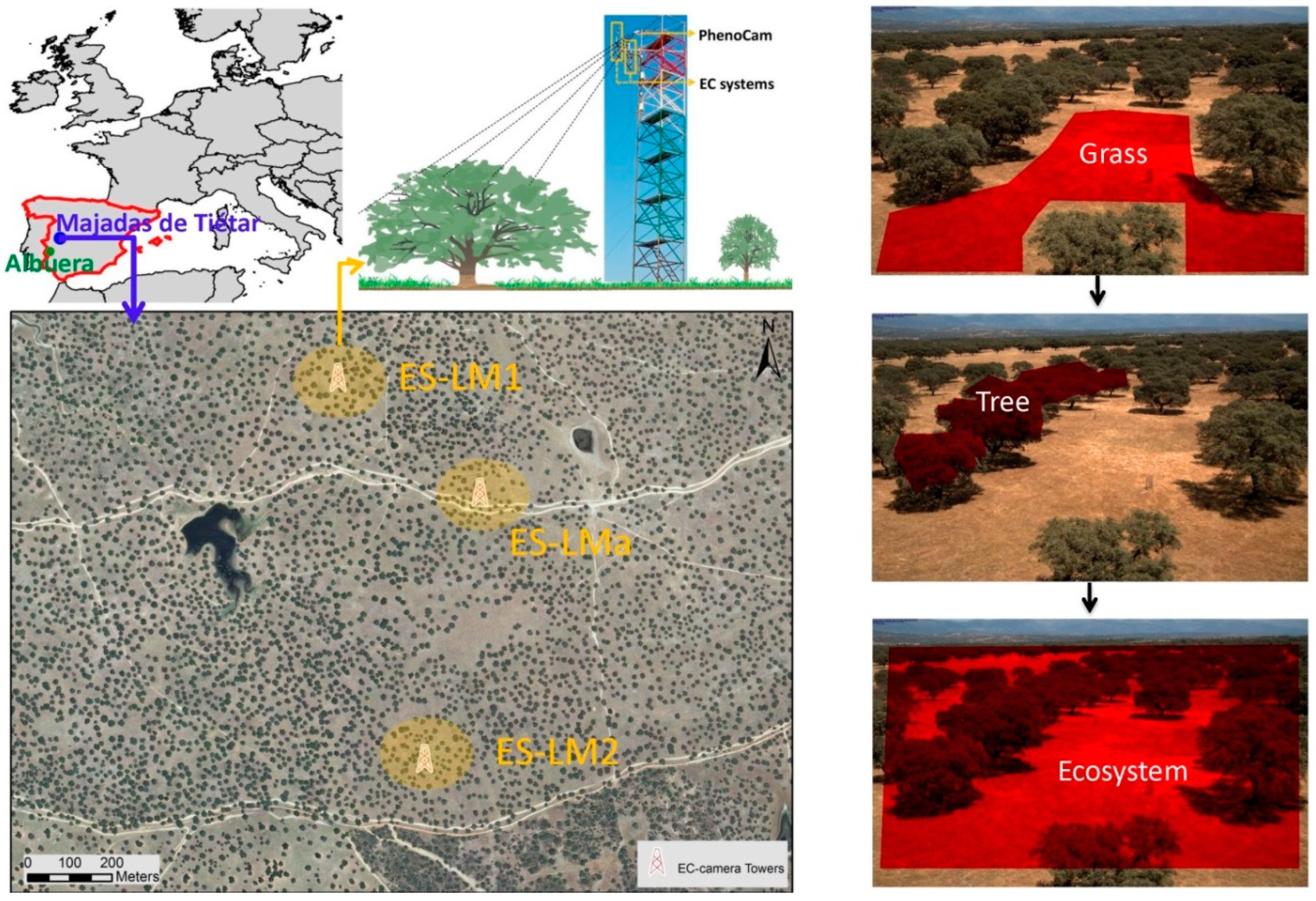
The sites used in this study are Mediterranean tree–grass ecosystems, composed predominantly of an herbaceous layer and low-density evergreen broadleaf oak trees (Quercus ilex; ~20 tree ha−1; Figure 1). Three sites are located approximately 500 m apart from each other in Majadas de Tiétar, Cáceres, Spain (39°56′24.68″N, 5°46′28.70″W), while one site is located in La Albuera, Spain (38°42′6.48″N, 6°47′9.24″W). The experimental sites in Majadas de Tiétar belong to a large-scale manipulation experiment, where the three areas of approximately 20 ha were manipulated with addition of nitrogen (FLUXNET ID ES-LM1), nitrogen and phosphorous (FLUXNET ID ES-LM2), and the last was kept as control (FLUXNET ID ES-LMa). The experimental site in the La Albuera (FLUXNET ID ES-Abr) is a natural ecosystem with no manipulation. In this study, we did not focus on the fertilization, but only on the evaluation of the effectiveness of different vegetation indexes to represent the ecosystem functions. The Majadas de Tiétar and La Albuera are characterized by a long-term annual mean air temperature of 16.7 ± 0.2 °C and 18.3 ± 1.5 °C, respectively; while mean annual rainfall is ca. 650 mm and 400 mm, respectively. The rain falls typically from November to May with a very dry summer [49].
In each site, an EC system was installed at 15 m of height to measure the carbon, water and energy fluxes (Section 2.2 for more details). The fluxes data are available from March 2014 in ES-LM1, ES-LM2, and ES-LMa; and from October 2015 for ES-Abr. Two broadband Decagon SRS (spectral reflectance sensor) sensors with a FOV of 36 degrees were installed on a rotating arm in each tower area. Downwelling irradiance and upwelling radiance at 650 nm (red spectral band) and 810 nm (near-infrared spectral band) were measured every 5 min for tree and grasses from 30 October 2015.
A NIR-enabled digital camera (Stardot NetCam 5MP), was mounted at the top of the EC tower (facing north) at each site. Images were collected every 30 min (from 10:00 to 14:30 UTC) as JPEG format. The camera settings were defined according to the “PhenoCam” protocol (https://phenocam.sr.unh.edu/webcam/tools/). Sequential red, blue, green (RGB) and RGB + NIR images were collected by the Stardot camera according to Petach et al., [
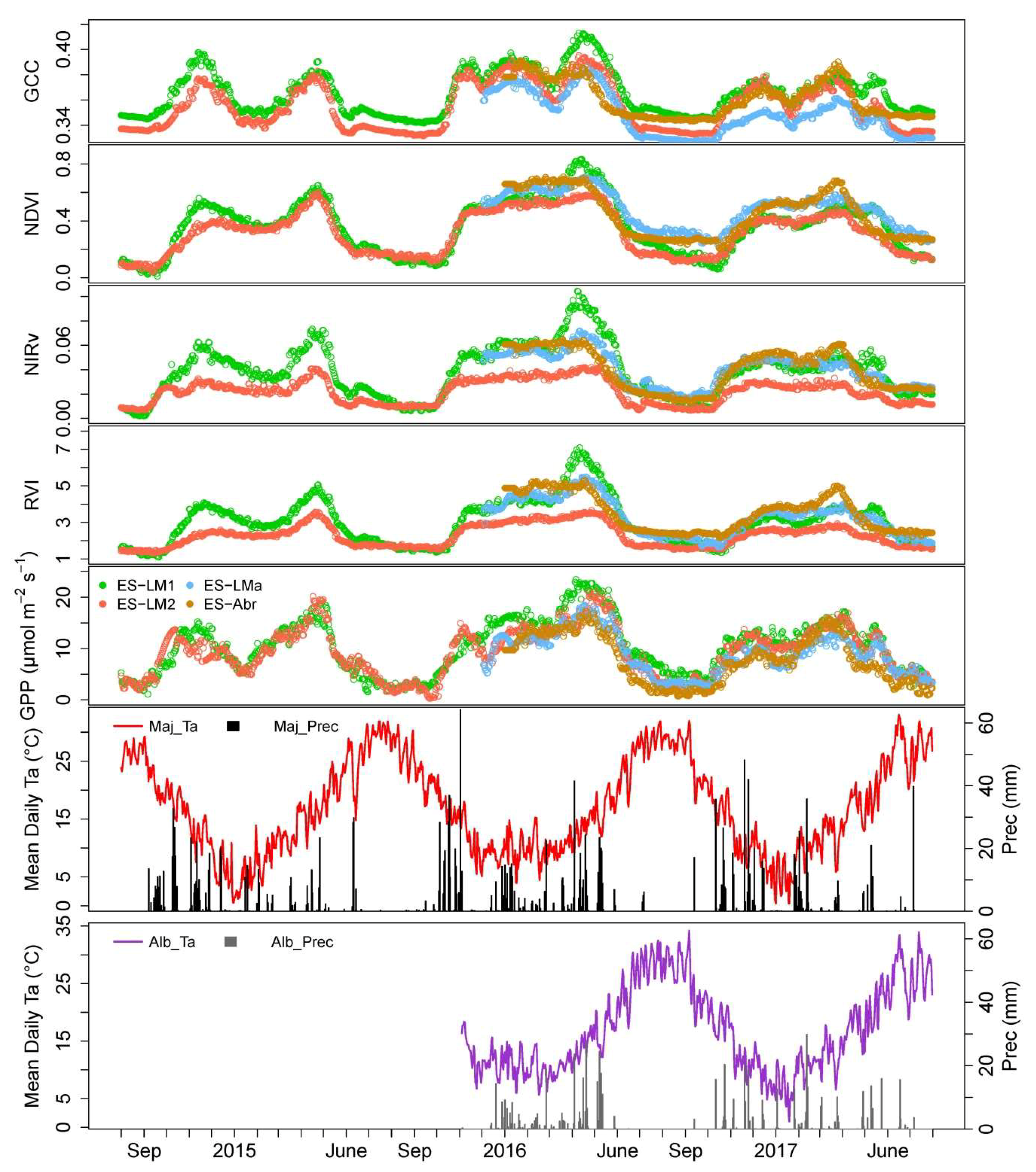
29]. FOVs of cameras in ES-LM1 and ES-LM2 were stable during the study period (from 1 August 2014 to 31 July 2017), whereas the FOV of ES-LMa was not constant and the camera experienced a white balance problem until 3 December 2015. At the ES-Abr site, images were available from 1 January 2016. Hence, RGB and RGB+NIR images were available for the analysis from 1 August 2014 to 31 July 2017 for ES-LM1 and ES-LM2; from 3 December 2015 to 31 July 2017 for the ES-LMa site; and from 1 January 2016 to 31 July 2017 for the ES-Abr site. This guarantees a total of 9 site-years for the following analysis.

2.2. EC Data Processing and Flux Partitioning to GPP

Each EC system consists of a three-dimensional sonic anemometer (R3-50, Gill LTD, Lymington UK) and an infrared gas analyzer (LI-7200, Licor Bioscience, Lincoln, NE, USA) to measure mixing ratios of CO2 and H2O. Additional vertical CO2 and H2O concentration profiles were measured at seven levels between the surface and the measurement height in the EC tower (0.1, 0.5, 1.0, 2.0, 5.0, 9.0, and 15 m above ground with a LI840, Licor Bioscience, Lincoln, NE, USA). Meteorological variables such as air temperature (Ta), wind speed (WS), relative humidity (RH), incoming global radiation (Rg), photosynthetically active radiation (PAR), and precipitation (Prec) were also measured at each site.
Raw EC data were collected at 20 Hz, and were then processed using EddyPro 6.2. The main processing procedures for CO2 fluxes included (1) coordinate rotation using planar fit method [50]; (2) CO2 time lag adjustments by covariance maximization in predefined windows; (3) spectral corrections performed for low and high pass-filtering effects according to Moncrieff et al. [51] and Moncrieff et al. [52]. The calculated flux for CO2 was then quality checked [53,54]. The net ecosystem exchange (NEE) flux was corrected by adding storage fluxes (integrated CO2 fluxes using seven levels of CO2 profiles when possible, otherwise using 1-point storage) to CO2 flux.
The u*-threshold, which was used as a criterion to discriminate low- and well-mixed eddies in the nighttime, was estimated for each year and tower individually (the median of u*-threshold ranges from 0.11 to 0.18 for ES-LM1, ES-LM2, and ES-LMa while 0.20–0.24 for ES-Abr) following Papale et al. [55].
The time series of NEE were gap filled using the marginal distribution sampling (MDS) method [56] which is based on lookup tables of temperature, global radiation, and water vapor pressure deficit (VPD) classes for short temporal windows i.e., 14 days. The gap-filled time series of NEE were then partitioned into GPP as described in Reichstein et al. [56]. In brief, the nighttime flux (Rg < 10 W/m2) of NEE (i.e., only respiration) is extrapolated from nighttime to daytime through a temperature response function, which is based on short term temperature sensitivities (for details see [56]). The u*-threshold, gap-filling, and partitioning was performed with the R package REddyproc [57].

2.3. Calculation of Vegetation Indexes from PhenoCam

Digital numbers (DNs) of each individual channel (RDN, GDN, BDN and NIRDN) were extracted from each photograph, and averaged over the different regions of interest (ROIs) (Figure 1). The overall brightness of each ROI (RGBDN) and the relative brightness of green channel, known also as green chromatic coordinates—GCC, were computed with Equations (1) and (2):
RGB DN = R DN + G DN + B DN  
GCC = G DN RGB DN  
CamNDVI was also computed in the different ROIs according to Petach et al. [29], using the algorithm implemented in the “phenopix” R package [34,36]:
CamNDVI = NIR DN R DN NIR DN + R DN ,
where NIRDN‘ and RDN’ are the adjusted exposure values of NIRDN and RDN, respectively. For a detailed calculation and the exposure adjustment formula, please refer to Petach et al. [29]. As the RDN’ and NIRDN’ are not direct measurements of reflectance, the CamNDVI values are not directly comparable to the NDVI from other data sources. Petach et al. [29] found a linear relationship between CamNDVI and the NDVI derived from the radiometric sensor (ASD FieldSpec 3) using the bands of 750 nm for the NIR and 605 nm for the red. They suggested using the linear regression coefficients to adjust the CamNDVI values for comparability with NDVI from radiometers [29,34].
Therefore, we applied the method suggested by Petach et al. [29] and Filippa et al. [34] to rescale CamNDVI using the NDVI derived from the Decagon SRS (VIs was calculated and averaged over a 30 min period to be consistent with VIs from PhenoCam). The coefficients and statistics of the linear regression used to compute the scaling factors are shown in Table 1. In the following only the rescaled CamNDVI values are used and presented.
Likewise, the CamNIRv and CamRVI were also calculated with adopting Equations (4) and (5) which refer to Badgley et al. [41] and Chen [42], respectively.
CamNIRv = CamNDVI × NIR DN ,
CamRVI = NIR DN R DN ,
where NIRDN′ and RDN′ are the adjusted exposure values like Equation (3). A similar approach used for the CamNDVI was used to compute CamNIRv and CamRVI: SRS-based NIRv and RVI were used to adjust the CamNIRv and CamRVI in order to make them comparable with the data derived from other sources (Table 1).
The analysis was conducted on various ROIs as depicted in Figure 1: we selected ROIs with only trees, grass, and both (hereafter referred as Tree, Grass, and Eco ROI, respectively). The different sites have different tree/grass proportions in the camera FOVs, as only one direction of ecosystems could be captured from the PhenoCam. However, the fractional tree canopy covers were consistent (~0.20) in the four sites by referring to field surveys and the classification analysis using airborne hyperspectral imagery [58,59]. The analysis of each footprint for each EC tower also indicates GPP is contributed from ~20% tree canopy and ~80% grasses [59]. In order to reduce the bias introduced by the different ratios of tree/grass in the images and camera FOV, which has to do with logistical constrains during the camera installation, the ecosystem VIs (GCC, CamNDVI, CamNIRv, CamRVI) were computed by using the weighted average of the VIs derived from Grass ROIs of 0.8 and Tree ROIs of 0.2.

2.4. Data Filtering and to Compute Daily VIs and GPP

After computing the half-hourly VIs (GCC, CamNDVI, CamNIRv, CamRVI) at ecosystem scale, we applied a series of steps to derive robust time series of daily VIs:
  • We discarded VIs measured with PAR below 600 µmol m−2 s−1. This procedure was used, on one hand, to filter out the VI values measured during adverse meteorological conditions (i.e., rainy, foggy, or overcast half-hours [34,48]), and on the other hand, Petach et al. [29] suggests to apply a threshold on PAR to reduce the variability of CamNDVI due to changes in illumination conditions. Here, we selected a more conservative threshold than Petach et al. [29].
  • A max.density filter method was developed to filter and retrieve daily VIs. We constructed the probability density function (PDF) of VIs in 3-day moving windows (30 observations), and assigned the value that has highest probability density as the filtered daily value. We did not apply the widely used max method [22,36], which uses the 90th percentile of the VIs value from a 3-day moving window as the filtered daily value. This is because the variability of NIRDN is larger compared to other channels (i.e., RDN, GDN, BDN) in the PhenoCam, which would result in large variability of VIs (i.e., CamNDVI, CamNIRv and CamRVI) that is especially obvious for Mediterranean ecosystems compared to other ecosystems (some comparison using data retrieved from [34], results are not shown in this study). Hence, we chose to apply the max.density filter to retrieve time series of VIs with less variability, which were not always retrieved by applying max filter in our study. We used an example to demonstrate the better filter performance of max.density compare to max filter methods in our study (Figure A1).
  • Daily VIs were gap-filled using the Singular Spectrum Analysis (SSA) method implemented in the “spectral.methods” R package [60].
  • Similar to the processing of VIs, the daily GPP was derived from half-hourly data following the step (2) and step (3).

2.5. Phenological Transition Dates (PTDs) Extraction

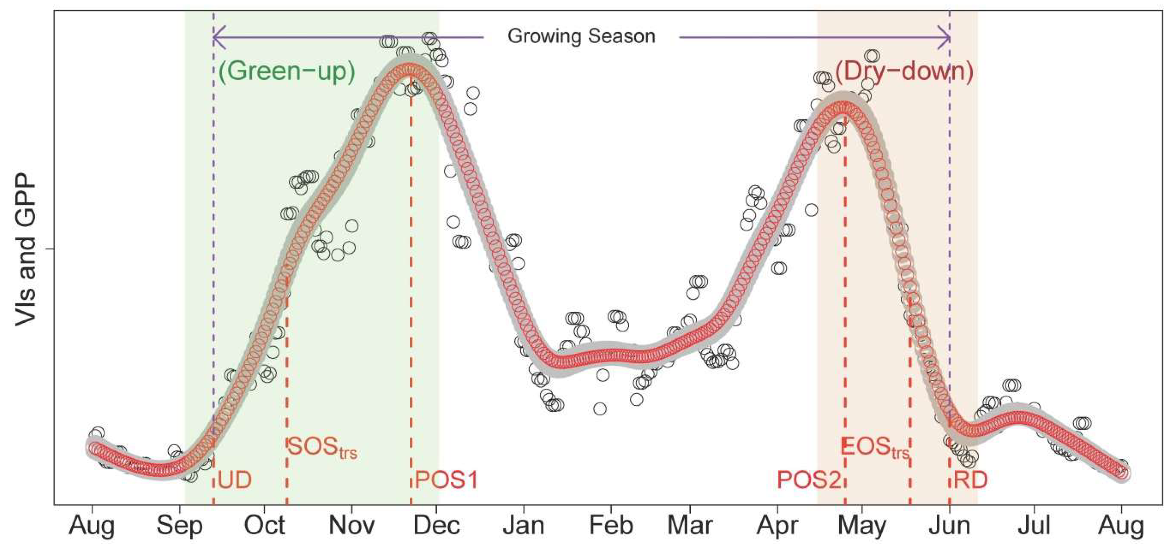
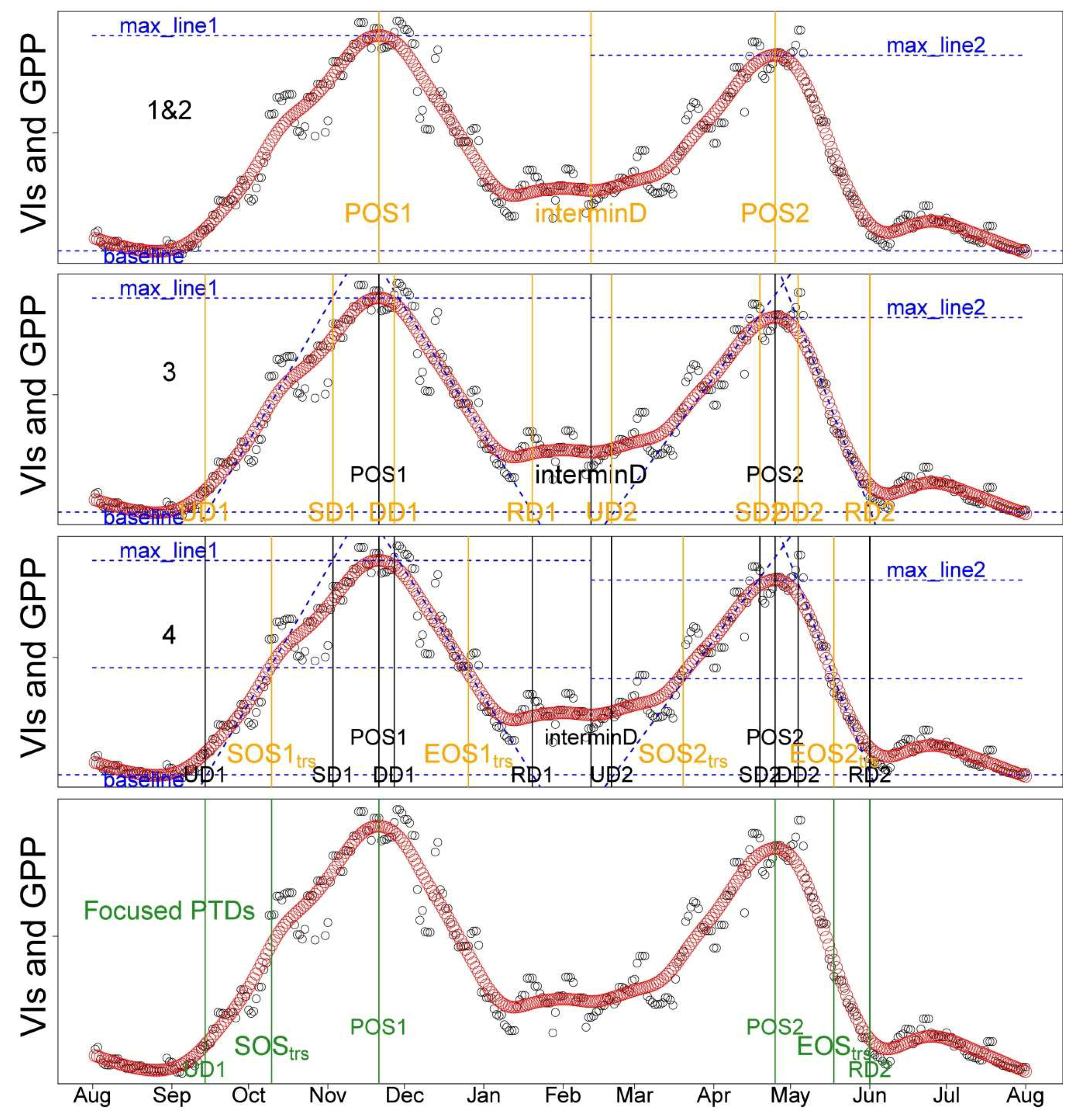
The Mediterranean climate is characterized by rainy late autumn–winters, and warm dry summers. Typically, the studied tree–grass ecosystems are dry and covered with senescent grasses in summer, while they increase in greenness in the late autumn (after the onset of the rainy season) and spring. Considering the characteristics of the phenological cycle described above, we decided to conduct the analysis using the concept of “hydrological years”, which is, here, defined from 1 August to 31 July (Figure 2).
In this study, we developed a PTD extraction method for PhenoCam-based VIs in seasonally dry tree–grass ecosystems. The methodology of PTDs extraction is composed by the following steps:
  • Data were smoothed using the spline method [20,36]; PTDs were extracted using the derivatives of smoothed seasonal cycle [61] and applying thresholds (i.e., 50%) of amplitude of VIs [
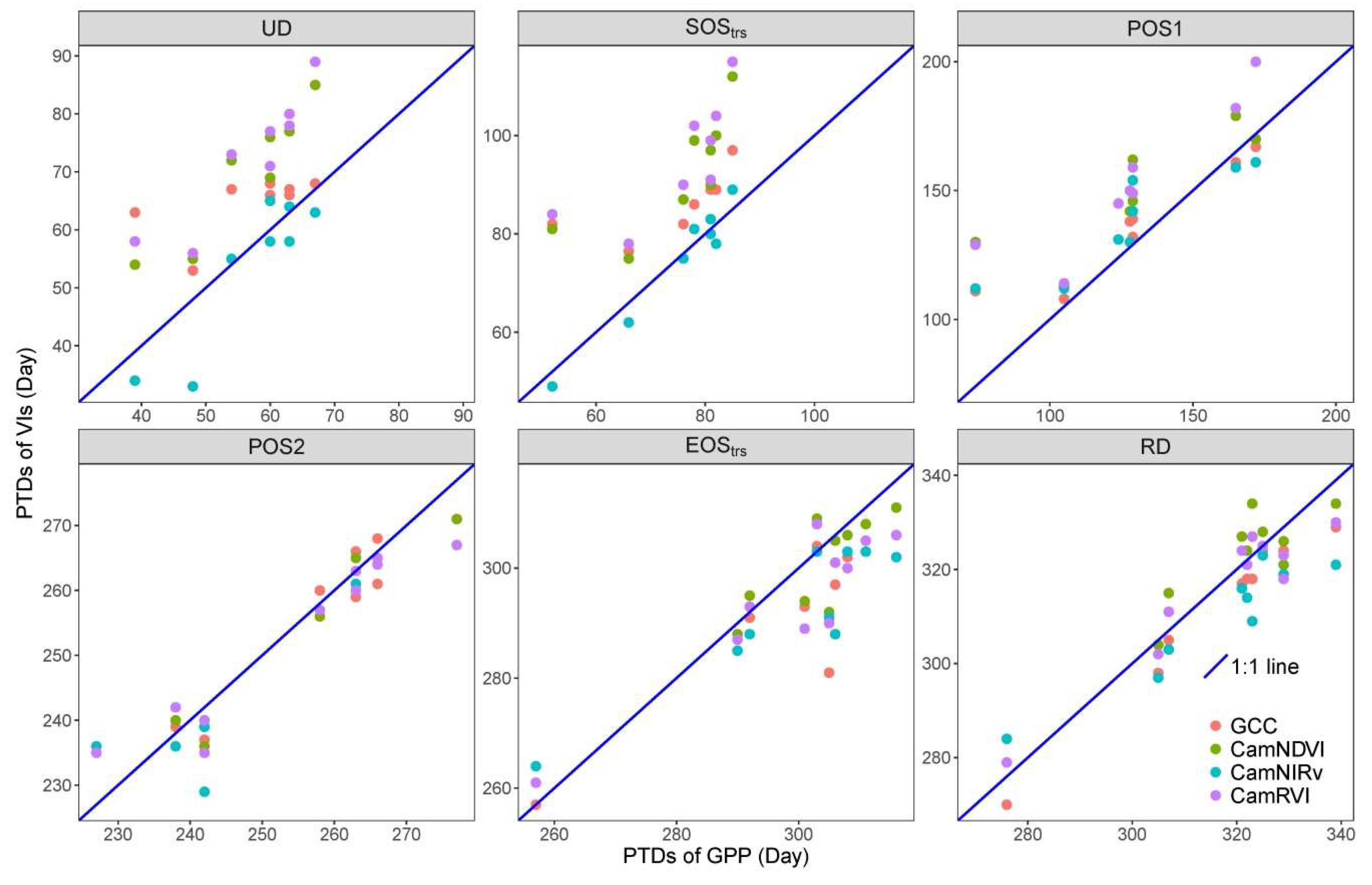
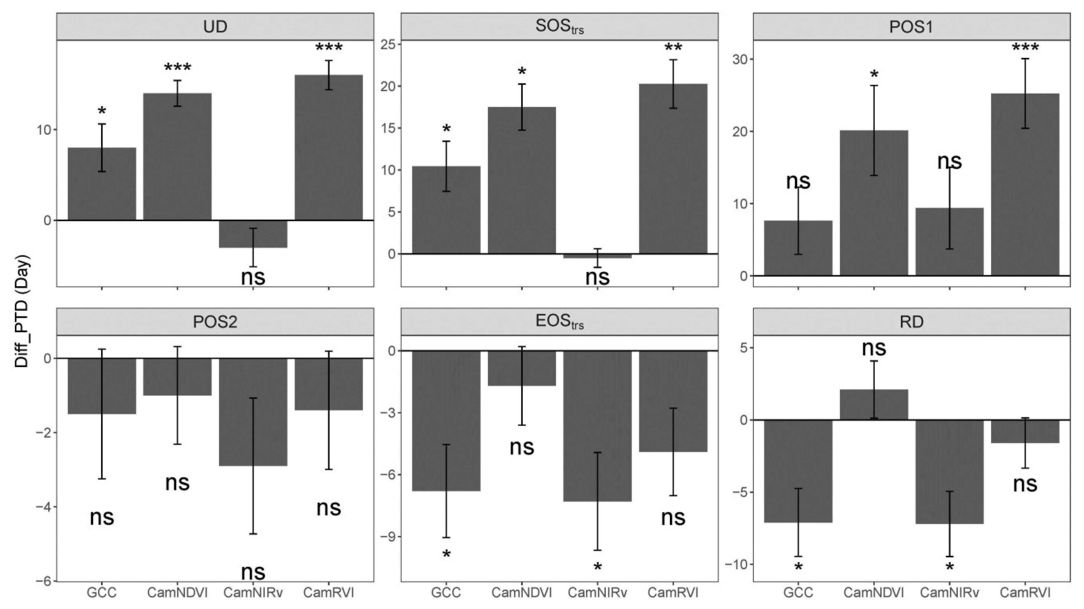
62]. As the start and end of the season are extremely important to characterize the phenology, we defined two sets of PTDs in the start (UD, SOStrs; Table 2) and end of season (RD, EOStrs; Table 2) for intercomparison and better characterizing the phenology. These two sets of PTDs are derived based on different perception and methodology. UD and RD are retrieved as the intersection dates between steepest slope and minimum value in the Green-up and Dry-down periods, respectively [61]. In contrast, SOStrs and EOStrs are retrieved by using the thresholds of 50% amplitude [62]; i.e., they are defined when 50% of amplitudes are reached in the Green-up and Dry-down periods, respectively. Other extracted PTDs and the phenological periods analyzed in this study were summarized in Figure 2 and Table 2. The detailed procedures and corresponding code related to the extraction of PTDs are provided in Appendix B.
  • Uncertainty of extracted PTDs was assessed by extracting PTDs repeatedly (100 times) from an ensemble of time series constructed by summing original data and random noise as described by Filippa et al. [36].

2.6. Statistical Analysis

All the statistical analyses were conducted with the R 3.4.3 programming language [63]. The differences among PTDs extracted from the different datasets (GCC, CamNDVI, CamNIRv, CamRVI, and GPP) were evaluated using the mean absolute error (MAE) and root mean squared error (RMSE) (Equations (6) and (7)):
MAE = 1 n i = 1 n | y i y i | ( day ) ,
RMSE = 1 n i = 1 n ( y i y i ) 2 ( day ) ,
where yi’ and yi were the PTD dates extracted from two different datasets. Wilcoxon signed-rank tests were used to test for statistically significant differences between each paired PTDs from the different datasets given that were not normally distributed, while paired Student’s t tests were used when PTDs were normally distributed.
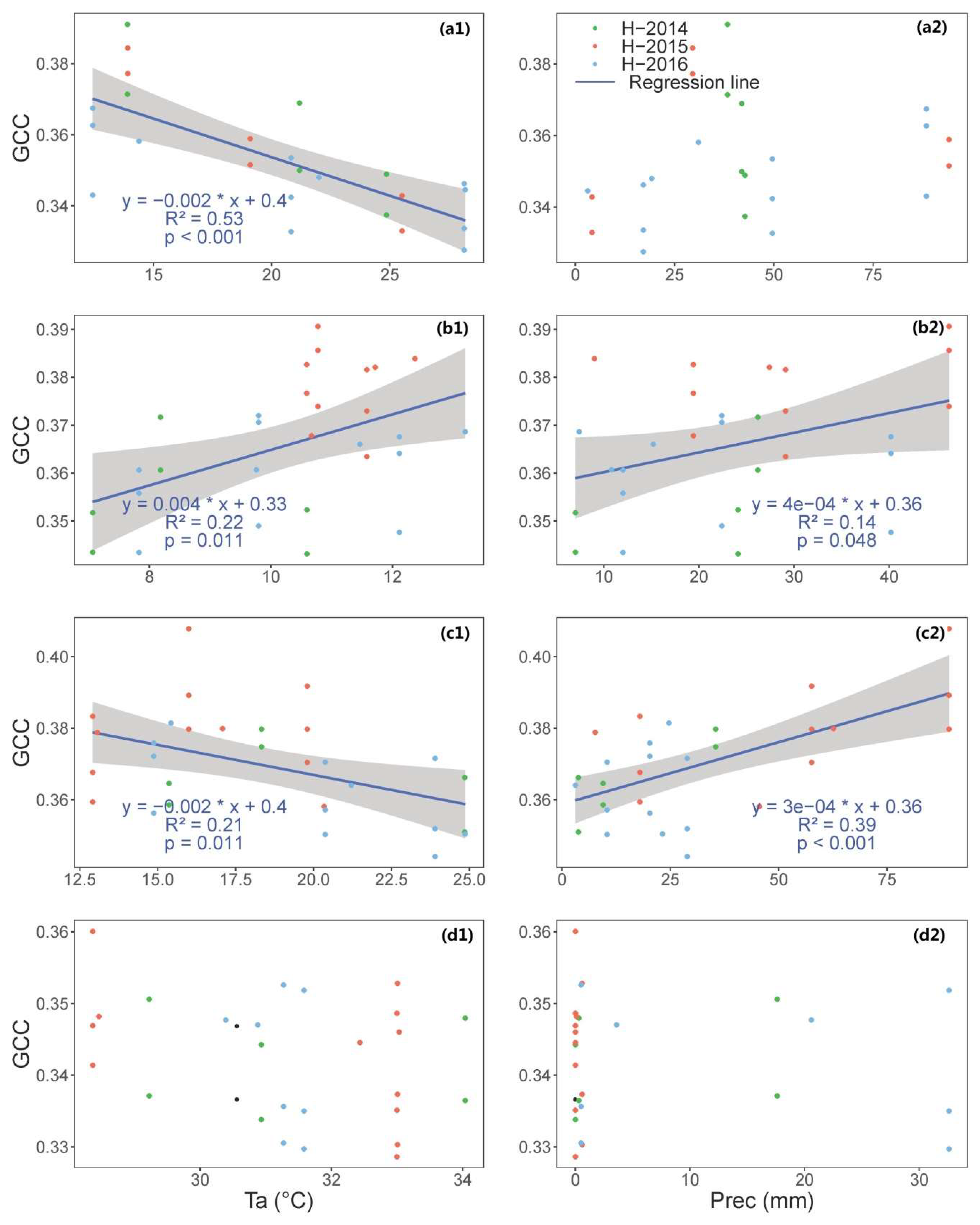
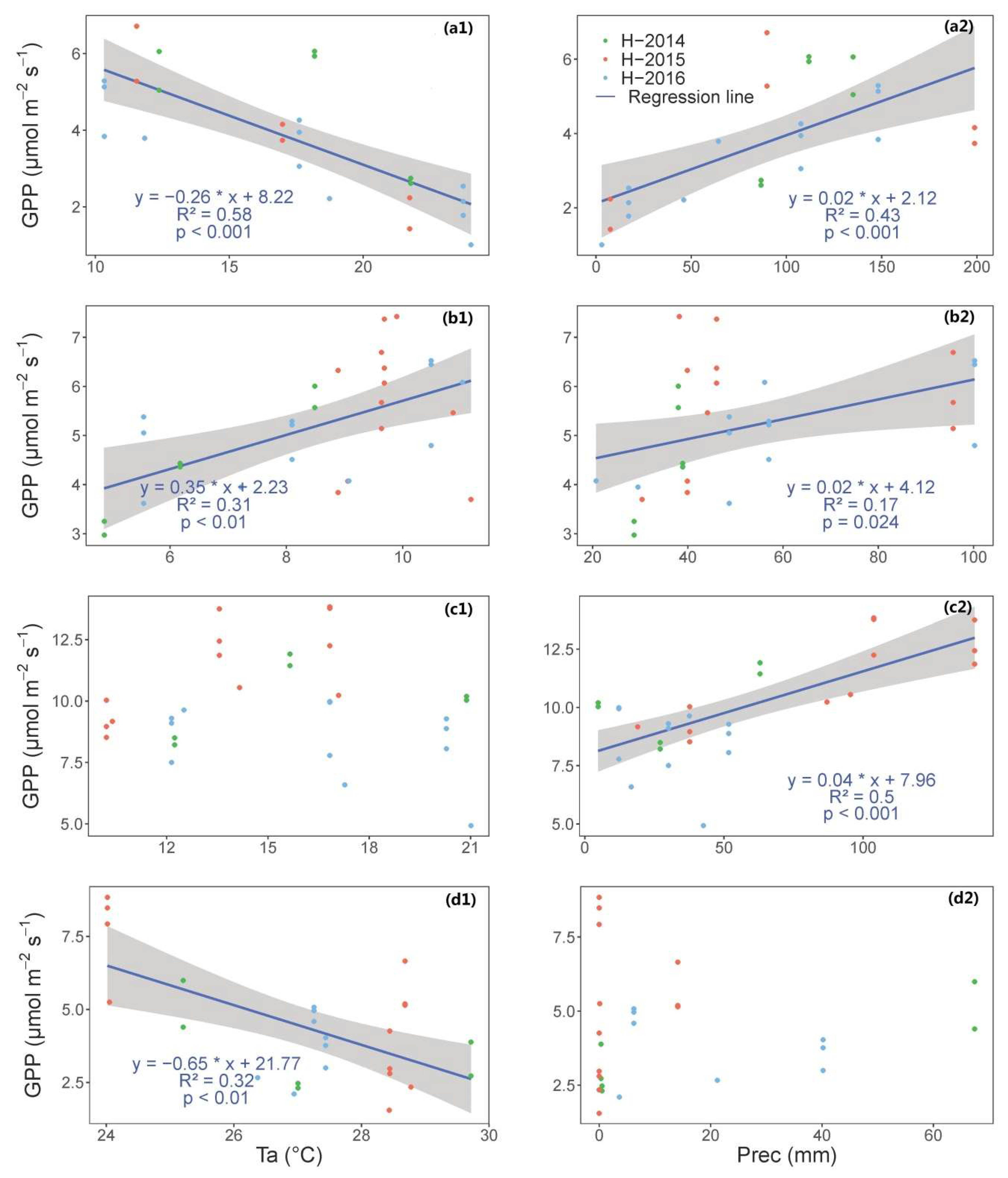
The linear regressions were conducted between time series of VIs and GPP, or between meteorological variables and GPP using ordinary least squares regression (OLS). However, the linear regression between PTDs and GSL extracted from different VIs and GPP was conducted using major axis regression (R package “lmodel2”) to account for errors of similar magnitude in the y and x axis.

3. Results

3.1. Time Series of VIs (GCC, CamNDVI, CamNIRv, CamRVI), GPP, and Their Relationship with Meteorological Conditions

The seasonal variation of VIs and GPP, as well as their correlations, are shown in Figure 3 and Table 3, respectively. In general, all VIs have distinct seasonal variations and are consistent with the temporal variability of GPP (Figure 3 and Table 3). At four sites, all VIs have significant and good correlation with GPP (Pearson’s correlation coefficient: r ≥0.85; Table 3). The determination coefficients (R2) of linear regression between VIs and GPP also range from 0.72 to 0.87, in particular, with slightly higher R2 for CamNDVI and CamRVI. However, VIs have distinct discrepancies on variation range. For instance, the GCC of our sites ranges 0.32–0.42, while the CamRVI could vary between 1 and 7.
Distinct interannual variability of VIs and GPP are also observed at the four sites (Figure 3). The time series (GCC, CamNDVI, CamNIRv, CamRVI, and GPP) have an obvious “two-humped” shape in the hydrological year 2014 (Hydro-2014: 1 August 2014–31 July 2015) and hydrological year 2016 (Hydro-2016: 1 August 2016–31 July 2017), while the shape is not clear in the time series for the hydrological year 2015 (Hydro-2015: 1 August 2015–31 July 2016; Figure 3). The absence of the two-humped shape in Hydro-2015 coincides with the warmer mean air temperature (Ta) observed in winter 2015 (9.4 ± 2.4 °C) and lower Ta in spring 2016 (13.5 ± 3.5 °C) compared to Hydro-2014 (6.4 ± 3.3 °C and 16.3 ± 4.3 °C, respectively) and Hydro-2016 (8.0 ± 3.4 °C and 16.4 ± 4.6 °C, respectively; Table A1 and Figure 4). The onset of growing season in each hydrological year clearly followed the onset of the rainy season, confirming that autumn phenology in these ecosystems is driven by precipitation (Figure 3). Larger precipitation (281.7 mm) in the spring of Hydro-2015 also leads to higher GPP compared to Hydro-2014 (94.9 mm) and Hydro-2016 (94.0 mm; Figure 4 and Table A1), both characterized by less than half of the precipitation compared to Hydro-2015.

3.2. Comparison of Phenological Transition Dates (PTDs) Derived from Different VIs

The comparison of PTDs extracted from different VIs is shown in Figure 5. Generally, the PTDs derived from the different VIs show smaller difference between each other at Dry-down periods (POS2, EOStrs, RD) compared to the Green-up periods (UD, SOStrs, POS1). Specifically, PTDs derived from GCC have the smallest differences with PTDs derived from CamNIRv, while they are significantly advanced from the ones from CamNDVI at the Dry-down period (Figure 5). During Green-up periods, the PTDs derived from GCC are more advanced than the ones from CamNDVI and CamRVI, while they are also delayed compared to PTDs extracted from CamNIRv. By contrast, the PTDs derived from CamNDVI are all more delayed than the PTDs from CamNIRv, in particular, with more than 10 days difference at Green-up period. However, they have small differences compared to the PTDs extracted from CamRVI (<5 days), but they are significantly advanced at Green-up and delayed at Dry-down periods, respectively. Similar to GCC, the PTDs derived from CamNIRv are also advanced than the ones derived from CamRVI with large difference at Green-up period (>15 days).

3.3. Comparison of Phneological Transition Dates (PTDs) Derived from VIs and GPP

The comparison of PTDs derived from different VIs and GPP is shown in Figure 6 and Figure 7. The PTDs derived from VIs for the Green-up period (UD, SOStrs, and POS1), with the exception of CamNIRv, are systematically delayed from the ones derived from GPP (Figure 6). By contrast, the PTDs extracted from the VIs have a good agreement with the PTDs extracted from the GPP in the Dry-down period (POS2, EOStrs, RD). The difference between PTDs extracted from VIs and GPP ranges within 10 days in the Dry-down period. By contrast, their difference ranges from 8–25 days for the Green-up period, with the only exception of CamNIRv and GPP, which show a smaller difference (Figure 7 panel UD and EOStrs).
Specifically, the PTDs derived from CamNIRv at the Green-up period and the ones derived from CamNDVI at the Dry-down period have no significant difference compared to the ones derived from GPP, respectively (Table 4). The PTDs extracted from CamNIRv and GCC have smaller differences (9.4 and 7.0 days, respectively) with the ones derived from GPP in the Green-up period, while they have larger difference with the PTDs derived from GPP compared to CamNDVI (difference of 4.6 days) and CamRVI (difference of 5.0 days) in the Dry-down period (Table 4 and Table A2).
The results show that POS1 derived from VIs have a large difference with the POS1 derived from GPP especially for CamNDVI and CamRVI (>20 days). All the POS2 derived from VIs have no statistically significant difference with the ones extracted from GPP, with the difference between VIs and GPP ranging within 5 days (Figure 7).

3.4. Comparison of Growing Season Length (GSL)-Derived VIs and GPP

The growing season length (GSL: defined as the difference between PTDs of RD and UD) derived from GPP shows no statistically significant difference with GSL calculated from CamNIRv (Figure 8). By contrast, GSLs derived from GCC, CamNDVI, and CamRVI is statistically significantly different from GSL derived from GPP with mean absolute error (MAE) of 12.2, 10, and 15.5 days, respectively (Figure A4). We also compare the GSLs derived from GPP and VIs with the GSL defined as the difference between EOStrs and SOStrs, which is widely used in the remote sensing field. The results (Figure A5) also agree with the above results.
In general, the GSL calculated from GPP is larger than the ones derived from the VIs (Figure 8 and Figure A4). Most of GSLs range from 240 to 270 days, with the exception of GSL derived from ES-Abr sites, which is the driest site among the four studied (Figure A4). GSLs derived from different VIs have good correlation between each other (r >0.8; Figure A4). Specifically, GSL derived from GCC has the least difference (MAE: 4.8 days) between the ones derived from CamNDVI. GSL derived from CamNDVI and CamRVI has a difference of 5.8 days. Contrastively, GSL derived from GCC, CamNDVI and CamRVI has a relatively high difference (>8 days) between the GSL derived from the CamNIRv (Figure A4).

4. Discussion

4.1. Characterizing Variatoin and Drivers of Structural and Physiological Phenology

Here, we discuss and characterize the phenology of a seasonally dry Mediterranean tree–grass ecosystems using high temporal resolution of VIs (i.e., daily) derived from PhenoCam and GPP from EC towers. We found large seasonal variations in both PhenoCam-based VIs (structure) and GPP (physiology). In general, seasonal variations in PhenoCam VIs were in phase with those of GPP (Figure 3 and Table 3). We argue that seasonal variations in VIs and GPP are driven by the herbaceous layer, which dominates the ecosystem dynamics in our study sites [59]. Our sites are characterized by relatively sparse evergreen broadleaf trees (~20%) and a larger fraction of annual grasses [59]. Foliage amount in evergreen tree species remain relatively constant throughout the year, and they can utilize their vast root system to access the water deep within the soil [64,65,66]. By contrast, grasses are highly responsive to rainfall variations in rainy seasons as they tend to use water and nutrients in topsoil with dense shallow roots [11,67]. The yellowing grasses in senescence lose their vigor during the dry and hot summer. Being that the VIs derived from the tree are relatively constant during the year, grasses contribute a large proportion of VIs (Figure A6) and GPP in rainy seasons, but trees contribute more during dry periods [49].
Meteorology plays an important role in governing seasonal variation of VI and GPP (Figure A2 and Figure A3), though the role and importance of water availability and temperature varies across seasons (phenological stages). In autumn, after the dry season, the onset of greenness and GPP is initiated by the onset of the rainy season (Figure 3). In winter, water is not a limiting factor, due to the typical ample precipitation in late autumn and early winter. On the other hand, we observed that winter temperature is an important limiting factor of plant photosynthetic activity [68] (Figure 4). In spring, with the increase in incoming radiation and day length, temperature, and associated increase in atmospheric evaporative demand (i.e., VPD), we found precipitation strongly correlated with both GCC and GPP (Figure 4); this is consistent with previous findings over Mediterranean ecosystems [69,70,71]. In summer, which is the dry season, precipitation triggers an abrupt increase of VIs and GPP, as observed after the heavy rain that occurred in the June-2016 and July-2017 (Figure 3). The large rain pulses caused a decrease in temperature and an increase in water availability, further contributing to the regrowth of plants, in particular, at the early stage of the dry season (Figure 3). On the annual scale, growing season lengths (GSLs) derived from ES-Abr tower are significantly shorter than the GSL derived from the other sites in Majadas de Tiétar (i.e., ES-LM1, ES-LM2, and ES-LMa; Figure 8), which might be attributed to a lower water availability at the ES-Abr tower more than the other sites. In fact, ES-Abr is characterized by about 200 mm of rain less than the sites located in Majadas de Tiétar.
In this study, we also observed the important influence of both structural (VIs) and physiological phenology (i.e., GPP) exerted by extreme climate events. There was an extremely warm winter followed by wetter than average spring in Hydro-2015 [72], which led to a significant impact on both VIs and GPP over our study sites (Figure 3 and Table A1). The growth and productivity, in particular of the herbaceous layer, was stimulated by high temperature and concomitant water availability in the winter of Hydro-2015, while lower temperature and higher precipitation (~2 times more than Hydro-2014 and Hydro-2016) slow down the growth of plants in the spring (Figure 4 and Table A1). This reduced the difference of VIs and GPP between winter and spring, and further caused the observed disappearance of the typical “two-humped” shape of Mediterranean ecosystems (Figure 3). Moreover, the warm spell in winter contributed to an extremely high GPP and greenness (Red dots in Figure 4) that substantially contributed to the annual total GPP [72]. These results point towards the important, and often neglected, contribution of winter periods to interannual variability of GPP and phenology in the Mediterranean ecosystems. In this study, we did not focus on the effects of the fertilization on PTDs, productivity, and growth; rather, we focused on the development of the framework to characterize phenology in seasonally dry Mediterranean ecosystems using PhenoCams. Therefore, further analysis will focus on better understanding the sensitivity of structural and physiological phenology to nutrient availability, meteorological drivers and rain pulses by means of model–data integration (e.g., [7,20,73,74]).

4.2. Utilizing Different PhenoCam-Based VIs to Represent Structural Phenology

We found distinct differences in the PTDs extracted from GCC and CamNDVI, two widely used indexes from PhenoCam (Figure 5). Overall, the PTDs derived from the GCC anticipate the ones derived from the CamNDVI, which is in line with previous studies [28,29,34,75]. In the Green-up period (UD, SOStrs, and POS1), changes in CamNDVI are more gradual than the changes in GCC (Figure 5) [29], which is likely due to the fact that GCC is more sensitive to color changes of leaves under low value of leaf area index (LAI; LAI < 2 [28]). Wingate et al. [28] found that the initial increase of GCC during the early growing season is caused by the rapid changes in leaf area and leaf chlorophyll content (Chl). With the increase of foliar biomass associated with shoot elongation and the formation of new leaves [28,76] after the early growing season, CamNDVI, which is more sensitive to the changes of canopy structure, increases continuously while GCC has no substantial changes [34]. Previous studies also found that GCC becomes saturated when nitrogen content or Chl only reaches half of the maximum value at Green-up periods [35,75]. By contrast, NDVI continues to increase with the maturation of leaves [77] and the increase of LAI in the canopy [35,75]. This likely explains why there is a big difference in the timing of the first peak (POS1) of greenness between GCC and CamNDVI (Figure 5).
Similar to the Green-up period, during the Dry-down period, GCC is more sensitive to color changes in leaves from green to yellow, while CamNDVI is a better proxy for variation of LAI and biomass [28,29,34]. During the Dry-down, the total green LAI of grasses start decreasing, but there is a large amount of dry and senescent biomass presented in the top canopy [78]. As such, we observed an earlier decline of GCC than CamNDVI during the Dry-down period [34] (Figure 5). The complementary information provided by GCC and CamNDVI point towards the need of using both indices to monitor structural changes of the canopy [29,34], as well as the need for investigating different VIs that can be computed from PhenoCam.
To our knowledge, this study is the first attempt to compute the CamNIRv and CamRVI, and to compare them with the more widely used GCC or CamNDVI [34,41]. There is a systematic difference in PTDs extracted from CamNIRv as compared to those derived from other VIs, particularly for PTDs from the Green-up period. The PTDs derived from CamRVI tend to be later than those from CamNDVI and other VIs. This result is in agreement with Viña et al. [79], which also showed that satellite-based NDVI increases faster than RVI with the increase of LAI in maize and soybean fields.
Our results confirmed that PhenoCam-based VIs provide complementary information that can be used to monitor phenology of structure (biomass, greenness). The systematic differences observed between VIs are consistent with results reported in the literature [34,75] and obtained with spectroradiometers [29,34] or satellites [80]. Future studies are needed to analyze the systematic differences between PhenoCam-based VIs (e.g., the comparison between NIRv and other VIs). For instance, studies that combine physiological measurements and plant traits collected in the field with PhenoCam data [75,77], in parallel with the use of radiative transfer models (e.g., Wingate et al., [28]) can provide valuable information to better understand the difference between VIs and different aspects of vegetation phenology.

4.3. Combing Different PhenoCam-Based VIs to Represent Physiological Phenology

The relationship of VIs derived from PhenoCam imagery with ecosystem-scale carbon fluxes in semi-arid systems is recently receiving more attention. However, to our knowledge, previous studies focused mainly on the relationship between GPP and GCC, and here, we move forward to include other potential VIs that can be derived from PhenoCams. We observed varying performance among PhenoCam-based VIs in tracking physiological phenology as measured by GPP. During Green-up period, the PTDs derived from CamNIRv agreed the best with the PTDs derived from GPP (Figure 6 and Table 4). Apart from CamNIRv, the UD and SOStrs derived from the GCC, CamNDVI, and CamRVI are statistically delayed more than the ones derived from the GPP (Figure 7). Our results about the differences between GPP and GCC are contrasting to previous studies [20,32,75], which mostly focused on temperate deciduous forests, evergreen needleleaf forests or grasslands, while the relationship between GCC and GPP is comparable to a study focused on a grassland understory of a “open forest savanna” in Australia [30]. One possible explanation for the discrepancy between previous studies [20,32,75] and this study, can be related to the patterns of re-greening of the vegetation in autumn after the onset of the rainy season. At the beginning of the Green-up period, the canopy of the grass is characterized by a relevant amount of dry biomass (~38% senescent grasses as measured between October to November 2014–2015). Therefore, the new emerging grasses contribute to the photosynthetic activities, but not so much to the measureable greenness. For this reason, the GPP increases systematically earlier than GCC. However, there is evidence in the literature that this systematic delay is dependent on the greening patterns and mechanisms of vegetation phenology, therefore, it is vegetation type-dependent [20,32,75].
During the Dry-down period, the PTDs derived from CamNDVI are closer to the ones derived from GPP. The PTDs of EOStrs, and RD derived from GCC and CamNIRv are more advanced than the ones derived from GPP. Dry biomass starts to accumulate in the senescent period at the top of the grass canopy with still a certain amount of living biomass at the bottom. As mentioned above, GCC is sensitive to the changes of color [28,29,34,75], hence, PTDs derived from GCC are anticipated to advance more than the PTDs derived from GPP at Dry-down period. However, more investigations are needed to explain why CamNIRv is also more advanced than GPP at the Dry-Down period. By contrast, PTDs derived from CamNDVI and CamRVI have no statistically significant differences compared to the ones from GPP, which implies the potential to use CamNDVI or CamRVI to represent GPP in the Dry-down period.
For the timing of max structural and physiological phenology, we did not observe the systematic differences between PhenoCam-based VIs and GPP for the POS1 (Figure 7). However, the POS1 in our study is not comparable to the timing of the maximum value in other studies, as the POS1 in our study is in the winter time, while others are in the late spring or summer [32,75]. By contrast, the POS2 extracted from GPP is delayed compared to the POS2 extracted from VIs during the spring period (Figure 7), which agrees with previous studies [32,75].
As a key factor controlling net uptake of carbon dioxide [81,82], accurate estimates of GSL has rendered substantial interest, since it has distinct impacts on ecosystem function [83]. In this study, we also study the GSL as extracted from GPP and PhenoCam-based VIs. GSL derived from CamNIRv is most representative of the GSL derived from GPP (Figure 8, Figure A4 and Figure A5). NIRv is claimed to explain a large fraction of the variance of GPP, and has better representation than NDVI on monthly to annual time scales [41]. However, from our study, the CamNDVI better tracks the PTDs of GPP more than CamNIRv on the Drying-down period (Figure 7), which makes the GSL derived from the CamNDVI also close to GSL derived from GPP, though with a larger error compared to CamNIRv. Yang et al. [35] reported high correlation between physiological properties (e.g., leaf nitrogen content, leaf chlorophyll content) and CamNDVI, which implies CamNDVI could potentially track the GPP well.
In summary, NIR-enabled PhenoCam-based VIs (e.g., CamNDVI and CamNIRv) can improve the performance of PhenoCam to represent physiological phenology (i.e., variability of PTDs and GSL as derived from GPP). Compared to conventional PhenoCam (only with blue, green, and red channels), NIR-enabled PhenoCam-based VIs take advantage of the fact that green vegetation reflects more NIR than visible light, which makes them more relevant to monitor variation in biomass and seasonal variability in photosynthetic capacity [84]. More studies investigating other PhenoCam vegetation indices are needed, for instance NIRv and 2-band enhanced vegetation index (EVI2; EVI computed without blue band) could be complementary indexes to be applied to track GPP in future, as both indexes are reported to have a good relationship with GPP [41,85,86] and could be computed with two bands (Red and NIR).Our results confirmed that it is promising to utilize the NIR-enabled PhenoCam as a complementary and cost-effective way to characterize GPP, biomass, and phenology. In this study, we mainly focused on seasonal variability (PTDs and GSL) but at shorter time scales; it is still unclear how the different PhenoCam-based VIs presented in this study fully present the variability of GPP. For instance, some VIs could not accurately reflect the variation of GPP during short-term changes of weather conditions, like sudden warm spells or droughts, as pointed out in other studies [32,87]. Hence, we strongly suggest using multiple VIs to better characterize the GPP together with additional ancillary measurements, such as meteorology and leaf traits.

5. Conclusions

In this study, we assessed the potential to jointly use near-infrared-enabled digital repeat photography and eddy covariance data for monitoring structural and physiological phenology in seasonally dry Mediterranean tree–grass ecosystems. We analyzed 9 site-years using four PhenoCam-based vegetation indices (GCC, CamNDVI, CamNIRv, and CamRVI) and GPP, and we compared the phenological transition dates (PTDs) and growing season length (GSL) derived from the different data streams.
We show that, in Mediterranean tree–grass ecosystem, meteorology plays an important role in governing seasonal variation of vegetation indices and GPP, though the importance of water availability and temperature vary across seasons.
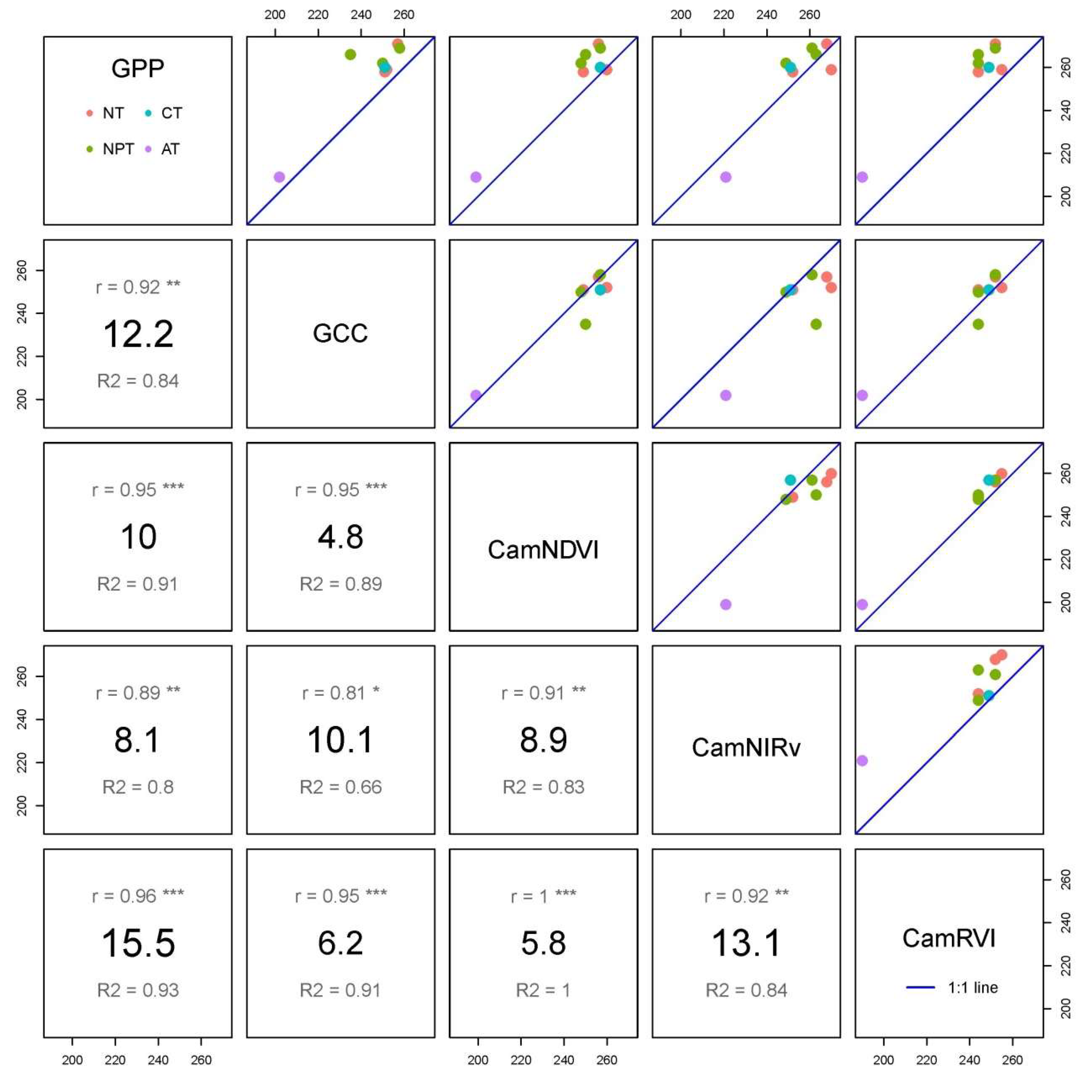
We show the PTDs derived from VIs differ from each other. For the widely used GCC and CamNDVI, the PTDs extracted from CamNDVI are delayed compared to the ones derived from the GCC, which is likely attributed to GCC, and is more sensitive to color changes, while CamNDVI is more sensitive to LAI and biomass.
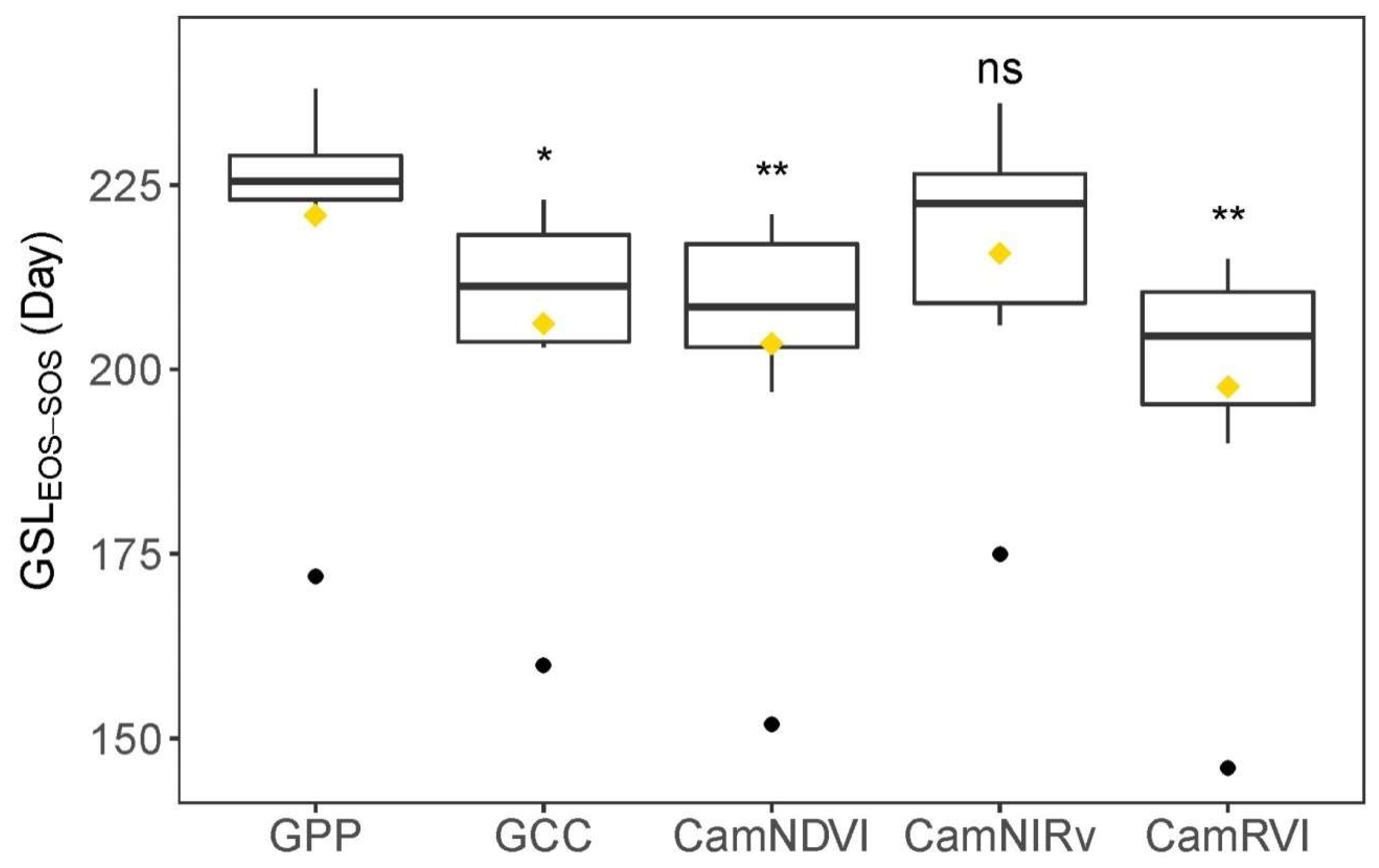
CamNIRv is best at representing the PTDs of GPP at the Green-up period, while CamNDVI is the best proxy to represent the PTDs of GPP at the Dry-down period. CamNIRv performs best regarding the representation of the GSL of GPP.
In summary, we show that it is possible to determine crucial PTDs of structural and physiological phenology through using near-infrared-enabled digital cameras. GPP could be well represented when combining the use of different VIs for this purpose.

Author Contributions

Conceptualization, M.M., M.R., C.R., and Y.L.; Methodology, Y.L., G.F., X.M., and M.M.; Formal Analysis, Y.L., and T.S.E.-M.; Supervision, M.M., M.R., C.R., and X.M., Investigation, B.A., R.G.-C., T.W.H., G.M., and M.P.M.; Data Curation, T.S.E.-M., R.G.-C., M.P.M., G.M., and T.W.H.; Writing-Original Draft Preparation, Y.L., Writing-Review & Editing, all coauthors.

Acknowledgments

The authors acknowledge the Alexander von Humboldt Foundation for supporting this research with the Max-Planck Prize to Markus Reichstein. Y.L. and M.M. gratefully acknowledge financial support from the China Scholarship Council. We are also thankful for financial support from the Spanish Ministry of Economy and Competitiveness through the FLUXPEC project “Monitoring changes in water and carbon fluxes from remote and proximal sensing in a Mediterranean dehesa ecosystem” (CGL2012-34383). The development of PhenoCam has been supported by the Northeastern States Research Cooperative, NSF’s Macrosystems Biology program (award EF-1065029 and EF-1702697), DOE’s Regional and Global Climate Modeling program (award DE-SC0016011), and the US National Park Service Inventory and Monitoring Program and the USA National Phenology Network (grant number G10AP00129 from the United States Geological Survey). The authors thank Sujan Koirala for relevant technical assistance and comments on graphics. The authors thank two anonymous reviewers and the editor for constructive comments to improve the earlier manuscript. The authors thank Andrew Durso for final proofreading for English.

Conflicts of Interest

The authors declare no conflict of interest.

Appendix A

Table A1. Mean air temperature (Ta_mean), sum of precipitation (Prec), and mean gross primary productivity (GPP) of different seasons at Majadas de Tiétar from hydrological year 2014 to 2016 (Hydro-2014 to Hydro-2016) 1.
AutumnWinterSpringSummer
(September–November)(December–February)(March–May)(June–July)
TaPrecGPPTaPrecGPPTaPrecGPPTaPrecGPP
(°C)(mm)(µmol m−2 s−1)(°C)(mm)(µmol m−2 s−1)(°C)(mm)(µmol m−2 s−1)(°C)(mm)(µmol m−2 s−1)
Hydro-201417.5333.44.76.4105.64.316.394.99.427.567.74.2
Hydro-201516.8296.03.69.4181.65.713.5281.711.726.414.17.0
Hydro-201617.2272.73.68.0205.95.216.494.08.927.346.44.2
1 Mean GPP is the average of day time (6:00–18:00) of GPP from Control tower (ES-LMa), Nitrogen tower (ES-LM1), Nitrogen and Phosphorous tower (ES-LM2) at Majadas de Tiétar.
Table A2. Comparison between phenological transition dates (PTDs) derived from PhenoCam-based green chromatic coordinate (GCC), normalized difference vegetation index (CamNDVI), near-infrared reflectance of vegetation index (CamNIRv), ratio vegetation index (CamRVI) and PTDs derived from GPP in four Mediterranean experimental sites 1.
Green-Up Period Dry-Down Period
GCCCamNDVICamNIRvCamRVIGCCCamNDVICamNIRvCamRVI
StatsUDSOStrsUDSOStrsUDSOStrsUDSOStrsEOStrsRDEOStrsRDEOStrsRDEOStrsRD
N888888881010101010101010
MAE (day)8.013.11417.54.82.81620.27.07.14.95.58.78.86.94.4
RMSE (day)10.610.414.5196.33.316.621.69.610.06.06.310.29.98.05.5
r0.610.640.940.770.910.980.910.750.900.910.940.940.910.950.920.95
p-value******nsns*******nsns**nsns
1 Statistics are computed using the PTDs at the Green-up period (including PTD UD, SOStrs, and POS1) and the Dry-down period (including PTD EOStrs, RD, and POS2). Here only show the statistics for UD, SOStrs, EOStrs, and RD which are most important in Green-up and Dry-down period. Please refer to each PTD in Table 2. N, number of observations; MAE, mean absolute error; RMSE, root mean squared error. p-values are as follows: *** p ≤ 0.001, ** 0.001 < p ≤ 0.01, * 0.01 < p ≤ 0.05, ns for p > 0.05.
Figure A1. Comparison between max (Sonnentag et al., 2012) and max.density methods for their performance of filtering the PhenoCam-based vegetation indexes like near-infrared reflectance of vegetation index (NIRv). The black points are original half-hourly NIRv data, while red points stand for the filtered daily NIRv data retrieved by using max or max.density method.
Remotesensing 10 01293 g0a1
Figure A2. Scatter plots between monthly mean air temperature (Ta), monthly sum of precipitation (Prec) and green chromatic coordinate (GCC) during day time of (a) autumn, (b) winter, (c) spring, and (d) summer in hydrological year 2014 to 2016 in four Mediterranean tree–grass ecosystem in Spain. The data in hydrological years of 2014, 2015 and 2016 are colored with green, red and blue color, respectively. The regression line and the formula are shown if the linear regression is statistically significant (p-value: p < 0.05). The gray area represents 95% confidence interval. R2: determination coefficient of linear regression.
Remotesensing 10 01293 g0a2
Figure A3. Scatter plots between monthly mean air temperature (Ta), monthly sum of precipitation (Prec) and gross primary productivity (GPP) during day time of (a) autumn, (b) winter, (c) spring, and (d) summer in hydrological year 2014 to 2016. The data in hydrological years of 2014, 2015 and 2016 are colored with green, red and blue color, respectively. The regression line and the formula are shown if the linear regression is statistically significant (p-value: p < 0.05). The gray area represents 95% confidence interval. R2: determination coefficient of linear regression.
Remotesensing 10 01293 g0a3
Figure A4. Matrix plots of growing season length (GSLRD-UD) calculated from different data source: gross primary productivity (GPP), PhenoCam-based green chromatic coordinate (GCC), normalized difference vegetation index (CamNDVI), near-infrared reflectance of vegetation index (CamNIRv), and ratio vegetation index (CamRVI). Upper right boxes display the scatterplots and 1:1 line. Lower left boxes show the mean absolute error (MAE (days); bold in the center), the Pearson’s correlation coefficient (r; gray colored in the top), and slope of linear regression (slope: gray colored in the bottom) between respective variables. p-values are for correlation test for respective variables and as follows: *** p ≤ 0.001, ** 0.001 < p ≤ 0.01, * 0.01 < p ≤ 0.05. Please see the definition of GSLRD-UD in the Table 2.
Remotesensing 10 01293 g0a4
Figure A5. Growing season length (GSLEOS-EOS) derived from gross primary productivity (GPP), PhenoCam-based green chromatic coordinate (GCC), normalized difference vegetation index (CamNDVI), near-infrared reflectance of vegetation index (CamNIRv), and ratio vegetation index (CamRVI) for four Mediterranean tree–grass ecosystems (FLUXNET IDs are ES-LM1, ES-LM2, ES-LMa, and ES-Abr, respectively). The gold squares stand for mean GSL in all site-years, while the black points stand for the GSL derived from ES-Abr. The statistically significant differences were tested between GPP and vegetation indexes—GCC, CamNDVI, CamNIRv and CamRVI. p-values are as follows: ** 0.001 < p ≤ 0.01, * 0.01 < p ≤ 0.05, ns for p > 0.05. Please see the definition of GSLEOS-SOS in the Table 2.
Remotesensing 10 01293 g0a5
Figure A6. Time series of green chromatic coordinate (GCC) computed for Grass, Tree and Ecosystem region of interest (ROI) in four experimental sites (FLUXNET IDs are ES-LM1, ES-LM2, ES-LMa, and ES-Abr, respectively) during year of 2014 to 2017. The increase of GCC for Tree ROI during spring is concomitant with the leaf flushing.
Remotesensing 10 01293 g0a6

Appendix B. The Procedures and Code for Extracting Phenological Transition Dates (PTDs)

The procedures to extract PTDs from time series of vegetation indexes (VIs) or gross primary productivity (GPP) are as follows (also referring to Figure A7:
  • Try to find interminD. The linking point of two peaks (interminD) is the minimum between the two peaks between the Julian day of the year (Doy) 150–250.
  • Once we found the interminD, the time series is split into two parts and for each part the main PTDs are computed. The date of POS is calculated by determining the date at which the maximum value of the time series (using f(t) to refer to the time series hereafter) is reached. Baseline and maxline are the minimum and maximum value in each part of f(t), respectively.
  • The maximum and minimum of the first derivative of the f(t) (f’(t)) represent the maximum slopes of the upward and downward period (dashed lines). The intersections between these lines and the baseline are defined as upward day (UD) and recession day (RD). UD stands for the value when the f(t) begins to increase during the Green-up period. RD stands for the value when the f(t) stops decreasing during the Dry-down period. The intersections between these lines and maxline are the saturating day (SD) and downward day (DD). The SD indicates when the plants begin to reach full greenness or maximum photosynthesis, while DD stands for the date when plants begin to senesce [61].
  • SOStrs and EOStrs are retrieved by computing the date when the value reaches 50% of the maximum in the upward and downward period, respectively [62].
The Code for extracting PTDs is shared in the attached file (PTD_extraction.R). You can also use the example in the attached example folder for a test to extract PTDs.
Figure A7. Procedures to extract phenological transition dates metrics (PTDs) from different vegetation indexes (VIs) or daily maximum gross primary productivity (GPP). The procedures for extracting PTDs from seasonal VIs or GPP trajectory f(t) are described in detail in the text of Appendix B (The number in the left of each panel corresponds to the order of procedures in the Appendix B). The black circles represent the original vegetation indexes value (CamGCC, CamNDVI, CamNIRv, CamRVI, or GPP). Results of the smoothing procedure are shown by red circles. The PTDs extracted in each step are highlighted with orange color, while the threshold values are indicated by the blue dotted line. The PTDs colored with dark green are the PTDs we study in this article. Their names are corresponding to UD, SOStrs, POS1, POS2, EOStrs, and RD in the Table 2, respectively.
Remotesensing 10 01293 g0a7

References

  1. Dubé, P.; Perry, L.P.; Vittum, M. Instructions for Phenological Observations: Lilac and Honeysuckle; Bulletin/Vermont Agricultural Experiment Station: Burlington, NJ, USA, 1984. [Google Scholar]
  2. Lieth, H. Purposes of a phenology book. In Phenology and Seasonality Modeling; Springer: Berlin, Germany, 1974; pp. 3–19. [Google Scholar]
  3. Hollinger, D.Y.; Ollinger, S.; Richardson, A.; Meyers, T.; Dail, D.; Martin, M.; Scott, N.; Arkebauer, T.; Baldocchi, D.; Clark, K.; et al. Albedo estimates for land surface models and support for a new paradigm based on foliage nitrogen concentration. Glob. Chang. Boil. 2010, 16, 696–710. [Google Scholar] [CrossRef] [Green Version]
  4. Keenan, T.F.; Gray, J.; Friedl, M.A.; Toomey, M.; Bohrer, G.; Hollinger, D.Y.; Munger, J.W.; O’Keefe, J.; Schmid, H.P.; Wing, I.S.; et al. Net carbon uptake has increased through warming-induced changes in temperate forest phenology. Nat. Clim. Chang. 2014, 4, 598–604. [Google Scholar] [CrossRef]
  5. Peñuelas, J.; Rutishauser, T.; Filella, I. Phenology feedbacks on climate change. Science 2009, 324, 887. [Google Scholar] [CrossRef] [PubMed] [Green Version]
  6. Richardson, A.D.; Keenan, T.F.; Migliavacca, M.; Ryu, Y.; Sonnentag, O.; Toomey, M. Climate change, phenology, and phenological control of vegetation feedbacks to the climate system. Agric. For. Meteorol. 2013, 169, 156–173. [Google Scholar] [CrossRef]
  7. Forkel, M.; Migliavacca, M.; Thonicke, K.; Reichstein, M.; Schaphoff, S.; Weber, U.; Carvalhais, N. Co-dominant water control on global inter-annual variability and trends in land surface phenology and greenness. Glob. Chang. Boil. 2015, 21, 3414–3435. [Google Scholar] [CrossRef] [PubMed]
  8. Randerson, J.T.; Hoffman, F.M.; Thornton, P.E.; Mahowald, N.M.; Lindsay, K.; Lee, Y.H.; Nevison, C.D.; Doney, S.C.; Bonan, G.; Stöckli, R.; et al. Systematic assessment of terrestrial biogeochemistry in coupled climate–carbon models. Glob. Chang. Boil. 2009, 15, 2462–2484. [Google Scholar] [CrossRef]
  9. Richardson, A.D.; Anderson, R.S.; Arain, M.A.; Barr, A.G.; Bohrer, G.; Chen, G.; Chen, J.M.; Ciais, P.; Davis, K.J.; Desai, A.R.; et al. Terrestrial biosphere models need better representation of vegetation phenology: Results from the North American Carbon Program Site Synthesis. Glob. Chang. Boil. 2012, 18, 566–584. [Google Scholar] [CrossRef] [Green Version]
  10. Migliavacca, M.; Sonnentag, O.; Keenan, T.F.; Cescatti, A.; O’Keefe, J.; Richardson, A.D. On the uncertainty of phenological responses to climate change, and implications for a terrestrial biosphere model. Biogeosciences 2012, 9, 2063–2083. [Google Scholar] [CrossRef] [Green Version]
  11. Tang, J.; Körner, C.; Muraoka, H.; Piao, S.; Shen, M.; Thackeray, S.J.; Yang, X. Emerging opportunities and challenges in phenology: A review. Ecosphere 2016, 7, e01436. [Google Scholar] [CrossRef]
  12. Menzel, A. Phenology: Its importance to the global change community. Clim. Chang. 2002, 54, 379–385. [Google Scholar] [CrossRef]
  13. Basler, D.; Körner, C. Photoperiod sensitivity of bud burst in 14 temperate forest tree species. Agric. For. Meteorol. 2012, 165, 73–81. [Google Scholar] [CrossRef]
  14. Fu, Y.H.; Zhao, H.; Piao, S.; Peaucelle, M.; Peng, S.; Zhou, G.; Ciais, P.; Huang, M.; Menzel, A.; Peñuelas, J.; et al. Declining global warming effects on the phenology of spring leaf unfolding. Nature 2015, 526, 104–107. [Google Scholar] [CrossRef] [PubMed] [Green Version]
  15. Menzel, A. A 500 year pheno-climatological view on the 2003 heatwave in Europe assessed by grape harvest dates. Meteorol. Z. 2005, 14, 75–77. [Google Scholar] [CrossRef]
  16. Menzel, A.; Sparks, T.H.; Estrella, N.; Koch, E.; Aasa, A.; Ahas, R.; Alm-KÜBler, K.; Bissolli, P.; BraslavskÁ, O.G.; Briede, A.; et al. European phenological response to climate change matches the warming pattern. Glob. Chang. Boil. 2006, 12, 1969–1976. [Google Scholar] [CrossRef] [Green Version]
  17. Richardson, A.D.; Klosterman, S.; Toomey, M. Near-surface sensor-derived phenology. In Phenology: An Integrative Environmental Science; Springer: Berlin, Germany, 2013; pp. 413–430. [Google Scholar]
  18. Hufkens, K.; Friedl, M.; Sonnentag, O.; Braswell, B.H.; Milliman, T.; Richardson, A.D. Linking near-surface and satellite remote sensing measurements of deciduous broadleaf forest phenology. Remote Sens. Environ. 2012, 117, 307–321. [Google Scholar] [CrossRef]
  19. Ide, R.; Oguma, H. Use of digital cameras for phenological observations. Ecol. Inform. 2010, 5, 339–347. [Google Scholar] [CrossRef]
  20. Migliavacca, M.; Galvagno, M.; Cremonese, E.; Rossini, M.; Meroni, M.; Sonnentag, O.; Cogliati, S.; Manca, G.; Diotri, F.; Busetto, L.; et al. Using digital repeat photography and eddy covariance data to model grassland phenology and photosynthetic CO2 uptake. Agric. For. Meteorol. 2011, 151, 1325–1337. [Google Scholar] [CrossRef]
  21. Motohka, T.; Nasahara, K.N.; Oguma, H.; Tsuchida, S. Applicability of green-red vegetation index for remote sensing of vegetation phenology. Remote Sens. 2010, 2, 2369–2387. [Google Scholar] [CrossRef]
  22. Sonnentag, O.; Hufkens, K.; Teshera-Sterne, C.; Young, A.M.; Friedl, M.; Braswell, B.H.; Milliman, T.; O’Keefe, J.; Richardson, A.D. Digital repeat photography for phenological research in forest ecosystems. Agric. For. Meteorol. 2012, 152, 159–177. [Google Scholar] [CrossRef]
  23. Zhao, J.; Zhang, Y.; Tan, Z.; Song, Q.; Liang, N.; Yu, L.; Zhao, J. Using digital cameras for comparative phenological monitoring in an evergreen broad-leaved forest and a seasonal rain forest. Ecol. Inform. 2012, 10, 65–72. [Google Scholar] [CrossRef]
  24. Brown, T.B.; Hultine, K.R.; Steltzer, H.; Denny, E.G.; Denslow, M.W.; Granados, J.; Henderson, S.; Moore, D.; Nagai, S.; SanClements, M.; et al. Using phenocams to monitor our changing Earth: Toward a global phenocam network. Front. Ecol. Environ. 2016, 14, 84–93. [Google Scholar] [CrossRef]
  25. Keller, M.; Schimel, D.S.; Hargrove, W.W.; Hoffman, F.M. A continental strategy for the National Ecological Observatory Network. Front. Ecol. Environ. 2008, 6, 282–284. [Google Scholar] [CrossRef] [Green Version]
  26. Nasahara, K.N.; Nagai, S. Review: Development of an in situ observation network for terrestrial ecological remote sensing: The Phenological Eyes Network (PEN). Ecol. Res. 2015, 30, 211–223. [Google Scholar] [CrossRef]
  27. Richardson, A.D.; Braswell, B.H.; Hollinger, D.Y.; Jenkins, J.P.; Ollinger, S.V. Near-surface remote sensing of spatial and temporal variation in canopy phenology. Ecol. Appl. 2009, 19, 1417–1428. [Google Scholar] [CrossRef] [PubMed]
  28. Wingate, L.; Ogée, J.; Cremonese, E.; Filippa, G.; Mizunuma, T.; Migliavacca, M.; Moisy, C.; Wilkinson, M.; Moureaux, C.; Wohlfahrt, G.; et al. Interpreting canopy development and physiology using a European phenology camera network at flux sites. Biogeosciences 2015, 12, 5995–6015. [Google Scholar] [CrossRef] [Green Version]
  29. Petach, A.R.; Toomey, M.; Aubrecht, D.M.; Richardson, A.D. Monitoring vegetation phenology using an infrared-enabled security camera. Agric. For. Meteorol. 2014, 195, 143–151. [Google Scholar] [CrossRef] [Green Version]
  30. Moore, C.E.; Beringer, J.; Evans, B.; Hutley, L.B.; Tapper, N.J. Tree–grass phenology information improves light use efficiency modelling of gross primary productivity for an Australian tropical savanna. Biogeosciences 2017, 14, 111–129. [Google Scholar] [CrossRef]
  31. Richardson, A.D.; Black, T.A.; Ciais, P.; Delbart, N.; Friedl, M.A.; Gobron, N.; Hollinger, D.Y.; Kutsch, W.L.; Longdoz, B.; Luyssaert, S.; et al. Influence of spring and autumn phenological transitions on forest ecosystem productivity. Philos. Trans. R. Soc. B Boil. Sci. 2010, 365, 3227–3246. [Google Scholar] [CrossRef] [PubMed] [Green Version]
  32. Toomey, M.; Friedl, M.A.; Frolking, S.; Hufkens, K.; Klosterman, S.; Sonnentag, O.; Baldocchi, D.D.; Bernacchi, C.J.; Biraud, S.C.; Bohrer, G.; et al. Greenness indices from digital cameras predict the timing and seasonal dynamics of canopy-scale photosynthesis. Ecol. Appl. 2015, 25, 99–115. [Google Scholar] [CrossRef] [PubMed] [Green Version]
  33. Richardson, A.D.; Hollinger, D.Y.; Dail, D.B.; Lee, J.T.; Munger, J.W.; O’Keefe, J. Influence of spring phenology on seasonal and annual carbon balance in two contrasting New England forests. Tree Physiol. 2009, 29, 321–331. [Google Scholar] [CrossRef] [PubMed] [Green Version]
  34. Filippa, G.; Cremonese, E.; Migliavacca, M.; Galvagno, M.; Sonnentag, O.; Humphreys, E.; Hufkens, K.; Ryu, Y.; Verfaillie, J.; di Cella, U.M.; et al. NDVI derived from near-infrared-enabled digital cameras: Applicability across different plant functional types. Agric. For. Meteorol. 2018, 249, 275–285. [Google Scholar] [CrossRef]
  35. Yang, H.; Yang, X.; Heskel, M.; Sun, S.; Tang, J. Seasonal variations of leaf and canopy properties tracked by ground-based NDVI imagery in a temperate forest. Sci. Rep. 2017, 7, 1267. [Google Scholar] [CrossRef] [PubMed]
  36. Filippa, G.; Cremonese, E.; Migliavacca, M.; Galvagno, M.; Forkel, M.; Wingate, L.; Tomelleri, E.; di Cella, U.M.; Richardson, A.D. Phenopix: AR package for image-based vegetation phenology. Agric. For. Meteorol. 2016, 220, 141–150. [Google Scholar] [CrossRef]
  37. Elmore, A.J.; Guinn, S.M.; Minsley, B.J.; Richardson, A.D. Landscape controls on the timing of spring, autumn, and growing season length in mid-Atlantic forests. Glob. Chang. Boil. 2012, 18, 656–674. [Google Scholar] [CrossRef]
  38. Graham, E.A.; Riordan, E.C.; Yuen, E.M.; Estrin, D.; Rundel, P.W. Public Internet-connected cameras used as a cross-continental ground-based plant phenology monitoring system. Glob. Chang. Boil. 2010, 16, 3014–3023. [Google Scholar] [CrossRef]
  39. Klosterman, S.; Hufkens, K.; Gray, J.; Melaas, E.; Sonnentag, O.; Lavine, I.; Mitchell, L.; Norman, R.; Friedl, M.; Richardson, A. Evaluating remote sensing of deciduous forest phenology at multiple spatial scales using PhenoCam imagery. Biogeosciences 2014, 11, 4305–4320. [Google Scholar] [CrossRef] [Green Version]
  40. Liang, L.; Schwartz, M.D.; Fei, S. Validating satellite phenology through intensive ground observation and landscape scaling in a mixed seasonal forest. Remote Sens. Environ. 2011, 115, 143–157. [Google Scholar] [CrossRef]
  41. Badgley, G.; Field, C.B.; Berry, J.A. Canopy near-infrared reflectance and terrestrial photosynthesis. Sci. Adv. 2017, 3, e1602244. [Google Scholar] [CrossRef] [PubMed] [Green Version]
  42. Chen, J.M. Evaluation of vegetation indices and a modified simple ratio for boreal applications. Can. J. Remote Sens. 1996, 22, 229–242. [Google Scholar] [CrossRef]
  43. Liu, Y.; Hill, M.J.; Zhang, X.; Wang, Z.; Richardson, A.D.; Hufkens, K.; Filippa, G.; Baldocchi, D.D.; Ma, S.; Verfaillie, J.; et al. Using data from Landsat, MODIS, VIIRS and PhenoCams to monitor the phenology of California oak/grass savanna and open grassland across spatial scales. Agric. For. Meteorol. 2017, 237–238, 311–325. [Google Scholar] [CrossRef]
  44. Moore, C.E.; Beringer, J.; Evans, B.; Hutley, L.B.; Tapper, N.J. Tree-grass phenology information improves light use efficiency modelling of gross primary productivity for an Australian tropical savanna. Biogeosciences 2017, 14, 111–129. [Google Scholar] [CrossRef]
  45. Beringer, J.; Hutley, L.B.; Abramson, D.; Arndt, S.K.; Briggs, P.; Bristow, M.; Canadell, J.G.; Cernusak, L.A.; Eamus, D.; Edwards, A.C.; et al. Fire in Australian savannas: From leaf to landscape. Glob. Chang. Boil. 2015, 21, 62–81. [Google Scholar] [CrossRef] [PubMed] [Green Version]
  46. Grace, J.; Jose, J.S.; Meir, P.; Miranda, H.S.; Montes, R.A. Productivity and carbon fluxes of tropical savannas. J. Biogeogr. 2006, 33, 387–400. [Google Scholar] [CrossRef]
  47. Hanan, N.; Hill, M. Savannas in a Changing Earth System: The NASA Terrestrial Ecology Tree-Grass Project. White Paper for the NASA Terrestrial Ecology Program; Earth Science Division: Washington, DC, USA, 2012. [Google Scholar]
  48. Migliavacca, M.; Reichstein, M.; Richardson, A.D.; Mahecha, M.D.; Cremonese, E.; Delpierre, N.; Galvagno, M.; Law, B.E.; Wohlfahrt, G.; Andrew Black, T.; et al. Influence of physiological phenology on the seasonal pattern of ecosystem respiration in deciduous forests. Glob. Chang. Boil. 2015, 21, 363–376. [Google Scholar] [CrossRef] [PubMed]
  49. Perez-Priego, O.; El-Madany, T.S.; Migliavaca, M.; Kowalski, A.S.; Jung, M.; Carrara, A.; Kolle, O.; Martín, M.P.; Pacheco-Labrador, J.; Moreno, G.; et al. Evaluation of eddy covariance latent heat fluxes with independent lysimeter and sapflow estimates in a Mediterranean savannah ecosystem. Agric. For. Meteorol. 2017, 236, 87–99. [Google Scholar] [CrossRef]
  50. Wilczak, J.M.; Oncley, S.P.; Stage, S.A. Sonic anemometer tilt correction algorithms. Bound.-Lay. Meteorol. 2001, 99, 127–150. [Google Scholar] [CrossRef]
  51. Moncrieff, J.; Clement, R.; Finnigan, J.; Meyers, T. Averaging, detrending, and filtering of eddy covariance time series. In Handbook of Micrometeorology; Springer: Berlin, Germany, 2004; pp. 7–31. [Google Scholar]
  52. Moncrieff, J.B.; Massheder, J.; De Bruin, H.; Elbers, J.; Friborg, T.; Heusinkveld, B.; Kabat, P.; Scott, S.; Soegaard, H.; Verhoef, A. A system to measure surface fluxes of momentum, sensible heat, water vapour and carbon dioxide. J. Hydrol. 1997, 188, 589–611. [Google Scholar] [CrossRef]
  53. Mauder, M.; Foken, T. Documentation and Instruction Manual of the Eddy-Covariance Software Package TK3; University of Bayreuth: Bayreuth, Germany, 2011. [Google Scholar]
  54. Rebmann, C.; Göckede, M.; Foken, T.; Aubinet, M.; Aurela, M.; Berbigier, P.; Bernhofer, C.; Buchmann, N.; Carrara, A.; Cescatti, A.; et al. Quality analysis applied on eddy covariance measurements at complex forest sites using footprint modelling. Theor. Appl. Clim. 2005, 80, 121–141. [Google Scholar] [CrossRef]
  55. Papale, D.; Reichstein, M.; Aubinet, M.; Canfora, E.; Bernhofer, C.; Kutsch, W.; Longdoz, B.; Rambal, S.; Valentini, R.; Vesala, T.; et al. Towards a standardized processing of Net Ecosystem Exchange measured with eddy covariance technique: Algorithms and uncertainty estimation. Biogeosciences 2006, 3, 571–583. [Google Scholar] [CrossRef]
  56. Reichstein, M.; Falge, E.; Baldocchi, D.; Papale, D.; Aubinet, M.; Berbigier, P.; Bernhofer, C.; Buchmann, N.; Gilmanov, T.; Granier, A. On the separation of net ecosystem exchange into assimilation and ecosystem respiration: Review and improved algorithm. Glob. Chang. Boil. 2005, 11, 1424–1439. [Google Scholar] [CrossRef]
  57. Wutzler, T.; Lucas-Moffat, A.; Migliavacca, M.; Knauer, J.; Sickel, K.; Šigut, L.; Menzer, O.; Reichstein, M. Basic and extensible post-processing of eddy covariance flux data with REddyProc. Biogeosci. Discuss. 2018. [Google Scholar] [CrossRef]
  58. Pacheco-Labrador, J.; El-Madany, T.S.; Martín, M.P.; Migliavacca, M.; Rossini, M.; Carrara, A.; Zarco-Tejada, P.J. Spatio-Temporal Relationships between Optical Information and Carbon Fluxes in a Mediterranean Tree-Grass Ecosystem. Remote Sens. 2017, 9, 608. [Google Scholar] [CrossRef]
  59. EI-Madany, T.S.; Reichstein, M.; Perez-Priego, O.; Carrara, A.; Moreno, G.; Martín, M.P.; Pacheco-Labrador, J.; Wohlfahrt, G.; Nieto, H.; Weber, U.; et al. Drivers of spatio-temporal variability of carbon dioxide and energy fluxes in a Mediterranean savanna ecosystem. Agric. For. Meteorol. 2018, 262, 258–278. [Google Scholar] [CrossRef]
  60. Von Buttlar, J.; Zscheischler, J.; Mahecha, M.D. An extended approach for spatiotemporal gapfilling: Dealing with large and systematic gaps in geoscientific datasets. Nonlinear Process. Geophys. 2014, 21, 203–215. [Google Scholar] [CrossRef]
  61. Gu, L.; Post, W.M.; Baldocchi, D.D.; Black, T.A.; Suyker, A.E.; Verma, S.B.; Vesala, T.; Wofsy, S.C. Characterizing the seasonal dynamics of plant community photosynthesis across a range of vegetation types. In Phenology of Ecosystem Processes; Springer: Berlin, Germany, 2009; pp. 35–58. [Google Scholar]
  62. White, M.A.; Thornton, P.E.; Running, S.W. A continental phenology model for monitoring vegetation responses to interannual climatic variability. Glob. Biogeochem. Cycles 1997, 11, 217–234. [Google Scholar] [CrossRef] [Green Version]
  63. Team, R.C. R: A Language and Environment for Statistical Computing 2014 [Internet]; R Foundation for Statistical Computing: Vienna, Austria, 2015. [Google Scholar]
  64. Baldocchi, D.D.; Xu, L.; Kiang, N. How plant functional-type, weather, seasonal drought, and soil physical properties alter water and energy fluxes of an oak–grass savanna and an annual grassland. Agric. For. Meteorol. 2004, 123, 13–39. [Google Scholar] [CrossRef] [Green Version]
  65. Moreno, G.; Cubera, E. Impact of stand density on water status and leaf gas exchange in Quercus ilex. For. Ecol. Manag. 2008, 254, 74–84. [Google Scholar] [CrossRef]
  66. Rolo, V.; Moreno, G. Interspecific competition induces asymmetrical rooting profile adjustments in shrub-encroached open oak woodlands. Trees 2012, 26, 997–1006. [Google Scholar] [CrossRef]
  67. Ward, D.; Wiegand, K.; Getzin, S. Walter’s two-layer hypothesis revisited: Back to the roots! Oecologia 2013, 172, 617–630. [Google Scholar] [CrossRef] [PubMed]
  68. Hatfield, J.L.; Prueger, J.H. Temperature extremes: Effect on plant growth and development. Weather Clim. Extremes 2015, 10, 4–10. [Google Scholar] [CrossRef]
  69. Allard, V.; Ourcival, J.; Rambal, S.; Joffre, R.; Rocheteau, A. Seasonal and annual variation of carbon exchange in an evergreen Mediterranean forest in southern France. Glob. Chang. Boil. 2008, 14, 714–725. [Google Scholar] [CrossRef]
  70. Diodato, N.; Bellocchi, G. Modelling vegetation greenness responses to climate variability in a Mediterranean terrestrial ecosystem. Environ. Monit. Assess. 2008, 143, 147–159. [Google Scholar] [CrossRef] [PubMed]
  71. Ma, S.; Baldocchi, D.D.; Xu, L.; Hehn, T. Inter-annual variability in carbon dioxide exchange of an oak/grass savanna and open grassland in California. Agric. For. Meteorol. 2007, 147, 157–171. [Google Scholar] [CrossRef]
  72. Sippel, S.; El-Madany, T.S.; Migliavacca, M.; Mahecha, M.D.; Carrara, A.; Flach, M.K.T.; Thonicke, K.; Vossbeck, M.; Reichstein, M. Warm Winter, Wet Spring and an Extreme Response in Ecosystem Functioning on the Iberian Peninsula. Special issue: Explaining Extreme Events from a Climate Perspective. Bull. Am. Meteor. Soc. 2018, 98, 80–85. [Google Scholar] [CrossRef]
  73. Choler, P.; Sea, W.; Briggs, P.; Raupach, M.; Leuning, R. A simple ecohydrological model captures essentials of seasonal leaf dynamics in semi-arid tropical grasslands. Biogeosciences 2010, 7, 907–920. [Google Scholar] [CrossRef] [Green Version]
  74. Hufkens, K.; Keenan, T.F.; Flanagan, L.B.; Scott, R.L.; Bernacchi, C.J.; Joo, E.; Brunsell, N.A.; Verfaillie, J.; Richardson, A.D. Productivity of North American grasslands is increased under future climate scenarios despite rising aridity. Nat. Clim. Chang. 2016, 6, 710–714. [Google Scholar] [CrossRef]
  75. Keenan, T.; Darby, B.; Felts, E.; Sonnentag, O.; Friedl, M.; Hufkens, K.; O’Keefe, J.; Klosterman, S.; Munger, J.W.; Toomey, M.; et al. Tracking forest phenology and seasonal physiology using digital repeat photography: A critical assessment. Ecol. Appl. 2014, 24, 1478–1489. [Google Scholar] [CrossRef] [PubMed] [Green Version]
  76. Ryu, Y.; Lee, G.; Jeon, S.; Song, Y.; Kimm, H. Monitoring multi-layer canopy spring phenology of temperate deciduous and evergreen forests using low-cost spectral sensors. Remote Sens. Environ. 2014, 149, 227–238. [Google Scholar] [CrossRef]
  77. Yang, X.; Tang, J.; Mustard, J.F. Beyond leaf color: Comparing camera-based phenological metrics with leaf biochemical, biophysical, and spectral properties throughout the growing season of a temperate deciduous forest. J. Geophys. Res. Biogeosci. 2014, 119, 181–191. [Google Scholar] [CrossRef] [Green Version]
  78. Migliavacca, M.; Perez-Priego, O.; Rossini, M.; El-Madany, T.S.; Moreno, G.; van der Tol, C.; Rascher, U.; Berninger, A.; Bessenbacher, V.; Burkart, A.; et al. Plant functional traits and canopy structure control the relationship between photosynthetic CO2 uptake and far-red sun-induced fluorescence in a Mediterranean grassland under different nutrient availability. New Phytol. 2017, 214, 1078–1091. [Google Scholar] [CrossRef] [PubMed]
  79. Viña, A.; Gitelson, A.A.; Nguy-Robertson, A.L.; Peng, Y. Comparison of different vegetation indices for the remote assessment of green leaf area index of crops. Remote Sens. Environ. 2011, 115, 3468–3478. [Google Scholar] [CrossRef]
  80. Vrieling, A.; Meroni, M.; Darvishzadeh, R.; Skidmore, A.K.; Wang, T.; Zurita-Milla, R.; Oosterbeek, K.; O’Connor, B.; Paganini, M. Vegetation phenology from Sentinel-2 and field cameras for a Dutch barrier island. Remote Sens. Environ. 2018, 215, 517–529. [Google Scholar] [CrossRef]
  81. Linderholm, H.W. Growing season changes in the last century. Agric. For. Meteorol. 2006, 137, 1–14. [Google Scholar] [CrossRef]
  82. Churkina, G.; Schimel, D.; Braswell, B.H.; Xiao, X. Spatial analysis of growing season length control over net ecosystem exchange. Glob. Chang. Boil. 2005, 11, 1777–1787. [Google Scholar] [CrossRef]
  83. White, M.; Running, S.; Thornton, P. The impact of growing-season length variability on carbon assimilation and evapotranspiration over 88 years in the eastern US deciduous forest. Int. J. Biometeorol. 1999, 42, 139–145. [Google Scholar] [CrossRef] [PubMed]
  84. Yengoh, G.T.; Dent, D.; Olsson, L.; Tengberg, A.E.; Tucker, C.J., III. Use of the Normalized Difference Vegetation Index (NDVI) to Assess Land Degradation at Multiple Scales: Current Status, Future Trends, and Practical Considerations; Springer: Berlin, Germany, 2015. [Google Scholar]
  85. Peng, Y.; Gitelson, A.A. Application of chlorophyll-related vegetation indices for remote estimation of maize productivity. Agric. For. Meteorol. 2011, 151, 1267–1276. [Google Scholar] [CrossRef]
  86. Jiang, Z.; Huete, A.R.; Didan, K.; Miura, T. Development of a two-band enhanced vegetation index without a blue band. Remote Sens. Environ. 2008, 112, 3833–3845. [Google Scholar] [CrossRef]
  87. Yang, J.; Tian, H.; Pan, S.; Chen, G.; Zhang, B.; Dangal, S. Amazon droughts and forest responses: Largely reduced forest photosynthesis but slightly increased canopy greenness during the extreme drought of 2015/2016. Glob. Chang. Boil. 2018. [Google Scholar] [CrossRef] [PubMed]
Figure 1. (left panel) Experimental setup at Majadas de Tiétar and La Albuera in Spain and (right panel) an example of regions of interest (ROIs) in each experimental site: Grass, Tree and Ecosystem ROIs, respectively. At each site, an eddy covariance (EC) system was installed at a height of 15 m to measure the fluxes of the whole ecosystem. A near-infrared-enabled camera was installed at 15 m beside the EC system to take pictures half-hourly between 10:00 and 14:30. Three EC towers are in the Majadas de Tiétar (FLUXNET IDs are ES-LM1, ES-LM2, and ES-LMa, respectively) and an EC tower is in the La Albuera (FLUX ID: ES-Abr), respectively (not shown). The map of Majadas de Tiétar was provided courtesy of the Spanish Program of Aerial Orthophotography. The design of the schematic plot of instruments in the experimental sites refers to [17] and the photo of the EC tower inside the graphic was taken by T.S. El-Madany.
Remotesensing 10 01293 g001
Figure 2. Conceptual figure of the seasonal dynamic of green chromatic coordinates (GCC), PhenoCam-based normalized difference vegetation index (CamNDVI), near-infrared reflectance of vegetation index (CamNIRv), ratio vegetation indexes (CamRVI), or daily maximum gross primary productivity (GPP), as well as their phenological transition dates (PTDs) for a “hydrological year”. The black circles represent the original vegetation indexes value (CamGCC, CamNDVI, CamNIRv, CamRVI, or GPP). Results of the smoothing procedure and its uncertainty are shown by red circles and gray area, respectively. The vertical dashed lines represent the PTDs and the corresponding names are shown: UD, SOStrs, POS1, POS2, EOStrs, RD. Two periods are most focused upon in this study: the Green-up period during autumn to winter (green rectangle which including UD, SOStrs, and POS1) and Dry-down period in late spring to summer (light-red rectangle that including POS2, EOStrs and RD). The time interval between UD and RD is defined as the growing season which indicated in the figure. Detailed description of PTDs and the other phenological terms are reported in the Table 2.
Remotesensing 10 01293 g002
Figure 3. Time series of PhenoCam-based green chromatic coordinate (GCC), normalized difference vegetation index (CamNDVI), near-infrared reflectance of vegetation index (CamNIRv), ratio vegetation index (CamRVI), maximum gross primary productivity (GPP), and meteorological variables (temperature and precipitation) for four Mediterranean tree–grass ecosystems (FLUXNET IDs are ES-LM1, ES-LM2, ES-LMa, and ES-Abr, respectively). Daily mean temperature (Ta) and total precipitation (Prec) of the Majadas de Tiétar (Maj) and La Albuera (Ala) are shown in the bottom panel.
Remotesensing 10 01293 g003
Figure 4. Scatter plots between monthly mean air temperature (Ta), monthly sum of precipitation (Prec), and monthly mean gross primary productivity (GPP) during day time of (a,b) winter, and (c,d) spring in hydrological year 2014 to 2016 in four Mediterranean tree–grass ecosystem in Spain. The data in hydrological years of 2014, 2015, and 2016 are colored with green, red, and blue color, respectively. The regression line and the formula are shown if the linear regression is statistically significant (p < 0.05). The gray area represents 95% confidence interval. R2: determination coefficient of linear regression.
Remotesensing 10 01293 g004
Figure 5. Barplots of the differences between phenological transition dates (PTDs) extracted from different PhenoCam-based vegetation indexes: green chromatic coordinate (GCC), normalized difference vegetation index (CamNDVI), near-infrared reflectance of vegetation index (CamNIRv), ratio vegetation index (CamRVI). The error bars represent the standard error of the PTDs derived from different experimental sites, and hydrological years. The statistically significant differences were tested using Wilcoxon signed-rank tests (when PTDs were not normally distributed) and paired Student’s t tests (when PTDs were normally distributed). p-values are as follows: *** p ≤ 0.001, ** 0.001 < p ≤ 0.01, * 0.01 < p ≤ 0.05, ns for p > 0.05. Please see the definition of each PTD in the Table 2.
Remotesensing 10 01293 g005
Figure 6. Comparison of phenological transition dates (PTDs) extracted from vegetation indexes (VIs): PhenoCam-based green chromatic coordinate (GCC), normalized difference vegetation index (CamNDVI), near-infrared reflectance of vegetation index (CamNIRv), ratio vegetation index (CamRVI), and gross primary productivity (GPP). Please see the definition of each PTD in the Table 2.
Remotesensing 10 01293 g006
Figure 7. Barplots of the differences between phenological transition dates (PTDs) extracted from different PhenoCam-based vegetation indexes (green chromatic coordinate (GCC), normalized difference vegetation index (CamNDVI), near-infrared reflectance of vegetation index (CamNIRv), ratio vegetation index (CamRVI)) and gross primary productivity (GPP). The error bars represent the standard error of the PTDs derived from different experimental sites, and hydrological years. The statistically significant differences were tested using Wilcoxon signed-rank tests (when PTDs were not normally distributed) and paired Student’s t tests (when PTDs were normally distributed). p-values are as follows: *** p ≤ 0.001, ** 0.001 < p ≤ 0.01, * 0.01 < p ≤ 0.05, ns for p > 0.05. Please see the definition of each PTD in the Table 2.
Remotesensing 10 01293 g007
Figure 8. Growing season length (GSLRD-UD) derived from gross primary productivity (GPP), PhenoCam-based green chromatic coordinate (GCC), normalized difference vegetation index (CamNDVI), near-infrared reflectance of vegetation index (CamNIRv), and ratio vegetation index (CamRVI) for four Mediterranean tree–grass ecosystems (FLUXNET IDs are ES-LM1, ES-LM2, ES-LMa, and ES-Abr, respectively). The gold squares stand for mean GSL in all site-years, while the black points stand for the GSL derived from ES-Abr. Data from ES-LM1, ES-LM2, and ES-LMa falling outside the 10%–90% percentile range are plotted as cross. The statistically significant differences were tested between GPP and vegetation indexes—GCC, CamNDVI, CamNIRv, and CamRVI. p-values are as follows: * 0.01 < p ≤ 0.05, ns for p > 0.05. Please see the definition of GSLRD-UD in the Table 2.
Remotesensing 10 01293 g008
Table 1. Results of the linear regression between normalized difference vegetation index (NDVI), near-infrared reflectance of vegetation index (NIRv), ratio vegetation index (RVI) retrieved from PhenoCam and spectral reflectance sensor (SRS) at four experimental sites 1.
SiteVIsNInterceptSlopeR2
ES-LM1NDVI40000.601.510.69
NIRv32820.060.010.60
RVI3389−2.036.610.54
ES-LM2NDVI43400.561.120.77
NIRv42230.040.010.55
RVI4268−0.143.550.57
ES-LMaNDVI35490.670.890.89
NIRv35220.060.010.73
RVI3515−0.205.170.84
ES-AbrNDVI35600.641.180.83
NIRv33610.060.010.82
RVI3564−0.785.390.80
1 ES-LM1, ES-LM2, ES-LMa, and ES-Abr are the FLUXNET-IDs of four experimental sites, respectively. N, number of observations used for each regression; Intercept and slope: the parameters of the linear regression between indexes retrieved from the PhenoCam and SRS; R2: determination coefficient of linear regression. Regression coefficients are all statistically significant (p < 0.001).
Table 2. Terms used in this study to describe the phenological transition dates (PTDs) and phenological periods.
TermsDescription
Phenological Transition Dates (PTDs)UDUpturn day in the green up period in the autumn
SOStrsWhen 50% of amplitude in the green up period in the autumn is reached
POS1When the first peak of season is reached
POS2When the second peak of season is reached
EOStrsWhen 50% of amplitude in the senescent period in the summer is reached
RDRecession day at the end of senescent period in the summer
Phenological periodsGreen-upGreenness/GPP increasing period in the autumn (including UD, SOStrs, and POS1)
Dry-downGreenness/GPP decreasing period in the summer (including POS2, EOStrs and RD)
GSLRD-UDGrowing season length defined in the hydrological year (day length between UD and RD)
GSLEOS-SOSGrowing season length defined for comparison with GSLRD-UD (day length between EOStrs and SOStrs, which is widely used in land surface phenology)
Table 3. Statistics between daily time series of vegetation indexes (PhenoCam-based green chromatic coordinates (GCC), normalized difference vegetation index (CamNDVI), near-infrared reflectance of vegetation index (CamNIRv), ratio vegetation index (CamRVI)) and gross primary productivity (GPP) at four experimental sites 1.
SiteVIs-GPPNr
ES-LM1GCC10960.90
CamNDVI10960.91
CamNIRv10960.93
CamRVI10960.91
ES-LM2GCC10960.86
CamNDVI10960.87
CamNIRv10960.87
CamRVI10960.87
ES-LMaGCC6070.89
CamNDVI6070.90
CamNIRv6070.85
CamRVI6070.90
ES-AbrGCC6350.86
CamNDVI6350.91
CamNIRv6350.86
CamRVI6350.91
1 ES-LM1, ES-LM2, ES-LMa, and ES-Abr are the FLUXNET-IDs of four experimental sites, respectively. N, number of daily data; r, Pearson’s correlation coefficients.
Table 4. Comparison between phenological transition dates (PTDs) derived from PhenoCam-based green chromatic coordinate (GCC), normalized difference vegetation index (CamNDVI), near-infrared reflectance of vegetation index (CamNIRv), ratio vegetation index (CamRVI), and PTDs derived from GPP in four Mediterranean experimental sites 1.
Season Summary
GCCCamNDVICamNIRvCamRVI
StatsGreen-UpDry-DownGreen-UpDry-DownGreen-UpDry-DownGreen-UpDry-Down
N2430243024302430
MAE (day)9.46.317.44.67.07.420.55.0
RMSE (day)12.88.620.45.511.08.922.76.3
p-value*********nsns*******
1 Statistics are computed using the phenological transition dates (PTDs, defined in Table 2) of the Green-up period (UD, SOStrs, and POS1) and the Dry-down period (EOStrs, RD, and POS2). N, number of observations; MAE, mean absolute error; RMSE, root mean squared error. p-values are as follows: *** p ≤ 0.001, * 0.01 < p ≤ 0.05, ns for p > 0.05.

