Landscape Change Detected over a Half Century in the Arctic National Wildlife Refuge Using High-Resolution Aerial Imagery

Abstract
:
1. Introduction
2. Materials and Methods
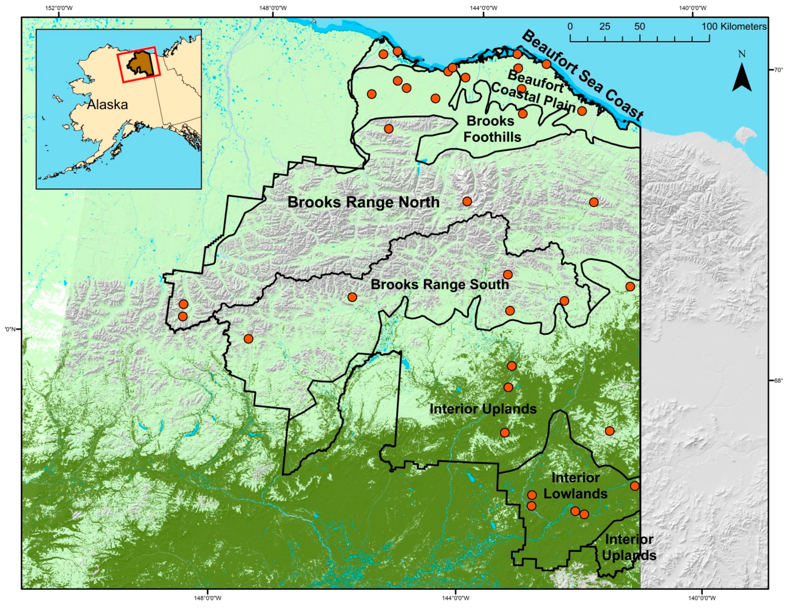
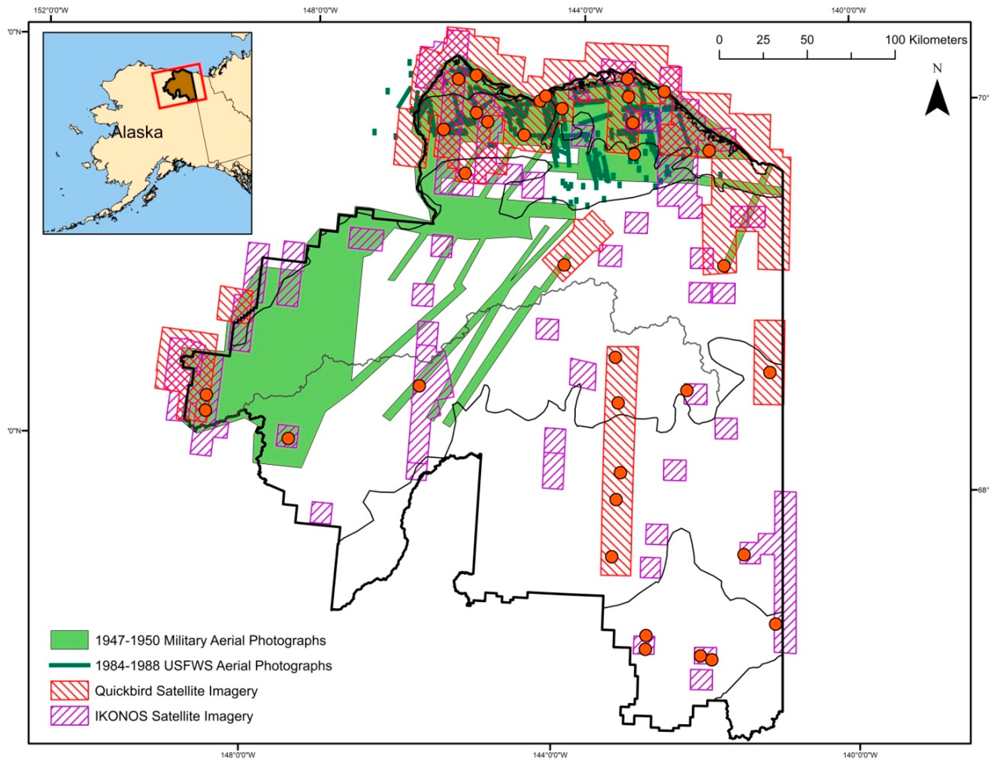
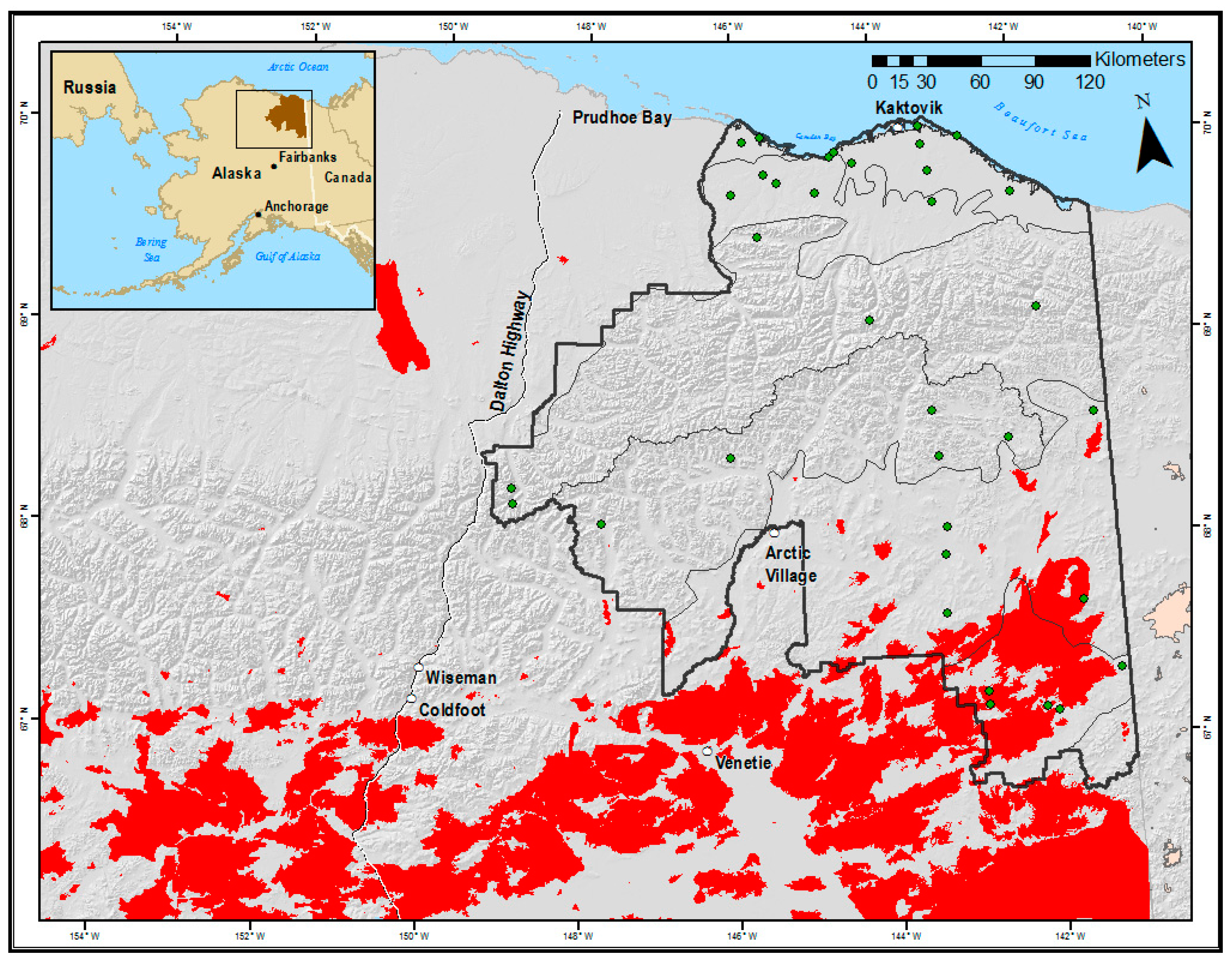
2.1. Study Area
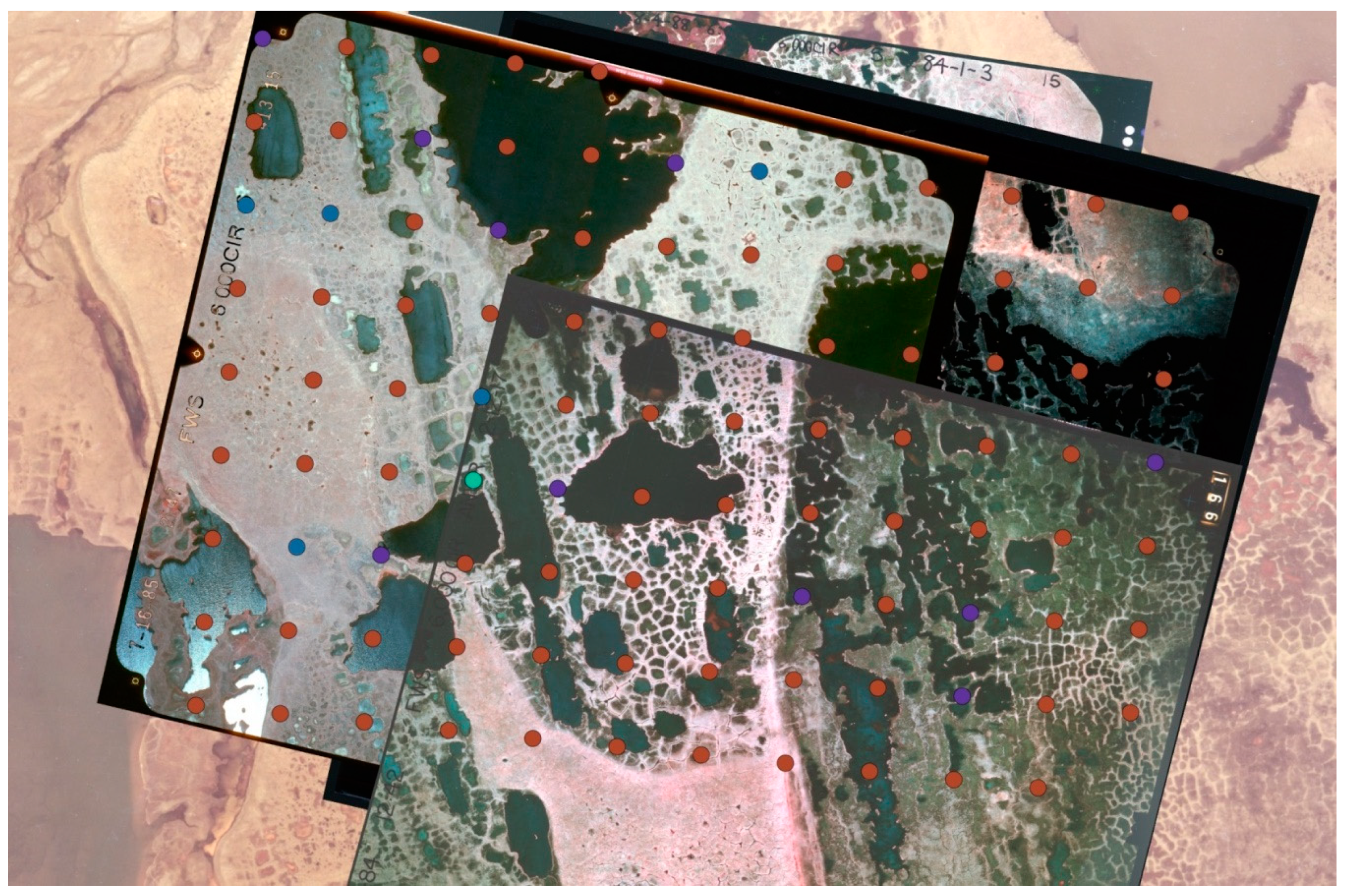
2.2. Sampling Design
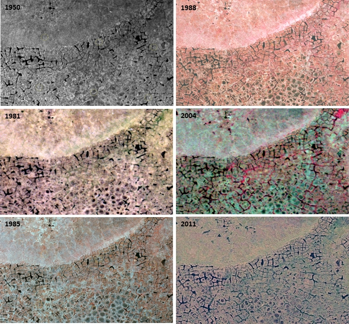
2.3. Image Acquisition and Manipulation
2.4. Image Interpretation
2.5. Environmental Variables
2.6. Data Analysis
3. Results
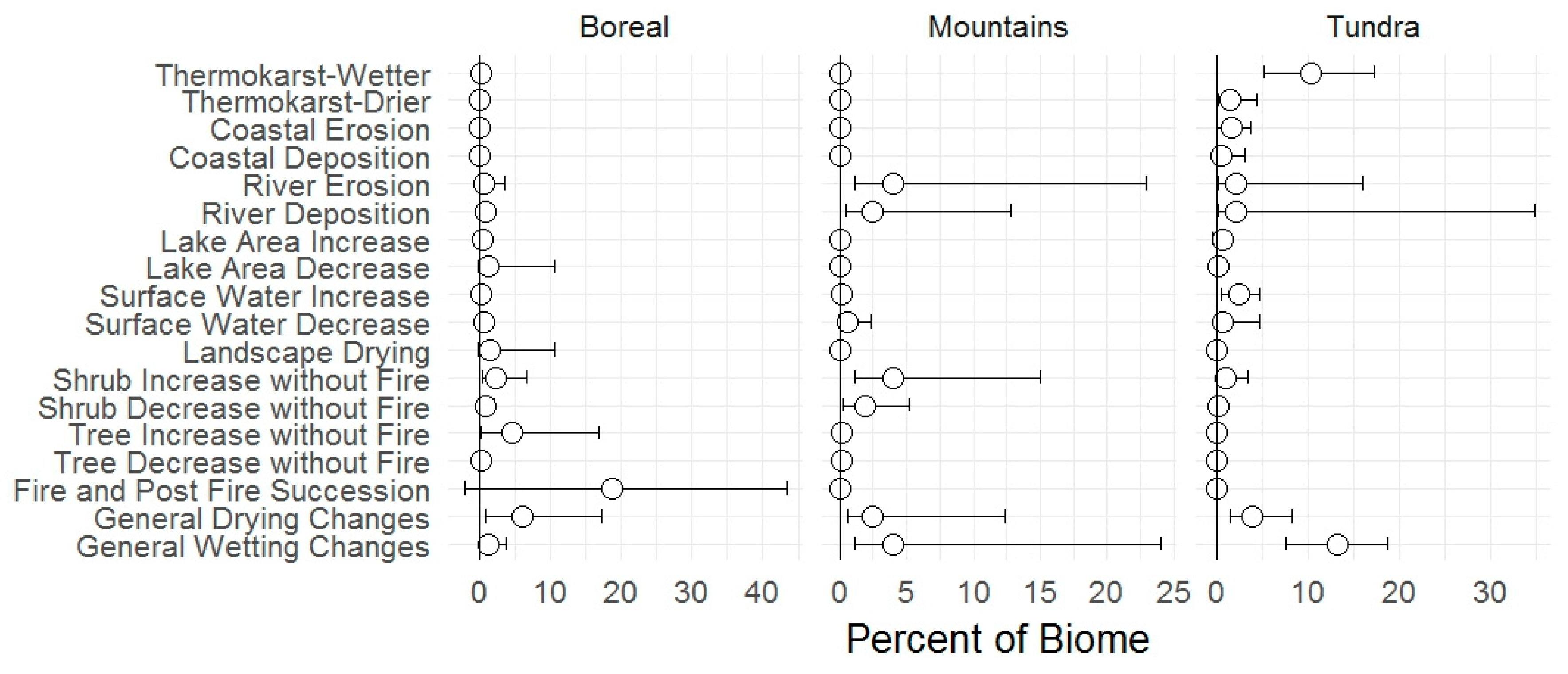
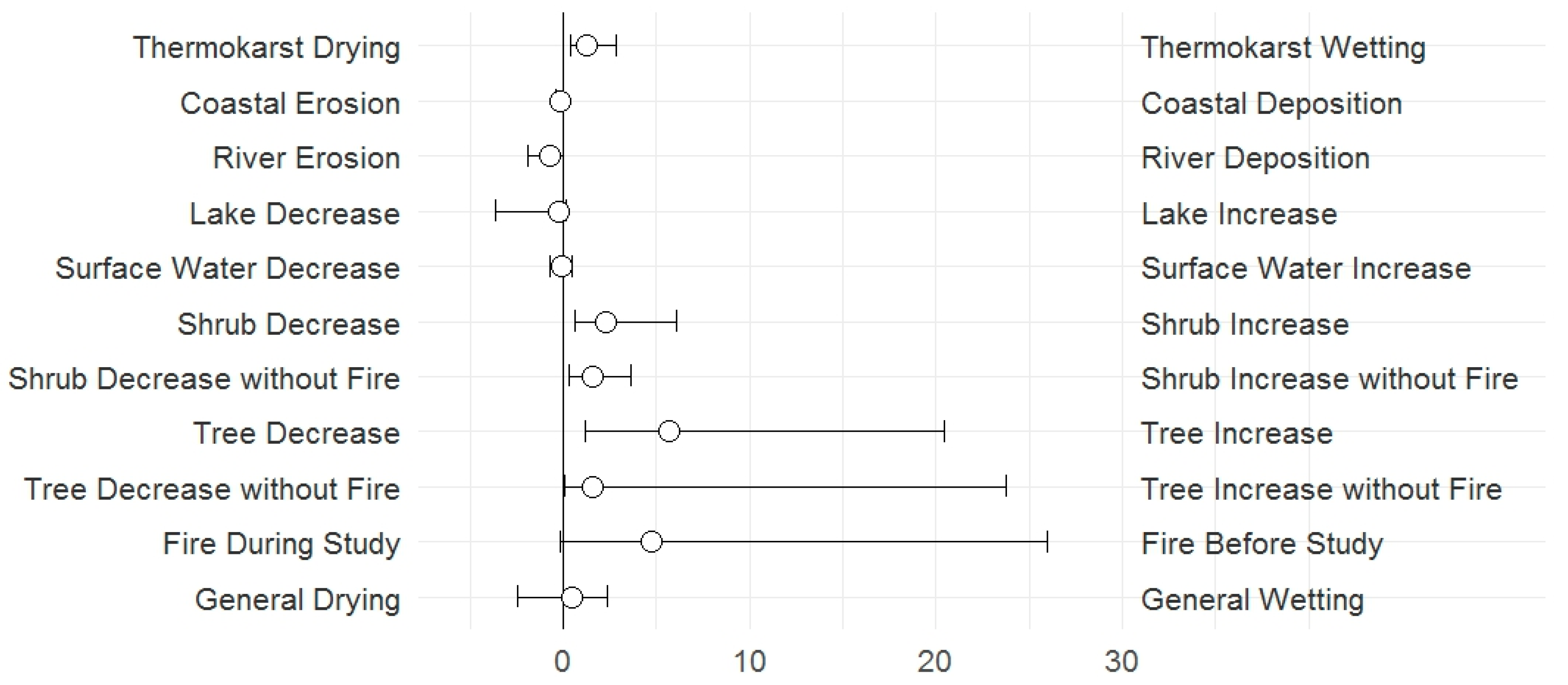
3.1. Change Types
3.2. Vegetation Types
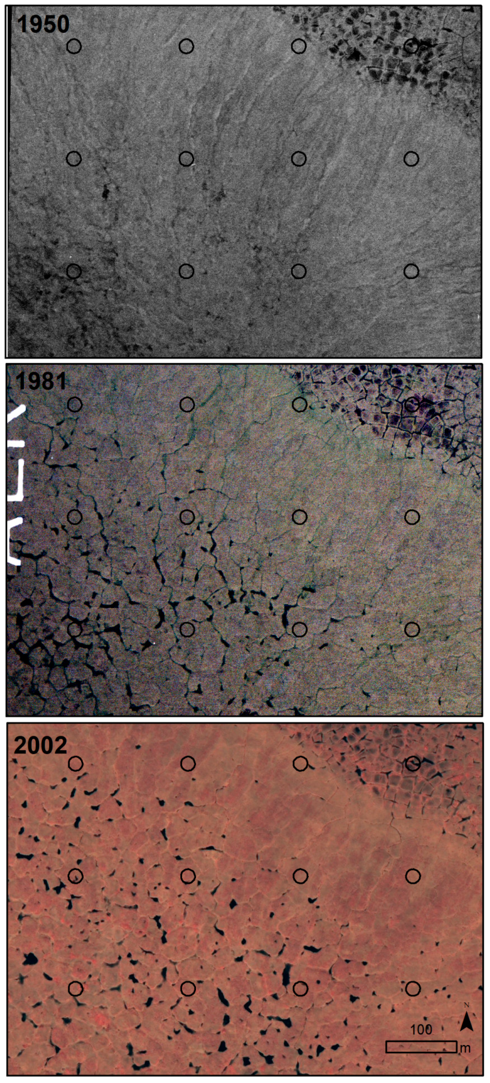
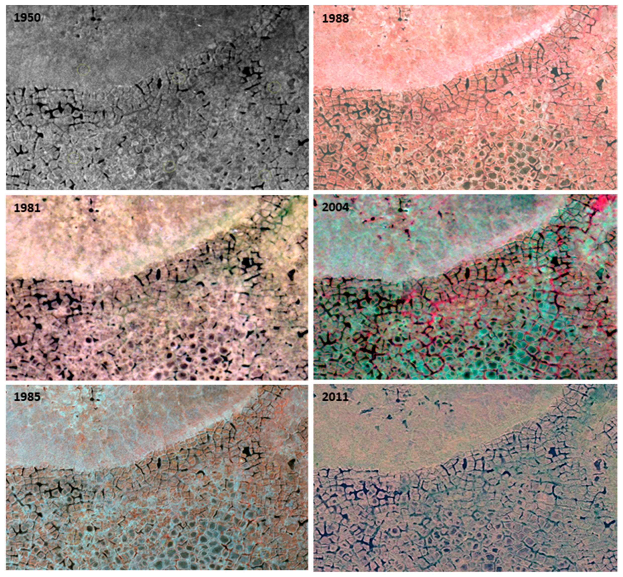
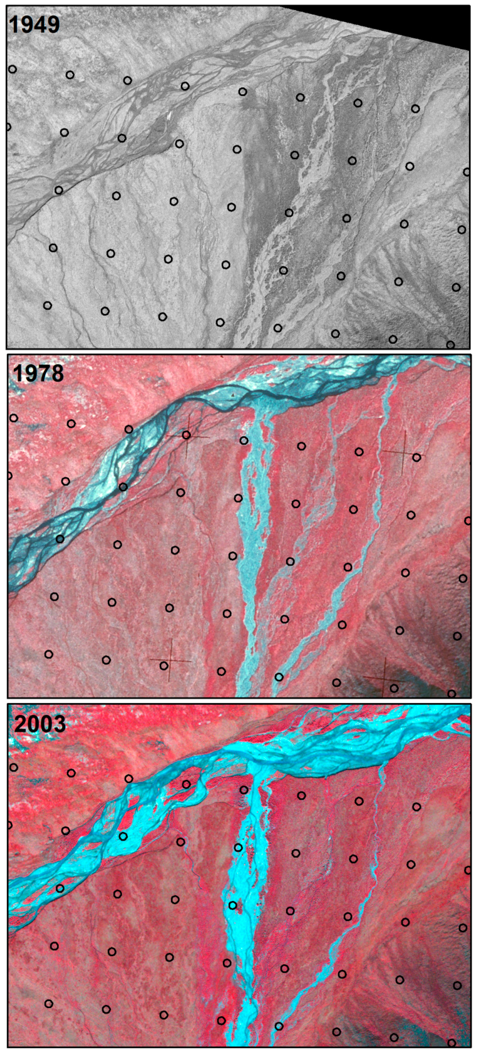
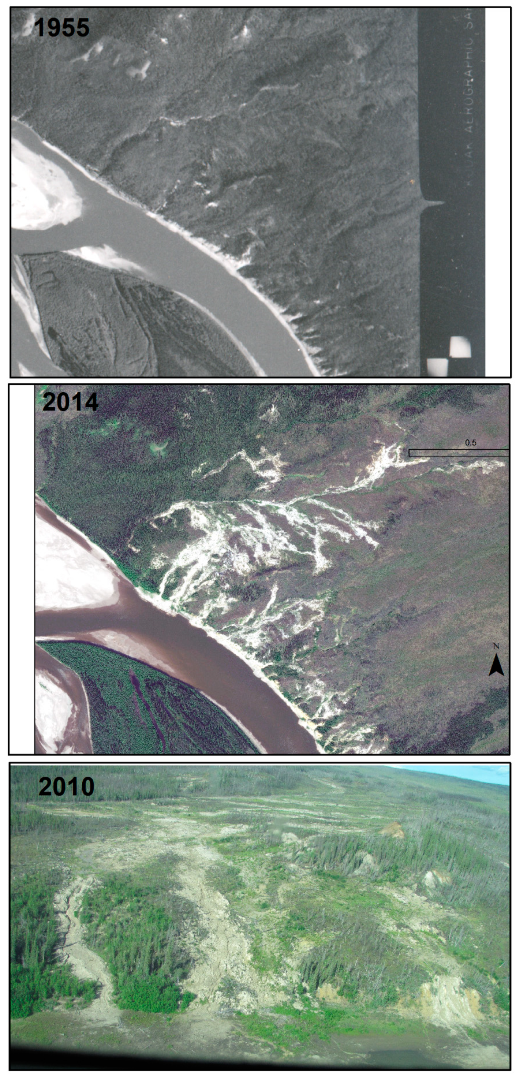
3.3. Changes Associated with Alluvial and Polygonal Terrain
4. Discussion
4.1. Change Types
4.2. Vegetation Types
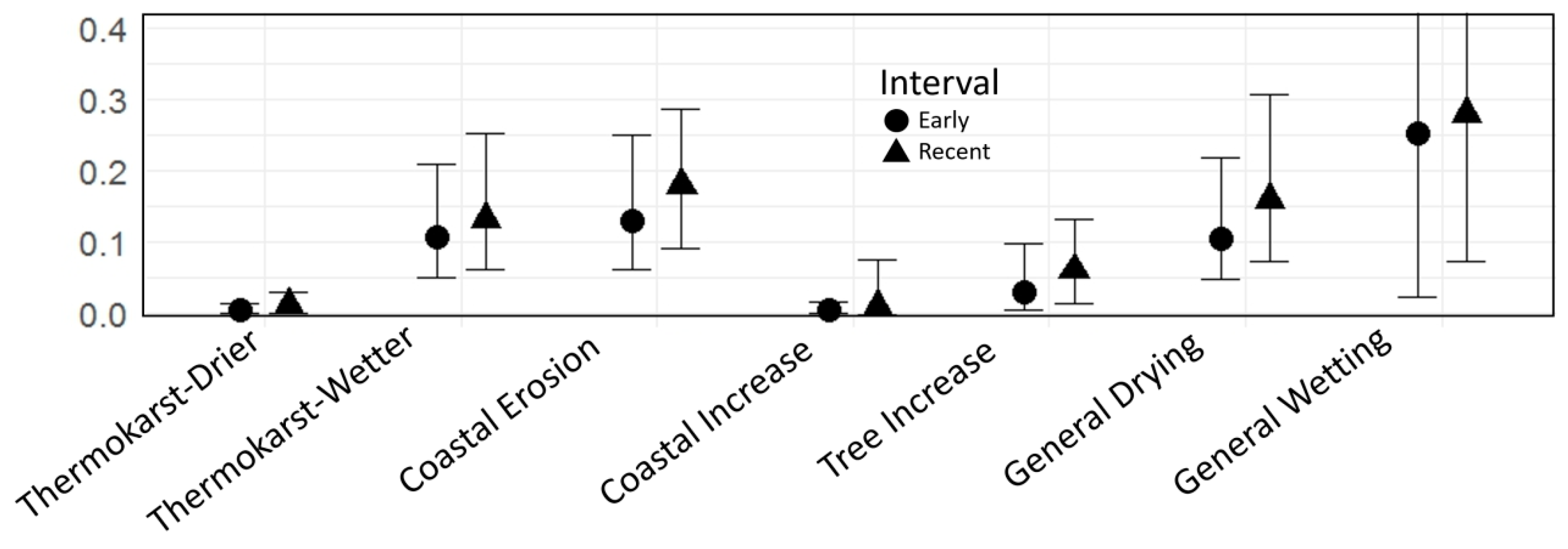
4.3. Rates of Change
4.4. Limitations and Applications of Remotely Sensed Change
5. Conclusions
Author Contributions
Funding
Acknowledgments
Conflicts of Interest
Appendix A


| Vegetation Type | Description |
|---|---|
| 1 FOREST | Trees >10% cover. Includes all trees even if temporarily low stature due to intermediate succession after fire or flooding. Includes open and closed canopy forest and woodlands. Understory has abundant shrubs, forbs, mosses and lichens. |
| 1.1 Spruce Forest | >60% of tree cover is needleleaf trees, mainly Picea glauca and also Picea mariana in most southern areas |
| 1.2 Mixed Forest | 40–60% each of spruce and broadleaf trees |
| 1.3 Broadleaf Forest | >60% of tree cover is broadleaf. Poplar (Populus balsamifera) mainly on floodplains, aspen (Populus tremuloides) and paper birch (Betula neoalaskana) mainly after fire. |
| 2 TALL SHRUB | Shrubs >1.5 m tall cover >25% of area. Includes open and closed canopies. Willows, mainly Salix alaxensis, and alder (Alnus viridis). |
| 2.1 Tall Riparian Shrub | Tall shrubs on river floodplains, banks of floodplains and narrow drainages. |
| 2.2 Tall Non-riparian Shrub | Non-floodplain, common in early and intermediate stages of post-fire succession |
| 3 LOW OR DWARF SHRUB | Shrubs <1.5 m tall cover >25% of area. |
| 3.1 Low Riparian Shrub | Shrubs 20–150 cm tall on river floodplains, banks of floodplains and narrow drainages. Mainly willows, e.g., Salix pulchra, S. richardsonii. |
| 3.2 Low Non-riparian Shrub | Shrubs 20–150 cm tall not on floodplains. Mainly the same willows above plus shrub birch (Betula glandulosa, B. nana) and other willows, e.g., S. glauca. |
| 3.3 Dwarf Shrub | Shrubs <20 cm tall. Mainly mountain avens (Dryas species, mainly D. integrifolia), dwarf willows (e.g., Salix reticulata), blueberry (Vaccinium uliginosum), cranberry (V. vitis-ideae), Labrador tea (Ledum groenlandicum, L. decumbens). On mountain slopes, late snow-melt areas, high-centered polygons and infrequently flooded river terraces. Many additional species in alpine areas. |
| 4 GRAMINOID | Graminoids predominate. The first 3 below also have high cover of mosses and dwarf and low shrubs. |
| 4.1 Tussock Tundra | Dominated by the tussock-forming sedge Eriophorum vaginatum. Includes shrubby tussock tundra, which may have >25% low shrub cover. |
| 4.2 Moist Sedge-Dryas Tundra | Dominated by sedges, usually Carex bigelowii, and the dwarf shrub Dryas integrifolia |
| 4.3 Moist Sedge-Willow Tundra | Dominated by sedges, usually Carex aquatilis and Eriophorum angustifolium, and willows, usually Salix pulchra. |
| 4.4 Wet Graminoid Tundra | Sedges, usually Carex aquatilis and Eriophorum angustifolium. Soil saturated throughout the growing season, so little willow or moss cover, except aquatic mosses. Some grass-dominated near the coast, e.g., Dupontia fisherii. |
| 4.5 Aquatic graminoid | Sedges and grasses in persistent standing water, mainly in shallow lakes |
| 4.6 Salt marsh | Coastal marshes with salt-tolerant species, mainly Carex subspathacea, Puccinellia spp. and Dupontia fisherii |
| 5 OTHER | Little cover of live plants, mainly on steep mountain slopes and active floodplains |
| 5.1 Sparsely Vegetated | 10–30% cover of vegetation |
| 5.2 Non-vegetated | 0–10% vegetation |
| 5.3 Water | <10% vegetation |
| Interpreted Change Type | Broad Change Type | Definition of Interpreted Type | # Points |
|---|---|---|---|
| 1 Fire: | Any change due to wildfire, even if the fire occurred before the study period | ||
| 1.1 Fire & post-fire succession | Fire & post-fire succession | Burned by wildfire, causing vegetation changes | 273 |
| 1.2 Fire, post-fire & thermokarst | Fire & post-fire succession | Burned, causing vegetation changes and ice wedge melting | 5 |
| 2 Ice-wedge degradation (Thermokarst): | Included only points with a change from one time period to the next, not all points with polygonal microtopography. Recorded for saltmarsh vs. other. | ||
| 2.1 Thermokarst-wetter | Thermokarst-wetter | Thermokarst with wetting effects within the circle. Increase in depth, width, or extent of ice-wedge polygon troughs, often with increase in water in troughs. | 130 |
| 2.2 Thermokarst-drier | Thermokarst-drier | Thermokarst with drying effects within the circle. Drying of troughs above ice wedges due to increased drainage of the general area as troughs enlarged, became more connected and allowed drainage. Or, graminoid cover increasing in troughs, accumulating dead leaves and causing less area and depth of surface water. Or, drying of polygon centers. | 22 |
| 3 River changes: | |||
| 3.1 River bank erosion | River erosion | Erosion into bank or uplands | 11 |
| 3.2 River erosion | River erosion | More river water in circle than in previous time period. River channel moving around on active floodplain, not into uplands. | 62 |
| 3.3 River deposition | River deposition | Less river water in circle than in previous time period. River channel moving around on active floodplain. | 61 |
| 4 Lake changes: | Recorded only if change in surface water detected within the 20-meter circle, not at points in centers of lakes | ||
| 4.1 Lake drying | Lake decrease | Lake became smaller and shallower. Water in circle disappeared. | 20 |
| 4.2 Lake drained | Lake decrease | Lake evidently drained all at once | 5 |
| 4.3 Lake accretion | Lake decrease | Sediment accreted along edge of lake, so less open water in circle | 1 |
| 4.4 Lake erosion | Lake increase | Lake eroded bank inside the circle, so more open water in circle | 9 |
| 4.5 Lake increase | Lake increase | Lake became larger. In circle, water covered previous land. | 5 |
| 5 Vegetation changes: | Recorded separately for post-fire changes vs. non-fire-related | ||
| 5.1 Shrub decrease | Shrub decrease | Decreased cover of shrubs | 26 |
| 5.2 Shrub increase | Shrub increase | Increased cover of shrubs | 83 |
| 5.3 Tree decrease | Tree decrease | Decreased cover of trees | 2 |
| 5.4 Tree increase | Tree increase | Increased cover of trees | 47 |
| 6 Coastal changes: | |||
| 6.1 Barrier erosion | Coastal erosion | Decreased area of off-shore barrier island in circle | 4 |
| 6.2 Coastal erosion | Coastal erosion | Erosion not including delta mud flat changes | 43 |
| 6.3 Salt marsh flooded | Coastal erosion | Within a salt marsh, increase in area of water and decrease in land in the circle | 2 |
| 6.4 Delta erosion | Coastal erosion | Decreased area of delta mud flats in circle (and increased area of sea) | 20 |
| 6.5 Barrier deposition | Coastal deposition | Increased area of barrier island in circle | 5 |
| 6.6 Coastal deposition | Coastal deposition | Deposition not including delta mud flats | 2 |
| 6.7 Delta deposition | Coastal deposition | Increased area of delta mud flats in circle | 10 |
| 6.8 Deposition in creek | Coastal deposition | Storm surge pushed beach gravels & logs into mouth of creek, forming pond | 1 |
| 6.9 Drift line move | Coastal - other | Driftwood line moved further inland over time, reaching to or beyond the point, indicating salt water intrusion | 4 |
| 6.10 Salt killed tundra | Coastal - other | Dead tundra vegetation, killed by salt water intrusion | 1 |
| 6.11 Sand deposition | Coastal - other | Sand deposition onto tundra from beach during storm surge | 1 |
| 6.12 Sand dune change | Coastal - other | Movement of sand dunes caused change in vegetation and sand cover | 5 |
| 7 Surface water change: | |||
| 7.1 Surface water increase | Surface water increase | Surface water, recorded at center of circle, absent in first year and present in last year | 45 |
| 7.2 Surface water decrease | Surface water decrease | Surface water, recorded at center of circle, present in first year and absent in last year | 22 |
| 8 Other: | |||
| 8.1 Land surface drying | Land surface drying | Drying of land surface, usually on abandoned floodplains near drying lake basins | 16 |
| 8.2 Scree fan increase | Scree fan increase | Scree at base of steep slope spread out over previously vegetated area | 2 |
| 8.3 Glacial retreat | Glacial retreat | Points on glacier in first 2 time periods and on bedrock outcrops protruding through the thinning glacier in last time period | 3 |
| 9. General drying or wetting: | Composite categories derived from some of the change types recorded | ||
| 9.1 General drying changes | General drying changes | Sum of points with drying changes: Less water at surface due to river deposition, lake or surface water decrease, thermokarst with drying, land surface drying or wildfire during the study period | 182 |
| 9.2 General wetting changes | General wetting changes | Sum of points with wetting changes: More water at surface due to river erosion, lake or surface water increase, or thermokarst with wetting | 236 |


References
- ACIA. Impacts of a Warming Arctic: Arctic Climate Impact Assessment; Cambridge University Press: Cambridge, UK, 2004; ISBN 0 521 61778 2. [Google Scholar]
- Parson, E.A.; Carter, L.; Anderson, P.; Wang, B.; Weller, G.; Maccracken, M. Potential consequences of climate variability and change for Alaska. In Climate Change Impacts on the United States; Parson, E.A., Carter, L., Anderson, P., Wang, B., Weller, G., Maccracken, M., Eds.; U.S. Global Change Research Program: Washington, DC, USA, 2001; pp. 283–312. ISBN 0521000750. [Google Scholar]
- Mantua, N.J.; Hare, S.R. The Pacific Decadal Oscillation. J. Oceanogr. 2002, 58, 35–44. [Google Scholar] [CrossRef]
- Hartmann, B.; Wendler, G. The significance of the 1976 Pacific climate shift in the climatology of Alaska. J. Clim. 2005, 18, 4824–4839. [Google Scholar] [CrossRef]
- Hinzman, L.; Bettez, N.; Bolton, B.; Chapin, F.S.; Dyurgerov, M.B.; Fastie, C.L.; Griffith, B.; Hollister, R.D.; Hope, A.; Huntington, H.P.; et al. Evidence and implications of recent climate change in terrestrial regions of the Arctic. Clim. Chang. 2005, 72, 251–298. [Google Scholar] [CrossRef]
- Hinzman, L.D.; Deal, C.J.; McGuire, A.D.; Mernild, S.H.; Polyakov, I.V.; Walsh, J.E. Trajectory of the Arctic as an integrated system. Ecol. Appl. 2013, 23, 1837–1868. [Google Scholar] [CrossRef] [PubMed]
- Gogineni, P.; Romanovsky, V.; Cherry, J.; Duguay, C.; Goetz, S.; Jorgenson, M.T.; Moghaddami, M. Opportunities to Use Remote Sensing in Understanding Permafrost and Related Ecological Characteristics: Report of a Workshop; National Academy of Science: Washington, DC, USA, 2014; p. 84. ISBN 978-0-309-30121-3. [Google Scholar]
- Jorgenson, M.T.; Grosse, G. Remote sensing of landscape change in permafrost regions. Permafr. Periglac. Processes 2016, 27, 324–338. [Google Scholar] [CrossRef]
- Bhatt, U.S.; Walker, D.A.; Raynolds, M.K.; Comiso, J.C.; Epstein, H.E.; Jia, G.; Gens, R.; Tweedie, C.E.; Tucker, C.J.; Webber, P.J. Circumpolar arctic tundra vegetation change is linked to sea ice decline. Earth Interact. 2010, 14, 1–20. [Google Scholar] [CrossRef]
- Beck, P.S.A.; Goetz, S.J. Satellite observations of high northern latitude vegetation productivity changes between 1982 and 2008: Ecological variability and regional differences. Environ. Res. Lett. 2011, 6, 045501. [Google Scholar] [CrossRef]
- Epstein, H.E.; Raynolds, M.K.; Walker, D.A.; Bhatt, U.S.; Tucker, C.J.; Pinzon, J.E. Dynamics of aboveground phytomass of the circumpolar arctic tundra over the past three decades. Environ. Res. Lett. 2012, 7, 015506. [Google Scholar] [CrossRef]
- Jia, G.J.; Epstein, H.E.; Walker, D.A. Greening of arctic Alaska, 1981–2001. Geophys. Res. Lett. 2003, 30, 2067. [Google Scholar] [CrossRef]
- Stow, D.A.; Hope, A.; Mcguire, D.; Verbyla, D.; Gamon, J.; Huemmrich, F.; Houston, S.; Racine, C.; Sturm, M.; Tape, K.; et al. Remote sensing of vegetation and land-cover change in arctic tundra ecosystems. Remote Sens. Environ. 2004, 89, 281–308. [Google Scholar] [CrossRef]
- Frost, G.V.; Epstein, H.E. Tall shrub and tree expansion in Siberian tundra ecotones since the 1960s. Glob. Chang. Biol. 2014, 20, 1264–1277. [Google Scholar] [CrossRef] [PubMed]
- Myers-Smith, I.H.; Forbes, B.C.; Wilmking, M.; Hallinger, M.; Lantz, T.C.; Block, D.; Tape, K.D.; Macias-Fauria, M.; Sass-Klaassen, U.; Lévesque, E. Shrub expansion in tundra ecosystems: Dynamics, impacts and research priorities. Environ. Res. Lett. 2011, 6, 045509. [Google Scholar] [CrossRef]
- Bhatt, U.S.; Walker, D.A.; Raynolds, M.K.; Bieniek, P.A.; Epstein, H.E.; Comiso, J.C.; Pinzon, J.E.; Tucker, C.J.; Polyakov, I.V. Recent declines in warming and arctic vegetation greening trends over pan-arctic tundra. Remote Sens. 2013, 5, 4229–4254. [Google Scholar] [CrossRef]
- Pattison, R.; Jorgenson, J.C.; Raynolds, M.K.; Welker, J. Trends in NDVI and tundra community composition in the arctic of NE Alaska between 1984 to 2009. Ecosystems 2015, 18, 707–719. [Google Scholar] [CrossRef]
- Raynolds, M.K.; Walker, D.A.; Verbyla, D.; Munger, C.A. Patterns of change within a tundra landscape: 22-year landsat ndvi trends in an area of the northern foothills of the Brooks Range, Alaska. Arct. Antarct. Alp. Res. 2013, 45, 249–260. [Google Scholar] [CrossRef]
- Elmendorf, S.C.; Henry, G.H.R.; Hollister, R.D.; Bjork, R.G.; Boulanger-Lapointe, N.; Cooper, E.J.; Cornelissen, J.H.C.; Day, T.A.; Dorrepaal, E.; Elumeeva, T.G.; et al. Plot-scale evidence of tundra vegetation change and links to recent summer warming. Nat. Clim. Chang. 2012, 2, 453–457. [Google Scholar] [CrossRef]
- Jorgenson, J.C.; Raynolds, M.K.; Reynolds, J.H.; Benson, A.M. Twenty-five year record of changes in plant cover on tundra of northeastern Alaska. Arct. Antarct. Alp. Res. 2015, 47, 785–806. [Google Scholar] [CrossRef]
- Jorgenson, M.T.; Shur, Y.L.; Pullman, E.R. Abrupt increase in permafrost degradation in arctic Alaska. Geophys. Res. Lett. 2006, 33, L02503. [Google Scholar] [CrossRef]
- Johnstone, J.F.; Chapin, F.S., III; Hollingsworth, T.N.; Mack, M.C.; Romanovsky, V.; Turetsky, M. Fire, climate change, and forest resilience in interior Alaska. Can. J. For. Res. 2010, 40, 1302–1312. [Google Scholar] [CrossRef]
- Kasischke, E.S.; Verbyla, D.L.; Rupp, T.S.; McGuire, A.D.; Murphy, K.A.; Jandt, R.; Barnes, J.L.; Hoy, E.E.; Duffy, P.A.; Calef, M.; et al. Alaska’s changing fire regime—Implications for the vulnerability of its boreal forests. Can. J. For. Res. 2010, 40, 1313–1324. [Google Scholar] [CrossRef]
- Riordan, B.; Verbyla, D.; McGuire, A.D. Shrinking ponds in subarctic Alaska based on 1950–2002 remotely sensed images. J. Geophys. Res. 2006, 111, G04002. [Google Scholar] [CrossRef]
- Jones, B.M.; Grosse, G.; Arp, C.D.; Jones, M.C.; Walter Anthony, K.M.; Romanovsky, V.E. Modern thermokarst lake dynamics in the continuous permafrost zone, northern Seward Peninsula, Alaska. J. Geophys. Res. Biogeosci. 2011, 116, G00M03. [Google Scholar] [CrossRef]
- Tape, K.; Sturm, M.; Racine, C. The evidence for shrub expansion in northern Alaska and the pan-arctic. Glob. Chang. Biol. 2006, 12, 686–702. [Google Scholar] [CrossRef]
- Swanson, D.K. Three Decades of Landscape Change in Alaska’s Arctic National Parks: Analysis of Aerial Photographs C. 1980–2010; National Park Service: Fort Collins, CO, USA, 2014; p. 29. Available online: https://www.sciencebase.gov/ catalog/item/5771b8e2e4b07657d1a6d812 (accessed on 8 May 2018).
- Naito, A.T.; Cairns, D.M. Patterns of shrub expansion in Alaskan arctic river corridors suggest phase transition. Ecol. Evol. 2015, 5, 87–101. [Google Scholar] [CrossRef] [PubMed]
- Jorgenson, M.T.; Racine, C.H.; Walters, J.C.; Osterkamp, T.E. Permafrost degradation and ecological changes associated with a warming climate in central Alaska. Clim. Chang. 2001, 48, 551–579. [Google Scholar] [CrossRef]
- Jorgenson, M.T.; Kanevksiy, M.Z.; Shur, Y.; Wickland, K.; Nossov, D.R.; Moskalenko, N.G.; Koch, J.; Striegl, R. Role of ground-ice dynamics and ecological feedbacks in recent ice-wedge degradation and stabilization. J. Geophys. Res. Earth Surf. 2015, 120, 2280–2297. [Google Scholar] [CrossRef]
- Swanson, D.K. Mapping of Erosion Features Related to Thaw of Permafrost in Bering Land Bridge National Preserve, Cape Krusenstern National Monument, and Kobuk National Park; National Park Service: Fort Collins, CO, USA, 2010; p. 18. Available online: https://irma.nps.gov/DataStore/DownloadFile/446412 (accessed on 8 May 2018).
- Shulski, M.; Wendler, G. The Climate of Alaska; University of Alaska Press: Fairbanks, AK, USA, 2007; ISBN 978-1602230071. [Google Scholar]
- Jorgenson, J.C.; Joria, P.C.; Douglas, D.C. Section 3: Land Cover; Vol. Biological Science Report USGS/BRD/BSR-2002-0001; U.S. Geological Survey: Reston, VA, USA, 2002; pp. 4–7.
- Nowacki, G.; Spencer, P.; Brock, T.; Fleming, M.; Jorgenson, T. Ecoregions of Alaska and Neighboring Territories; U.S. Geological Survey: Washington, DC, USA, 2001. Available online: https://agdc.usgs.gov/data/usgs/erosafo/ecoreg/index.html (accessed on 8 May 2018).
- Viereck, L.A.; Dyrness, C.T.; Batten, A.R.; Wenzlick, K.J. The Alaska Vegetation Classification. Pacific Northwest Research Station; Vol. Gen. Tech. Rep. PNW-GTR-286; U.S. Forest Service: Portland, OR, USA, 1992; p. 278. Available online: https://www.fs.fed.us/pnw/publications/pnw_gtr286/pnw_gtr286a.pdf (accessed on 8 May 2018).
- Jorgenson, M.T.; Grunblatt, J. Landscape-Level Ecological Mapping of Northern Alaska and Field Site Photography; Final Report prepared for Arctic Land Conservation Cooperative by Alaska Ecoscience, Fairbanks, AK, USA, and Geographic Information Network of Alaska; University of Alaska Fairbanks: Fairbanks, AK, USA, 2013; p. 48. Available online: https://lccnetwork.org/resource/ landscape-level-ecological-mapping-northern-alaska-and-field-site-photography-report (accessed on 8 May 2018).
- Pastick, N.J.; Wylie, B.K.; Jorgenson, M.T.; Goetz, S.J.; Jones, B.M.; Swanson, D.K.; Minsley, B.J.; Genet, H.; Knight, J.F.; Jorgenson, J.C. Spatiotemporal remote sensing of ecosystem change and causation across Alaska. Glob. Chang. Biol. 2018, 1–19. [Google Scholar] [CrossRef] [PubMed]
- Kasischke, E.S.; Turetsky, M.R. Recent changes in the fire regime across the North American boreal region—Spatial and temporal patterns of burning across Canada and Alaska. Geophys. Res. Lett. 2006, 33, L09703. [Google Scholar] [CrossRef]
- Jones, B.M.; Breen, A.L.; Gaglioti, B.V.; Mann, D.H.; Rocha, A.V.; Grosse, G.; Walker, D.A. Identification of unrecognized tundra fire events on the north slope of Alaska. J. Geophys. Res. Biogeosci. 2013, 118, 1334–1344. [Google Scholar] [CrossRef] [Green Version]
- Jones, B.M.; Kolden, C.A.; Jandt, R.; Abatzoglou, J.T.; Urban, F.; Arp, C.D. Fire behavior, weather, and burn severity of the 2007 Anaktuvuk River tundra fire, North Slope, Alaska. Arct. Antarct. Alp. Res. 2009, 41, 309–316. [Google Scholar] [CrossRef]
- Jones, B.M.; Grosse, G.; Arp, C.D.; Liu, L.; Miller, E.A.; Hayes, D.J.; Larsen, C. Recent arctic tundra fire initiates widespread thermokarst development. Sci. Rep. 2015, 5, 15865. [Google Scholar] [CrossRef] [PubMed] [Green Version]
- Brown, D.; Jorgenson, M.T.; Kielland, K.; Verbyla, D.L.; Prakash, A.; Koch, J.C. Landscape effects of wildfire on permafrost distribution in interior Alaska derived from remote sensing. Remote Sens. 2016, 8, 654. [Google Scholar] [CrossRef]
- Nolan, M.; Arendt, A.; Rabus, B.; Hinzman, L. Volume change of McCall glacier, arctic Alaska, USA, 1956–2003. Ann. Glaciol. 2005, 42, 409–416. [Google Scholar] [CrossRef]
- Epstein, H.E.; Myers-Smith, I.; Walker, D.A. Recent dynamics of arctic and sub-arctic vegetation. Environ. Res. Lett. 2013, 8, 015040. [Google Scholar] [CrossRef] [Green Version]
- Swanson, D.K. Environmental limits of tall shrubs in Alaska’s arctic national parks. PLoS ONE 2015, 10, e0138387. [Google Scholar] [CrossRef] [PubMed]
- Tape, K.; Verbyla, D.; Welker, J. 20th century erosion in arctic Alaska foothills: The influence of shrubs, runoff, and permafrost. J. Geophys. Res. Biogeosci. 2011, 116, G04024. [Google Scholar] [CrossRef]
- U.S. Boundary Commission. Alaska-Canada Boundary Survey Map Set; U.S. Geological Survey: Washington, DC, USA, 2011.
- Harsch, M.A.; Hulme, P.E.; McGlone, M.S.; Duncan, R.P. Are treelines advancing? A global meta-analysis of treeline response to climate warming. Ecol. Lett. 2009, 12, 1040–1049. [Google Scholar] [CrossRef] [PubMed]
- Liljedahl, A.K.; Boike, J.; Daanen, R.P.; Fedorov, A.N.; Frost, G.V.; Grosse, G.; Larry, D.H.; Yoshihiro, I.; Janet, C.J.; Nadya, M.; et al. Pan-arctic ice-wedge degradation in warming permafrost and its influence on tundra hydrology. Nat. Geosci. 2016, 9, 312–318. [Google Scholar] [CrossRef]
- Swanson, D.K. Permafrost landforms as indicators of climate change in the arctic network of national parks. Alaska Park Sci. 2013, 12, 40–45. [Google Scholar]
- Farquharson, L.M.; Mann, D.H.; Grosse, G.; Jones, B.M.; Romanovsky, V.E. Spatial distribution of thermokarst terrain in arctic Alaska. Geomorphology 2016, 273, 116–133. [Google Scholar] [CrossRef]
- Jorgenson, M.T.; Shur, Y.L.; Osterkamp, T.E. Thermokarst in Alaska. In Proceedings of the Ninth International Conference on Permafrost, Fairbanks, AK, USA, June 29–July 3 2008; Kane, D.L., Hinkel, K.M., Eds.; Institute of Northern Engineering; University of Alaska: Fairbanks, AK, USA, 2008; pp. 869–876. ISBN 978-0-9800179-2-2. [Google Scholar]
- Jorgenson, M.T.; Harden, J.; Kanevskiy, M.; O’Donnel, J.; Wickland, K.; Ewing, S.; Manies, K.; Zhuang, Q.; Shur, Y.; Striegl, R.; et al. Reorganization of vegetation, hydrology and soil carbon after permafrost degradation across heterogeneous boreal landscapes. Environ. Res. Lett. 2013, 8, 035017. [Google Scholar] [CrossRef] [Green Version]
- Swanson, D.K. Mapping of Erosion Features Related to Thaw of Permafrost in the Noatak National Preserve, Alaska; National Park Service: Fort Collins, CO, USA, 2012; p. 28. Available online: https://irma.nps.gov/DataStore/DownloadFile/446412 (accessed on 8 May 2018).
- Jorgenson, M.T.; Brown, J. Classification of the Alaskan Beaufort Sea coast and estimation of sediment and carbon inputs from coastal erosion. GeoMarine 2005, 482, 32–45. [Google Scholar] [CrossRef] [Green Version]
- Jorgenson, M.T.; Jorgenson, J.C.; Macander, M.; Payer, D.; Morkill, A.E. Monitoring of Coastal Dynamics at Beaufort Lagoon in the Arctic National Wildlife Refuge, Northeast Alaska; Reports on Polar and Marine Research, Arctic Coastal Dynamics Report of an International Workshop, Potsdam, Germany, 26–30 November 2001. Available online: http://rep4-vm.awi.de/26592/1/BerPolarforsch2002413.pdf#page=28 (accessed on 8 May 2018).
- Jones, B.M.; Arp, C.D.; Jorgenson, M.T.; Hinkel, K.M.; Schmutz, J.A.; Flint, P.L. Increase in the rate and uniformity of coastline erosion in arctic Alaska. Geophys. Res. Lett. 2009, 36, L03503. [Google Scholar] [CrossRef]
- Roach, J.; Griffith, B.; Verbyla, D. Landscape influences on climate-related lake shrinkage at high latitudes. Glob. Chang. Biol. 2013, 19, 2276–2284. [Google Scholar] [CrossRef] [PubMed]
- Necsoiu, M.; Dinwiddie, C.L.; Walter, G.R.; Larsen, A.; Stothoff, S.A. Multi-temporal image analysis of historical aerial photographs and recent satellite imagery reveals evolution of water body surface area and polygonal terrain morphology in Kobuk Valley National Park, Alaska. Environ. Res. Lett. 2013, 8, 16. [Google Scholar] [CrossRef]
- Plug, L.J.; Walls, C.; Scott, B.M. Thermokarst lake changes from 1978–2001 on the Tuktoyaktuk Peninsula, western Canadian Arctic. Geophys. Res. Lett. 2008, 35, L03502. [Google Scholar] [CrossRef]
- Pavelsky, T.M.; Zarnetske, J.P. Rapid decline in river icings detected in arctic Alaska: Implications for a changing hydrologic cycle and river ecosystems. Geophys. Res. Lett. 2017, 44, 3228–3235. [Google Scholar] [CrossRef]
- Jorgenson, M.T.; Marcot, B.G.; Swanson, D.K.; Jorgenson, J.C.; DeGange, A.R. Projected changes in diverse ecosystems from climate warming and biophysical drivers in northwest Alaska. Clim. Chang. 2015, 130, 131–144. [Google Scholar] [CrossRef] [Green Version]
- Sormunen, H.; Virtanen, R.; Luoto, M. Inclusion of local environmental conditions alters high-latitude vegetation change predictions based on bioclimatic models. Polar Biol. 2011, 34, 883–897. [Google Scholar] [CrossRef]


| Biomes & Ecoregions (North to South) | % of Refuge | Area (km2) | % Burned (1950–2010) | Mean Annual Temp. (oC) | January Temp. (oC) | July Temp (oC) | Mean Elevation (m) | Mean Slope (o) |
|---|---|---|---|---|---|---|---|---|
| Tundra Biome: | ||||||||
| Beaufort Sea Coast | 1 | 850 | 0 | −11 | −26 | 6 | 3 | 1 |
| Beaufort Coastal Plain | 5 | 3788 | 0 | −11 | −26 | 6 | 59 | 1 |
| Brooks Foothills | 8 | 6278 | 0 | −10 | −26 | 9 | 317 | 3 |
| Mountain Biome: | ||||||||
| Brooks Range North | 31 | 24,731 | 0 | −8 | −25 | 9 | 1106 | 22 |
| Brooks Range South | 21 | 16,488 | 0 | −8 | −26 | 10 | 1170 | 18 |
| Boreal Biome: | ||||||||
| Interior Uplands | 27 | 22,064 | 12 | −6 | −24 | 14 | 633 | 5 |
| Interior Lowlands | 8 | 6126 | 58 | −5 | −26 | 15 | 350 | 3 |
| Whole Refuge | 100 | 80,325 | 8 | −8 | −25 | 11 | 813 | 13 |
| Image Type | Source | Dates | Color | Scale | Resolution (m) |
|---|---|---|---|---|---|
| Aerial Photography | U. S. Air Force | 1947 | B & W | 1:40,000, 1:30,000, 1:12,000 | 0.3–1.0 |
| Aerial Photography | Naval Arctic Research Laboratory | 1948–1950 | B & W | 1:20,000 | 0.4–0.6 |
| Aerial Photography | U. S. Geological Survey | 1955 | B & W | 1:50,000 | 1.0 |
| Aerial Photography | Alaska High-Altitude Photography Program | 1978–1982 | Color Infrared | 1:60,000 | 1.0 |
| Aerial Photography | U. S. Fish & Wildlife Service | 1981 | True Color | 1:18,000 | 0.3 |
| Aerial Photography | U. S. Fish & Wildlife Service | 1984, 1985, 1988 | Color Infrared | 1:6,000 | 0.1 |
| Quickbird Satellite Imagery | Digital Globe | 2002–2007 | Color (pan-sharpened) & B&W (pan) | 0.6 (pan), 2.4 (color) | |
| IKONOS Satellite Imagery | Digital Globe | 2000–2006 | Color (pan-sharpened) & B&W (pan) | 0.8 (pan), 4 (color) | |
| Worldview Satellite Imagery | Digital Globe | 2010–2015 | True Color (pan-sharpened) | 0.3 |
| Landscape Change | BIOMES | Whole Refuge | |||||||||
|---|---|---|---|---|---|---|---|---|---|---|---|
| Boreal | Mountains | North Slope Tundra | |||||||||
| Interior Lowlands | Interior Uplands | Whole Biome | South Side | North Side | Whole Biome | Brooks Foothills | Coastal Plain | Coastal Marine | Whole Biome | ||
| Fire & post-fire succession | 45 | 11 | 18 | 0 | 0 | 0 | 0 | 0 | 0 | 0 | 6 |
| Thermokarst wetting | 1 | 0 | <1 | 0 | 0 | 0 | 10 | 12 | 7 | 10 | 1 |
| Thermokarst drying | <1 | 0 | 0 | 0 | 0 | 0 | 1 | 2 | 2 | 2 | <1 |
| Vegetation change without fire: | |||||||||||
| Tree increase | 4 | 5 | 5 | <1 | 0 | <1 | 0 | 0 | 0 | 0 | 2 |
| Tree decrease | 0 | <1 | <1 | <1 | 0 | <1 | 0 | 0 | 0 | 0 | <1 |
| Shrub increase | 5 | 1 | 2 | 4 | 6 | 6 | 1 | 1 | 0 | 1 | 4 |
| Shrub decrease | 0 | 1 | 1 | 2 | 2 | 2 | <1 | 0 | 0 | <1 | <1 |
| River erosion | <1 | 1 | 1 | 4 | 4 | 4 | 1 | 4 | 1 | 2 | 3 |
| River deposition | 0 | 1 | 1 | 3 | 2 | 2 | 1 | 5 | <1 | 2 | 2 |
| Lake decrease | 4 | <1 | 1 | 0 | 0 | 0 | 0 | <1 | 1 | <1 | <1 |
| Lake increase | 1 | <1 | <1 | 0 | 0 | 0 | 0 | 2 | 0 | 1 | <1 |
| Coastal erosion | 0 | 0 | 0 | 0 | 0 | 0 | 0 | 0 | 18 | 2 | <1 |
| Coastal deposition | 0 | 0 | 0 | 0 | 0 | 0 | 0 | 0 | 5 | 1 | <1 |
| Coastal storm surges & dunes | 0 | 0 | 0 | 0 | 0 | 0 | 0 | 0 | 2 | <1 | <1 |
| Landscape drying | 2 | 1 | 2 | 0 | 0 | 0 | 0 | 0 | 0 | 0 | <1 |
| Glacial retreat | 0 | 0 | 0 | 0 | 1 | <1 | 0 | 0 | 0 | 0 | <1 |
| Scree slides | 0 | 0 | 0 | <1 | <1 | <1 | 0 | 0 | 0 | 0 | <1 |
| % with change of any type | 58 | 20 | 28 | 9 | 11 | 10 | 14 | 24 | 36 | 19 | 18 |
| Vegetation Types | % of Whole Arctic Refuge | % of Tundra Biome | % of Mountain Biome | % of Boreal Biome | Most Common Change Detected in This Vegetation Type | % with Any Change |
|---|---|---|---|---|---|---|
| FOREST | 19 | 0 | 2 | 52 | Fire & post-fire succession | 39 |
| Spruce Forest | 9 | 0 | 2 | 21 | Fire & post-fire succession | 31 |
| Mixed Forest | 8 | 0 | 0 | 25 | Fire & post-fire succession | 39 |
| Broadleaf Forest | 2 | 0 | 0 | 6 | Fire & post-fire succession | 77 |
| TALL SHRUB | 5 | 0 | 5 | 9 | Shrub increase, with or without fire | 44 |
| Tall Riparian Shrub | 2 | 0 | 3 | 1 | River erosion & shrub increase (without fire) | 53 |
| Tall Non-riparian Shrub | 3 | 0 | 2 | 8 | Fire & post-fire succession | 38 |
| LOW OR DWARF SHRUB | 28 | 12 | 40 | 21 | Fire & post-fire succession | 19 |
| Low Riparian Shrub | 3 | 1 | 4 | 1 | River erosion | 32 |
| Low Non-riparian Shrub | 14 | 10 | 15 | 20 | Fire & post-fire succession | 26 |
| Dwarf Shrub | 11 | 1 | 21 | <1 | Shrub increase (without fire) | 7 |
| GRAMINOID | 22 | 77 | 9 | 15 | Thermokarst-wetting | 16 |
| Tussock Tundra | 6 | 19 | 4 | 4 | Thermokarst-wetting | 5 |
| Moist Sedge-Dryas Tundra | 6 | 25 | 2 | 3 | Thermokarst-wetting | 24 |
| Moist Sedge-Willow Tundra | 4 | 15 | 2 | 3 | Thermokarst-wetting | 14 |
| Wet Graminoid Tundra | 5 | 15 | 1 | 7 | Thermokarst-wetting | 16 |
| Salt marsh and Aquatic | <1 | 3 | 0 | <1 | Thermokarst-wetting & coastal erosion | 27 |
| OTHER | 26 | 11 | 43 | 3 | River erosion & deposition | 20 |
| Sparsely Vegetated | 6 | 1 | 11 | <1 | Shrub increase (without fire) | 15 |
| Non-vegetated | 17 | 4 | 31 | 3 | River erosion | 19 |
| Water | 3 | 6 | 1 | 1 | River deposition | 21 |
© 2018 by the authors. Licensee MDPI, Basel, Switzerland. This article is an open access article distributed under the terms and conditions of the Creative Commons Attribution (CC BY) license (http://creativecommons.org/licenses/by/4.0/).
Share and Cite
Jorgenson, J.C.; Jorgenson, M.T.; Boldenow, M.L.; Orndahl, K.M. Landscape Change Detected over a Half Century in the Arctic National Wildlife Refuge Using High-Resolution Aerial Imagery. Remote Sens. 2018, 10, 1305. https://doi.org/10.3390/rs10081305
Jorgenson JC, Jorgenson MT, Boldenow ML, Orndahl KM. Landscape Change Detected over a Half Century in the Arctic National Wildlife Refuge Using High-Resolution Aerial Imagery. Remote Sensing. 2018; 10(8):1305. https://doi.org/10.3390/rs10081305
Chicago/Turabian StyleJorgenson, Janet C., M. Torre Jorgenson, Megan L. Boldenow, and Kathleen M. Orndahl. 2018. "Landscape Change Detected over a Half Century in the Arctic National Wildlife Refuge Using High-Resolution Aerial Imagery" Remote Sensing 10, no. 8: 1305. https://doi.org/10.3390/rs10081305