A Hierarchical Association Framework for Multi-Object Tracking in Airborne Videos

Abstract

Multi-Object Tracking (MOT) in airborne videos is a challenging problem due to the uncertain airborne vehicle motion, vibrations of the mounted camera, unreliable detections, changes of size, appearance and motion of the moving objects and occlusions caused by the interaction between moving and static objects in the scene. To deal with these problems, this work proposes a four-stage hierarchical association framework for multiple object tracking in airborne video. The proposed framework combines Data Association-based Tracking (DAT) methods and target tracking using a compressive tracking approach, to robustly track objects in complex airborne surveillance scenes. In each association stage, different sets of tracklets and detections are associated to efficiently handle local tracklet generation, local trajectory construction, global drifting tracklet correction and global fragmented tracklet linking. Experiments with challenging airborne videos show significant tracking improvement compared to existing state-of-the-art methods.

1. Introduction

The goal of Multi-Object Tracking (MOT) in airborne videos is to estimate the state of multiple objects and conserving their identities given variations in appearance and motion over time [1,2,3,4]. MOT is challenging due to the uncertain motion of airborne vehicles, the vibration of non-stationary cameras and the partial occlusions of objects [5]. Studies have focused on DATmethods [6] along with the improvement of object detection methods, which provide reliable detection even in complex scenarios. To produce the final trajectories for each tracked object, most DAT approaches rely on detection accuracy [7] and the used affinity model [8], integrating multiple visual cues, such as appearance and motion, to find the linking probabilities between detection responses and tracklets in the subsequent frames.

Existing object detectors can be roughly categorized into offline and online methods. Offline detectors use a pre-defined strategy to learn the patterns representing the object’s appearance by using various kinds of features. They are widely used in MOT because they are less sensitive to image noise [9,10,11,12,13]. In the field of aerial surveillance, the range in types of targets, their fine-grained size and appearance differences, due to their own movement, as well as the motion of the Unmanned Aerial Vehicle (UAV), cause these methods to be difficult to train while achieving reasonable detection performance. For these reasons, online detectors using motion compensation-based models [8,14,15,16,17,18] are more popular in airborne video analysis. Objects with different motion and appearance cues compared to the background can be automatically detected without any prior information. Moreover, the low computational complexity of such algorithms makes them suitable for platforms embedded on board unmanned aerial vehicles.

Generally, the performance of existing motion compensation-based detectors involves a tradeoff between the detection rate and the false alarm rate because an accurate estimation of the camera’s motion model cannot be computed and is time consuming. Most of the compensation-based algorithms assume a simple camera model such as the affine or projective camera model [19]. To reduce false detections, Yin et al. [20] adopted a detection method based on the forward-backward Motion History Images (MHI) to localize moving objects. However, this method is not suitable for real-time applications due to the required forward motion history. To analyze long-term object motion patterns, Yu et al. [21] used a tensor voting computational framework to detect and segment moving objects. This method is impractical in many real-world applications because it requires the full image sequence for the global analysis step. Considering the errors that can arise from motion compensation, Kim et al. [22] proposed a spatio-temporal distributed Gaussian model, whereas a dual-model Single Gaussian Model (SGM) was adopted by Yi et al. [23]. These approaches decrease the number of many detections and achieve real-time performance with a low computation complexity, but they miss some detections and still provide unsatisfactory performance in complex scenes. In [19], the authors combined the spatio-temporal properties of moving objects and the SGM background model to reduce the number of missed and false detections.

Occlusions are the main problem faced by both offline and online detectors [24,25,26,27]. To overcome the challenges caused by occlusions, some proposed tracking algorithms recover the trajectories of all targets using a two-stage association framework [11,26]. In the first stage, a set of reliable short tracklets is locally generated by linking the detections to tracklets. In the second stage, to build longer tracklets and manage frequent occlusions, a global optimal solution is obtained by solving a maximum a posteriori problem using various optimization algorithms. This two-stage DAT approach can be applied for time critical applications since they sequentially build trajectories based on a frame-by-frame association. However, DAT cannot be directly adopted in airborne videos as both the local and global association stages require efficient object detection with accurate object location and size [26,27].

To circumvent the limitations of recent MOT algorithms in handling unreliable detections and long-term occasions, in this paper, we propose an efficient hierarchical association framework for multiple object tracking in airborne videos. We chose the SGM [23] as the online object detector, and motivated by the works of Bae et al. [11] and Ju et al. [28], we formulated the MOT problem as a hierarchical DAT based on tracklet confidence. The proposed hierarchical association framework uses a four-stage approach for data association: local tracklet generation, local trajectory construction, global drifting tracklet correction, then global fragmented tracklet linking. To this end, the tracklets and the detections are divided into several groups depending on the tracklet confidence and association results. Furthermore, for each tracklet, we use a Kalman filter tracker and an appearance-based tracker, built upon compressive tracking [29,30], to manage: (1) changes in the target’s appearance; (2) occlusions; and (3) motionless tracklets. Moreover, the appearance-based tracker is used to update the tracklets’ state for managing unreliable associations.

In tracking-by-detection, a major challenge of MOT is how to robustly associate noisy object detections on a new video frame with previously tracked objects, as well as how to handle occlusions. To address the first problem, our main contribution in this paper is leveraging the power of single-target tracking, which has proven reliable to track objects of interest locally given a bounding-box initialization, for enhancing the data association and estimating the state of each tracklet. The second contribution is related to occlusion handling, merging and separation of the targets, for which we propose combining single-target tracking with hypothesis matching for object re-identification.

2. Related Works

In this section, we provide an overview of state-of-the-art methods for MOT in airborne surveillance, the main DAT approaches on which we based our work and basic object re-identification methods.

MOT in airborne videos: A number of methods for detecting and tracking objects from airborne platforms have been developed [2,3,4,25,31,32]. Early approaches adopted optical flow [33] or feature points [5,21] to detect and estimate the trajectories of moving objects. Yu and Medioni, in [21], estimated the motion flow in each frame based on a cross-correlation method, and then, a tensor voting approach was used to analyze the optical flow to segment moving objects. The MHI method [20] was used to generate the initial segmentations, and the tracklets were generated by using the appearance similarity and flow dynamics between the segmented regions. The mean-shift algorithm was applied to predict the location in the motion field. The end (entry and exit) information of a flow was imposed as environmental constraints when associating tracklets. However, in their tracking framework, a relatively long sequence was needed to detect motion patterns, which caused tracking delays. As such, this method was not practical for real-time tracking. In [34], the Kanade–Lucas–Tomasi (KLT) features and a temporal differencing method were used to separate moving vehicles from the background. Local features were clustered to establish different motion layers for vehicle tracking. This method was robust to partial occlusion. However, it failed to locate vehicles when the background was highly cluttered. In order to solve this problem, they proposed a novel tracking framework based on the particle filter method [35]. An estimate of the vehicle’s motion was incorporated into the particle filter framework to guide particles moving toward the target position.

Prokaj et al. [14] presented a method for vehicle tracking in an aerial surveillance context. First, the moving object detection was performed using background subtraction. The background was modeled as the mode of a stabilized sliding window of frames [14]. Then, the data association problem was formulated as an inference in a set of Bayesian networks using motion and appearance consistency. This approach avoided the exhaustive evaluation of data association hypotheses and provided a confidence estimate of the solution. Moreover, it was able to handle split-merge observations. In [36], a collaborative framework consisting of a two-level tracking process was introduced to track objects as groups. The higher-level process builds a relevance network and divides objects into different groups, where the relevance is calculated based on the information obtained from the lower level processes. Prokaj et al. [16] handled the missed detections by generating virtual detections. Any time a detection in frame t did not have an object to link to in frame $t+1$, a virtual detection was generated by predicting the location and appearance of the target in the next frame. This procedure is also recursive, so that when a newly-added virtual detection does not have nearby detections in the next frame, the process is repeated. In [18], Prokaj et al. also presented a multiple target tracking approach that did not exclusively rely on background subtraction and better tracked targets through stops. It accomplished this by effectively running two trackers in parallel: one based on detections from background subtraction providing target initialization and reacquisition and one based on a target state regressor providing frame-to-frame tracking. The detection-based tracker provides accurate initialization by inferring tracklets over a short time period (five frames). The initialization period was then used to learn a non-parametric regressor based on target appearance templates, which directly inferred the true target state from a given target state sample in every frame. When the regressor-based tracker fails (loses a target), it falls back to the detection-based tracker for re-initialization. However, the regressor’s output would be meaningless when the target is not visible without information.

Two-stage DAT: Xing et al. [26] combined local linking and global association as a two-stage DAT framework. They produced locally-optimized tracklets by associating observations with tracklets and global tracklets by associating fragmented tracklets. They used a greedy method for local association and a predefined appearance model. Similarly, Bae et al. [24] proposed a Bayesian data association approach in which a tracklet existence probability was used during the local stage to assign the detections to tracks. This approach could handle partial occlusions. The tracklet-to-tracklet global association stage was achieved by using an adjusted tracklet management system to link fragmented tracklets under long-term occlusions. Bae et al. [11] later formulated the multi-object tracking problem as a two-stage DAT based on tracklet confidence. The tracklets with a high confidence were sequentially grown with the provided detections. The fragmented tracklets with low confidence were linked to the other tracklets and detections, without any iterative or expensive association. However, long-term occlusions were not considered by the authors. To improve upon the approach of [11], Ju et al. [28] proposed a four-stage hierarchical association framework based on an online matching strategy and tracklet confidence. The tracklets and detections were divided into several groups depending on several cues obtained from the matching results and a proposed tracklet confidence. In each matching stage, different sets of tracklets and detections were associated to handle frequent and prolonged occlusions, abrupt motion change of objects and unreliable detections. In our framework, we follow the four stages outlined by Ju et al. [28], however using an online detection approach and the involvement of multiple appearance-based trackers.

Re-identification: Object Re-Identification (Re-ID) has become an active research topic. Re-ID has been intensively studied for stationary inter-camera target associations [37] for long-term object tracking. A typical Re-ID algorithm is based on appearance modeling and matching [38,39]. Appearance modeling often uses low-level features such as color, texture, gradient or a combination thereof to build more discriminative appearance descriptors [37,38]. Many successful Re-ID algorithms have been proposed for special target Re-ID systems [37,38,39,40], such as pedestrians and vehicles. Liu et al. [37] exploited a spatio-temporal body-action model by using Fisher vector learning to solve the large appearance variation problem presented by a pedestrian. Zapletal et al. [38] proposed an approach based on a linear regression model using color histograms and histograms of oriented gradients for vehicle re-identification in a multiple cameras scenario. Liu et al. [39] proposed a fusion model of low-level features and high-level semantic attributes for vehicle Re-ID. In our framework, we follow the object matching framework, using appearance and motion cures for object re-identification after long-term occlusion.

3. Conceptual Framework

3.1. Framework Overview

We follow the notations defined in [11]. An object i appearing in a frame t is present using a binary function ${\varphi }_t^i=1$; otherwise, ${\varphi }_t^i=0$. When ${\varphi }_t^i=1$, the state of the object i is represented as ${\mathbf{x}}_t^i=\left({\mathbf{p}}_t^i,w_t^i,h_t^i,{\mathbf{v}}_t^i\right)$, where ${\mathbf{p}}_t^i=(p_t^i\left(x\right),p_t^i\left(y\right)),w_t^i,h_t^i$ and ${\mathbf{v}}_t^i=(v_t^i\left(x\right),v_t^i\left(y\right))$ are the object’s center location, width and height of its bounding box and its velocity, respectively. We then define the tracklet $T_t^i$ of the object i as a set of states up to frame t and denote it as $T_t^i=\left\{{\mathbf{x}}_k^i|{\varphi }_t^i=1\le t_s^i\le k\le t_e^i\le t\right\}$, where $t_s^i$ and $t_e^i$ are the start- and end-frame of the tracklet, respectively. In addition, ${\mathbb{T}}_t=({\mathbf{x}}_t^1,{\mathbf{x}}_t^2,\cdots ,{\mathbf{x}}_t^{n_x})$ are the states of all the $n_x$ objects in the t-th frame, and ${\mathbb{T}}_{1:t}=\{T_t^1,T_t^2,\cdots ,T_t^{n_x}\}$ is the set of tracklets of all the $n_x$ objects up to frame t. Correspondingly, ${\mathbf{d}}_t^j={({\mathbf{p}}_d,w_d,h_d)}_t^j$ is the j-th detected observation at frame t, with ${\mathbf{p}}_d,w_d$ and $h_d$ being the position of the center location (given by its coordinates $\left(p\right(x),p(y\left)\right)$), width and height of the detected blob, respectively. We also define ${\mathbb{D}}_t=\{{\mathbf{d}}_t^j;1\le j\le n_d\}$ as the set of the $n_d$ detected blobs (observations) at frame t. All the observations associated with object i up to frame t are referred to as $d_{1:t}^i=\{{\mathbf{d}}_1^i,\cdots ,{\mathbf{d}}_t^i\}$, and ${\mathbb{D}}_{1:t}=\{d_{1:t}^1,\cdots ,d_{1:t}^{n_d}\}$ is the set of all observations up to frame t. Following the approach of [11], the objective of MOT is to find the optimal ${\mathbb{T}}_{1:t}$ by maximizing the posterior probability for a given ${\mathbb{D}}_{1:t}$ as:

$${\mathbb{T}}_{1:t}^{*}=\arg \underset{{\mathbb{T}}_{1:t}}{\max }p\left({\mathbb{T}}_{1:t}\right|{\mathbb{D}}_{1:t}).$$

(1)

Using a tracklet confidence, $\mathsf{\Omega }\left(T_t^i\right)\in [0,1]$, estimated as the affinity between a tracklet and and its associated detections, Bae and Yoon [11] formulated the above problem as:

$$\begin{array}{cc}\hfill {\mathbb{T}}_{1:t}^{*}& =\underset{{\mathbb{T}}_{1:t}}{\arg \max }p\left({\mathbb{T}}_{1:t}|{\mathbb{T}}_{1:t}^{\left(h\right)},{\mathbb{T}}_{1:t}^{\left(l\right)}\right)\times p\left({\mathbb{T}}_{1:t}^{\left(h\right)},{\mathbb{T}}_{1:t}^{\left(l\right)}|{\mathbb{D}}_{1:t}\right)\hfill \\ & =\underset{{\mathbb{T}}_{1:t}}{\arg \max }p\left({\mathbb{T}}_{1:t}|{\mathbb{T}}_{1:t}^{\left(h\right)},{\mathbb{T}}_{1:t}^{\left(l\right)}\right)\times \underset{UA}{\underbrace{p\left({\mathbb{T}}_{1:t}^{\left(l\right)}|{\mathbb{T}}_{1:t}^{\left(h\right)},{\mathbb{D}}_{1:t}\right)}}\underset{RA}{\underbrace{p\left({\mathbb{T}}_{1:t}^{\left(h\right)}|{\mathbb{D}}_{1:t}\right)}}d{\mathbb{T}}_{1:t}^{\left(h\right)}d{\mathbb{T}}_{1:t}^{\left(l\right)}\hfill \end{array}$$

(2)

where ${\mathbb{T}}_{1:t}^{\left(h\right)}$ and ${\mathbb{T}}_{1:t}^{\left(l\right)}$ represent a set of tracklets with high confidence (i.e. $\mathsf{\Omega }\left(T^i\right)>t{h}_{\mathsf{\Omega }}$ with $t{h}_{\mathsf{\Omega }}=0.5$), and a set of tracklets with low confidence, respectively. In the above equation, the tracking problem is solved in two phases. In the first phase, tracklets with high confidence are locally associated with provided detections ($RA$), whereas tracklets with low confidence, which are more likely to be fragmented, are globally associated with other tracklets and detections in a second global phase ($UA$).

In our framework, we follow the same ideas, though we use the four-stage hierarchical association concept proposed in [28] to find the optimal assignments for local tracklet-to-detection or global tracklet-to-tracklet assignment. However, we extend the approach of [28] by considering an appearance-based tracker associated with each tracked object, to better characterize motionless or occluded objects, along with a detection refinement process to manage inaccurate detections. The flowchart of the proposed method is shown in Figure 1.

At each stage, the tracklet-to-detection or tracklet-to-tracklet assignment is solved by using the Hungarian algorithm approach [41]. For each frame, we first apply a motion compensation-based object detector to detect objects of interest (Section 3.3). After the local tracklet-to-detection association in Stage 1, a tracklet state analysis, involving an appearance-based tracker (Section 3.5) and a Kalman filter tracker (Section 3.6), is used to characterize motionless or occluded objects (Section 4.1.2), and a detection refinement process is used to manage inaccurate detections that have not been associated with tracklets (Section 4.1.3). After an initial global tracklet-to-detection association in Stage 2, the unmatched detections are used to generate new tracklets in Stage 3. Some of these new tracklets are used to re-link the lost tracklets during the global tracklet-to-tracklet association in Stage 4. Stage 4 also handles tracklet termination. All the symbols used in Figure 1 are introduced in the following.

3.2. Hierarchical Groups of Detections and Tracklets

We followed the process introduced by Ju et al. [28] and defined hierarchical groups of tracklets and detections. In each frame t an object detector (Section 3.3) detects objects of interest and produces set ${\mathbb{D}}_t$ of detections, the elements of which were associated with tracklets during the first two association stages. During the association process, the set ${\mathbb{D}}_t$ is decomposed into four sets: ${\mathbb{D}}_t^{M_1}$ and ${\mathbb{D}}_t^{U_1}$ being the matched and unmatched detections during Stage 1, respectively, and ${\mathbb{D}}_t^{M_2}\subset {\mathbb{D}}_t^{U_1}$) and ${\mathbb{D}}_t^{U_2}\subset {\mathbb{D}}_t^{U_1}$ being the matched and unmatched detections during Stage 2, respectively.

During the hierarchical association process, the set of tracklets in the t-th frame ${\mathbb{T}}_t$ will be decomposed into three disjoint subsets:

$${\mathbb{T}}_t={\mathbb{T}}_t^A\cup {\mathbb{T}}_t^C\cup {\mathbb{T}}_t^I$$

(3)

where ${\mathbb{T}}_t^A$ is the active tracklet set, ${\mathbb{T}}_t^C$ is the candidate tracklet set and ${\mathbb{T}}_t^I$ is the inactive tracklet set.

• The active tracklets set ${\mathbb{T}}_t^A$ includes the tracklets corresponding to the currently existing objects, composed of three disjoint subsets:

  $${\mathbb{T}}_t^A={\mathbb{T}}_t^{A_n\left(h\right)}\cup {\mathbb{T}}_t^{A\left(h\right)}\cup {\mathbb{T}}_t^{A\left(l\right)}$$

  (4)

  where ${\mathbb{T}}_t^{A_n\left(h\right)}$ is the new active tracklet (recently generated tracklet) set with high confidence, ${\mathbb{T}}_t^{A\left(h\right)}$ the reliable active tracklet set with a high confidence and ${\mathbb{T}}_t^{A\left(l\right)}$ the unreliable active tracklet set with low confidence. They are formally defined as follows:

  $${\mathbb{T}}_t^{A_n\left(h\right)}=\left\{T_t^i|L\left(T_t^i\right)\le t{h}_L\right\}$$

  (5)

  $${\mathbb{T}}_t^{A\left(h\right)}=\left\{T_t^i|L\left(T_t^i\right)>t{h}_L,\mathsf{\Omega }\left(T_t^i\right)\ge t{h}_{\mathsf{\Omega }}\right\}$$

  (6)

  $${\mathbb{T}}_t^{A\left(l\right)}=\left\{T_t^i|L\left(T_t^i\right)>t{h}_L,\mathsf{\Omega }\left(T_t^i\right)<t{h}_{\mathsf{\Omega }}\right\}$$

  (7)

  where $t{h}_L$ is a threshold on the tracklet length $L(·)$ for distinguishing new from old and $t{h}_{\mathsf{\Omega }}$ is a threshold on the tracklet confidence $\mathsf{\Omega }(·)$ for characterizing whether or not the tracklet is reliable, meaning if it is likely to drift or be lost.
• The candidate tracklet set ${\mathbb{T}}_t^C$ includes the tracklets waiting for enough matched detections in the third stage before being added as new active tracklets.
• The inactive tracklet set ${\mathbb{T}}_t^I$ includes two disjoint subsets:

  $${\mathbb{T}}_t^I={\mathbb{T}}_t^{I_o\left(l\right)}\cup {\mathbb{T}}_t^{I_e\left(l\right)}$$

  (8)

  where ${\mathbb{T}}_t^{I_o}$ and ${\mathbb{T}}_t^{I_e}$ represent the lost tracklet set and the terminated tracklet set, respectively. ${\mathbb{T}}_t^{I_o}$ includes tracklets corresponding to the temporary lost objects due to long-term occlusions, whereas the terminated tracklet set ${\mathbb{T}}_t^{I_e}$ includes objects that have disappeared. Each subset is defined as:

  $${\mathbb{T}}_t^{I_o\left(l\right)}=\{T_t^i|L\left(T_t^i\right)>t{h}_L,\mathsf{\Omega }\left(T_t^i\right)<t{h}_I,t-t_e^i<t{h}_e\}$$

  (9)

  $${\mathbb{T}}_t^{I_e\left(l\right)}=\{T_t^i|L\left(T_t^i\right)>t{h}_L,\mathsf{\Omega }\left(T_t^i\right)<t{h}_I,t-t_e^i\ge t{h}_e\}$$

  (10)

  where $t{h}_I$ is a threshold for distinguishing active and non-active tracklets, $t_e^i$ is the last frame of the active tracklet and $t{h}_e$ is a threshold to terminate the tracklet.

Figure 2 illustrates the tracklet status changes in time according to the tracklet confidence. The overall process is as follows. In Stage 1, we determined the best associations between the previous set of active tracklets ${\mathbb{T}}_{t-1}^A$ and the detection set ${\mathbb{D}}_t$ at frame t. Then, the states of the matched tracklets were updated based on the associated detections and the appearance-based predictions. For the unmatched tracklets, a tracklet analysis (Section 4.1.2), using the appearance-based predictions, is performed to update the states. According to the tracklet analysis, some tracklets are updated using appearance-based prediction, and others are updated using motion-based prediction.

Then, the tracklet confidence values are estimated using the associated detections. Based on the confidence value, a tracklet is assigned to the sub-set ${\mathbb{T}}_t^{A\left(h\right)}$ or ${\mathbb{T}}_t^{A\left(l\right)}$. Inaccurate detections from the unmatched detection set, ${\mathbb{D}}_t^{U_1}$, which overlap the active tracklets, are deleted or resized via a detection refinement process (see Section 4.1.3).

In Stage 2, the association between the unreliable tracklets ${\mathbb{T}}_t^{A\left(l\right)}$ and the unmatched detections ${\mathbb{D}}_t^{U_1}$ is performed to handle drifting targets caused by frequent occlusions. The states of the tracklets that have been matched with detections are updated using the associated detections and assigned to ${\mathbb{T}}_t^{A\left(h\right)}$. The tracklets unmatched to detections are moved to the inactive tracklets set ${\mathbb{T}}_t^{I_o\left(l\right)}$ when their confidence $\mathsf{\Omega }\left(T_t^i\right)$ is lower than a given threshold $t{h}_I$ (i.e $\mathsf{\Omega }\left(T_t^i\right)<t{h}_I$). Then in Stage 3, the association between candidate tracklets, ${\mathbb{T}}_{t-1}^C$, and the remaining unmatched detections, ${\mathbb{D}}_t^{U_2}$, is performed to update the set of candidate tracklets, ${\mathbb{T}}_t^C$, or generate new active tracklets in ${\mathbb{T}}_t^{A_n\left(h\right)}$.

Finally, in Stage 4, the association between the lost tracklets ${\mathbb{T}}_t^{I_o\left(l\right)}$ in the inactive tracklets set and new tracklets is performed to merge fragmented tracklets of the same object after long-term occlusions. The inactive tracklets that are not associated with new tracklets within $t-t_e^i\ge t{h}_e$ are terminated and included in the set ${\mathbb{T}}_t^{I_e\left(l\right)}$ after the fourth stage. The four stages are detailed in Section 4.

3.3. Online Detection

In our framework, we used a method described in [19,23] as an online detector. The detector models the background through a dual-mode SGM and compensates for the motion of the camera by mixing neighbor models. Modeling through a dual-mode SGM prevents the background model from being contaminated by the foreground pixels, while still allowing the model to adapt to the changes in the background. After the detection step, a post-processing step, consisting of dilation and erosion, is performed to merge scattered detections. Finally, a bounding box is estimated around every detected blob. The detector achieves real-time performance with low computation complexity, but produces missed and false detections.

The detection results are illustrated in Figure 3. Most of the missed detections and false detections were caused by occlusions or motionless objects. Figure 3a shows a reliable detection bounding box, which perfectly encloses the object. However, in cases of slow moving objects, the bounding box may cover part of the object (Figure 3b). The detector can also provide two or more bounding boxes for a single object (Figure 3c). In the following, the above cases are called Motion-I-type detection. Notably, motionless objects cannot be detected with the used algorithm, so we called such cases Motion-II-type detection, as shown in Figure 3d.

In our algorithm, we define two occlusion cases: Occlusion-I and Occlusion-II. Occlusion-I included all occlusions caused by other tracked objects. We define the object in front as the “occluder” and the occluded object as “occluded”. In general, a good detection bounding box can be obtained for the occluder. However, when two or more objects are close, only one detection is obtained (Figure 3e), and the size of the bounding box matches one of the two objects (Figure 3f. The Occlusion-II case includes occlusions caused by static objects (obstacles) within the environment, such as trees and buildings. This case is more challenging because of the lack of hard temporal (frame-to-frame) constraints and unreliable object representation from the detected bounding boxes. Therefore, the obtained bounding boxes do not match the object size, as shown in Figure 3g. The Occlusion-II case also included objects that were fully occluded by the environment (Figure 3h).

To address the above-described unreliable detections, we implemented a detection refinement process (Section 4.1.3) in which the states of the current tracklets were used to analyze and refine unreliable detections for further tracklet-to-detection associations.

3.4. Tracklet Confidence

The tracklet confidence $\mathsf{\Omega }\left(T_t^i\right)$ expresses how well the constructed tracklet matches the real trajectory of the target. In our framework, it is defined as:

$$\begin{array}{c}\hfill \mathsf{\Omega }\left(T_t^i\right)=\left\{\begin{array}{cc}{\mathsf{\Omega }}_{\mathsf{\Lambda }}\left(T_t^i\right){\mathsf{\Omega }}_o\left(T_t^i\right),& \mathrm{if}{\varphi }_t^i=1\\ \mathsf{\Omega }\left(T_{t-1}^i\right)·w_p^i,& \mathrm{if}{\varphi }_t^i=0\end{array}\right.\end{array}$$

(11)

$${\mathsf{\Omega }}_{\mathsf{\Lambda }}\left(T_t^i\right)=\frac{1}{L_T}\sum _{k\in [t_s^i,t_e^i],{\varphi }_k^i=1}{\mathsf{\Lambda }}^J\left(T_t^i,{\mathbf{d}}_k^i\right)$$

(12)

$${\mathsf{\Omega }}_o\left(T_t^i\right)=1-\exp \left(-w^d\sqrt{L\left(T_t^i\right)-L_M}\right)$$

(13)

where ${\mathsf{\Omega }}_{\mathsf{\Lambda }}\left(T_t^i\right)$ and ${\mathsf{\Omega }}_o\left(T_t^i\right)$ are the affinity and observation confidence terms, respectively. Depending on the association stage, $J\in [1,4]$, the affinity confidence term ${\mathsf{\Omega }}_{\mathsf{\Lambda }}\left(T_t^i\right)$ is calculated using an affinity model ${\mathsf{\Lambda }}^J\left(T_t^i,{\mathbf{d}}_k^i\right)$ involving the appearance, shape and motion of the objects. The used affinity models are defined in Section 4. The observation confidence term ${\mathsf{\Omega }}_o\left(T_t^i\right)$ is computed using the tracklet length $L\left(T_t^i\right)$ and $L_M=(t_e^i-t_s^i+1-L_T)$, whereas $w^d$ is a control parameter relying on the performance of the detection, which is discussed in Section 5.2.1. $w_p^i$ is a control parameter relying on the performance of the i-th tracklet prediction as defined in Equation (24) in Section 4.1.2. The observation confidence ${\mathsf{\Omega }}_o\left(T_t^i\right)$ decreases rapidly if the detection responses of the tracklet $T_t^i$ are missing over $L_M$ frames (heavily-occluded tracklet). A tracklet is considered a reliable tracklet $T_t^{i\left(h\right)}\in {\mathbb{T}}_t^{A\left(h\right)}$ if it has a high confidence, i.e., $\mathsf{\Omega }\left(T^i\right)>t{h}_{\mathsf{\Omega }}$. $t{h}_{\mathsf{\Omega }}$ was set to 0.5 in our experiment. Otherwise, it is considered as a fragmented tracklet with low confidence, $T_t^{i\left(l\right)}\in {\mathbb{T}}_t^{A\left(l\right)}$.

3.5. Appearance-Based Prediction

Object appearance modeling is important in our framework for both tracklet state analysis and detection refinement processes. To maintain a reliable appearance model of the tracklets, we applied the discriminative appearance model of the Compressive Tracking (CT) algorithm of [29,30]. For each object i, we associated a Fast-CT (FCT) as proposed in [30].

The main components of the CT algorithm are (1) naive Bayes classifier update and (2) target detection. For further algorithmic details, the reader is referred to [29,30].

• Naive Bayes classifier update: The CT algorithm samples some positive samples near the current target location and negative samples far away from the object center. To represent the sample $\mathbf{z}\in {\mathbb{R}}^{w\times h}$, CT uses a set of rectangle features and extracts the features with low dimensionality using a very sparse measurement matrix $R\in {\mathbb{R}}^{n\times m}$, $\mathbf{a}=R\mathbf{b}$. The high-dimensional image features $\mathbf{b}\in {\mathbb{R}}^m$ ($m={(w\times h)}^2$) are formed by concatenating the convolved target images (represented as column vectors) with rectangle filters. $\mathbf{a}\in {\mathbb{R}}^n$, the lower-dimensional compressive features, are formed with $n\ll m$. Each element $a_i$ in the low-dimensional feature a is a linear combination of spatially-distributed rectangle features at different scales. A simple Bayesian model is used to construct a classifier based on the positive ($y=1$) and negative ($y=0$) sample features. The compressive sensing algorithm assumes that all lower-dimensional samples of the target are independent of each other, $H\left(\mathbf{a}\right)={\displaystyle \sum _{k=1}^n}\log \left(\frac{p\left(a_k\right|y=1)}{p\left(a_k\right|y=0)}\right)$. The parameters of the Naive Bayes classifier are incrementally updated according to the four parameters of the classifier’s Gaussian conditional distribution $({\mu }^1,{\sigma }^1,{\mu }^0,{\sigma }^0)$ with an update rate $\lambda >0$.
• Target detection: The candidate region corresponding to the maximum $H\left(\mathbf{a}\right)$ is regarded as the tracking target location:

  $${\mathbf{l}}_t^{*}=\arg \underset{\mathbf{a}}{\max }H\left(\mathbf{a}\right).$$

  (14)

See [29] for the detailed implementation. The overall performance of the CT algorithm, in terms of speed and tracking accuracy, was significantly improved by the FCT presented in [30]. Although the CT samples in a fixed rectangular region in single-pixel steps, the FCT improves upon this method by introducing a coarse-to-fine search strategy to reduce the computational complexity of the detection procedure.

In our implementation, for each new active tracklet $T_t^{i\left(h\right)}\in {\mathbb{T}}_t^{A_n\left(h\right)}$, the latest object state ${\mathbf{x}}_t^i=\left({\mathbf{p}}_t^i,w_t^i,h_t^i,{\mathbf{v}}_t^i\right)$ was used to initialize an FCT-based tracker and retain the four parameters of its appearance model $({\mu }_i^1,{\sigma }_i^1,{\mu }_i^0,{\sigma }_i^0)$. At each new frame t, the coarse-to-fine sampling strategy [30] is used to crop a set of candidate samples around the previous location of the target. The sample that obtains the maximal classifier response in Equation (14) is selected as the current appearance-based prediction of the target’s location,${\mathbf{lc}}_t^i$. The FCT-tracker outputs a target-state denoted as ${\mathbf{c}}_t^i=({\mathbf{lc}}_t^i,w{c}_t^i,h{c}_t^i)$, with $w{c}_t^i$ and $h{c}_t^i$ being the width and height of the corresponding bounding box, respectively. In our implementation of the FCT algorithm, we used a dynamic learning rate defined as $\lambda =\mathsf{\Omega }\left(T_t^i\right)$ to update the target’s appearance. The parameters of the appearance model are re-initialized every five frames to avoid large-scale variation in both x and y directions. For the tracklet $T_t^{i\left(l\right)}\in {\mathbb{T}}_t^{A\left(l\right)}$, we set $\lambda =0$ to stop the update. For the tracklet $T_t^{i\left(l\right)}\in {\mathbb{T}}_t^{I_e\left(l\right)}$, we deleted the appearance model.

3.6. Motion-Based Prediction

The motion model describes the dynamic movement of tracked objects, which can be used to predict the potential position of objects in future frames, especially under occlusion. In most cases, a given object is assumed to move smoothly in the world; hence, the image apparent motion is also smooth [7]. A linear motion model based on the Kalman Filter (KF) is the most used model in MOT [26,42,43]. Given the motion model of a moving object, KF provides an optimal estimate of its position at each time step.

In our framework, we used KF to predict the position and velocity of a target object. For each tracked object ${\mathbf{x}}_t^i=\left({\mathbf{p}}_t^i,w_t^i,h_t^i,{\mathbf{v}}_t^i\right)$, we maintained a Kalman filter state ${\mathbf{xk}}_t^i=\left({\mathbf{pk}}_t^i,{\mathbf{vk}}_t^i\right)$. We used the propagation equation of the KF to predict the object’s state when not associated with any detection and used the update equation of the KF to update the state of the object when it was associated with a detection. In this case, the observation vector is the center location of the associated detected blob given by its coordinates ${\mathbf{p}}_d=(p\left(x\right),p\left(y\right))$. The state transition matrix is defined as $A=\left[\begin{array}{cccc}1& 0& 1& 0\\ 0& 1& 0& 1\\ 0& 0& 1& 0\\ 0& 0& 0& 1\end{array}\right]$, and the observation matrix defined as $H=\left[\begin{array}{cccc}1& 0& 0& 0\\ 0& 1& 0& 0\end{array}\right]$.

4. Four-Stage Hierarchical Association Framework

In this section, we describe the different stages of the proposed framework for sequentially and robustly tracking multiple objects.

4.1. Stage 1: Local Progressive Trajectory Construction

The first association stage solves the assignment problem between the active tracklets ${\mathbb{T}}_{t-1}^A$ and the current detections ${\mathbb{D}}_t$ to progressively build object trajectories. The input pairs for this stage are $\{(T_{t-1}^i,{\mathbf{d}}_t^j)|\forall T_{t-1}^i\in {\mathbb{T}}_{t-1}^A,\forall {\mathbf{d}}_t^j\in {\mathbb{D}}_t\}$, and the association is evaluated using the following affinity model:

$$\begin{array}{c}\hfill {\mathsf{\Lambda }}^1\left(T_{t-1}^i,{\mathbf{d}}_t^j\right)={\mathsf{\Lambda }}_a^1\left(T_{t-1}^i,d_t^j\right){\mathsf{\Lambda }}_s^1\left(T_{t-1}^i,{\mathbf{d}}_t^j\right){\mathsf{\Lambda }}_m^1\left(T_{t-1}^i,{\mathbf{d}}_t^j\right)\end{array}$$

(15)

where ${\mathsf{\Lambda }}_a^1\left(T_{t-1}^i,{\mathbf{d}}_t^j\right)$, ${\mathsf{\Lambda }}_s^1\left(T_{t-1}^i,{\mathbf{d}}_t^j\right)$ and ${\mathsf{\Lambda }}_m^1\left(T_{t-1}^i,{\mathbf{d}}_t^j\right)$ are the appearance affinity, shape affinity and motion affinity, respectively. They are defined in the following section.

4.1.1. First Association via the Affinity Score

To rapidly evaluate the affinity appearance for real-time applications, a template matching-based approach is used. Each active tracklet maintains the latest template and the historical template set consisting of $N_H^a$ templates. This was $N_H^a$ = 10 in our experiments. The templates of the detections and tracklets are obtained using a 24-bin red-green-intensity histogram extracted from the image patches within the bounding box. All patches are resized to $64\times 64$ pixels to be invariant to object scaling. Let ${\chi }_{{\mathbf{d}}^j}$ be the template of a detection ${\mathbf{d}}_t^j$, ${\chi }_{T^i}^L$ be the latest template of the tracklet $T_{t-1}^i$ and $H_{T^i}=\{{\chi }_{T^i}^k,k\in [1,N_H^a]\}$ be the historical template set of the tracklet $T_{t-1}^i$, The Bhattacharyya distance is used to evaluate the similarity between two templates, and we define the appearance affinity, ${\mathsf{\Lambda }}_a^1$ in Equation (15), of a tracklet $T_{t-1}^i$ and a detection ${\mathbf{d}}_t^j$ as:

$$\begin{array}{c}{\mathsf{\Lambda }}_a^1\left(T_{t-1}^i,{\mathbf{d}}_t^j\right)={\omega }_a\rho ({\chi }_{T^i}^L,{\chi }_{{\mathbf{d}}^j})+(1-{\omega }_a)\underset{k}{\max }\rho ({\chi }_{T^i}^k,{\chi }_{{\mathbf{d}}^j})\hfill \end{array}$$

(16)

where $\rho (·,·)$ is the Bhattacharyya distance, and ${\omega }_a=\mathsf{\Omega }\left(T_{t-1}^i\right)$.

The shape affinity, ${\mathsf{\Lambda }}_s^1$ in Equation (15), between the tracklet and the detection is defined as:

$$\begin{array}{cc}\hfill {\mathsf{\Lambda }}_s^1\left(T_{t-1}^i,{\mathbf{d}}_t^j\right)=& \exp \left(-\left\{\frac{h^i-h_d^j}{h^i+h_d^j}+\frac{w^i-w_d^j}{w^i+w_d^{j}j}\right\}\right)\hfill \end{array}$$

(17)

where $(w^i,h^i)$ and $(w_d^j,h_d^j)$ are the widths and the heights of the bounding boxes of the tail of tracklet $T_{t-1}^i$ and the detection ${\mathbf{d}}_t^j$, respectively.

The motion affinity, ${\mathsf{\Lambda }}_m^1$ in Equation (15), is evaluated between the tail of the history of the tracklet $T_{t-1}^i$ and the detection ${\mathbf{d}}_t^j$ based on a linear motion assumption [11]:

$${\mathsf{\Lambda }}_m^1\left(T_{t-1}^i,{\mathbf{d}}_t^j\right)=\mathcal{N}\left({\tilde{\mathbf{p}}}^i;{\mathbf{p}}_d^j,m^F\right)=\exp \left(-0.5{({\tilde{\mathbf{p}}}^i-{\mathbf{p}}_{\mathbf{d}}^{\mathbf{j}})}^{\top }{\left({\mathbf{m}}^{\mathbf{F}}\right)}^{-\mathbf{1}}({\tilde{\mathbf{p}}}^{\mathbf{i}}-{\mathbf{p}}_{\mathbf{d}}^{\mathbf{j}})\right)$$

(18)

where ${\tilde{\mathbf{p}}}^i={\mathbf{p}}_{tail}^i+{\mathbf{v}}_F^i{\mathsf{\Theta }}_t$, ${\mathbf{p}}_{tail}^i$ and ${\mathbf{p}}_d^j$ represent the position of the target $T_{t-1}^i$ and detection ${\mathbf{d}}_t^j$, respectively; ${\mathbf{v}}_F^i$ is the forward velocity of $T_{t-1}^i$, estimated via the associated Kalman Filter (KF) using the latest $N_v^F$ ($N_v^F$ = 4 in our experiments) states of tracklet $T_{t-1}^i$; and $\mathcal{N}(·)$ is a Gaussian distribution function.

Then, an association score matrix $S^1$ is used to express the affinity score between the detections and tracklets:

$$S^1={\left[s_{ij}\right]}_{n_h\times n_d},s_{ij}=-\ln \left({\mathsf{\Lambda }}^1(T_{t-1}^i,{\mathbf{d}}_t^j)\right).$$

(19)

The Hungarian algorithm [41] is used to determine the tracklet-detection pairs with the lowest affinity value in $S^1$. A detection ${\mathbf{d}}_t^j$ is associated with $T_{t-1}^i$ when the association cost $s_{ij}$ is less than a pre-defined threshold $\theta$ [11].

4.1.2. Tracklet Analysis and Update Based on Prediction

Once a tracklet is associated with a detection, the state (position, velocity and size) of the object is updated with the associated detection. However, the detection’s bounding box does not always fully represent the object (Figure 3b,c,g). The location, width and height of the state vector ${\mathbf{x}}_t^i$ of the tracklet $T_t^i$ are estimated using the FCT tracking results ${\mathbf{c}}_t^i$ and the detection ${\mathbf{d}}_t^j$ as follows:

$${\mathbf{x}}_t^i=w_f{\mathbf{d}}_t^j+(1-w_f){\mathbf{c}}_t^i$$

(20)

where $w_f=Area\left(\mathcal{B}\left({\mathbf{d}}_t^i\right)\cap \mathcal{B}({\mathbf{c}}_t^i\right))/Area\left(\mathcal{B}\left({\mathbf{d}}_t^i\right)\cup \mathcal{B}({\mathbf{c}}_t^i\right))$, $\mathcal{B}(·)$ is the bounding box of ${\mathbf{d}}_t^j$ or ${\mathbf{c}}_t^i$, and ∩ and ∪ are the intersection and union operators between bounding boxes, respectively. The velocity ${\mathbf{v}}_{\mathbf{t}}^{\mathbf{i}}$ of the state vector ${\mathbf{x}}_t^i$ is updated using the KF output.

In our framework, the detector acts as an unbiased observation model, while the FCT tracker adaptively refines the results. This fusion strategy efficiently handles inaccurate detections, as shown in Figure 4a–c, especially for Motion-I-type objects.

For unmatched objects (tracklets not associated with detections), the FCT-based prediction, ${\mathbf{c}}_t^i$, is used to analyze their occlusion state using the following constraint:

$$\zeta ({\mathbf{c}}_t^i,T_{\tilde{t}}^i)={\zeta }_a({\mathbf{c}}_t^i,T_{\tilde{t}}^i)\exp (-{\zeta }_p({\mathbf{c}}_t^i,{\mathbb{D}}_t^{M_1}))$$

(21)

where ${\zeta }_a({\mathbf{c}}_t^i,T_{\tilde{t}}^i)$ is the appearance similarity between the FCT-tracker prediction ${\mathbf{c}}_t^i$ and the templates’ history of object i (tracklet $T^i$) at time $\tilde{t}$, being the latest time the object i has been updated with an associated detection. It is defined as:

$${\zeta }_a({\mathbf{c}}_t^i,T_{\tilde{t}}^i)=\frac{1}{N_H^a}\sum _k\rho ({\chi }_{{\mathbf{c}}^i},{\chi }_{T^i}^k)$$

(22)

where ${\chi }_{{\mathbf{c}}^i}$ is the template of ${\mathbf{c}}_t^i$, ${\chi }_{T^i}^k$ is the k th template of the tracklet $T_t^i$ and $\rho (·,·)$ is the Bhattacharyya distance. ${\zeta }_p({\mathbf{c}}_t^i,{\mathbb{D}}_t^{M_1})$ is the bounding box overlap ratio between ${\mathbf{c}}_t^i$ and the matched detections ${\mathbf{d}}_t^k\in {\mathbb{D}}_t^{M_1}$ in the first stage. It is defined as:

$${\zeta }_p({\mathbf{c}}_t^i,{\mathbb{D}}_t^{M_1})=\sum _{{\mathbf{d}}_t^k\in {\mathbb{D}}_t^{M_1}}\frac{Area\left(\mathcal{B}\left({\mathbf{c}}_t^i\right)\cap \mathcal{B}({\mathbf{d}}_t^k\right))}{Area\left(\mathcal{B}\left({\mathbf{c}}_t^i\right)\cup \mathcal{B}({\mathbf{d}}_t^k\right))}$$

(23)

where ${\zeta }_a({\mathbf{c}}_t^i,T_{\tilde{t}}^i)$ is used to distinguish the motionless objects from those occluded by obstacle, and ${\zeta }_p({\mathbf{c}}_t^i,{\mathbb{D}}_t^{M_1})$ is adopted to suppress objects’ drift when the FCT-based prediction overlaps with a matched detection (tracklet).

In our experiments, we assumed that an object is motionless of the Motion-II-type when $\zeta ({\mathbf{c}}_t^i,T_{\tilde{t}}^i)>t{h}_o$ ($t{h}_o$ = 0.5); otherwise, it is an occluded object ($\zeta ({\mathbf{c}}_t^i,T_{\tilde{t}}^i)\le t{h}_o$). As shown in Figure 4d, the motionless object obtains reliable appearance cues, whereas both the appearance and motion cues are unreliable for the occluded objects in Figure 4e–h.

After the tracklet state analysis, the FCT-based prediction ${\mathbf{c}}_t^i$ is used to update the state of a motionless object (Motion-II). The state of the occluded objects (both Occlusion-I and Occlusion-II) is updated using the KF prediction. To reduce the drifting effect of the occluded object, we assumed the targets do not abruptly change their motion, so we used KF to predict their next position.

After the state update, the tracklet’s confidence calculated with Equation (11), of the matched tracklets is updated using the affinity Equation (15) and $w_p^i$ defined as:

$$\begin{array}{c}{w}_p^i=\left\{\begin{array}{cc}{\zeta }_a({\mathbf{c}}_t^i,T_{\tilde{t}}^i),& \mathrm{if}\zeta ({\mathbf{c}}_t^i,T_{\tilde{t}}^i)>t{h}_o\\ 0.4,& \mathrm{if}\zeta ({\mathbf{c}}_t^i,T_{\tilde{t}}^i)\le t{h}_o\end{array}\right.\hfill \end{array}$$

(24)

Consequently, according to the confidence level, $\mathsf{\Omega }\left(T_t^i\right)\ge t{h}_{\mathsf{\Omega }}$, the tracklets are added to the set ${\mathbb{T}}_t^{A\left(h\right)}$ or ${\mathbb{T}}_t^{A\left(l\right)}$.

In estimating the confidence level, $w_p^i={\zeta }_a({\mathbf{c}}_t^i,T_{\tilde{t}}^i)$ is used to reduce the tracklet confidence of the motionless objects slowly according to appearance similarity, and $w_p^i=0.4$ is used to reduce the value of the tracklet confidence of the occluded objects to change the unmatched tracklets to unreliable tracklets ${\mathbb{T}}_t^{A\left(l\right)}$, for input into Stage 2 for occlusion analysis.

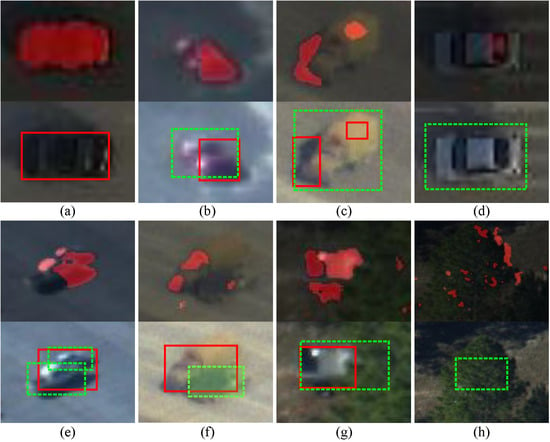
4.1.3. Detection Refinement

Figure 3 illustrates some inaccurate detections caused by two or more spatially close objects, which might increase the object’s identity switch and false alarms. Therefore, we proposed a detection refinement process to solve these problems. For the unmatched detection ${\mathbf{d}}_t^j\in {\mathbb{D}}_t^{U_1}$ after Stage 1, we deleted inaccurate detections from ${\mathbb{D}}_t^{U_1}$ when their bounding box overlapped with more than two unmatched objects updated by the FCT appearance-based prediction. Thus, the inaccurate detections in Figure 3b,c,e–g would be deleted if they were not associated with any tracklets. After this detection refinement step, all remaining unmatched detections ${\mathbf{d}}_t^j\in {\mathbb{D}}_t^{U_1}$ are used in Stage 2, along with the unreliable tracklets in ${\mathbb{T}}_t^{A\left(l\right)}$.

4.2. Stage 2: Handling Drifting Tracklets

In complex airborne videos situations, where objects are occluded as the mounted camera changes its motion, conventional online tracking methods, based on a simplified motion model (e.g., the used KF-based constant velocity model), are prone to producing drifting problems [27,44]. If the object continues drifting, it is difficult to re-assign the object to detections or re-appearing objects (Occlusion-I and Occlusion-II). In the proposed framework, the second association stage solves the reassignment problem between unreliable tracklets ${\mathbb{T}}_t^{A\left(l\right)}$ and unmatched detections ${\mathbb{D}}_t^{U_1}$ not associated during the first stage. An unreliable tracklet in ${\mathbb{T}}_t^{A\left(l\right)}$ is converted into a reliable tracklet in ${\mathbb{T}}_t^{A\left(h\right)}$ if it can be re-associated with a detection; otherwise, it maintains the same state or is converted to an inactive tracklet in ${\mathbb{T}}_t^{I_o\left(l\right)}$ after the state update.

Two aspects are considered in this stage: (1) If the object is occluded by an occluder, it might re-appear again around the occluder. The unmatched detection near the occluder has a high possibility of being re-associated with the re-appearing object after occlusion. (2) If the object has been occluded by environmental obstacles, it might re-appear at any position in the image. We assumed that the occluded object might re-appear in a limited region around the occluder. The longer the object disappears, the larger the required search region.

4.2.1. Second Association via the Affinity Score

For the current frame t, the input pairs of this association stage are $\{(T_t^i,{\mathbf{d}}_t^j)|\forall T_t^i\in {\mathbb{T}}_t^{A\left(l\right)},\forall {\mathbf{d}}_t^j\in {\mathbb{D}}_t^{U_1}\}$. The affinity of the second association is defined as:

$${\mathsf{\Lambda }}^2\left(T_t^i,{\mathbf{d}}_t^j\right)=\left\{\begin{array}{cc}{\mathsf{\Lambda }}_a^1(T_t^i,{\mathbf{d}}_t^j)\exp \left(\mathsf{\Omega }\left(T_t^k\right)\right),& \mathrm{if}{\zeta }_s^2\left(T_t^i\right)=T_t^k,dist({\mathbf{d}}_t^j,T_t^k)\le {\Delta }_t^{i\left(l\right)}\\ {\mathsf{\Lambda }}_a^1(T_t^i,d_t^j),& \mathrm{if}{\zeta }_s^2\left(T_t^i\right)=\varnothing ,dist({\mathbf{d}}_t^j,T_t^i)\le {\Delta }_t^{i\left(h\right)}\\ 0,& \mathrm{otherwise}\end{array}\right.$$

(25)

where ${\zeta }_s^2\left(T_t^i\right)$ is an operator that returns a possible occluder tracklet $T_t^k$ or ∅ to indicate that the occluder is an environmental obstacle. A tracklet $T_t^k$ is defined as an occluder of $T_t^i$ if the overlap ratio ${\zeta }_p({\mathbf{c}}_t^i,T_t^k)$, defined in Equation (23), between the bounding box of the FCT-based tracker ${\mathbf{c}}_t^i$ of $T_t^i$ and the bounding box of the tracklet $T_t^k$ is less than a given overlapping threshold $t{h}_o$, i.e., ${\zeta }_p({\mathbf{c}}_t^i,T_t^k)\ge t{h}_o$. The function $dist({\mathbf{d}}_t^j,T_t^k)$ is the Euclidean distance between the location of a detection ${\mathbf{d}}_t^j$ and the tracklet $T_t^k$. ${\Delta }_t^{i\left(l\right)}=\sqrt{(\frac{w_t^i+w_t^k}{2}{)}^2+(\frac{h_t^i+h_t^k}{2}{)}^2}$ is the maximum allowed distance for an acceptable detection near the occluder tracklet, $T_t^k$ to be associated with $T_t^i$, with $(w_t^i,h_t^i)$ and $(w_t^k,h_t^k)$ the width and height of the bounding box of tracklets $T_t^i$ and $T_t^k$, respectively. ${\Delta }_t^{i\left(h\right)}=\sqrt{{\left(w_t^i\right)}^2+{\left(h_t^i\right)}^2}{L}_M(1-\mathsf{\Omega }\left(T_t^i\right))$ is the maximum allowed distance of an acceptable detection to be associated with $T_t^i$, where $\mathsf{\Omega }(·)$ is the tracklet confidence and $L_M$ is the number of frames in which the i-th object is missing due to occlusion or unreliable detection, as defined in Equation (11).

4.2.2. Tracklet Correction

The second association allowed us to re-assign drifting tracklets to the detections of re-appearing objects in a limited time. An association score matrix $S^2$, the same as in Equation (19), is used to express the affinity score between the detections and the tracklets, and the Hungarian algorithm [41] is used to determine the tracklet-detection pairs with the lowest affinity value in $S^2$. After association, the state and the confidence values of the associated tracklets are updated with the associated detections using Equations (11) and (20), respectively. Here, to update the state of the re-appeared tracklet, we used only the matched detection and set $w_f=1$ in Equation (20). Finally, the trajectory within the drifting interval is corrected via linear interpolation between the previous and updated location of the tracklet.

4.3. Stage 3: New Active Tracklet Generation

The third association stage solves the assignment problem between the candidate tracklets ${\mathbb{T}}_{t-1}^C$ from the previous frame and the remaining unmatched detections ${\mathbb{D}}_t^{U_2}$ to generate new active tracklets ${\mathbb{T}}_t^{A_n\left(h\right)}$. The input pairs of this association in the current frame t are $\{(T_{t-1}^i,{\mathbf{d}}_t^j)|\forall T_{t-1}^i\in {\mathbb{T}}_{t-1}^C,\forall {\mathbf{d}}_t^j\in {\mathbb{D}}_t^{U_2}\}$. The affinity ${\mathsf{\Lambda }}^3(T_{t-1}^i,{\mathbf{d}}_t^j)$ and the association score matrix $S^3$ are the same as those used in Stage 1. When the candidate tracklet is associated in $t{h}_I$ consecutive frames ($t{h}_I$ = 5 frames in our experiments), it is converted into a new tracklet, for which we initialized an FCT appearance-based tracker. The matched to detection candidate tracklets are maintained in the candidate tracklet set ${\mathbb{T}}_t^C$ if the tracklet length is less than $t{h}_I$. The unmatched candidate tracklets, which are considered false-alarms, are removed from the candidate tracklet set.

4.4. Stage 4: Globally Linking Fragmented Tracklets

In challenging situations where the objects are constantly occluded by other objects or obstacles for a long time, tracklet fragmentation is likely to occur, and the same object can be divided into two or more tracklets, as illustrated in Figure 5. Motivated by the works in object re-identification [38,39] to build long-term object trajectories based on appearance modeling and matching, the fourth association stage of the proposed framework solves the assignment problem between the lost tracklets ${\mathbb{T}}_t^{I_o\left(l\right)}$ and the new tracklets ${\mathbb{T}}_t^{A_n\left(h\right)}$, linking these fragmented tracklets, re-identifying the lost objects and thereby building longer trajectories. As targets in airborne videos have similar appearances, false tracklet linking might occur if only based on the appearance modeling. Thus, both the appearance and motion terms are considered in the fourth stage.

4.4.1. Fourth Association via the Affinity Score

The input pairs of the forth association in the current frame t are the set $\{(T_t^i,T_t^j)|\forall T_t^i\in {\mathbb{T}}_t^{I_o\left(l\right)},\forall T_t^j\in {\mathbb{T}}_t^{A_n\left(h\right)}\}$. The affinity of the fourth association is defined as:

$${\mathsf{\Lambda }}^4\left(T_t^i,T_t^j\right)={\mathsf{\Lambda }}_a^4\left(T_t^i,T_t^j\right){\mathsf{\Lambda }}_m^4\left(T^i,T^j\right)$$

(26)

where ${\mathsf{\Lambda }}_a^4\left(T_t^i,T_t^j\right)$ and ${\mathsf{\Lambda }}_m^4\left(T_t^i,T_t^j\right)$ are the appearance and motion affinity score, respectively.

The appearance affinity ${\mathsf{\Lambda }}_a^4\left(T_t^i,T_t^j\right)$ is defined as:

$${\mathsf{\Lambda }}_a^4\left(T_t^i,T_t^j\right)=\max \left\{\frac{1}{N_H^i}\sum _{l\in [1,N_H^i]}\varsigma ({\chi }_{T^i}^l,T_t^j),\frac{1}{N_H^j}\sum _{m\in [1,N_H^j]}\varsigma ({\chi }_{T^j}^m,T_t^i)\right\}$$

(27)

where $N_H^i$ and $N_H^j$ are the number of templates of the tracklet $T_t^i$ and $T_t^j$, respectively; ${\chi }_{T^i}^l$ is the l-th template of tracklet $T_t^i$; ${\chi }_{T^j}^m$ is the m-th template of tracklet $T_t^j$; and $\varsigma ({\chi }_{T^i}^a,T_t^b)=\frac{1}{N_H^b}{\displaystyle \sum _{b\in [1,N_H^b]}}\rho ({\chi }_{T^i}^a,{\chi }_{T^j}^b)$, for $(a,b)=(l,j)$ and $(a,b)=(m,i)$. The motion affinity ${\mathsf{\Lambda }}_m^4\left(T_t^i,T_t^j\right)$ is evaluated between the tail of the history of the tracklet $T_t^i$ and the head of the tracklet $T_t^j$ with the time gap ${\mathsf{\Theta }}_t$ [11] based on a linear motion assumption:

$${\mathsf{\Lambda }}_m^4\left(T^i,T^j\right)=\mathcal{N}\left({\tilde{\mathbf{p}}}_i;{\mathbf{p}}_j^{head},m^F\right)\mathcal{N}\left({\tilde{\mathbf{p}}}_j;{\mathbf{p}}_i^{tail},m^B\right)$$

(28)

where ${\tilde{\mathbf{p}}}_i={\mathbf{p}}_i^{tail}+{\mathbf{v}}_i^F{\mathsf{\Theta }}_t$ and ${\tilde{\mathbf{p}}}_j={\mathbf{p}}_j^{head}+{\mathbf{v}}_j^B{\mathsf{\Theta }}_t$, ${\mathbf{p}}_i^{tail}$ and ${\mathbf{p}}_j^{head}$ represent the position of $T_t^i$ and $T_t^j$, ${\mathbf{v}}_i^F$ is the forward velocity of $T_t^i$ and ${\mathbf{v}}_j^B$ is the backward velocity of $T_t^j$ estimated using the KF with the latest and first $N_v^B$ states of the tracklet $T_t^i$ and $T_t^j$, respectively. $\mathcal{N}(·)$ is a Gaussian distribution function.

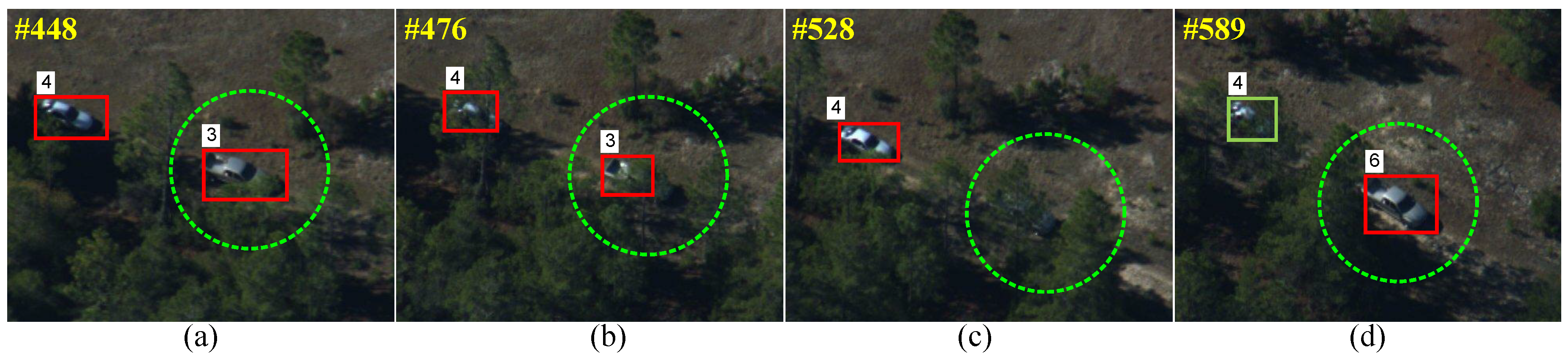
4.4.2. Object Re-Identification via Tracklet Linking

The association score matrix $S^4={\left[s_{ij}\right]}_{n_i^4\times n_j^4}$ with $s_{ij}=-\ln \left({\mathsf{\Lambda }}^4(T_t^i,T_t^j)\right)$ is used to express the affinity score between tracklets in the fourth stage. The Hungarian algorithm [41] is used to determine the $(i,j)$ pairs of tracklets with the maximum affinity in $S^4$. The tracklet $T_t^j$ is associated with $T_t^i$ when the association cost $s_{ij}$ is less than a pre-defined threshold $\theta$ [11]. If a lost tracklet $T_t^i$ and a new tracklet $T_t^j$ are associated, they are considered as the same object and merged, and their trajectories are linked with a linear interpolation. We assigned the ID of the lost tracklet $T_t^i$ to the new tracklet $T_t^j$. Thus, the lost objects are re-identified using the above tracklet linking process.

The remaining inactive tracklets that have not been reassigned to new tracklets are either terminated if $t-t_e^i\ge t{h}_e$ ($t{h}_e$ = 40 frames in our experiments) or kept in the inactive tracklets set ${\mathbb{T}}_t^{I_o\left(l\right)}$.

5. Experiments

The proposed hierarchical association framework for multiple object tracking in airborne video is implemented in MATLAB on a desktop PC with an Intel Core 2.40 GHz CPU with 32 GB RAM. In the following, we evaluate its performance considering several airborne video sequences.

5.1. Datasets

We evaluated our approach on two datasets, the Video Verification of Identity (VIVID) dataset [45] and the Shaanxi provincial key laboratory of speech and Image Information Processing (SAIIP) dataset. Figure 6 illustrates some images from the datasets. The VIVID dataset includes five visible data sequences and three thermal Infrared (IR) data sequences. The VIVID datasets have been collected over the Eglin Air Base and the Fort Pickett base under the framework of the DARPA VIVID program [45]. The SAIIP dataset includes four sequences that were captured over a provincial road using the DJI PHANTOM-3-4K quad-copter.

Table 1. Used benchmark sequences: Illumination Variation (IV), Scale Variation (SV), Occlusion (OCC), Background Occlusion (BOC), Motion Variation (MV), Image Blurring (IB), and Shadow Interference (SI).

Dataset	Sequence	Image Size	# of Frames	# of Targets	IV	SV	OCC	BOC	MV	IB	SI
VIVID	EgTest01	680 × 480	1821	6	√	√	×	×	√	×	√
	EgTest02	680 × 480	1302	6	√	√	√	×	√	×	√
	EgTest03	680 × 480	2571	6	√	√	√	×	√	×	√
	EgTest04	680 × 480	1833	5	√	×	×	√	√	√	√
	EgTest05	680 × 480	1764	4	√	√	×	√	√	×	√
	PkTest01	680 × 480	1460	5	√	√	√	√	×	×	×
	PkTest02	680 × 480	1595	12	√	√	×	√	√	×	×
	PkTest03	680 × 480	2011	7	√	×	×	√	√	×	×
SAIIP	SpTest01	1920 × 1080	1763	37	√	×	×	×	×	×	×
	SpTest02	1920 × 1080	1689	42	√	√	×	×	√	×	×
	SpTest03	1920 × 1080	1624	29	√	√	×	×	√	×	√
	SpTest04	1920 × 1080	1206	46	√	√	×	√	√	×	√

lists the different sequences, their number of frames, the number of targets involved, as well as their main challenges, including Illumination Variation (IV), Scale Variation (SV), Occlusion (OCC), Background Occlusion (BOC), Motion Variation (MV), Image Blurring (IB) and Shadow Interference (SI).

In the EgTest01 sequence, the vehicles loop around a runway and then drive straight. Some vehicles are similar in appearance. In the EgTest02 sequence, two sets of three vehicles pass each other on a runway. Changes of scaling occur because the airborne camera circles the scene. The data association for the EgTest02 sequence is more difficult than for the EgTest01 sequence due to severe occlusions. This also occurs in the EgTest03 sequence, where two sets of three vehicles pass each other on a runway. In the EgTest04 sequence, a line of vehicles travels down a red dirt road. In the EgTest05 sequence, a vehicle moves along a dirt road in a wooded area. Occlusion and illumination variations occur when the vehicle passes in and out of tree shadows.

The sequences of PkTest01, PkTest02 and PkTest03 are thermal IR data. In the PkTest01 sequence, the vehicles are frequently occluded by the trees. In the PkTest02 sequence, the vehicles stop at an intersection, then continue. The main issues include occlusion, shadows and camera auto-gain. The thermal IR contains a line of vehicles in a stop-and-go scenario in the PkTest03 sequence. As in the previous sequence, occlusions, shadows and camera auto-gain are prevalent in this sequence. Moreover, the vehicles are small, and the camera viewpoint is nearly nadir.

All the sequences from the SAIIP dataset (SpTest01, SpTest02, SpTest03 and SpTest04) were captured over a provincial road. There are fewer occlusions because the camera is pointed at the road to take the videos, and most of the vehicles are moving at a high speed while maintaining a safe distance from each other. However, several targets have a similar appearance, and some stop at the crossroad. There are also some trucks with a long body, which might be detected as two separate objects.

5.2. Parameter Setting

In the following, we describe the parameter setting of each module of the framework.

5.2.1. Detector Parameters

We first compared three motion compensation-based detectors and then analyzed the parameters setting of the used detector. The three compensation-based detectors included the Basic Compensation-based Detector (BCD) [20], the MHI detector [20] and the SGM detector [23]. All source codes were provided by the authors. For a fair comparison, the same parameter settings used by the authors in their original publication were used. Both BCD and MHI detectors assume a pre-defined threshold ($T_{\theta }$ = 20) to determine the detections in each image. The SGM detector relies on a grid size of $T_{\theta }\times T_{\theta }$ with $T_{\theta }$ = 10 [23] for determining the detections.

For the quantitative evaluation of detector performance, we used the Detection Ratio (DTR) $r_D=N_O^D/N_O^T$ and the False-Alarm Ratio (FAR) $r_F=(N_O^A-N_O^T)/N_O^A$, where $N_O^D$ represents the effective number of detected objects, $N_O^T$ represents the number of true objects and $N_O^A$ represents the total number of detections. A detection with bounding box $B_D$ is considered successful if $SR=\frac{Area(B_D\cap B_{GT})}{Area(B_D\cup B_{GT})}\ge T_{SR}$ (in our experiments $T_{SR}=0.5$) for a ground truth bounding box $B_{GT}$. To analyze the influence of the threshold $T_{\theta }$ on the considered motion compensation-based detectors appropriately, we defined different values of $T_{\theta }^v=10\times {\theta }_v$, with ${\theta }_v=\{0.5,0.75,1,1.25,1.5\}$. As shown in Figure 7, the MHI-based approach can efficiently reduce FAR compared with the BCD- and SGM-based approaches. However, the required forward motion history is not suitable for practical applications. In our implementation, we selected the SGM-based detector, which has comparable DTR and FAR to the MHI-based approach, while performing in real time.

The detection performance depends on the velocity of the tracked objects and the complexity of the background when using motion-based compensation approaches. As such, a single fixed determining threshold $T_{\theta }$ was not suitable for all test sequences.

Table 2. Comparison of detection results with different detection thresholds $T_{\theta }^v$. DTR, Detection Ratio; FAR, False-Alarm Ratio.

Threshold	VIVID			SAIIP
	DTR%	FAR%	FPS	DTR%	FAR%	FPS
$T_{\theta }^1$	91.7	36.7	18	97.3	12.8	9
$T_{\theta }^2$	85.6	28.4	22	94.4	10.3	12
$T_{\theta }^3$	81.3	18.6	28	91.7	8.7	16
$T_{\theta }^4$	72.9	14.2	32	88.5	6.6	20
$T_{\theta }^5$	68.4	10.5	37	86.9	5.9	27

lists the DTR and FAR, along with the computational cost in terms of Frames Per Second (FPS), of the SGM-based detector with different determining thresholds on the VIVID dataset and SAIIP dataset. Notably, on the VIVID dataset, both the DTR and FAR ratios decreased with increasing values of the determining threshold. The obtained results on the SAIIP dataset were similar, but less computation was required when the determining threshold was increased. The computation cost on the SAIIP dataset was higher than on the VIVID dataset due to the larger image size.

For the experiments reported in the following sections, we set $w^d=0.5$ in Equation (11) and $T_{\theta }=10$ for the five visible data sequences and $T_{\theta }=5$ for the three thermal IR data sequences of the VIVID dataset. For the SAIIP dataset, we set $T_{\theta }=15$ and $w^d=0.7$. Note that $w^d$ is set to a large value when the detector is highly accurate [11].

5.2.2. Hierarchical Framework Parameters

All parameters of the tracking framework have been set empirically and remained unchanged for all datasets.

• For the affinity models of Equations (15) and (26), the parameters $m^F$ and $m^B$ were set to diag $\left[{30}^2{75}^2\right]$.
• The same threshold $\theta =0.4$ was used for the association score matrices $S^1$, $S^2$, $S^3$ and $S^4$ to determine the association results.
• For the FCT trackers in our experiments, the search radius for drawing positive samples in the online appearance-based classifier was set to $\alpha$ = 4 to generate 45 positive samples. The inner and outer radii for the negative samples were set to $\beta =8$ and $\zeta =30$, respectively, to randomly select 50 negative samples. The initial learning rate $\lambda$ of the classifier was set to 0.9. The size of the random matrix was set to 100.
• For the Kalman filter model, the process (Q) and measurement (R) noise covariance matrices were set as $Q=\left[\begin{array}{cccc}0.0025& 0& 0.0025& 0\\ 0& 0.0025& 0& 0.0025\\ 0.0025& 0& 0.0025& 0\\ 0& 0.0025& 0& 0.0025\end{array}\right]$, and $R=\left[\begin{array}{cc}0.1& 0\\ 0& 0.1\end{array}\right]$, respectively.

5.3. Comparison with State-of-the-Art Frameworks

To demonstrate the tracking performance of our proposed framework, we compared it to the MOT approaches of [11] and [14] on the selected datasets. All the approaches, including ours, adopt the same detection configuration, and a window size of five frames was defined to remove unreliable shorter tracklets. For both [11] and [14], we used publicly available codes provided by the authors.

5.3.1. Evaluation Metrics

The popular evaluation metrics as defined in [46] were used for performance evaluation. Denoting by GT the number of trajectories in the Ground-Truth, we estimate the Mostly Tracked targets (MT), the Mostly Lost targets (ML) and the Partially Tracked (PT) objects. Furthermore, the Precision (PR), defined as the correctly-matched objects over the total output objects, and the total number of Identity Switches (IDS) are used. They are summarized in

Table 3. Evaluation metrics [46]. PR, Precision.

Name	Definition
PR	Correctly-matched objects/total output objects (frame-based);
GT	Number of Ground-Truth trajectories.
MT	Mostly Tracked: percentage of GT trajectories that are covered by the tracker’s output for more than 80% in length.
ML	Mostly Lost: percentage of GT trajectories that are covered by the tracker’s output for less than 20% in length. The smaller the better.
PT	Partially Tracked: 1.0-MT-ML.
IDS	ID Switches: the total of number of times that a tracked trajectory changes its matched GT identity. The smaller the better.

.

5.3.2. Comparison of Data Association

A qualitative comparison between different versions of the proposed system on sequence EgTest02 is provided in

Table 4. Comparison of tracking results on sequence EgTest02 with different detection thresholds $T_{\theta }^v$ (${\theta }_1=0.5$, ${\theta }_3=1$, ${\theta }_5=1.5$). Best results are underlined.

Method	MT (%)			ML (%)			IDS
	${\mathit{T}}_{\mathit{\theta }}^1$	${\mathit{T}}_{\mathit{\theta }}^3$	${\mathit{T}}_{\mathit{\theta }}^5$	${\mathit{T}}_{\mathit{\theta }}^1$	${\mathit{T}}_{\mathit{\theta }}^3$	${\mathit{T}}_{\mathit{\theta }}^5$	${\mathit{T}}_{\mathit{\theta }}^1$	${\mathit{T}}_{\mathit{\theta }}^3$	${\mathit{T}}_{\mathit{\theta }}^5$
${\mathbf{S}}_1$	86.6	80.6	76.3	3.8	8.6	16.4	24	20	27
${\mathbf{S}}_2$	92.1	86.1	80.5	2.1	6.8	10.7	12	9	13

. Two versions were considered:

• S${}_1$ corresponds to the framework without tracklets analysis and detection refinement. The method presented by [11] was used to estimate the tracklet state. The position and the velocity of the matched tracklets were updated with the associated detection, whereas the unmatched tracklets were updated using the KF motion-based predictions. The size of the object was updated by averaging the associated detection of the recent past frames.
• S${}_2$ is the fully-proposed framework as illustrated in Figure 1, denoted as HATAin the following.

Comparing the results of frameworks S${}_1$ and S${}_2$, the effect of the tracklet analysis and detection refinement processes in the proposed framework S${}_2$ is noticeable. Notice from Table 4 that the system S${}_1$ performs well for the MT and ML measures. The high false alarm rate and unreliable detections cause a high IDS measure, due to the inaccurate location and size of the detections, which affects the association between tracklets and detections. As expected, the proposed framework S${}_2$ performed better for most metrics, efficiently reducing the IDS measure compared to S${}_1$. Figure 8 illustrates the tracking results of S${}_1$ and S${}_2$ using the threshold $T_{\theta }^3$ on sequence EgTest02. As shown in Figure 8, the ID-2 and ID-3 targets in Frame #390 have an accurate location and size using the framework S${}_2$, even with inaccurate detection inputs. This is due to the use of the FCT tracker to correct the state of the tracklet, as obtained with Equation (20). Similarly, S${}_2$ performs well in Frame #460 with the help of the tracklet analysis and detection refinement process, which efficiently avoided the false new tracklet generation (ID-11 in system S${}_1$). This also occurs in Frame #532.

5.3.3. Comparisons to Other MOT Frameworks

A quantitative comparison between our proposed framework and state-of-the-art algorithms is outlined in

Table 5. Tracking results on the selected datasets. The best results are underlined.

Sequence	GT	Method	PR (%)	MT (%)	ML (%)	PT (%)	IDS
EgTest01		Bae et al. [11]	90.7	94.4	3.6	2.0	2
	6	Prokaj et al. [14]	88.6	93.6	3.2	3.2	4
		Proposed HATA	94.8	96.8	2.9	0.3	2
EgTest02		Bae et al. [11]	78.8	80.6	8.6	11.8	28
	6	Prokaj et al. [14]	70.5	69.3	5.4	25.3	41
		Proposed HATA	84.4	86.1	6.8	7.1	13
EgTest03		Bae et al. [11]	82.6	80.7	6.8	12.5	20
	6	Prokaj et al. [14]	77.8	74.3	5.4	20.3	29
		Proposed HATA	87.1	83.6	4.7	11.7	11
EgTest04		Bae et al. [11]	82.9	78.9	4.9	16.2	19
	5	Prokaj et al. [14]	76.4	73.2	6.6	20.2	28
		Proposed HATA	85.3	81.8	5.6	12.6	12
EgTest05		Bae et al. [11]	68.9	75.2	6.7	18.1	42
	4	Prokaj et al. [14]	70.8	81.2	5.3	13.5	60
		Proposed HATA	78.6	86.4	5.7	7.9	23
PkTest01		Bae et al. [11]	79.6	82.3	5.3	12.4	20
	5	Prokaj et al. [14]	74.3	78.7	10.2	11.1	36
		Proposed HATA	88.8	89.1	2.1	8.8	14
PkTest02		Bae et al. [11]	76.9	73.8	5.9	20.3	23
	12	Prokaj et al. [14]	72.9	69.7	7.2	23.1	38
		Proposed HATA	83.4	79.4	5.1	15.5	15
PkTest03		Bae et al. [11]	72.9	78.6	6.4	15.0	29
	7	Prokaj et al. [14]	68.4	74.5	8.2	17.3	42
		Proposed HATA	79.1	81.9	5.8	12.3	16
SpTest01		Bae et al. [11]	97.6	94.7	0.9	5.4	5
	37	Prokaj et al. [14]	93.3	92.6	2.8	7.6	9
		Proposed HATA	98.5	96.4	0.5	3.1	2
SpTest02		Bae et al. [11]	88.9	83.8	9.8	6.4	18
	42	Prokaj et al. [14]	82.9	77.9	12.2	9.9	22
		Proposed HATA	93.5	91.4	6.2	3.4	7
SpTest03		Bae et al. [11]	87.2	85.6	10.8	3.6	17
	29	Prokaj et al. [14]	84.6	82.6	13.5	3.9	29
		Proposed HATA	89.8	91.2	6.9	1.9	11
SpTest04		Bae et al. [11]	89.3	87.9	8.4	3.7	26
	46	Prokaj et al. [14]	81.6	81.3	13.6	5.1	31
		Proposed HATA	91.7	93.4	4.1	2.5	12

. Both [11,14] achieved good results with the available detections, but performed poorly in terms of inaccurate detection. Instead, our algorithm was better with the chosen evaluation metrics (ML, MT and IDS). The qualitative tracking results of our approach are shown in Figure 9 and Figure 10.

Results using the VIVID dataset: Figure 9 illustrates the tracking results using the eight sequences from the VIVID dataset. For the EgTest01 sequence, all considered approaches performed well due to the reliable detections. Our proposed framework achieved the best results when the appearance and motion of the vehicles varied during the loop around period (Frames $\#28$, $\#172$ and $\#323$). In the EgTest02 sequence, two sets of vehicles pass each other on a runway and one set is occluded by the other set between Frames $\#443$, $\#482$ and $\#670$. Both [11,14] produce ID switches with most of the tracked targets, whereas HATA appropriately identified most of the tracklets. HATA also performed well in the EgTest03 sequence. In the EgTest04 sequence, only HATA solved the ID switching problem when the ID-3 vehicle was occluded by the trees in Frame $\#721$. In the EgTest05 sequence, HATA managed the occlusion in Frames $\#590$ and $\#701$ and the illumination changes when the targets passed in and out of the shadowed wooded area well.

Figure 9f,g illustrates the tracking results using the thermal IR sequences PkTest01, PkTest02 and PkTest03. In the PkTest01 sequence, only HATA accurately identified the vehicle that was frequently occluded by the trees between Frames $\#128$ and $\#278$. Our algorithm constantly tracked the vehicles that stopped at the intersection in Frame $\#561$ and resumed moving after Frame $\#654$ in the PkTest02 sequence. As with visible data, HATA solves the occlusion and illumination variation problems in IR data, as shown in Frames $\#833$ and $\#1229$. In the PkTest03 sequence, the vehicles are frequently occluded by trees after Frame $\#298$, and HATA robustly saved the correct ID for each tracked target in Frame $\#374$ and Frame $\#386$.

Results using the SAIIP dataset: Figure 10 illustrates the tracking results using the SAIIP dataset. For the SpTest01 sequence, all the moving objects were well detected (Figure 10a). HATA efficiently tracked all the detected objects. The false alarms were removed when the bounding box size was smaller than a pre-defined threshold $T_{fal}=5\times 5$. This strategy was also adopted for the sequences SpTest02, SpTest03 and SpTest04. The SpTest02 sequence was more challenging than the SpTest01 sequence as the vehicles slow their motion. HATA solves the motionless problem, as shown in Frames #564 and #709 of Figure 10b. Both the SpTest03 sequence and SpTest04 sequence were captured around a crossroad where the vehicles slow down, stop or change directions. In the SpTest03 sequence, as shown in Figure 10c, HATA accurately identified the ID-4 object when it changed direction in Frame #122. Moreover, HATA achieved long-term tracking for the ID-1 object in Frame #245. In the SpTest04 sequence, many vehicles pass through the crossroad. As shown in Figure 10d, HATA identified the ID-3 and ID-7 objects in Frame #98 and the objects with ID-3 and ID-10 in Frame #119.

The proposed method was implemented using MATLAB on a PC with an Intel Core 2.40-GHz CPU with 32 GB RAM without parallel and GPU processing. The average speed of the proposed method using the VIVID dataset was about 16 FPS and 13 FPS for the SAIIP dataset, excluding the detection step. The results show the improved performance of the proposed method compared to state-of-the-art methods. Compared to the framework proposed by Prokaj et al. [11], apart from including the online single-target tracking and object re-identification, our method integrates extra steps such as the tracklet analysis and detection refinement processes. This allowed solving drifting problems and tracklet fragmentation. The detection refinement process helped avoiding the generation of false new tracklets caused by unreliable detections.

6. Conclusions

In this paper, an online multi-object tracking method was proposed for airborne videos to solve the association problem caused by unreliable object detection. To robustly track objects in complex scenarios, we proposed an efficient hierarchical association framework based on the tracklet confidence and an FCT-based appearance tracking for multiple object tracking in airborne videos. The proposed framework appropriately handled tracklet generation, progressive trajectory construction and tracklet drifting and fragmentation. Each association stage of the hierarchical framework solved different assignment problems achieving reliable performance with 15 frames per second in MATLAB. The obtained results demonstrate the effectiveness of our framework compared to state-of-the-art methods. Improvements should be targeting three aspects: (1) a better object detector to reduce unreliable detections; (2) a better single-target tracking to deal with abrupt appearance change, which can cause unreliable matching; (3) a more sophisticated object re-identification in Stage 4. In the future, we will seek approaches that combine the proposed motion compensation-based detector with a deep online multi-object detection approach to reduce the false alarm rate of detections, as well as consider a deep learning approach for better object re-identification after long-term occlusion.

References

1. Wan, M.; Gu, G.; Qian, W.; Ren, K.; Chen, Q.; Zhang, H.; Maldague, X. Total Variation Regularization Term-Based Low-Rank and Sparse Matrix Representation Model for Infrared Moving Target Tracking. Remote Sens. 2018, 10, 510. [Google Scholar] [CrossRef]
2. Skoglar, P.; Orguner, U.; Törnqvist, D.; Gustafsson, F. Road Target Search and Tracking with Gimballed Vision Sensor on an Unmanned Aerial Vehicle. Remote Sens. 2012, 4, 2076–2111. [Google Scholar] [CrossRef] [Green Version]
3. Leitloff, J.; Rosenbaum, D.; Kurz, F.; Meynberg, O.; Reinartz, P. An Operational System for Estimating Road Traffic Information from Aerial Images. Remote Sens. 2014, 6, 11315–11341. [Google Scholar] [CrossRef] [Green Version]
4. Cao, Y.; Wang, G.; Yan, D.; Zhao, Z. Two Algorithms for the Detection and Tracking of Moving Vehicle Targets in Aerial Infrared Image Sequences. Remote Sens. 2016, 8, 28. [Google Scholar] [CrossRef]
5. Dey, S.; Reilly, V.; Saleemi, I.; Shah, M. Detection of independently moving objects in non-planar scenes via multi-frame monocular epipolar constraint. In Proceedings of the 12th European Conference on Computer Vision, Florence, Italy, 7–13 October 2012; pp. 860–873. [Google Scholar]
6. Yang, B.; Nevatia, R. Multi-target tracking by online learning of non-linear motion patterns and robust appearance models. In Proceedings of the 2012 IEEE Conference on Computer Vision and Pattern Recognition, Providence, RI, USA, 16–21 June 2012; pp. 1918–1925. [Google Scholar]
7. Luo, W.; Zhao, X.; Kim, T.K. Multiple object tracking: A review. arXiv, 2014; arXiv:1409.7618. [Google Scholar]
8. Reilly, V.; Idrees, H.; Shah, M. Detection and tracking of large number of targets in wide area surveillance. In Proceedings of the 11th European Conference on Computer Vision, Crete, Greece, 5–11 September 2010; pp. 186–199. [Google Scholar]
9. Berclaz, J.; Fleuret, F.; Turetken, E.; Fua, P. Multiple object tracking using k-shortest paths optimization. IEEE Trans. Pattern Anal. Mach. Intell. 2011, 33, 1806–1819. [Google Scholar] [CrossRef] [PubMed]
10. Pirsiavash, H.; Ramanan, D.; Fowlkes, C.C. Globally-optimal greedy algorithms for tracking a variable number of objects. In Proceedings of the 24th IEEE Conference on Computer Vision and Pattern Recognition, Colorado Springs, CO, USA, 20–25 June 2011; pp. 1201–1208. [Google Scholar]
11. Bae, S.H.; Yoon, K.J. Robust online multi-object tracking based on tracklet confidence and online discriminative appearance learning. In Proceedings of the IEEE Conference on Computer Vision and Pattern Recognition, Columbus, OH, USA, 23–28 June 2014; pp. 1218–1225. [Google Scholar]
12. Cheng, G.; Zhou, P.; Han, J. Learning Rotation-Invariant Convolutional Neural Networks for Object Detection in VHR Optical Remote Sensing Images. IEEE Trans. Geosci. Remote Sens. 2016, 54, 7405–7415. [Google Scholar] [CrossRef]
13. Li, K.; Cheng, G.; Bu, S.; You, X. Rotation-Insensitive and Context-Augmented Object Detection in Remote Sensing Images. IEEE Trans. Geosci. Remote Sens. 2017, 56, 2337–2348. [Google Scholar] [CrossRef]
14. Prokaj, J.; Duchaineau, M.; Medioni, G. Inferring tracklets for multi-object tracking. In Proceedings of the 2011 IEEE Computer Society Conference on Computer Vision and Pattern Recognition Workshops, Colorado Springs, CO, USA, 20–25 June 2011; pp. 37–44. [Google Scholar]
15. Xiao, J.; Cheng, H.; Sawhney, H.; Han, F. Vehicle detection and tracking in wide field-of-view aerial video. In Proceedings of the 2010 IEEE Computer Society Conference on Computer Vision and Pattern Recognition, San Francisco, CA, USA, 13–18 June 2010; pp. 679–684. [Google Scholar]
16. Prokaj, J.; Zhao, X.; Medioni, G. Tracking many vehicles in wide area aerial surveillance. In Proceedings of the 2012 IEEE Computer Society Conference on Computer Vision and Pattern Recognition Workshops, Providence, RI, USA, 16–21 June 2012; pp. 37–43. [Google Scholar]
17. Pollard, T.; Antone, M. Detecting and tracking all moving objects in wide-area aerial video. In Proceedings of the 2012 IEEE Computer Society Conference on Computer Vision and Pattern Recognition Workshops, Providence, RI, USA, 16–21 June 2012; pp. 15–22. [Google Scholar]
18. Prokaj, J.; Medioni, G. Persistent Tracking for Wide Area Aerial Surveillance. In Proceedings of the 2014 IEEE Conference on Computer Vision and Pattern Recognition, Columbus, OH, USA, 23–28 June 2014; pp. 1186–1193. [Google Scholar]
19. Yun, K.; Choi, J.Y. Robust and fast moving object detection in a non-stationary camera via foreground probability based sampling. In Proceedings of the 2015 IEEE International Conference on Image Processing, Quebec City, QC, Canada, 27–30 September 2015; pp. 4897–4901. [Google Scholar]
20. Yin, Z.; Collins, R. Moving object localization in thermal imagery by forward-backward MHI. In Proceedings of the Conference on Computer Vision and Pattern Recognition Workshop, New York, NY, USA, 17–22 June 2006; pp. 133–133. [Google Scholar]
21. Yu, Q.; Medioni, G. Motion pattern interpretation and detection for tracking moving vehicles in airborne video. In Proceedings of the 2009 IEEE Conference on Computer Vision and Pattern Recognition, Miami, FL, USA, 20–25 June 2009; pp. 2671–2678. [Google Scholar]
22. Kim, S.W.; Yun, K.; Yi, K.M.; Kim, S.J.; Choi, J.Y. Detection of moving objects with a moving camera using non-panoramic background model. Mach. Vis. Appl. 2013, 24, 1015–1028. [Google Scholar] [CrossRef]
23. Moo Yi, K.; Yun, K.; Wan Kim, S.; Jin Chang, H.; Young Choi, J. Detection of moving objects with non- stationary cameras in 5.8 ms: Bringing motion detection to your mobile device. In Proceedings of the IEEE Conference on Computer Vision and Pattern Recognition Workshops, Portland, OR, USA, 23–28 June 2013; pp. 27–34. [Google Scholar]
24. Bae, S.H.; Yoon, K.J. Robust Online Multiobject Tracking With Data Association and Track Management. IEEE Trans. Image Process. 2014, 23, 2820–2833. [Google Scholar] [PubMed]
25. Cao, X.; Wu, C.; Lan, J.; Yan, P. Vehicle Detection and Motion Analysis in Low-Altitude Airborne Video Under Urban Environment. IEEE Trans. Circ. Syst. Video Technol. 2011, 21, 1522–1533. [Google Scholar] [CrossRef]
26. Xing, J.; Ai, H.; Lao, S. Multi-object tracking through occlusions by local tracklets filtering and global tracklets association with detection responses. In Proceedings of the 2009 IEEE Conference on Computer Vision and Pattern Recognition, Miami, FL, USA, 20–25 June 2009; pp. 1200–1207. [Google Scholar]
27. Breitenstein, M.D.; Reichlin, F.; Leibe, B.; Koller-Meier, E.; Van Gool, L. Online multiperson tracking-by- detection from a single, uncalibrated camera. IEEE Trans. Pattern Anal. Mach. Intell. 2011, 33, 1820–1833. [Google Scholar] [CrossRef] [PubMed]
28. Ju, J.; Kim, D.; Ku, B.; Han, D.K.; Ko, H. Online Multi-object Tracking Based on Hierarchical Association Framework. In Proceedings of the IEEE Conference on Computer Vision and Pattern Recognition Workshops, Las Vegas, NV, USA, 26 June–1 July 2016; pp. 34–42. [Google Scholar]
29. Zhang, K.; Zhang, L.; Yang, M.H. Real-time compressive tracking. In Proceedings of the 12th European Conference on Computer Vision, Florence, Italy, 7–13 October 2012; pp. 864–877. [Google Scholar]
30. Zhang, K.; Zhang, L.; Yang, M.H. Fast compressive tracking. IEEE Trans. Pattern Anal. Mach. Intell. 2014, 36, 2002–2015. [Google Scholar] [CrossRef] [PubMed]
31. Ali, S.; Shah, M. COCOA: Tracking in aerial imagery. In Defense and Security Symposium; International Society for Optics and Photonics: Bellingham, WA, USA, 2006; p. 62090D. [Google Scholar]
32. Alatas, O.; Yan, P.; Shah, M. Spatio-temporal regularity flow (SPREF): Its Estimation and applications. IEEE Trans. Circ. Syst. Video Technol. 2007, 17, 584–589. [Google Scholar] [CrossRef]
33. Yalcin, H.; Hebert, M.; Collins, R.; Black, M.J. A flow-based approach to vehicle detection and background mosaicking in airborne video. In Proceedings of the 2005 IEEE Computer Society Conference on Computer Vision and Pattern Recognition, San Diego, CA, USA, 20–25 June 2005; p. 1202. [Google Scholar]
34. Cao, X.; Lan, J.; Yan, P.; Li, X. Vehicle detection and tracking in airborne videos by multi-motion layer analysis. Mach. Vis. Appl. 2012, 23, 921–935. [Google Scholar] [CrossRef]
35. Cao, X.; Gao, C.; Lan, J.; Yuan, Y.; Yan, P. Ego motion guided particle filter for vehicle tracking in airborne videos. Neurocomputing 2014, 124, 168–177. [Google Scholar] [CrossRef]
36. Cao, X.; Shi, Z.; Yan, P.; Li, X. Tracking vehicles as groups in airborne videos. Neurocomputing 2013, 99, 38–45. [Google Scholar] [CrossRef]
37. Liu, K.; Ma, B.; Zhang, W.; Huang, R. A spatio-temporal appearance representation for viceo-based pedestrian re-identification. In Proceedings of the IEEE International Conference on Computer Vision, Santiago, Chile, 7–13 December 2015; pp. 3810–3818. [Google Scholar]
38. Zapletal, D.; Herout, A. Vehicle Re-Identification for Automatic Video Traffic Surveillance. In Proceedings of the IEEE Conference on Computer Vision and Pattern Recognition Workshops, Las Vegas, NV, USA, 26 June–1 July 2016; pp. 25–31. [Google Scholar]
39. Liu, X.; Liu, W.; Ma, H.; Fu, H. Large-scale vehicle re-identification in urban surveillance videos. In Proceedings of the 2016 IEEE International Conference on Multimedia and Expo, Seattle, WA, USA, 11–15 July 2016; pp. 1–6. [Google Scholar]
40. Liu, X.; Liu, W.; Mei, T.; Ma, H. A Deep Learning-Based Approach to Progressive Vehicle Re-identification for Urban Surveillance. In Proceedings of the European Conference on Computer Vision, Amsterdam, The Netherlands, 8–16 October 2016; pp. 869–884. [Google Scholar]
41. Ahuja, R.K.; Magnanti, T.L.; Orlin, J.B. Network Flows: Theory, Algorithms, and Applications; Prentice Hall: Upper Saddle River, NJ, USA, 1993. [Google Scholar]
42. Kuo, C.H.; Huang, C.; Nevatia, R. Multi-target tracking by on-line learned discriminative appearance models. In Proceedings of the 2010 IEEE Computer Society Conference on Computer Vision and Pattern Recognition, San Francisco, CA, USA, 13–18 June 2010; pp. 685–692. [Google Scholar]
43. Qin, Z.; Shelton, C.R. Improving multi-target tracking via social grouping. In Proceedings of the 2012 IEEE Conference on Computer Vision and Pattern Recognition, Providence, RI, USA, 16–21 June 2012; pp. 1972–1978. [Google Scholar]
44. Yamaguchi, K.; Berg, A.C.; Ortiz, L.E.; Berg, T.L. Who are you with and Where are you going? In Proceedings of the 2011 IEEE Conference on Computer Vision and Pattern Recognition, Colorado Springs, CO, USA, 20–25 June 2011; pp. 1345–1352. [Google Scholar]
45. Collins, R.; Zhou, X.; Teh, S.K. An open source tracking testbed and evaluation web site. In Proceedings of the IEEE International Workshop on Performance Evaluation of Tracking and Surveillance, Breckenridge, CO, USA, 7 January 2005; pp. 17–24. [Google Scholar]
46. Li, Y.; Huang, C.; Nevatia, R. Learning to associate: Hybridboosted multi-target tracker for crowded scene. In Proceedings of the 2009 IEEE Conference on Computer Vision and Pattern Recognition, Miami, FL, USA, 20–25 June 2009; pp. 2953–2960. [Google Scholar]
Figure 1. The framework of the proposed algorithm. The symbols in the gray bounding box are the input to the processing stage, and the symbols in the white bounding box are the output.
Remotesensing 10 01347 g001
Figure 2. Tracklet status.
Remotesensing 10 01347 g002
Figure 3. Motion compensation-based detection. Red blobs correspond to detected moving objects. Red bounding-boxes are the detection results, and green dotted boxes are ground truth. (a) good detection. (b,c) partially detected object. (d) not detected object. (e) occluded object. (f) unreliable detection. (g) partially detected object. (h) occluded object.
Remotesensing 10 01347 g003
Figure 4. Illustration of Stage 1 association. The bounding boxes with the red color are the detection results. The bounding boxes with the green color are appearance-based predictions as a result of the Fast Compressive Tracker (FCT). The unmatched objects are marked with a yellow dotted circle and yellow color. (ad) Matched objects having a high tracklet confidence; (eh) matched objects having a low tracklet confidence.
Remotesensing 10 01347 g004
Figure 5. Fragmented tracklet under long-term occlusions. (a) Two tracked objects ID-3 and ID-4; (b) the object ID-3 is partially occluded and (c) heavily occluded by trees; (d) the lost object ID-3 is switched to ID-6 when it reappears again after the occlusion.
Remotesensing 10 01347 g005
Figure 6. Scenes from the public Video Verification of Identity (VIVID) dataset (first two rows) and the Shaanxi provincial key laboratory of speech and Image Information Processing (SAIIP) dataset (last row).
Remotesensing 10 01347 g006
Figure 7. Performance comparison of different motion compensation-based detectors. MHI, Motion History Images; BCD, Basic Compensation-based Detector; SGM, Single Gaussian Model.
Remotesensing 10 01347 g007
Figure 8. Detection and tracking results. First row: the detection results. Second row: the bounding box for each detection. Third row: the tracking results using the framework S 1 . Fourth row: the tracking results using the framework S 2 .
Remotesensing 10 01347 g008
Figure 9. The results on eight sequences from the VIVID dataset.
Remotesensing 10 01347 g009
Figure 10. The results on four sequences from the SAIIP dataset.
Remotesensing 10 01347 g010