Airborne and Terrestrial Laser Scanning Data for the Assessment of Standing and Lying Deadwood: Current Situation and New Perspectives


Department TESAF, University of Padova, viale dell’Università, 16, I-35020 Legnaro (PD), Italy
*
Author to whom correspondence should be addressed.
Remote Sens. 2018, 10(9), 1356; https://doi.org/10.3390/rs10091356
Submission received: 19 July 2018
/
Revised: 21 August 2018
/
Accepted: 24 August 2018
/
Published: 26 August 2018
(This article belongs to the Special Issue Innovative Remote Sensing for Monitoring and Assessment of Natural Resources)
Abstract
:LiDAR technology is finding uses in the forest sector, not only for surveys in producing forests but also as a tool to gain a deeper understanding of the importance of the three-dimensional component of forest environments. Developments of platforms and sensors in the last decades have highlighted the capacity of this technology to catch relevant details, even at finer scales. This drives its usage towards more ecological topics and applications for forest management. In recent years, nature protection policies have been focusing on deadwood as a key element for the health of forest ecosystems and wide-scale assessments are necessary for the planning process on a landscape scale. Initial studies showed promising results in the identification of bigger deadwood components (e.g., snags, logs, stumps), employing data not specifically collected for the purpose. Nevertheless, many efforts should still be made to transfer the available methodologies to an operational level. Newly available platforms (e.g., Mobile Laser Scanner) and sensors (e.g., Multispectral Laser Scanner) might provide new opportunities for this field of study in the near future.
1. Introduction
Deadwood in forest stands has often been considered a management problem in the past and its presence is still an issue, especially in producing forests, since it can be a possible source of pest outbreak, enhance fire risk, and represent a threat to worker/public safety [1]. On the other hand, deadwood is one of the most important indicators of habitat quality, hosting and providing nourishment to many of the most threatened forest species among insects [2], bryophytes, lichens [3], small mammals, and birds [4]. Furthermore, deadwood is important in microsite-enhancement for forest regeneration, particularly after high-severity disturbances [5]. For this reason, deadwood cover may be used as an indicator of microclimatic and micro-topographic habitat availability and heterogeneity [6]. Deadwood also plays a fundamental role in the carbon balance of forest ecosystems. Due to its increasing importance, National Forest Inventories (NFI) worldwide are now progressively including deadwood as a target component and its quantification is becoming of great interest [7,8,9,10,11,12,13]. Countries with a longer tradition of productive forestry are already assessing the impacts of biomass exploitation and strict production management [14,15,16,17], and their effect on deadwood presence.
Quantity is no longer considered the only valuable parameter for deadwood assessment, both for carbon sequestration [18,19] and biodiversity conservation purposes. For the latter, many authors highlight the importance of the size and decay stage of the deadwood component [20,21,22,23], even proposing specific taxa-based forest management [24,25].
This perspective is leading researchers to define new methodologies (e.g., [26,27]) for its identification and assessment of the amount and quality in different landscapes and throughout forest development stages [28,29,30]. In this direction, techniques from the field of remote sensing provide a valuable set of approaches for the study across wide scales. Among these, LiDAR is becoming an established technology for large-scale monitoring within the environmental sector [31], passing from direct applications in meteorology, topography, and forest planning. Within the latter, assessment of the aboveground biomass is no longer such a priority issue. There are many reported results from direct experiences of local administrations, academia, and funded projects (e.g., NEWFOR for EU) [32].
Ecological studies are increasingly using this technology, due to its capacity of collecting three-dimensional (3D) metrics of vegetation structure. As Davies and Asner [33] described in their review, most forest wildlife depends on all three dimensions of the environment. Using LiDAR-derived data on wildland structure, it is possible to better link species’ ecology to prediction mapping of occurrence or habitat suitability [34].
Although on the one hand it is true that mapping large areas has become quite easy and less expensive, on the other not all remotely sensed data are able to respond in the same way to small-scale events. As the general approach is progressively shifting from the global to the local scale, UAV (Unmanned Aerial Vehicle) technology has seen a rapid evolution within recent years and its easily affordable price has driven research to a further change in viewpoint. Rapid and complete remotely sensed monitoring can be conducted with UAVs, allowing for small-scale updates/adjustments of the original database. Indeed, their versatility allows point clouds to be obtained both from UAV-borne LiDAR sensors and from a ‘Structure from Motion’ procedure applied on photogrammetry surveys.
While LiDAR technology has become a reliable tool for forest structural parameter definition [35,36], the integration of different sources of remote sensing data (e.g., aerial imagery and LiDAR) is still an open frontier for forest ecologists [37].
This paper aims to give an overview on the current situation and future perspectives of this specific but heterogeneous topic. The first section introduces the definition and classification of deadwood in forest ecology and the importance of remote sensing LiDAR technology for its assessment. In the second, the specific applications of the two main remote sensing approaches (i.e., airborne and terrestrial) are discussed and compared. The third section reports on data-integration between the two approaches and data-fusion with other data sources. The fourth section describes multi-temporal applications for change detection and quantification. Examples of operational applications are provided to broaden the discussion within the perspective of environmental management. In the conclusions, critical points and future prospects are highlighted for the identification of knowledge gaps and research opportunities.
Deadwood
Coarse woody debris (CWD), as well as its properties and dynamics, were thoroughly described for the first time by Harmon et al. [38]. This wide category covers a variety of types and size of materials (Figure 1), including snags (or standing deadwood), logs, chunks of wood (as a result of the disintegration of the two previous types), large branches, stumps, and coarse roots. The same authors reported how size varied differently depending on the country and type of study, ranging from 2.5 to 7.5 cm as concerns the minimum diameter. Ten years later, Harmon and Sexton [39] defined the first specific guidelines for the U.S. forest inventories, setting 10 cm and 1 m as diameter and length thresholds to distinguish CWD from finer material called fine woody debris (FWD). An exception was proposed for forest fuels assessment, providing a minimum threshold of 7.5 cm [39].
The use of common thresholds by the scientific community has increased since their first proposal (see [38,39]), but differences can still be found in terms of both terminology and adopted thresholds. This lack of harmonization leads to a flaw in the comparison of different studies [40] or data sources. As an example, within the National Forest Inventories (NFI) of some European countries, the distinction between CWD and FWD is made according to a threshold of 10 cm in Scandinavian countries (Sweden, Norway, and Finland) and Italy, 7 cm in Switzerland and France, and 20 cm in Austria and Germany [11].
No ecological study has provided a clear threshold for distinguishing between fine and coarse woody debris [41], even though the choice of a specific definition can have a strong effect on deadwood quantification. Indeed, testing the exclusion of different deadwood elements from the total amount derived from the available NFI data, it is possible to see how adding just stumps can cause a 44% increase in volume [42].
Due to the diverse types of dead material that can be found within the forest environment, a literature search was conducted, identifying specific keywords (e.g., “LiDAR” AND “deadwood”, “LiDAR” AND “coarse woody debris”, etc.) in the main research platforms (e.g., Science Direct, Web of Science). Additional material was collected by searching through the bibliography available in each paper and including relevant grey literature. The selected papers were then screened to assess the real presence of the research topic, often present as a side-line of main methodologies developed for other purposes.
2. Airborne Laser Scanning
2.1. State of the Art: Data Types and Analysis
Within the last decade, due to technology developments and the increase in expertise, the LiDAR sector has been facing a progressive shift from different points of view:
- Data quality: improved accuracy in terms of data localization and measures
- Data density: from low- to high-density (e.g., single photon counting LiDAR)
- Data types: from discrete return to full waveform
- Analysis approach: from area-based to single-tree approaches
Analysis of the data may differ depending on the aggregation level at which the point cloud information is studied. The target information can be represented at a single-tree level [43] or according to a regular grid, where each cell summarizes the characteristics of the individuals included. The latter method is known as the area-based approach (ABA). The aggregation level is entangled with the point cloud quality due to the fact that low-density data can hardly be processed to obtain detailed information at a single-tree level. For this reason, the ABA was mostly used in early studies, when the available point densities were pretty low (i.e., <2 pts/m2). It leads to very good results, even if mostly for mapping purposes such as biomass estimation (e.g., [44,45,46,47,48,49]), information for forest fire management [50,51], and habitat modeling [52]. Even if high-density datasets are becoming more available, finer elaborations (i.e., single-tree) are still performed mainly for research purposes.
2.2. Area-Based Approach
The assessment of deadwood amount through the area-based approach is mainly indirectly derived from the living biomass parameters of forest stands. Ranius et al. [53] modelled the amount of deadwood from the growth of living trees, tree mortality rate, and CWD decomposition rate. They achieved accurate results only at the landscape level for Norway spruce stands without disturbances.
Common point cloud statistics extracted from low-density datasets have been used to estimate different components of deadwood such as standing and downed dead trees [54,55] or the potential logging residues following forest management operations [56]. The models, applied mostly to boreal/temperate conifer stands, resulted in accuracies ranging between 50% and 80%. Within a natural old-growth forest, canopy gaps have been classified according to the presence/absence of CWD using metrics extracted from the data between the ground and a height of 5 m [57].
The predictive power of ABA models mainly increases with stand maturity, but the accuracy of the models for predicting CWD volume using characteristics of living trees as predictors has been rather poor [41].
In a case study in the coastal forest of the U.S. Pacific Northwest [58], LiDAR-derived variables from a low-density dataset (<1 pts/m2) were compared to field data dividing deadwood in wildlife tree (WT) classes depending on its decay status. The coefficient of variation (log transformed) was found to be the best predictor variable within the modeling of the WT classes and, therefore, was the best predictor for the presence of deadwood. This result is consistent with those obtained by other authors (e.g., [59,60,61]) for the description of canopy structural attributes.
The Random Forest (RF) algorithm was adopted using LiDAR-derived metrics to predict total, live, dead, and percentage of dead basal area (BA) [62]. The investigation proved the significance of height and density metrics for predicting total BA, intensity, and density metrics for predicting living BA, and intensity metrics (mean, CV, and kurtosis) for predicting dead and percentage dead BA. Furthermore, in one plot the intensity normalization improved RF models predicting Dead and %Dead BA, demonstrating the importance of the use of intensity in distinguishing dead from live canopies.
Finally, Sumnall et al. [63] compared the use of Discrete Return (DR) and Full Waveform (FWF) data for modeling 23 different forest structure and composition parameters, including deadwood volume and decay stages for both standing and downed trees. Among the best-performing models, the standing deadwood volume obtained a prediction accuracy equal to an NRMSE of 16%. However, it was pointed out that the selection of LiDAR survey season (leaf-on/leaf-off) had greater importance than data type (i.e., DR or FWF) when determining the predictive power of the best-performing models.
2.3. Single-Tree Approach
2.3.1. Standing Deadwood
The identification of single standing dead trees (snags) using LiDAR data has only recently been addressed, due to the increase in high-quality and high-density data availability as well as segmentation methods required to work directly with the point cloud. Segmentation is the process aimed to delineate an object and its characteristics which, in forestry, means tree crowns, tree position, and dendrometric parameters (i.e., DBH, height), from remotely sensed data. The analysis approaches evolved from image segmentation techniques developed for aerial imagery and lately applied to 3D data (i.e., LiDAR).
It is possible to say that the paper by Reitberger et al. [64] was a forerunner in the field. In their study, indeed, some of the main approaches for canopy segmentation were tested with both DR and FWF LiDAR data. Not considering the difference in computation effort between the two data types, it is important to note that the “normalized cut segmentation” algorithm [65] was introduced into the analysis process. This technique has been successfully used through voxels applied on 3D point clouds in order to differentiate points belonging to each single tree. If compared to watershed segmentation that relies on a 52% detection rate, its application increases the detection rate to 60%, both considering the support given by the stem detection method [66]. An important aspect is the increase in detection of individuals in the lower and mid canopy layers, often rather difficult to identify due to clustering with the upper ones (e.g., [67]). Most studies were conducted on conifer stands where the size and shape of tree crowns are quite well defined. As described in Vauhkonen et al. [68], these assumptions allow site-/species-specific methods to be applied that cannot be easily used in different stand conditions. In order to overcome this issue, Hamraz et al. [69] defined a procedure for the identification of the single tree that does not require assumptions on the size and shape of tree crowns and thus opens new perspectives towards generally applicable methods.
The first complete procedure for the detection of standing dead trees at a single-tree level was presented by Yao et al. [70]. They made use of a high-density dataset (25 pts/m2) derived from FWF and waveform information to classify living and dead trees in a mountain mixed stand, selecting a group of metrics based on previous experiences in the same site (e.g., [71,72,73]). The calculated metrics were related to the outer tree geometry, crown shape, and penetration rate by laser, pulse width, and reflectance intensity. A Support Vector Machine algorithm was run to classify dead and living trees, reaching an overall accuracy of 73% with leaf-on conditions.
Kim et al. [74] developed regression equations to predict living and standing dead tree biomass from DR LiDAR data. By using the intensity values, it was possible to distinguish between living and dead biomass. The LiDAR data were stratified at a threshold intensity value and the regression analyses were conducted using stratified values (high for live biomass and low for deadwood) and the full value range (divided by type). No transformations were applied to the datasets. For dead biomass, the best estimator was the peak of the low intensity frequency distribution, whose model alone had an R2 of 0.52. Lastly, the derived regression equations were tested to map live and dead biomass across a portion of the North Rim of the Grand Canyon National Park (U.S.) in stands with a relatively high percentage of dead trees.
Mücke et al. [75] used the correct tree locations, defined with a topographic field survey as center points, in order to proceed with the extraction of a subset of the point cloud using a clipping cylinder with a 2.5-m radius. Echo distribution and echo amplitudes were found to be the strongest indicators for the discrimination between standing living and dead trees, and the increase in echoes was directly linked to a better discriminatory power. As possible enhancements for the area-wide identification of standing dead trees, they suggested a penetration index map on a grid basis, comprising the number of echoes in certain height intervals compared to all echoes. Furthermore, a map incorporating the ratio of amplitudes from the top 30% of all echoes could help in distinguishing living from dead trees.
In order to overcome the difficulty in separating LiDAR returns reflected from living or dead trees as stated in Pesonen et al. [54], Wing et al. [67] applied a filtering algorithm based on the intensity values and neighborhood statistics of first return and single points. This method was tested in a managed Ponderosa pine (Pinus ponderosa Douglas ex C. Lawson) forest, with single- and multi-layered stands, and a predominantly forested area subjected to wildfire. Intensity values were corrected and statistically selected, in order to exclude those related to live vegetation, and then evaluated depending on their approximation to a geometrical shape (i.e., cylinder). Despite the relatively low point density for this type of analysis (6.9 pts/m2), the results showed a promising potential of the method for real forestry applications.
In order to identify snags, Casas et al. [76] used intensity normalized data applying a two-step procedure. The point cloud with values above 2 m were rasterized to a smoothed Canopy Height Model (CHM), subsequently segmented into regions representing individual trees. For each subset of points belonging to the crowns, 25 metrics were calculated, related to height, intensity, crown shape, and porosity. Lastly, tree classification and DBH estimation was performed using Gaussian processes and the metrics derived from ALS (Airborne Laser Scanning) data. The overall classification achieved high scores (snag/living: 91.8%; conifer/hardwood: 85%) but one of the most important results is that the Gaussian process-based method provided a significant improvement over the traditional use of site-specific conifer allometric equations.
Polewski et al. [77] proposed a two-step strategy for detecting individual dead trees. In the first step, similar to Yao et al. [71], they segmented the 3D point cloud into individual trees with the segmentation procedure from Reitberger et al. [78] using the normalized cut clustering algorithm [65]. Each identified segment was then linked to the corresponding patch in the georeferenced aerial image. Features were then extracted from the patch utilizing the per-channel intensity means of pixels inside the polygon as well as their cross-channel covariance matrix. The procedure led to an overall accuracy of 89%, using fewer than 10% of the data pool as training examples.
In recent studies, a whole set of technical expedients may help in improving both single-tree and area-based approaches. Among these, the filtering of points located at the lowest height level (i.e., below 2 m) has become a standard step (e.g., [69,75,79,80]), in order to minimize the noise caused by small elements present in the forest understory (suppressed trees, shrub vegetation, etc.).
Another hint comes from approaching to the topic from an ecological perspective. Zellweger et al. [34] pointed out how the geographical localization of the target stand may help in identifying areas prone to dead or dying trees. High values of the Topographic Position Index describe ridges or hilltops, sites that are usually subject to harsher water and soil conditions and thus where deadwood amounts may be higher.
For inventory purposes, Keränen et al. [80] demonstrated that the inclusion of standing dead trees in field measurements had no significant effect on the accuracy of the area-based model used within the study area. Even if the result may be promising, it has to be pointed out that the presence of CWD in the site was pretty low. Further studies are hence needed to define the effect of higher quantities of snags.
2.3.2. Downed Logs
The detection of downed trees seems to be one of the most difficult tasks, since many factors affect their correct identification. The most important are canopy cover (for laser beam penetration), shrub cover, and rocks (creating noise or partially covering the target).
One of the first methodological approaches to detect lying logs was the rasterization of different point statistics used as layers in object-based image analysis [81]. The proximity of stems to the ground vegetation and clusters of downed trees were recognized as error factors due to the further complexities they confer. In addition, the process relies on multiple user-defined parameters, making it pretty site-specific and therefore less flexible. Nevertheless, the procedure was able to successfully delineate downed logs (73%) but was inefficient in terms of automation due to the time required for manual and visual setting and refinements.
The line-template matching method has been used extensively to identify downed logs in uncovered areas, such as those hit by a windstorm. Lindberg et al. [82] applied it directly to a laser point cloud to utilize the data information without a rasterization step. Later, Nyström et al. [83] worked on the same area to test a new approach, reaching an 82% detection rate on the few pine trees available, probably due to the low number of branches and larger mean diameter (37 cm) in comparison to the other species present (22 cm).
Concerning forested areas, Mücke et al. [75] decomposed a FWF point cloud filtered with a 2-m height threshold in order to create a raster product. The derived image contained elongated features as well as spot-like ones, representing downed logs and standing trees, respectively. The latter was removed through a mask built from values between 2 and 7 m, allowing a clean map of downed wood to be obtained. This procedure has been refined with further studies [84,85], giving a strong importance to the echo width. This allowed a classification scheme to be built up based on shape and surface roughness in and around the area of the identified feature, in order to filter out the well-detectable logs from all possible noise (i.e., low vegetation). However, the promising results obtained were partly explained by the size threshold adopted (DBH > 30 cm), hence considering only relatively large logs.
In their study, Polewski et al. [72] confirmed the complexity of the task working directly on the point cloud, but foresaw that methods which try to learn the appearance from reference data based on shape descriptors could help solve some of the problems. Developing the early approach presented in Polewski et al. [86], they focused on the clustering step, taking into consideration the normalized cut algorithm to merge the identified segments in order to reconstruct the shape of the stem. The initial similarity function applied to a training dataset and chosen to identify segments was then refined to optimize the computational efforts required by the point search method. Further developments in stem segmentation followed the introduction of a specialized constrained conditional random field that allowed an increase of between 7% and 9% in detection correctness and completeness [87].
Airborne Laser Scanning data have been used for the identification and characterization of logjams along a river in western U.S. Abalharth et al. [79] evaluated the ability of recognizing logjams by comparing use of a full point cloud and a filtered one, keeping only points below a height threshold of 3 m. The obtained Object Height Model and traditional normalized Digital Surface Model were then assessed manually, allowing the identification of logjams with results similar to fieldwork. Even if the method was objectively time-inefficient and partly subjective, it is still worthwhile in comparison to fieldwork.
In a similar situation, lying deadwood was assessed in a riparian area using a UAV-borne LiDAR sensor, obtaining very promising results thanks to the extremely high point density (i.e., 1500 pts/m2), almost comparable to a Terrestrial Laser Scanner [88].
3. Terrestrial Laser Scanning
Recent studies have focused on the efforts at closer scales on the elements that are usually hard to identify by ALS below the tree crowns (e.g., logs) or even with the human eye. Some forerunner studies using Terrestrial Laser Scanning (TLS) evaluated the fuelbed characteristics (heights, volume, biomass, and leaf area) [89] and the variation of fire behavior in relation to fuel variation [90] within longleaf pine (Pinus palustris) stands in the U.S. This approach showed a potential for this technology in the description of fine-scale processes related to fire ecology. Thanks to the high-density datasets coming from TLS sensors, new analysis methodologies are being developed. Advanced techniques using a voting scheme and fitting simple 3D models were used by Polewski et al. [91] to fit a cylinder shape over a point cloud, thus obtaining a 10% improvement in the detection completeness rate of fallen trees.
Finer components such as lowest dead attached branches were identified as part of a stem quality assessment procedure with an RMSE equal to 42.9% [92].
TLS data have also been successfully applied for the detection and quantification of the structural loss on standing dead trees. The approach proposed by Putman et al. [93] makes use of the TreeVolX algorithm, a voxel-based methodology developed by Putman and Popescu [94] which segments the voxelized point cloud by layer in order to identify stem or branch sections. When identified, these sections are then filled with further voxels, recreating a solid voxel model. The volume loss estimation is made by the difference of voxels per height bin. The approach, tested on 29 specimens from both coniferous and broadleaved species, took into consideration two different time span scans for each of them.
4. Integrating Methods and Data Sources
Nowadays, multi-sensors and collaborative sensing (the use of more than one technology/support at a time) are driving research towards merging information from different sources [95]. FWF systems are capable of acquiring high-quality data thanks to the echo width and amplitude, important parameters in the case of deadwood identification [63,85]. Nevertheless, it is still quite onerous to manage such data across the wide scales on which the forestry sector operates. In this perspective, new methods are testing the feasibility of integrating datasets with information coming from different sources, such as aerial imagery (from airplanes or UAVs) and LiDAR (ALS and TLS). This approach seems quite promising, due to the fact that it is possible to select the best information from among that offered by a specific source. For example, imagery can help with crown detection and stand classification (species, health status), while LiDAR can provide an estimation of structural parameters (e.g., height, DBH, etc.). A recent case study reached an overall accuracy of 81% in the identification of dieback-affected eucalyptus trees within a floodplain forest in Australia [96] through the use of LiDAR data and imaging spectroscopy. The combination/fusion of ALS with TLS data has already demonstrated a positive application for single-tree inventory in Finland [97], but the delineation and quantification of downed logs should be implemented [81].
Polewski et al. [77] used a single-tree segmentation approach through the identification of crowns in imagery and then clipped the point cloud based on the detected objects, while Aicardi et al. [98] integrated a point cloud derived from UAV photogrammetry and TLS data to characterize a forest stand in northern Italy. Finally, applications related to the use of SAR have been reviewed by Li and Guo [99], where different technologies (imagery, LiDAR, and SAR) are taken into consideration for the evaluation of non-photosynthetic vegetation (i.e., dead material).
The use of three different approaches for data integration was tested to monitor the hazard from standing dead trees along the forest roads of the Bialowieza Forest in Poland [100]. The forest (conifers, broadleaves, and mixed stands in almost similar proportions) was flown over with a Color-Infrared (CIR) camera and scanned with a full-waveform sensor under leaf-on conditions, with an average point density of 6 pts/m2. The colorized point cloud was then used to derive some high-resolution raster products: plain imagery, imagery with associated height information derived from the forest database, and imagery with associated height information derived from ALS data. In comparison to the techniques using passive sensors, the use of ALS data information allowed single-tree segmentation to be performed and hence enabled risk assessment on a per tree basis, identifying the individual characteristics and prioritizing those which threatened more roads at the same time.
Nevertheless, not all experiences are positive. Compared to aerial imagery fused with ALS data, ALS data alone have been found to be a preferable auxiliary source of information for sampling efficiency [101].
5. Multi-Temporal Approach
LiDAR acquisitions are being evaluated not only as a single good-quality product, but also as an optimal information source for a multi-temporal approach. Some of the abovementioned experiences take into consideration the comparison of CHMs from different years or operate directly on the point cloud to locate the availability of CWD. Among the former, Vastaranta et al. [102] identified canopy gaps though the difference between CHMs in order to monitor snow-damaged trees.
Similarly, Tanhuanpää et al. [103] detected and classified some (conifer/deciduous) downed logs with high accuracy through the difference of two high-density datasets: 97.8% and 89%, respectively. Individual tree crowns were delineated using the watershed algorithm and then compared with the most recent canopy raster. If the tree locations fell in a new canopy gap, then the tree was considered as fallen. Furthermore, quantification (volume) and description (DBH) were assessed with RMSEs of 0.5 m3 and 8.7 cm, respectively. The novel approach does not require calibration or training data, thus allowing its flexible use.
Dealing with cloud-to-cloud analyses requires a high number of data per investigation unit (e.g., pts/m2) in order to be able to compare two datasets. Korpela et al. [104] found that the fusion of two datasets originating from different instruments could be improved by the normalization of the intensity values. Hamraz et al. [69] instead homogenized the point spacing to merge two datasets with different point densities and seasonality. This allowed them to use the novel segmentation approach proposed for broadleaved species described in Section 7.
A multi-temporal approach can also favor the segmentation process, as shown by Pietrzyk [105]. Using a cloud-to-cloud comparison, the author experimented with the use of three datasets to assess the change detection within a forest stand for the identification of harvested and fallen trees. The process was able to identify broadleaves and could rely on an overall accuracy of 94%, probably mostly due to the very high average point densities used (between 64 and 118 pts/m2).
As concerns very high-density data, recent experiences in the Alpine region show an application of LiDAR technology for the recognition of snow/ice damaged trees. Using two datasets from 2013 and 2014, Kobal et al. [106] quantified the damage (broken branches, dying crowns, etc.) that followed the extensive ice-break event in February 2014 that impacted almost 50% of Slovenia’s forests. A similar approach, though not directly related to real deadwood, was applied by Wallace et al. [107] using a UAV-borne LiDAR sensor (point densities between 145 and 220 pulses/m2) for the quantification of pruning residues in a Eucalyptus production stand in Australia. Results ranged between 96% and 125% of the pruning rate, but the success of the procedure confirmed the suitability of LiDAR data for fine-scale estimations.
6. Examples from Land and Environmental Management
The application of LiDAR technology for the assessment of habitat quality has recently been gaining interest [108,109,110], stimulating the development of a new multidisciplinary field of study connecting different research areas, from information technology to biology and resource management.
6.1. Habitat Modeling
LiDAR has proved its ability to characterize the vertical and horizontal forest structure under different conditions, allowing for the classification of stands into natural or managed [111]. This particular ability has been repeatedly tested in the field of animal ecology, as reviewed by Davies and Asner [33]. As the authors pointed out, the experiences are biased by efforts spent on specific taxa (i.e., birds) and by geographical distribution. In the latter case, the studies are mostly concentrated in North America and Europe, similar to those related to deadwood identification and quantification.
Among the others, two studies highlighted the importance of including stand structural information coming from LiDAR data in order to model deadwood type and abundance. Martinuzzi et al. [52] analyzed three categories of snags (DBH >15, >25, and >30 cm) recognized as a key factor for the presence of woodpeckers. Through the use of 34 LiDAR-derived metrics (19 related to canopy and 15 to topography) and selection by the random forest algorithm, they were able to model local snag availability with an overall accuracy ranging between 86% and 88%. In the study by Ackers et al. [112], the use of different remote sensing sources (orthophoto, Landsat, LiDAR) were compared for the habitat assessment of the spotted owl (Strix occidentalis caurina), a species that requires large amounts of deadwood as a fundamental habitat component. The estimations using LiDAR data were better than those from other sources, but the main disadvantage is related to the minor scale at which this technology is usually available.
6.2. Post Disturbance and Forest Fire Management
The use of LiDAR data for forest fire management purposes has concentrated on fuel characterization and quantification, as reviewed in Gajardo et al. [113], mostly through an area-based approach.
The use of LiDAR shows that, in comparison to studies made with Landsat data, with LiDAR it is possible to identify real canopy (and stand) dynamics. Indeed, even if a stand tends to grow when analyzed on a global scale, it is possible to recognize the small variations that occur on a local scale. The possibility of merging the information from the two different sources allowed Wulder et al. [114] to evaluate post-fire forest conditions and burn-induced structural changes. They found that metrics calculated from Landsat on post-fire forest conditions were related to structural parameters derived from LiDAR, mostly for dense forests (cover >60%). A similar study by Bolton et al. [115] assessed the long-lasting impact of high-severity fire on forest structure in the 10 years since fire, where snags characterize the vertical structure till their progressive fall, while also being covered by the growth of the regeneration. These rather diversified environments constitute an important wildlife habitat in a post-fire condition. Vogeler et al. [116] compared the use of variables from LiDAR and Landsat data and mixed models for the evaluation of snags and shrubs availability. Landsat performed a little better when used alone, but the fusion of datasets provided moderate errors and acceptable accuracy. It should be pointed out that the good predictive performance obtained may be related to the large DBH thresholds adopted for snags (DBH >40 cm).
7. Critical Points and Future Perspectives
Although in the last decade numerous studies have been conducted to address automatic deadwood parameters extraction using LiDAR data, several issues still require further research.
From a general point of view, there is a tendency to propose new algorithms, even if not always fully successful. However, not enough information is available on how the existing ones work within different forest types. The need to investigate this aspect has been underlined by different authors [19,41,67,69,74,117], though only a few have analyzed benchmarks [68,118,119]. Furthermore, these are limited to the extraction of inventory parameters on living trees whereas, as concerns deadwood, only the sampling methods related to CWD are compared [120].
From an operational point of view, there is a good availability of ABA models that can guarantee reliable estimations. Area-based approaches lack the classification of tree species but better manage the intermediate and lower stories that are usually poorly detected by single-tree approaches. ABAs are strictly linked to local variables, so NFI are still the main source of data for such a wide-scale assessment.
The single-tree segmentation process, on the other hand, relies only on LiDAR data and temporarily stable empirical information (e.g., allometric equations), showing the potential for the exclusion of ground surveys in the short term. Nevertheless, while Pirotti et al. [119] proposed a minimum point density for the segmentation of living trees (5 pts/m2), the threshold for dead trees is harder to define. Wing et al. [67] considered 4 pts/m2 (first return and single) as the minimum density value to apply their segmentation procedure. Casas et al. [76] defined 19 pts/m2 as the minimum for a proper classification and DBH estimation. Reitberger et al. [64] pointed out how the increase in point density (from 10 to 25 pts/m2) becomes useful only for stem identification in the case of standing deadwood. Instead, in the case of log identification, Polewski et al. [72] proposed a minimum of 20 pts/m2 for the application of their algorithm. At present, sensor quality and the cost of a wide-scale LiDAR survey provide datasets with an average point density of 10 pts/m2 at an accessible price. For this reason, the selected studies listed in Table 1 are divided into high- or low-point density, according to this threshold.
The situation depicted in Table 1 shows that most studies make use of high-density datasets. Moreover, we did not find studies that compared the viability of the proposed method with different point densities. This is just the case of three studies focused on the segmentation process [64,119,121].
The majority of studies dealing with CWD modeling obtained good results but, according to Maltamo et al. [41], this is due to their setting in natural areas where mortality conditions are more homogenous; these authors indeed point out how it is much harder to statistically model CWD in managed forests where management operations have altered its presence across the landscape. Nevertheless, for Downed Deadwood (DDW), area-based techniques and the associated measurements of DDW cover should be pursued, as single-tree log detection techniques are still problematic.
The volume of standing dead trees is very difficult to model due to the high variability of stem dimensions; this depends on the breakage height and decay status, and for these reasons common allometric equations are not always effective. While the inclusion of small quantities seems not to have any significant effect on an area-based plot estimation [80], the exclusion may determine an increase of 0.2 concerning the coefficient of determination of the basal area estimation both for coniferous and deciduous forests, whereas the height measurements decrease in accuracy by 0.22 for mixed stands [73]. As concerns the single-tree approach, Latifi et al. [122] instead noted an increase in accuracy for the plot estimation when deadwood was excluded, while Casas et al. [76] managed this great variability through the use of Gaussian processes.
Regardless of the data source or estimation method used, the best results have been reached when considering medium- to large-sized deadwood elements. Recent studies provided good accuracy (>50%) in identifying lying deadwood using the thresholds of DBH >25 cm [81], or DBH >30 cm [83,84]. However, some of them showed similar results in middle-aged forests with stems larger than 10 cm [72,80,86,87].
The quality of DTMs greatly influence lying deadwood characterization [75,82,83,85]. Indeed, in the case of DR LiDAR data, it is extremely difficult to separate ground, logs, and low vegetation, differently from FWF [84]. Linear topographic features (e.g., ditches, channels, etc.) may then interfere with the recognition of elongated shapes such as fallen trees [82,84]. Another source of noise in the identification of lying logs can be the scanning pattern used. A commonly used one is the zig-zag pattern, which may create strips of data and no-data due to the irregular point spacing. Such a situation requires a homogenization process that is difficult and time consuming [81].
The papers collected in Table 1 show quite a wide range of canopy conditions under which testing has been conducted. Not all LiDAR acquisitions have been employed for the specific purpose of deadwood recognition. Adjacency results as a common issue for the correct detection of all CWD categories. Snags are often clustered with living individuals close by and identified as a whole [67], while logs are frequently overlying and their separation is very difficult [81,82,83].
It is not straightforward to draw specific guidelines, but it seems pretty clear that leaf-on conditions perform better for snag identification when the snag appears as a different object in a homogeneous environment, even if relevant differences have not been noticed [75]. On the contrary, leaf-off conditions favor laser beam penetration and hence the recognition of downed material, but it only helps in the case of a low percentage of evergreen species in the plots. Canopy cover around 66% may lead to a difficult detection due to the sparse points that are able to reach the ground [72].
All of these mentioned drawbacks lead us to think that high technical skills and specific software are still needed, as pointed out by Bütler and Schlaepfer [123]. In addition, a recent questionnaire-based review by Barrett et al. [124] demonstrated that none of the 45 interviewed countries make use of remotely sensed data coming from radar or LiDAR sources for their NFI.
Future perspectives are mainly focused on the integration of different technologies or techniques.
From a technological point of view, DR LiDAR sensors have almost reached their potential in point density, but the research is moving towards multi-sensors and the exploitation of information-rich data (i.e., full waveform). Wing et al. [67] highlighted the importance of the intensity attribute for further developments of discrete data. The relevance of intensity has already been demonstrated in previous works (e.g., [64]) and several correction and calibration methods are available (see [125,126]).
A better exploitation of radiometric information such as amplitude or echo width from FWF has been supported in Lindberg et al. [82] and successfully used in recent studies [75,84,85,127]. Furthermore, new sensors such as the photon counting ALS may offer novel positive perspectives allowing wide areas to be mapped with high point density (65 pts/m2; [83]). As remarked in Pfeifer et al. [128], single photon counting sensors also have the possibility of detecting very weak signals and promising results are already available from early experiments in forestry [129].
We found only two studies that compared the use of DR or FWF LiDAR data [64,85], pointing out how the quality of better results is mostly related to the possibilities given by the use of echo width and amplitude. Furthermore, decomposing the FWF makes it possible to work with a higher number of discrete points (a factor of 2–3 in comparison to the first/last pulse; [64]) and richer in information, depending on the canopy density [130].
Finally, new algorithms specific to LiDAR data or coming from other fields of the remote sensing sector may provide improved results. A line-matching template method using normalized cross correlation kernel was successfully applied at varying angles over a raster orthophoto by Pirotti et al. [131] to estimate the volume of damaged trees. Further tests might aim to evaluate its reliability if applied to a rasterized ALS point cloud.
Concerning innovative single-tree segmentation approaches, Hamraz et al. [69] achieved an accuracy of 77% using a not site-specific algorithm within broadleaved stands, usually considered as a “worst-case scenario” situation. Among the segmented trees, the model identified 39% of the dead ones, leaving open the prospect that with further refinements it might be applied with good results to conifers and other standing deadwood. As reported in Latifi et al. [117], current methods can still be refined but, as they already provide a time reduction of 90% when recording the data, it must be assessed whether the added value is significant.
New LiDAR sensors and platforms have recently been attracting more attention on the market, mostly related to the close range. As an example, (handheld) Mobile Laser Scanning has already proved to be a fast and efficient tool for collecting data for forest inventory purposes [132,133]. There is the hope that new data acquisitions, implementations of new methodologies, and the enhancement of the already available algorithms will provide improved and sound datasets, helping us to increase our ecological processes knowledge and develop more efficient survey schemes.
Author Contributions
N.M. and E.L. conceived the study and designed the review. N.M. performed the literature review and wrote the first draft. All the authors contributed to the writing and reviewing of the manuscript.
Funding
This research was financially supported by the Land Environment Resources and Health (L.E.R.H.) doctoral course (http://www.tesaf.unipd.it/en/research/doctoral-degrees-phd-lerh-program) and by the University of Padova DOR1779445/17 (“Analisi della struttura forestale e della necromassa attraverso l’utilizzo di dati telerilevati”).
Conflicts of Interest
The authors declare no conflict of interest.
References
- Merganičová, K.; Merganič, J.; Svoboda, M.; Bače, R.; Šebeň, V.; Šeben, V. Deadwood in Forest Ecosystems. For. Ecosyst. More Than Just Trees 2012, 81–108. [Google Scholar] [CrossRef]
- Grove, S.J. Saproxylic insect ecology and the sustainable management of forests. Annu. Rev. Ecol. Syst. 2002, 33, 1–23. [Google Scholar] [CrossRef]
- Dittrich, S.; Jacob, M.; Bade, C.; Leuschner, C.; Hauck, M. The significance of deadwood for total bryophyte, lichen, and vascular plant diversity in an old-growth spruce forest. Plant Ecol. 2014, 215, 1123–1137. [Google Scholar] [CrossRef]
- Hagar, J.; Survey, U.S.G. Assessment and Management of Dead-Wood Habitat; U.S. Geological Survey: Reston, VA, USA, 2007.
- Marzano, R.; Garbarino, M.; Marcolin, E.; Pividori, M.; Lingua, E. Deadwood anisotropic facilitation on seedling establishment after a stand-replacing wildfire in Aosta Valley (NW Italy). Ecol. Eng. 2013, 51, 117–122. [Google Scholar] [CrossRef] [Green Version]
- Leverkus, A.; Rey Benayas, J.; Castro, J.; Boucher, D.; Brewer, S.; Collins, B.; Donato, D.; Fraver, S.; Kishchuk, B.; Lee, E.-J.; et al. Salvage logging effects on regulating and supporting ecosystem services—A systematic map. Can. J. For. Res. 2018, 48, 983–1000. [Google Scholar] [CrossRef]
- Teissier du Cros, R.; Lopez, S. Preliminary study on the assessment of deadwood volume by the French national forest inventory. Ann. For. Sci. 2009, 66, 302. [Google Scholar] [CrossRef] [Green Version]
- Crecente-Campo, F.; Pasalodos-Tato, M.; Alberdi, I.; Hernández, L.; Ibañez, J.J.; Cañellas, I. Assessing and modelling the status and dynamics of deadwood through national forest inventory data in Spain. For. Ecol. Manag. 2016, 360, 297–310. [Google Scholar] [CrossRef]
- Böhl, J.; Brändli, U.B. Deadwood volume assessment in the third Swiss National Forest Inventory: Methods and first results. Eur. J. For. Res. 2007, 126, 449–457. [Google Scholar] [CrossRef]
- Ligot, G.; Lejeune, P.; Rondeux, J.; Hébert, J. Assessing and harmonizing lying deadwood volume with regional forest inventory data in Wallonia (southern region of Belgium). Open For. Sci. J. 2012, 5, 15–22. [Google Scholar] [CrossRef]
- Pignatti, G.; De Natale, F.; Gasparini, P.; Paletto, A. Deadwood in Italian forests according to National Forest Inventory results. Forest 2009, 6, 365–375. [Google Scholar] [CrossRef]
- Ritter, T.; Saborowski, J. Efficient integration of a deadwood inventory into an existing forest inventory carried out as two-phase sampling for stratification. Forestry 2014, 87, 571–581. [Google Scholar] [CrossRef] [Green Version]
- Garbarino, M.; Marzano, R.; Shaw, J.D.; Long, J.N. Environmental drivers of deadwood dynamics in woodlands and forests. Ecosphere 2015, 6, 1–24. [Google Scholar] [CrossRef]
- Verkerk, P.J.; Lindner, M.; Zanchi, G.; Zudin, S. Assessing impacts of intensified biomass removal on deadwood in European forests. Ecol. Indic. 2011, 11, 27–35. [Google Scholar] [CrossRef]
- Russell, M.B.; Kenefic, L.S.; Weiskittel, A.R.; Puhlick, J.J.; Brissette, J.C. Assessing and modeling standing deadwood attributes under alternative silvicultural regimes in the Acadian Forest region of Maine, USA. Can. J. For. Res. 2012, 42, 1873–1883. [Google Scholar] [CrossRef]
- Moussaoui, L.; Fenton, N.J.; Leduc, A.; Bergeron, Y. Deadwood abundance in post-harvest and post-fire residual patches: An evaluation of patch temporal dynamics in black spruce boreal forest. For. Ecol. Manag. 2016, 368, 17–27. [Google Scholar] [CrossRef]
- Green, P.; Peterken, G.F. Variation in the amount of dead wood in the woodlands of the Lower Wye Valley, UK in relation to the intensity of management. For. Ecol. Manag. 1997, 98, 229–238. [Google Scholar] [CrossRef]
- Domke, G.M.; Woodall, C.W.; Smith, J.E. Accounting for density reduction and structural loss in standing dead trees: Implications for forest biomass and carbon stock estimates in the United States. Carbon Balance Manag. 2011, 6, 14. [Google Scholar] [CrossRef] [PubMed] [Green Version]
- Russell, M.B.; Fraver, S.; Aakala, T.; Gove, J.H.; Woodall, C.W.; D’Amato, A.W.; Ducey, M.J. Quantifying carbon stores and decomposition in dead wood: A review. For. Ecol. Manag. 2015, 350, 107–128. [Google Scholar] [CrossRef]
- Lachat, T.; Bouget, C.; Bütler, R.; Müller, J. 2.2 Deadwood: Quantitative and qualitative requirements for the conservation of saproxylic biodiversity. In Integrative Approaches As An Opportunity for the Conservation of Forest Biodiversity; Kraus, D., Krumm, F., Eds.; European Forest Institute: Joensuu, Finland, 2013; pp. 92–102. [Google Scholar]
- Lachat, T.; Bütler, R. Identifying Conservation and Restoration Priorities for Saproxylic and Old-Growth Forest Species: A Case Study in Switzerland. Environ. Manag. 2009, 44, 105–118. [Google Scholar] [CrossRef] [PubMed]
- Gossner, M.M.; Wende, B.; Levick, S.; Schall, P.; Floren, A.; Linsenmair, K.E.; Steffan-Dewenter, I.; Schulze, E.-D.; Weisser, W.W. Deadwood enrichment in European forests –Which tree species should be used to promote saproxylic beetle diversity? Biol. Conserv. 2016, 201, 92–102. [Google Scholar] [CrossRef]
- Venier, L.A.; Hébert, C.; De Grandpré, L.; Arsenault, A.; Walton, R.; Morris, D.M. Modelling deadwood supply for biodiversity conservation: Considerations, challenges and recommendations. For. Chron. 2015, 91, 407–416. [Google Scholar] [CrossRef] [Green Version]
- Mason, F.; Zapponi, L. The forest biodiversity artery: Towards forest management for saproxylic conservation. IForest 2016, 9, 205–216. [Google Scholar] [CrossRef]
- Lutz, J.A.; Larson, A.J.; Swanson, M.E.; Freund, J.A. Ecological importance of large-diameter trees in a temperate mixed-conifer forest. PLoS ONE 2012, 7, e36131. [Google Scholar] [CrossRef] [PubMed]
- Ritter, T.; Saborowski, J. Point transect sampling of deadwood: A comparison with well-established sampling techniques for the estimation of volume and carbon storage in managed forests. Eur. J. For. Res. 2012, 131, 1845–1856. [Google Scholar] [CrossRef]
- Travaglini, D.; Bottalico, F.; Brundu, P.; Chirici, G.; Minari, E. Sampling deadwood within Bosco della Fontana. 2000, pp. 59–68. Available online: https://www.researchgate.net/profile/Francesca_Bottalico/publication/233386436_Sampling_deadwood_within_Bosco_della_Fontana/links/5673b2ba08aee7a427458390/Sampling-deadwood-within-Bosco-della-Fontana.pdf (accessed on 24 August 2018).
- Larrieu, L.; Cabanettes, A.; Gonin, P.; Lachat, T.; Paillet, Y.; Winter, S.; Bouget, C.; Deconchat, M. Deadwood and tree microhabitat dynamics in unharvested temperate mountain mixed forests: A life-cycle approach to biodiversity monitoring. For. Ecol. Manag. 2014, 334, 163–173. [Google Scholar] [CrossRef]
- Pedlar, J.H.; Pearce, J.L.; Venier, L.A.; McKenney, D.W. Coarse woody debris in relation to disturbance and forest type in boreal Canada. For. Ecol. Manag. 2002, 158, 189–194. [Google Scholar] [CrossRef]
- Brin, A.; Meredieu, C.; Piou, D.; Brustel, H.; Jactel, H. Changes in quantitative patterns of dead wood in maritime pine plantations over time. For. Ecol. Manag. 2008, 256, 913–921. [Google Scholar] [CrossRef]
- Pirotti, F.; Grigolato, S.; Lingua, E.; Sitzia, T.; Tarolli, P. Laser scanner applications in forest and environmental sciences. Eur. J. Remote Sens. 2012, 44, 109–123. [Google Scholar] [CrossRef]
- Lingua, E.; Pellegrini, M.; Pirotti, F.; Grigolato, S.; Garbarino, M.; Motta, R.; Comini, B.; Wolynski, A. Il progetto NEWFOR—NEW technologies for a better mountain FORest timber mobilization. In Proceedings of the 16a ASITA National Conference, Vicenza, Italy, 6–9 November 2012; pp. 851–857. [Google Scholar]
- Davies, A.B.; Asner, G.P. Advances in animal ecology from 3D-LiDAR ecosystem mapping. Trends Ecol. Evol. 2014, 29, 681–691. [Google Scholar] [CrossRef] [PubMed]
- Zellweger, F.; Braunisch, V.; Baltensweiler, A.; Bollmann, K. Remotely sensed forest structural complexity predicts multi species occurrence at the landscape scale. For. Ecol. Manag. 2013, 307, 303–312. [Google Scholar] [CrossRef]
- Corona, P.; Marchetti, M.; Scrinzi, G.; Torresan, C. Stato dell’ arte delle applicazioni laser scanning aereo a supporto della gestione delle risorse forestali in Italia. In Proceedings of the 15th ASITA National Conference, Colorno, Italy, 15–18 November 2011; pp. 721–732. [Google Scholar]
- Pirotti, F.; Laurin, G.V.; Vettore, A.; Masiero, A.; Valentini, R. Small footprint full-waveform metrics contribution to the prediction of biomass in tropical forests. Remote Sens. 2014, 6, 9576–9599. [Google Scholar] [CrossRef]
- Dalponte, M.; Bruzzone, L.; Gianelle, D. Fusion of hyperspectral and LIDAR remote sensing data for classification of complex forest areas. IEEE Trans. Geosci. Remote Sens. 2008, 46, 1416–1427. [Google Scholar] [CrossRef]
- Harmon, M.E.; Franklin, J.F.; Swanson, F.J.; Sollins, P.; Gregory, S.V.; Lattin, J.D.; Anderson, N.H.; Cline, S.P.; Aumen, N.G.; Sedell, J.R.; et al. Ecology of Coarse Woody Debris in Temperate Ecosystems. Adv. Ecol. Res. 1986, 34, 59–234. [Google Scholar]
- Harmon, M.E.; Sexton, J. Guidelines for Measurments of Woody Detritus in Forest Ecosystems; U.S. LTER Network Office: Seattle, WA, USA, 1996; p. 73. [Google Scholar]
- Yan, E.; Wang, X.; Huang, J. Concept and classification of coarse woody debris in forest ecosystems. Front. Biol. China 2006, 1, 76–84. [Google Scholar] [CrossRef]
- Maltamo, M.; Kallio, E.; Bollandsa, O.M.; Næsset, E.; Gobakken, T.; Pesonen, A. Assessing Dead Wood by Airborne Laser Scanning. In Forestry Applications of Airborne Laser Scanning: Concepts and Case Studies; Maltamo, M., Næsset, E., Vauhkonen, J., Eds.; Springer: Dordrecht, The Netherlands, 2014; pp. 375–395. ISBN 978-94-017-8663-8. [Google Scholar]
- Söderberg, U.; Wulff, S.; Ståhl, G. The choice of definition has a large effect on reported quantities of dead wood in boreal forest. Scand. J. For. Res. 2014, 29, 252–258. [Google Scholar] [CrossRef]
- Hyyppä, J.; Inkinen, M. Detecting and estimating attributes for single trees using laser scanner. Photogramm. J. Finl. 1999, 16, 27–42. [Google Scholar]
- Andersen, H.E.; Mcgaughey, R.J.; Reutebuch, S.E. Forest Measurement and Monitoring Using High-Resolution Airborne Lidar. Available online: https://www.fs.fed.us/pnw/olympia/silv/publications/opt/516_AndersenEtal2005.pdf (accessed on 25 August 2018).
- Maltamo, M.; Eerikäinen, K.; Pitkänen, J.; Hyyppä, J.; Vehmas, M. Estimation of timber volume and stem density based on scanning laser altimetry and expected tree size distribution functions. Remote Sens. Environ. 2004, 90, 319–330. [Google Scholar] [CrossRef]
- Næsset, E.; Gobakken, T. Estimating forest growth using canopy metrics derived from airborne laser scanner data. Remote Sens. Environ. 2005, 96, 453–465. [Google Scholar] [CrossRef]
- Næsset, E. Estimating timber volume of forest stands using airborne laser scanner data. Remote Sens. Environ. 1997, 61, 246–253. [Google Scholar] [CrossRef]
- Popescu, S.C. Estimating Plot-Level Forest Biophysical Parameters Using Small-Footprint Airborne Lidar Measurements; Virginia Tech: Blacksburg, VA, USA, 2002; p. 155. [Google Scholar]
- Zimble, D.A.; Evans, D.L.; Carlson, G.C.; Parker, R.C.; Grado, S.C.; Gerard, P.D. Characterizing vertical forest structure using small-footprint airborne LiDAR. Remote Sens. Environ. 2003, 87, 171–182. [Google Scholar] [CrossRef] [Green Version]
- Riaño, D.; Chuvieco, E.; Condés, S.; González-Matesanz, J.; Ustin, S.L. Generation of crown bulk density for Pinus sylvestris L. from lidar. Remote Sens. Environ. 2004, 92, 345–352. [Google Scholar] [CrossRef]
- Riaño, D.; Meier, E.; Allgöwer, B.; Chuvieco, E.; Ustin, S.L. Modeling airborne laser scanning data for the spatial generation of critical forest parameters in fire behavior modeling. Remote Sens. Environ. 2003, 86, 177–186. [Google Scholar] [CrossRef]
- Martinuzzi, S.; Vierling, L.A.; Gould, W.A.; Falkowski, M.J.; Evans, J.S.; Hudak, A.T.; Vierling, K.T. Mapping snags and understory shrubs for a LiDAR-based assessment of wildlife habitat suitability. Remote Sens. Environ. 2009, 113, 2533–2546. [Google Scholar] [CrossRef]
- Ranius, T.; Kindvall, O.; Kruys, N.; Jonsson, B.G. Modelling dead wood in Norway spruce stands subject to different management regimes. For. Ecol. Manag. 2003, 182, 13–29. [Google Scholar] [CrossRef]
- Pesonen, A.; Maltamo, M.; Eerikäinen, K.; Packalèn, P. Airborne laser scanning-based prediction of coarse woody debris volumes in a conservation area. For. Ecol. Manag. 2008, 255, 3288–3296. [Google Scholar] [CrossRef]
- Sherrill, K.R.; Lefsky, M.A.; Bradford, J.B.; Ryan, M.G. Forest structure estimation and pattern exploration from discrete-return lidar in subalpine forests of the central Rockies. Can. J. For. Res. 2008, 38, 2081–2096. [Google Scholar] [CrossRef]
- Hauglin, M.; Gobakken, T.; Lien, V.; Bollandsås, O.M.; Næsset, E. Estimating potential logging residues in a boreal forest by airborne laser scanning. Biomass Bioenergy 2012, 36, 356–365. [Google Scholar] [CrossRef]
- Vehmas, M.; Packalen, P.; Maltamo, M.; Sciences, F.; Box, P.O.; Joensuu, F. Assessing deadwood existence in canopy gaps by using ALS data. In Proceeding Silvilaser; Texas A&M University: College Station, TX, USA, 2009; pp. 1–7. [Google Scholar]
- Bater, C.W.; Coops, N.C.; Gergel, S.E.; Lemay, V.M.; Collins, D. Estimation of standing dead tree class distributions in northwest coastal forests using lidar remote sensing. Can. J. For. Res. 2009, 39, 1080–1091. [Google Scholar] [CrossRef]
- Andersen, H.E.; McGaughey, R.J.; Reutebuch, S.E. Estimating forest canopy fuel parameters using LIDAR data. Remote Sens.Environ. 2005, 94, 441–449. [Google Scholar] [CrossRef]
- Næsset, E. Predicting forest stand characteristics with airborne scanning laser using a practical two-stage procedure and field data. Remote Sens. Environ. 2002, 80, 88–99. [Google Scholar] [CrossRef]
- Næsset, E.; Økland, T. Estimating tree height and tree crown properties using airborne scanning laser in a boreal nature reserve. Remote Sens. Environ. 2002, 79, 105–115. [Google Scholar] [CrossRef]
- Bright, B.C.; Hudak, A.T.; McGaughey, R.J.; Andersen, H.E.; Negrón, J.; Negrón, J. Predicting live and dead tree basal area of bark beetle affected forests from discrete-return lidar. Can. J. Remote Sens. 2013, 39, S99–S111. [Google Scholar] [CrossRef]
- Sumnall, M.J.; Hill, R.A.; Hinsley, S.A. Comparison of small-footprint discrete return and full waveform airborne lidar data for estimating multiple forest variables. Remote Sens. Environ. 2015, 173, 214–223. [Google Scholar] [CrossRef]
- Reitberger, J.; Schnörr, C.; Heurich, M.; Krzystek, P.; Stilla, U. Towards 3D mapping of forests: A comparative study with first/last pulse and full waveform lidar data. Int. Arch. Photogramm. Remote Sens. Spat. Inf. Sci. 2008, 37, 1397–1404. [Google Scholar]
- Shi, J.; Malik, J. Normalized cuts and image segmentation. IEEE Trans. Pattern Anal. Mach. Intell. 2000, 22, 888–905. [Google Scholar] [CrossRef] [Green Version]
- Reitberger, J.; Heurich, M.; Krzystek, P.; Stilla, U. Single Tree Detection in Forest Areas with High-Density Lidar Data. Int. Arch. Photogramm. Sens. Spat. Inf. Sci. 2007, 36, 139–144. [Google Scholar]
- Wing, B.M.; Ritchie, M.W.; Boston, K.; Cohen, W.B.; Olsen, M.J. Individual snag detection using neighborhood attribute filtered airborne lidar data. Remote Sens. Environ. 2014, 163, 165–179. [Google Scholar] [CrossRef]
- Vauhkonen, J.; Ene, L.; Gupta, S.; Heinzel, J.; Holmgren, J.; Pitkänen, J.; Solberg, S.; Wang, Y.; Weinacker, H.; Hauglin, K.M.; et al. Comparative testing of single-tree detection algorithms under different types of forest. Forestry 2012, 85, 27–40. [Google Scholar] [CrossRef]
- Hamraz, H.; Contreras, M.A.; Zhang, J. A robust approach for tree segmentation in deciduous forests using small-footprint airborne LiDAR data. Int. J. Appl. Earth Obs. Geoinf. 2016, 52, 532–541. [Google Scholar] [CrossRef] [Green Version]
- Yao, W.; Krzystek, P.; Heurich, M. Identifying Standing Dead Trees in Forest Areas Based on 3D Single Tree Detection From Full Waveform Lidar Data. ISPRS Ann. Photogramm. Remote Sens. Spat. Inf. Sci. 2012, 1, 359–364. [Google Scholar] [CrossRef]
- Yao, W.; Krzystek, P.; Heurich, M. Tree species classification and estimation of stem volume and DBH based on single tree extraction by exploiting airborne full-waveform LiDAR data. Remote Sens. Environ. 2012, 123, 368–380. [Google Scholar] [CrossRef]
- Polewski, P.; Yao, W.; Heurich, M.; Krzystek, P.; Stilla, U. Detection of fallen trees in ALS point clouds using a Normalized Cut approach trained by simulation. ISPRS J. Photogramm. Remote Sens. 2015, 105, 252–271. [Google Scholar] [CrossRef]
- Heurich, M.; Thoma, F. Estimation of forestry stand parameters using laser scanning data in temperate, structurally rich natural European beech (Fagus sylvatica) and Norway spruce (Picea abies) forests. Forestry 2008, 81, 645–661. [Google Scholar] [CrossRef] [Green Version]
- Kim, Y.; Yang, Z.; Cohen, W.B.; Pflugmacher, D.; Lauver, C.L.; Vankat, J.L. Distinguishing between live and dead standing tree biomass on the North Rim of Grand Canyon National Park, USA using small-footprint lidar data. Remote Sens. Environ. 2009, 113, 2499–2510. [Google Scholar] [CrossRef]
- Mücke, W.; Hollaus, M.; Pfeifer, N. Identification of dead trees using small footprint full-waveform airborne laser scanning data. Proceedings of SilviLaser, Vancouver, BC, Canada, 16–19 September 2012; pp. 1–9. [Google Scholar]
- Casas, Á.; García, M.; Siegel, R.B.; Koltunov, A.; Ramírez, C.; Ustin, S. Burned forest characterization at single-tree level with airborne laser scanning for assessing wildlife habitat. Remote Sens. Environ. 2016, 175, 231–241. [Google Scholar] [CrossRef] [Green Version]
- Polewski, P.; Yao, W.; Heurich, M.; Krzystek, P.; Stilla, U. Active learning approach to detecting standing dead trees from ALS point clouds combined with aerial infrared imagery. In Proceedings of the IEEE Conference on Computer Vision and Pattern Recognition Workshops, Boston, MA, USA, 8–10 June 2015; pp. 10–18. [Google Scholar] [CrossRef]
- Reitberger, J.; Schnörr, C.; Krzystek, P.; Stilla, U. 3D segmentation of single trees exploiting full waveform LIDAR data. ISPRS J. Photogramm. Remote Sens. 2009, 64, 561–574. [Google Scholar] [CrossRef]
- Abalharth, M.; Hassan, M.A.; Klinkenberg, B.; Leung, V.; McCleary, R. Using LiDAR to characterize logjams in lowland rivers. Geomorphology 2015, 246, 531–541. [Google Scholar] [CrossRef]
- Keränen, J.; Peuhkurinen, J.; Packalen, P.; Maltamo, M. Effect of minimum diameter at breast height and standing dead wood field measurements on the accuracy of ALS-based forest inventory. Can. J. For. Res. 2015, 45, 1280–1288. [Google Scholar] [CrossRef]
- Blanchard, S.D.; Jakubowski, M.K.; Kelly, M. Object-based image analysis of downed logs in disturbed forested landscapes using lidar. Remote Sens. 2011, 3, 2420–2439. [Google Scholar] [CrossRef]
- Lindberg, E.; Hollaus, M.; Mücke, W.; Fransson, J.E.S.; Pfeifer, N. Detection of lying tree stems from airborne laser scanning data using a line template matching algorithm. ISPRS Ann. Photogramm. Remote Sens. Spat. Inf. Sci. 2013, 5, 169–174. [Google Scholar] [CrossRef]
- Nyström, M.; Holmgren, J.; Fransson, J.E.S.; Olsson, H.; Nyström, M.; Holmgren, J.; Fransson, J.E.S.; Olsson, H. Detection of windthrown trees using airborne laser scanning. Int. J. Appl. Earth Obs. Geoinf. 2014, 30, 21–29. [Google Scholar] [CrossRef]
- Mücke, W.; Deak, B.; Schroiff, A.; Hollaus, M.; Pfeifer, N. Detection of fallen trees in forested areas using small footprint airborne laser scanning data. Can. J. Remote Sens. 2013, 39, S32–S40. [Google Scholar] [CrossRef]
- Mücke, W.; Hollaus, M.; Pfeifer, N.; Schroiff, A.; Deák, B. Comparison of discrete and full-waveform ALS for dead wood detection. ISPRS Ann. Photogramm. Remote Sens. Spat. Inf. Sci. 2013, 2, 199–204. [Google Scholar] [CrossRef]
- Polewski, P.; Yao, W.; Heurich, M.; Krzystek, P.; Stilla, U. Detection of fallen trees in ALS point clouds by learning the Normalized Cut similarity function from simulated samples. ISPRS Ann. Photogramm. Remote Sens. Spat. Inf. Sci. 2014, 2, 111–118. [Google Scholar] [CrossRef]
- Polewski, P.; Yao, W.; Heurich, M.; Krzystek, P.; Stilla, U. Learning a constrained conditional random field for enhanced segmentation of fallen trees in ALS point clouds. ISPRS J. Photogramm. Remote Sens. 2016, 140, 1–12. [Google Scholar] [CrossRef]
- Mandlburger, G.; Hollaus, M.; Glira, P.; Wieser, M.; Milenković, M.; Riegl, U.; Pfennigbauer, M. First examples from the RIEGL VUX-SYS for forestry applications. In Proceedings of the SilviLaser 2015, La Grande Motte, France, 28–30 September 2015; pp. 105–107. [Google Scholar]
- Loudermilk, E.L.; Hiers, J.K.; O’Brien, J.J.; Mitchell, R.J.; Singhania, A.; Fernandez, J.C.; Cropper, W.P.; Slatton, K.C. Ground-based LIDAR: A novel approach to quantify fine-scale fuelbed characteristics. Int. J. Wildl. Fire 2009, 18, 676–685. [Google Scholar] [CrossRef]
- Loudermilk, E.L.; O’Brien, J.J.; Mitchell, R.J.; Cropper, W.P.; Hiers, J.K.; Grunwald, S.; Grego, J.; Fernandez-Diaz, J.C. Linking complex forest fuel structure and fire behaviour at fine scales. Int. J. Wildland Fire 2012, 21, 882–893. [Google Scholar] [CrossRef]
- Polewski, P.; Yao, W.; Heurich, M.; Krzystek, P.; Stilla, U. A voting-based statistical cylinder detection framework applied to fallen tree mapping in terrestrial laser scanning point clouds. ISPRS J. Photogramm. Remote Sens. 2017, 129, 118–130. [Google Scholar] [CrossRef]
- Kankare, V.; Joensuu, M.; Vauhkonen, J.; Holopainen, M.; Tanhuanpää, T.; Vastaranta, M.; Hyyppä, J.; Hyyppä, H.; Alho, P.; Rikala, J.; et al. Estimation of the timber quality of scots pine with terrestrial laser scanning. Forests 2014, 5, 1879–1895. [Google Scholar] [CrossRef]
- Putman, E.B.; Popescu, S.C.; Eriksson, M.; Zhou, T.; Klockow, P.; Vogel, J.; Moore, G.W. Detecting and quantifying standing dead tree structural loss with reconstructed tree models using voxelized terrestrial lidar data. Remote Sens. Environ. 2018, 209, 52–65. [Google Scholar] [CrossRef]
- Putman, E.B.; Popescu, S. Automated Estimation of Standing Dead Tree Volume Using Voxelized Terrestrial Lidar Data. IEEE Trans. Geosci. Remote Sens. 2018. [Google Scholar] [CrossRef]
- Toth, C.; Józków, G. Remote sensing platforms and sensors: A survey. ISPRS J. Photogramm. Remote Sens. 2016, 115, 22–36. [Google Scholar] [CrossRef]
- Shendryk, I.; Broich, M.; Tulbure, M.G.; McGrath, A.; Keith, D.; Alexandrov, S.V. Mapping individual tree health using full-waveform airborne laser scans and imaging spectroscopy: A case study for a floodplain eucalypt forest. Remote Sens. Environ. 2016, 187, 202–217. [Google Scholar] [CrossRef]
- Kankare, V.; Liang, X.; Vastaranta, M.; Yu, X.; Holopainen, M.; Hyyppä, J. Diameter distribution estimation with laser scanning based multisource single tree inventory. ISPRS J. Photogramm. Remote Sens. 2015, 108, 161–171. [Google Scholar] [CrossRef]
- Aicardi, I.; Dabove, P.; Lingua, A.; Piras, M. Integration between TLS and UAV photogrammetry techniques for forestry applications. iForest Biogeosci. For. 2016, 9, e1–e7. [Google Scholar] [CrossRef]
- Li, Z.; Guo, X. Remote sensing of terrestrial non-photosynthetic vegetation using hyperspectral, multispectral, SAR, and LiDAR data. Prog. Phys. Geogr. 2015, 0309133315582005. [Google Scholar] [CrossRef]
- Stereńczak, K.; Kraszewski, B.; Mielcarek, M.; Piasecka, Ż. Inventory of standing dead trees in the surroundings of communication routes—The contribution of remote sensing to potential risk assessments. For. Ecol. Manag. 2017, 402, 76–91. [Google Scholar] [CrossRef]
- Pesonen, A. Comparison of field inventory methods and use of airborne laser scanning for assessing coarse woody debris. Dissertationes For. 2011, 113, 56. [Google Scholar] [CrossRef]
- Vastaranta, M.; Korpela, I.; Uotila, A.; Hovi, A.; Holopainen, M. Mapping of snow-damaged trees based on bitemporal airborne LiDAR data. Eur. J. For. Res. 2012, 131, 1217–1228. [Google Scholar] [CrossRef]
- Tanhuanpää, T.; Kankare, V.; Vastaranta, M.; Saarinen, N.; Holopainen, M. Monitoring downed coarse woody debris through appearance of canopy gaps in urban boreal forests with bitemporal ALS data. Urban For. Urban Green. 2015, 14, 835–843. [Google Scholar] [CrossRef]
- Korpela, I.; Ole Ørka, H.; Maltamo, M.; Tokola, T.; Hyyppä, J. Tree species classification using airborne LiDAR—Effects of stand and tree parameters, downsizing of training set, intensity normalization, and sensor type. Silva Fenn. 2010, 44, 319–339. [Google Scholar] [CrossRef]
- Pietrzyk, P. Change Detection in Forests Using Multi-Temporal High Density Airborne Laser Scanning Data, 2015. Available online: https://www.researchgate.net/profile/Peter_Pietrzyk/publication/272085307_Change_Detection_in_Forests_Using_Multi-Temporal_High_Density_Airborne_Laser_Scanning_Data/links/54d9f1640cf25013d04376b8/Change-Detection-in-Forests-Using-Multi-Temporal-High-Density-Airborne-Laser-Scanning-Data.pdf (accessed on 24 August 2018).
- Kobal, M.; Nagel, T.A.; Firm, D.; Krajnc, N. Quantifying Damage and Potential Recovery Following Natural Disturbances in Alpine Forests Using Remote Sensing Techniques; NewFor Project Technical report; Slovenian Forestry Institute: Ljubljana, Slovenia, 2014. [Google Scholar]
- Wallace, L.; Watson, C.; Lucieer, A. Detecting pruning of individual stems using airborne laser scanning data captured from an Unmanned Aerial Vehicle. Int. J. Appl. Earth Obs. Geoinf. 2014, 30, 76–85. [Google Scholar] [CrossRef]
- Zlinszky, A.; Heilmeier, H.; Balzter, H.; Czúcz, B.; Pfeifer, N. Remote Sensing and GIS for Habitat Quality Monitoring: New Approaches and Future Research. Remote Sens. 2015, 7, 7987–7994. [Google Scholar] [CrossRef] [Green Version]
- Coops, N.C.; Tompaski, P.; Nijland, W.; Rickbeil, G.J.M.M.; Nielsen, S.E.; Bater, C.W.; Stadt, J.J.; Tompalski, P.; Nijland, W.; Rickbeil, G.J.M.M.; et al. A forest structure habitat index based on airborne laser scanning data. Ecol. Indic. 2016, 67, 346–357. [Google Scholar] [CrossRef]
- Vihervaara, P.; Auvinen, A.P.; Mononen, L.; Törmä, M.; Ahlroth, P.; Anttila, S.; Böttcher, K.; Forsius, M.; Heino, J.; Heliölä, J.; et al. How Essential Biodiversity Variables and remote sensing can help national biodiversity monitoring. Glob. Ecol. Conserv. 2017, 10, 43–59. [Google Scholar] [CrossRef]
- Sverdrup-Thygeson, A.; Ørka, H.O.; Gobakken, T.; Næsset, E. Can airborne laser scanning assist in mapping and monitoring natural forests? For. Ecol. Manag. 2016, 369, 116–125. [Google Scholar] [CrossRef]
- Ackers, S.H.; Davis, R.J.; Olsen, K.A.; Dugger, K.M. The evolution of mapping habitat for northern spotted owls (Strix occidentalis caurina): A comparison of photo-interpreted, Landsat-based, and lidar-based habitat maps. Remote Sens. Environ. 2015, 156, 361–373. [Google Scholar] [CrossRef]
- Gajardo, J.; García, M.; Riaño, D. Applications of Airborne Laser Scanning in Forest Fuel Assessment and Fire Prevention. In Forestry Applications of Airborne Laser Scanning: Concepts and Case Studies; Maltamo, M., Næsset, E., Vauhkonen, J., Eds.; Springer: Dordrecht, The Netherlands, 2014; pp. 439–462. ISBN 978-94-017-8663-8. [Google Scholar]
- Wulder, M.; White, J.C.; Alvarez, F.; Han, T.; Rogan, J.; Hawkes, B. Characterizing boreal forest wildfire with multi-temporal Landsat and LIDAR data. Remote Sens. Environ. 2009, 113, 1540–1555. [Google Scholar] [CrossRef]
- Bolton, D.K.; Coops, N.C.; Wulder, M.A. Characterizing residual structure and forest recovery following high-severity fire in the western boreal of Canada using Landsat time-series and airborne lidar data. Remote Sens. Environ. 2015, 163, 48–60. [Google Scholar] [CrossRef]
- Vogeler, J.C.; Yang, Z.; Cohen, W.B. Mapping post-fire habitat characteristics through the fusion of remote sensing tools. Remote Sens. Environ. 2016, 173, 294–303. [Google Scholar] [CrossRef]
- Latifi, H.; Fassnacht, F.E.; Müller, J.; Tharani, A.; Dech, S.; Heurich, M. Forest inventories by LiDAR data: A comparison of single tree segmentation and metric-based methods for inventories of a heterogeneous temperate forest. Int. J. Appl. Earth Obs. Geoinf. 2015, 42, 162–174. [Google Scholar] [CrossRef]
- Eysn, L.; Hollaus, M.; Lindberg, E.; Berger, F.; Monnet, J.-M.; Dalponte, M.; Kobal, M.; Pellegrini, M.; Lingua, E.; Mongus, D.; et al. A Benchmark of Lidar-Based Single Tree Detection Methods Using Heterogeneous Forest Data from the Alpine Space. Forests 2015, 6, 1721–1747. [Google Scholar] [CrossRef] [Green Version]
- Pirotti, F.; Kobal, M.; Roussel, J.-R. A Comparison of Tree Segmentation Methods Using Very High Density Airborne Laser Scanner Data. ISPRS Int. Arch. Photogramm. Remote Sens. Spat. Inf. Sci. 2017, 42, 285–290. [Google Scholar] [CrossRef]
- Pesonen, A.; Leino, O.; Maltamo, M.; Kangas, A. Comparison of field sampling methods for assessing coarse woody debris and use of airborne laser scanning as auxiliary information. For. Ecol. Manag. 2009, 257, 1532–1541. [Google Scholar] [CrossRef]
- Khosravipour, A.; Skidmore, A.K.; Isenburg, M.; Wang, T.; Hussin, Y.A. Generating Pit-free Canopy Height Models from Airborne Lidar. Photogramm. Eng. Remote Sens. 2014, 80, 863–872. [Google Scholar] [CrossRef]
- Latifi, H.; Fassnacht, F.E.; Hartig, F.; Berger, C.; Hernández, J.; Corvalán, P.; Koch, B. Stratified aboveground forest biomass estimation by remote sensing data. Int. J. Appl. Earth Obs. Geoinf. 2015, 38, 229–241. [Google Scholar] [CrossRef]
- Bütler, R.; Schlaepfer, R. Spruce snag quantification by coupling colour infrared aerial photos and a GIS. For. Ecol. Manag. 2004, 195, 325–339. [Google Scholar] [CrossRef]
- Barrett, F.; McRoberts, R.E.; Tomppo, E.; Cienciala, E.; Waser, L.T. A questionnaire-based review of the operational use of remotely sensed data by national forest inventories. Remote Sens. Environ. 2016, 174, 279–289. [Google Scholar] [CrossRef]
- Kashani, A.G.; Olsen, M.J.; Parrish, C.E.; Wilson, N. A review of LIDAR radiometric processing: From ad hoc intensity correction to rigorous radiometric calibration. Sensors 2015, 15, 28099–28128. [Google Scholar] [CrossRef] [PubMed]
- Vain, A.; Xiaowei, Y.; Kaasalainen, S.; Hyyppä, J. Correcting Airborne Laser Scanning Intensity Data for Automatic Gain Control Effect. Geosci. Remote Sens. Lett. IEEE 2010, 7, 511–514. [Google Scholar] [CrossRef]
- Polewski, P.; Yao, W.; Heurich, M.; Krzystek, P.; Stilla, U. Detection of Single Standing Dead Trees From Aerial Color Infrared Imagery by Segmentation With Shape and Intensity Priors. ISPRS Ann. Photogramm. Remote Sens. Spat. Inf. Sci. 2015, 2, 181–188. [Google Scholar] [CrossRef]
- Pfeifer, N.; Mandlburger, G.; Glira, P.; Roncat, A.; Mücke, W. Lidar: Exploiting the Versatility of a Measurement Principle in Photogrammetry. In Proceedings of the 55th Photogrammetric Week, Stuttgart, Germany, 9–13 September 2015; pp. 105–118. [Google Scholar]
- Awadallah, M.; Ghannam, S.; Abbott, L.; Ghanem, A. A two-stage algorithm for extraction of ground and top of canopy in photon-counting profiling-LiDAR data in preparation for the ICESat-2 mission. Int. Geosci. Remote Sens. Symp. 2014, 2, 1353–1356. [Google Scholar] [CrossRef]
- Pirotti, F. Analysis of full-waveform LiDAR data for forestry applications: A review of investigations and methods. IForest 2011, 4, 100–106. [Google Scholar] [CrossRef]
- Pirotti, F.; Travaglini, D.; Giannetti, F.; Kutchartt, E.; Bottalico, F.; Chirici, G. Kernel Feature Cross-Correlation for Unsupervised Quantification of Damage From Windthrow in Forests. ISPRS Int. Arch. Photogramm. Remote Sens. Spat. Inf. Sci. 2016, 41, 17–22. [Google Scholar] [CrossRef]
- Bauwens, S.; Bartholomeus, H.; Calders, K.; Lejeune, P. Forest inventory with terrestrial LiDAR: A comparison of static and hand-held mobile laser scanning. Forests 2016, 7, 127. [Google Scholar] [CrossRef]
- Ryding, J.; Williams, E.; Smith, M.J.; Eichhorn, M.P. Assessing Handheld Mobile Laser Scanners for Forest Surveys. Remote Sens. 2015, 7, 1095–1111. [Google Scholar] [CrossRef] [Green Version]
Figure 1.
Identification key for deadwood elements (from Reference [39], modified).
Figure 1.
Identification key for deadwood elements (from Reference [39], modified).


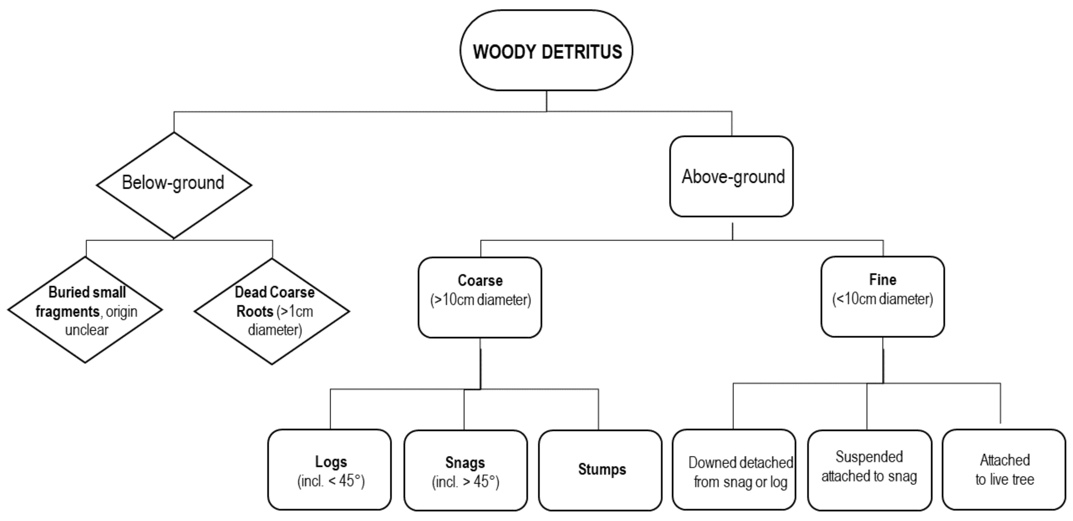
Table 1.
Main studies related to deadwood (standing or lying) identification through Airborne Laser Scanning (ALS) data (Corr.: correcteness, Compl.: completeness, Omiss.: omission, Comm.: commission ).
Table 1.
Main studies related to deadwood (standing or lying) identification through Airborne Laser Scanning (ALS) data (Corr.: correcteness, Compl.: completeness, Omiss.: omission, Comm.: commission ).
| Author | Aim | Seasonality | Site Type | Scanning Type | High Density (pts/m2) | Low Density (pts/m2) | DBH Threshold (cm) | Accuracy (%) | |
|---|---|---|---|---|---|---|---|---|---|
| Blanchard et al., 2011 [81] | U.S.A. | Downed logs | - | Mostly open area | Discrete return (DR) | 10.5 (20) | No | 25 | 73 |
| Lindberg et al., 2013 [82] | Sweden | Downed logs | Leaf-off | Conifer forest | DR | 69 | No | - | Corr.: 32 Compl.: 41 |
| Nyström et al., 2014 [83] | Sweden | Downed logs | Leaf-off | Conifer forest | DR | 65 | No | 6.9 | Corr.: 64 Compl.: 38 |
| Mücke et al., 2012 [75] | Germany | Standing dead trees, downed logs | Leaf-on/Leaf-off | Beech stand | Full waveform (FWF) | 21.8 (leaf-on) 16.9 (leaf-off) | No | 30 | |
| Mücke et al., 2013a [84] | Germany/Hungary | Downed logs | Leaf-off | Old-growth broadleaved forest | FWF | 29.4 (all) 10.9 (single/last) | No | 30 | Corr.: 75.6 Compl.: 89.9 |
| Polewski et al., 2014 [86] | Germany | Downed logs | Leaf-off | Mountain mixed forest | FWF | 30 | No | - | |
| Polewski et al., 2015 [72] | Germany | Downed logs | Leaf-off | Mountain mixed forest | DR (from FWF) | 30 | No | 10 | Corr.: 55–90 Compl.: 56–82 |
| Polewski et al., 2016 [87] | Germany | Downed logs | Leaf-off | Mountain mixed forest | DR (from FWF) | 30 | No | 10 | Corr.: 47–97 Compl.: 34–71 |
| Abalharth et al., 2015 [79] | U.S.A. | River logjams | - | Dense forest | - | 9–27 | No | - | Omiss.: 5 Comm.: 10 |
| Tanhuanpää et al., 2015 [103] | Finland | Downed logs/classification | Leaf-off | Urban conifer stand | - | 20 pulses | No | - | 97.8 (logs) 89 (classif.) |
| Bright et al., 2013 [62] | U.S.A. | Dead trees’ basal area | Leaf-on/Leaf-off | Different conifer forests | DR | No | 0.5–8.7 | - | 24.9–43.8 |
| Bater et al., 2009 [58] | U.S.A. | Standing dead trees class distribution | Leaf-on | Conifer forests | DR | No | < 1 | 10 | - |
| Casas et al., 2016 [76] | U.S.A. | Standing dead trees | - | Mixed landscape | DR | 19 | No | 10 | 84.8 |
| Polewski et al., 2015b [77] | Germany | Standing dead trees | Leaf-on | Mountain mixed forest | FWF + NIR imagery | 30–40 | No | - | 89 |
| DR (from FWF) | - | No | - | Corr.: 77.8 Compl.: 63.1 | |||||
| Yao et al., 2012a [70] | Germany | Classification live/dead trees | Leaf-on/Leaf-off | Mountain mixed forests | DR (from FWF) | 25 | No | 7 | 73 |
| Wing et al., 2014 [67] | U.S.A. | Standing dead trees | Leaf-on | Mostly conifer stands | DR | No | 6.9 | Live: 9 Dead: 12 | 40–60 (DBH <37 cm) 55–80 (DBH >37 cm) |
| No | 6.7 | Live: 9 Dead: 12 | >65 (DBH >37 cm) | ||||||
| Kobal et al., 2014 [106] | Slovenia | Snow/ice damages | Leaf-off | Mountain mixed forests | DR | ~200 points | No | - | - |
| Wallace et al., 2014 [107] | Australia | Crown pruning | Leaf-on | Eucalyptus plantation | Unmanned aerial vehicle (UAV) DR | 145–220 | No | - | - |
| Sherrill et al., 2008 [55] | U.S.A. | Coarse woody debris (CWD) | Leaf-off | Subalpine conifer stands | DR | No | 1.57–2.36 | All | - |
| Leaf-on | DR | No | 2.36 | All | - | ||||
| Keränen et al., 2015 [80] | Finland | Forest inventory | Leaf-on | Boreal mixed forest | DR | No | <1 | 3 | - |
| Maltamo et al., 2014 [41] | Finland | CWD | Leaf-on | Boreal mixed forest | DR | No | 2.8 | 5 | - |
| Pesonen et al., 2008 [54] | Finland | Standing/downed | Leaf-on | Spruce-dominated stands, aspen stands | DR | No | 0.5 | 5 | Standing: 78.8 Downed: 51.6 |
| Kim et al., 2009 [74] | U.S.A. | Standing dead tree | Leaf-on | Mainly conifer forest | DR | No | >6 | 10 | - |
| Martinuzzi et al., 2009 [52] | U.S.A. | Standing deadwood for habitat modeling | Leaf-on | Temperate conifer forests | DR | No | 1.95-m post spacing | 2.7 | 86–88 |
| Ackers et al., 2015 [112] | U.S.A. | Standing deadwood for habitat modeling | Leaf-on | Conifer-dominated forests | DR | 9 pulses with 4 returns | No | - | - |
© 2018 by the authors. Licensee MDPI, Basel, Switzerland. This article is an open access article distributed under the terms and conditions of the Creative Commons Attribution (CC BY) license (http://creativecommons.org/licenses/by/4.0/).
Share and Cite
MDPI and ACS Style
Marchi, N.; Pirotti, F.; Lingua, E. Airborne and Terrestrial Laser Scanning Data for the Assessment of Standing and Lying Deadwood: Current Situation and New Perspectives. Remote Sens. 2018, 10, 1356. https://doi.org/10.3390/rs10091356
AMA Style
Marchi N, Pirotti F, Lingua E. Airborne and Terrestrial Laser Scanning Data for the Assessment of Standing and Lying Deadwood: Current Situation and New Perspectives. Remote Sensing. 2018; 10(9):1356. https://doi.org/10.3390/rs10091356
Chicago/Turabian StyleMarchi, Niccolò, Francesco Pirotti, and Emanuele Lingua. 2018. "Airborne and Terrestrial Laser Scanning Data for the Assessment of Standing and Lying Deadwood: Current Situation and New Perspectives" Remote Sensing 10, no. 9: 1356. https://doi.org/10.3390/rs10091356
Note that from the first issue of 2016, this journal uses article numbers instead of page numbers. See further details here.