Development of Shoreline Extraction Method Based on Spatial Pattern Analysis of Satellite SAR Images

1
Department of Civil Engineering, The University of Tokyo, 7-3-1 Hongo, Bunkyo-ku, Tokyo 113-8656, Japan
2
Advanced Media, Inc., 3-1-4 Higashi-Ikebukuro, Toshima-ku, Tokyo 170-8630, Japan
*
Author to whom correspondence should be addressed.
Remote Sens. 2018, 10(9), 1361; https://doi.org/10.3390/rs10091361
Submission received: 25 July 2018
/
Revised: 21 August 2018
/
Accepted: 24 August 2018
/
Published: 27 August 2018
(This article belongs to the Special Issue Pattern Analysis and Recognition in Remote Sensing)
Abstract
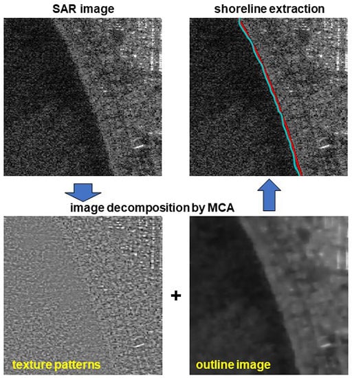
:The extensive monitoring of shorelines is becoming important for investigating the impact of coastal erosion. Satellite synthetic aperture radar (SAR) images can cover wide areas independently of weather or time. The recent development of high-resolution satellite SAR images has made observations more detailed. Shoreline extraction using high-resolution images, however, is challenging because of the influence of speckle, crest lines, patterns in sandy beaches, etc. We develop a shoreline extraction method based on the spatial pattern analysis of satellite SAR images. The proposed method consists of image decomposition, smoothing, sea and land area segmentation, and shoreline refinement. The image decomposition step, in which the image is decomposed into its texture and outline components, is based on morphological component analysis. In the image decomposition step, a learning process involving spatial patterns is introduced. The outline images are smoothed using a non-local means filter, and then the images are segmented into sea and land areas using the graph cuts’ technique. The boundary between these two areas can be regarded as the shoreline. Finally, the snakes algorithm is applied to refine the position accuracy. The proposed method is applied to the satellite SAR images of coasts in Japan. The method can successfully extract the shorelines. Through experiments, the performance of the proposed method is confirmed.
1. Introduction
In recent years, coastal erosion has led to the decline of sandy beaches. The decline of sandy beaches makes seawalls and roads along the coast more vulnerable to damage from waves. Coastal erosion is caused by various factors, such as decreases in the supply of sediment coming from rivers due to the construction of dams and changes in the flow of drifting sand caused by the construction of ports. Coastal erosion manifests as changes in the shoreline, and, therefore, wide area monitoring of shorelines has become more important for identifying the factors causing coastal erosion and for establishing effective countermeasures. Monitoring requires continuous observation in wide areas. Satellite imaging is suitable for monitoring owing to its low cost for taking images and its wide coverage area. Optical satellite images, however, cannot be used to observe the shoreline when they are taken at night or when the area is covered with clouds. On the other hand, images acquired by synthetic aperture radars (SARs) are more suitable for monitoring owing to the following characteristics: they can operate during the day and night, their observations are not influenced by the weather, and they can accomplish regular monitoring according to their orbit.
Research on automatic shoreline extraction from SAR images has been carried out. Lee and Jurkevich presented an early study on automatic shoreline extraction from satellite SAR images [1]. Because their research aimed to obtain the direction and position of the coastline for autonomous navigation and the determination of the geographical position of ships, the monitoring of shorelines was not taken into account for automatic extraction. Their method was sufficient for obtaining the direction and position of the coastline, but thin inlets could not be successfully extracted because of certain problems, such as speckle and low SAR image resolution. Methods for automatic shoreline extraction have been proposed since that research was published. These methods can be divided into two types of approaches: (1) extracting the shoreline as edges [2,3,4,5] and (2) classifying the sea and land areas and then extracting the shoreline as the boundaries between them [6,7,8].
In an approach of the first type, Mason and Davenport [2] used low-resolution images by taking the average pixel value in a 4 × 4 region to eliminate speckle and reduce the necessary calculation time. Edge extraction was then applied to these low-resolution images [9], and the results were superimposed on the images with their original resolution. Finally, the snakes algorithm, proposed by Kass et al. [10], was applied to determine the final shoreline. However, there were limitations on the settings for edge determination and for the snakes algorithm due to speckle, and extraction errors occurred in many parts. Liu and Jezek [3] proposed eliminating the speckle first and then applying edge emphasis and the Canny filter [11] as an edge extraction method. Results were acquired through threshold processing. This method was applied to SAR images of Antarctica as an experiment, but it was difficult to extract shorelines if there were obstacles, such as icebergs, in the coastal area. Wang and Allen [4] and Asaka et al. [5] used observation data from the PALSAR (ALOS “Daichi”), which is a satellite SAR that was launched by Japan. Wang and Allen [4] used the images obtained by outputting the maximum and the minimum pixel values within a specific filter size and taking the difference. They exploited the fact that this difference increases in the vicinity of the shoreline. The influence of speckle is suppressed by outputting the maximum and the minimum values within the filter size. Asaka et al. [5] selected the edges using a one-dimensional Laplacian of Gaussian (LoG) filter to obtain sea/shoreline/land training data for extracting shorelines. In these experiments, it was possible to extract the shoreline in general. However, if the shoreline was unclear because of speckle, there were some cases in which the shoreline could not be accurately extracted.
In the other type of approaches, the sea and land areas are first classified and then the boundary between them is extracted as the shoreline. Zhang et al. [6] performed segmentation exploiting the fact that the distribution of pixel values in sea areas is more homogeneous than in land areas after performing smoothing for speckle removal. Using this method, relatively homogeneous land areas and non-homogeneous sea areas may be erroneously classified, but they can be removed based on their small size. Nunziata et al. [7] used multi-polarized SAR images. By exploiting the fact that the correlation between VV and VH (the first capital letter indicates the angle of transmission while the second letter denotes the angle of reception with H and V, horizontal and vertical angles, respectively) is more remarkable than single-polarized scattering intensity images, sea and land areas were segmented. Vandebroek et al. [8] monitored the changes in shorelines to evaluate the results of a beach nourishment project (Sand Motor) on the west coast of the Netherlands. In approximately 55% of the images, they were able to effectively extract the shoreline. Ultimately, they concluded that coastal dynamics could be evaluated only for changes in the order of tens of meters.
The spatial resolution of the first satellite SAR launched for the observation of Earth’s oceans (called Seasat) was approximately 15 to 30 m, while that of satellite SARs launched in recent years is approximately 3 to 5 m. For shoreline monitoring, the accuracy required depends on the spatial resolution of the satellite SAR images used. The erroneous extraction of patterns (such as wave crest lines and sandy beaches) cannot be ignored when working with SAR images of higher resolution. SAR images with coarse resolution or small influence of waves were used in most previous research. Therefore, there are few studies mentioning the erroneous extraction due to wave crest lines or sandy beach patterns. Vandebroek et al. [8] extracted shorelines using TerraSAR-X images with a resolution of 3 m for shoreline extraction. The influence of the waves (in the sea area) and the brightness of sandy beaches (in the land area) were pointed out as factors of failure in extraction. Accordingly, when conducting wide-area monitoring with a unified method, countermeasures against wave crest lines and sandy beach patterns are essential.
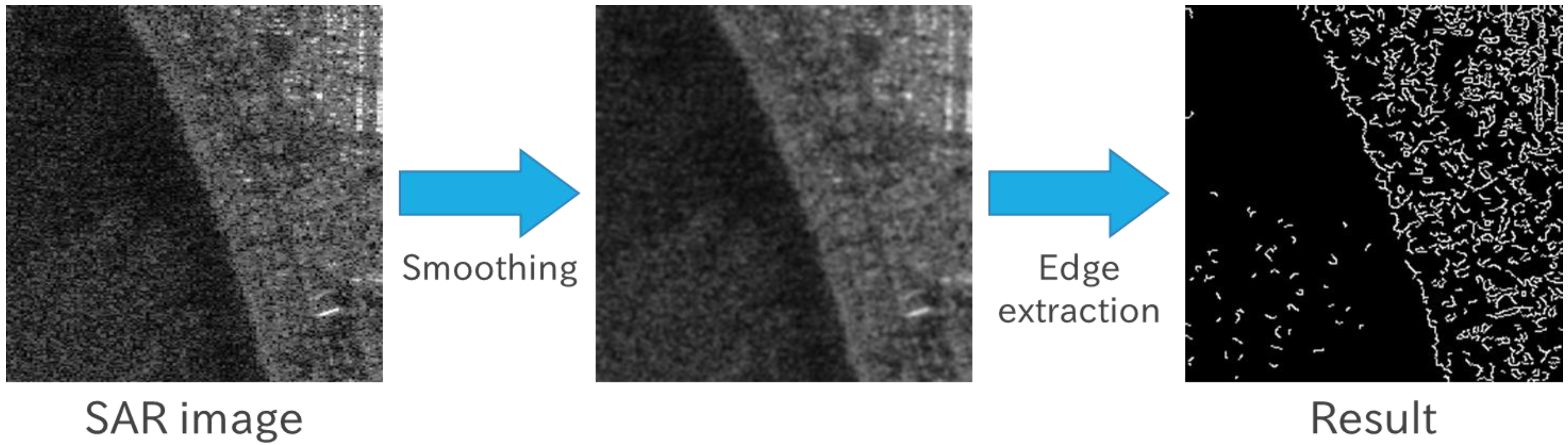
Smoothing filters, such as the Gaussian filter, are effective for removing speckle. However, parts of the wave crest lines and sandy beaches are often extracted incorrectly as edges. Figure 1 shows an example that the ordinary method has a limitation against the effect of textures such as wave crest lines and sandy beaches. Wave crest lines and sandy beaches seem to have different spatial patterns from that of speckle. It is difficult to remove them in the same way as when removing speckle. On the other hand, they seem to repeat similar patterns. Speckle is considered to be a section where pixel values change locally, while the shoreline is considered to be a part where large changes of pixel values are linearly connected. By separating speckle, wave crest lines and sandy beach patterns from SAR images and using only components related to the shoreline, shorelines can be extracted with high accuracy. The proposed method in this paper deals with image decomposition to separate such texture patterns from original SAR images.
The term “shoreline” in this paper is used according to the Vandebroek et al. [8]. It is defined as the instantaneous intersection of water and land at the time of the SAR observations.
The SAR data used in this research are described in Section 2.1. The principle of the proposed method and our method of accuracy verification are explained in Section 2.2. Our results and discussion are presented in Section 3. Finally, Section 4 concludes this paper.
2. Materials and Methods
2.1. Input Data
We used the SAR data observed by the L-band synthetic aperture radar PALSAR-2, which is installed in a satellite called ALOS-2, launched by the Japan Aerospace Exploration Agency (JAXA) in 2014. Most of the SAR scenes were obtained with the “Ultra-fine” observation mode (single look) that has a spatial resolution of 3 m. Full polarization scenes were obtained under the observation mode of “High-sensitive”, with a spatial resolution of approximately 5 m in the range direction and 4 m in the azimuth direction. The observation area of each single SAR scene under the “Ultra-fine” mode is 50 km by 70 km (range by azimuth), while the “High-sensitive” mode has a slightly narrower observation extent in the range direction. Because the higher resolution was required in this study, only HH-polarized waves (“Ultra-fine” mode) were used, and multi-polarized observation data were not used in combination. PALSAR-2 data have a processing level indicating how it was processed from the raw data. In this research, we used processing levels 1.1 and 1.5. Processing level 1.1 consists of complex-valued data obtained after range compression and azimuth compression and includes phase information in addition to intensity. The horizontal direction of these SAR images is the slant range direction. On the other hand, processing level 1.5 contains only intensity information, but the horizontal direction in this case is the ground range direction (after map projection).
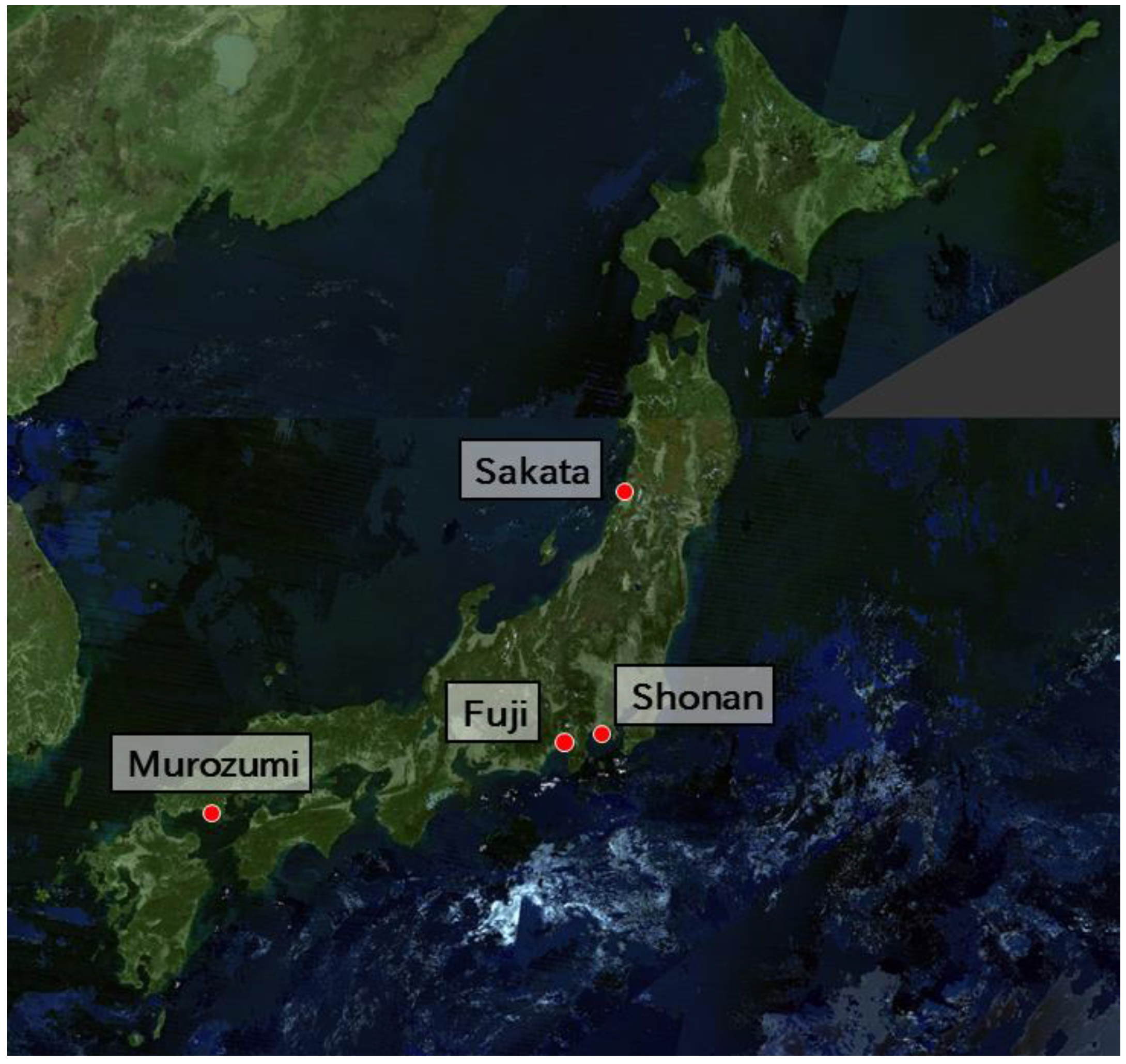
The coasts of interest are shown in Table 1 and Figure 2. In order to measure the actual position of the shoreline, on-site observations were conducted for each coast. We used a GARMIN GPSmap 60CSx (Handy GPS) (Olathe, KS, USA) to measure the shoreline. The accuracy of the GPS is ±3 m, which is almost equal to the resolution of SARs. On-site observations were made close to the planned time for satellite observation so that the position of the shoreline observed from the satellite coincided with our on-site observations. Whenever the time of an on-site observation differed from that of the satellite observation, that on-site observation was made in a time such that the tide level during the satellite observation coincided with the tide measured on-site, either several days before and after. In Sakata, the tide level during the on-site observations was not consistent with the tide level during the satellite observation, and thus the SAR images of Sakata were excluded from our quantitative accuracy verification. In this research, we verified the accuracy of the proposed method by comparing the shoreline extracted using it with the GPS data of the on-site observations. The method for accuracy verification is described in Section 2.2.5. The SAR images were trimmed to 256 × 256 pixels.
2.2. Methods
The proposed method consists of four steps. As mentioned in Section 1, we focused on spatial patterns in SAR images. The shoreline is considered as the part of the image where large changes of pixel values are linearly connected, and speckle is considered to be the parts where the pixel values change locally. Wave crest lines and sandy beaches seem to have similar repeating patterns. By using a sparse-modeling technique [13], images including only smooth components, such as the shoreline (outline), and images including speckle and spatial patterns (texture) are decomposed. Only the outline component is used in subsequent steps.
The outline image is smoothed using the non-local means filter. Then, the image is segmented into sea areas and land areas (hereinafter called “sea–land binarization”), and the boundary is extracted as the shoreline. For the sea–land binarization process, the graph cuts technique is applied. The graph cuts technique can reflect the distribution of pixel values and their difference with surrounding pixel values. Finally, the extracted shoreline is refined using the active contour method.
In the following sections, the principle of each method will be explained step by step.
2.2.1. Image Decomposition Based on Spatial Patterns
First, image decomposition is applied based on the differences in spatial patterns, such as the shoreline, speckle, wave crest lines, and sandy beaches in the SAR images. Because the objective of this research is the extraction of shorelines, it is necessary to decompose the source data into images containing only the components related to smooth changes, such as shorelines, and images containing speckle and other spatial patterns. We assumed that both types of images are sparsely generated from different models [14]. This sparsity means that most of the elements of the feature vectors representing the image are equal to zero. Such techniques based on sparsity are called sparse modeling techniques. Morphological component analysis (MCA) [15,16,17] is one of such sparse modeling techniques, and it is suitable for our image decomposition problem. MCA requires a dictionary, which is a matrix of parameters representing spatial patterns of image intensity. The dictionary should be determined beforehand. In our research, a dictionary was learned using small patches for each image. Then, each SAR image was decomposed into an image including only components related to smooth changes, such as the shoreline (outline), and an image including speckle and spatial patterns (texture). The learning process and the image decomposition were accomplished as follows.
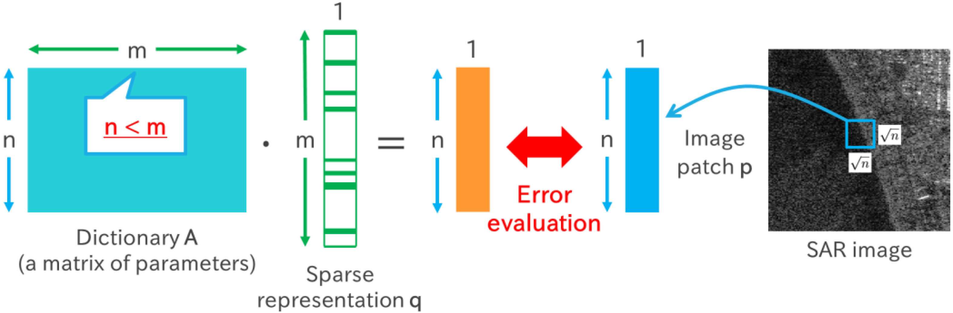
Let be an image of size pixels and composed of the outline component and the texture component (i.e., ). Let us consider a small patch of size pixels , where is a column vector in which pixel values are arranged in a row. These patches have a dictionary . Moreover, each patch has a corresponding sparse representation , which satisfies
where is a parameter indicating an allowable error. For ,
where is called the “ norm”. When ( norm),
This represents the number of non-zero elements of . The number of non-zero elements of has the constraint . When is set to a small value, becomes sparse (most elements are zero), and its features can be expressed with just a few variables [18]. The dictionary and sparse representations are learned so that the error becomes or less in all patches (Figure 3).
Image is shifted in steps of one pixel from the upper left corner of the image, and patches are clipped by allowing duplication. Each patch is denoted as , where is the number of patches. Although the number of pixels in the image is , the number of patches is slightly less than because of the size of the patch. Additionally, has a one-to-one correspondence with coordinates in the image. Here, the operator denoted the process of clipping the -th patch (i.e., ). Let be the sparse representation corresponding to . Thus, the constraint equation is as follows:
In Equation (4), sparse representation and dictionary are unknown. In order to estimate these factors, the initial value of dictionary is set to a two-dimensional redundant DCT (discrete cosine transform) dictionary, and and are alternately updated. According to the maximum a posteriori estimation, is updated by solving Equation (5), which is an independent optimization problem for each patch (where is a constant) [19]. The approximate solution of Equation (5) can be calculated using the orthogonal matching pursuit (OMP) method [20]:
After is calculated, dictionary is updated using the K-SVD (singular value decomposition) algorithm [21]. The dictionary can be learned from the image itself, including noise, by alternately and repeatedly updating and . The learning process does not need any training data, which represents a major advantage of the proposed method.
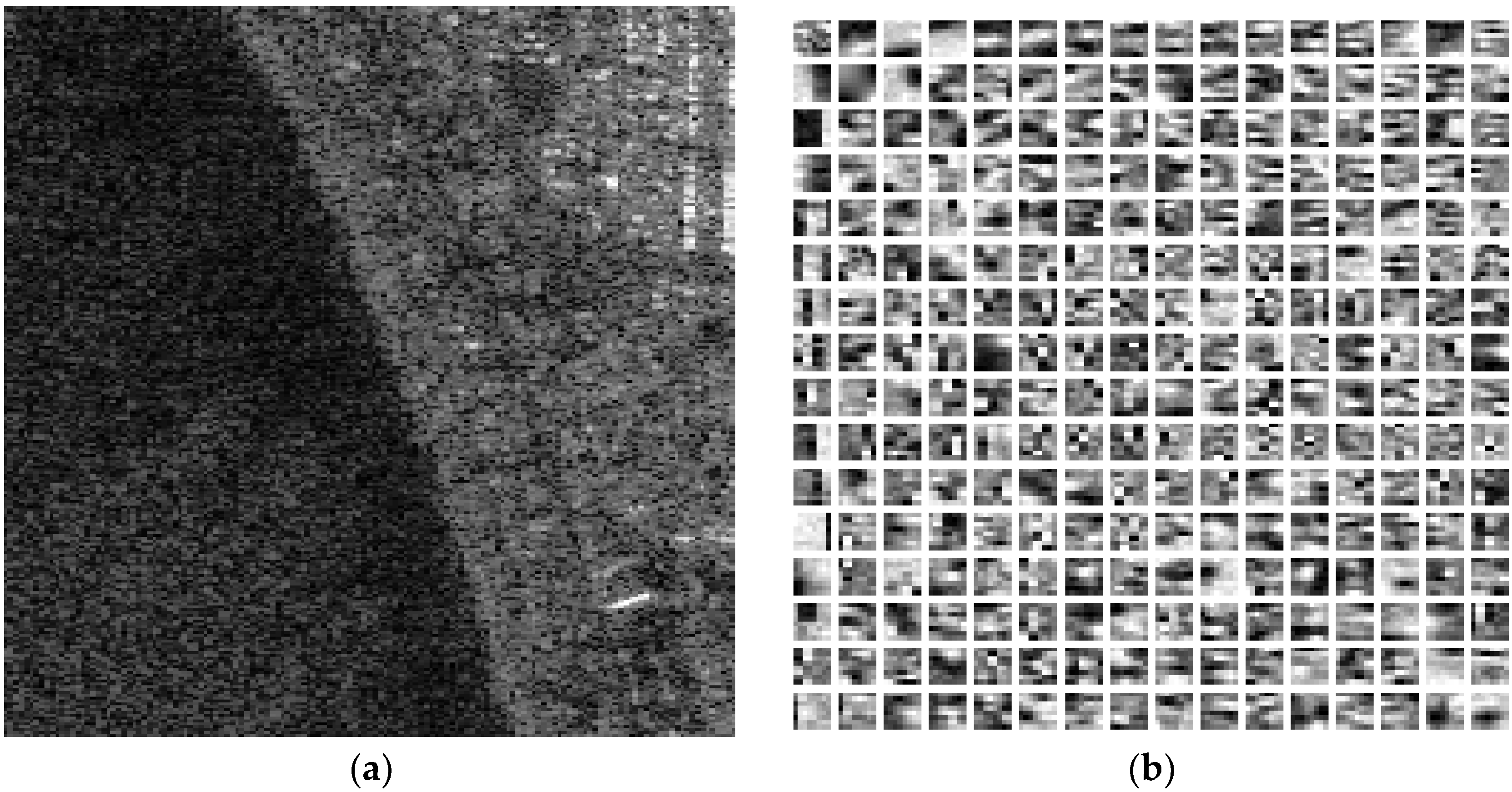
After the learning process, dictionary is decomposed into the outline and texture dictionaries, and these two dictionaries are used for image decomposition. The learned dictionary has atoms (columns) for outline () and texture (), and both are mixed in the dictionary. Figure 4 shows a dictionary after learning with an SAR image of the Murozumi coast. The patch size used was 8 × 8, and the size of the redundant DCT dictionary was 64 × 256 according to Elad et al. [16]. Each small square corresponds to one atom. The number of iterations for learning was set to 25 times by checking the convergence.
From Figure 4b, it can be seen that the dictionary is divided into atoms that capture smooth changes and atoms that capture stripe patterns. The former corresponds to atoms of the outline, and the latter corresponds to atoms of texture. To decompose them, atom is considered as a patch of size , and the following “activity measure” is calculated. The component of the atom considered to be a patch is represented as :
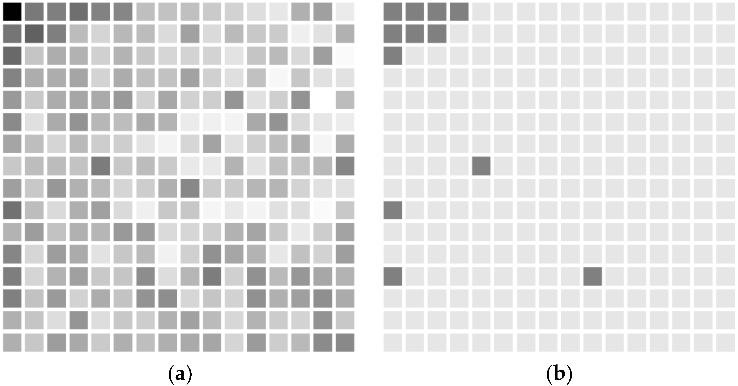
This activity measure is the sum of differences of adjacent elements in the column vector. In atoms of the outline, the difference with adjacent elements is small, whereas, for texture atoms, it is large. The activities are normalized so that the maximum value becomes 1. By applying thresholding to the activity values, the atoms are assigned to either the texture or outline dictionaries. Figure 5a shows the activity of the atoms, and the corresponding assignment to either dictionary is shown in Figure 5b, for a threshold value of 0.5. In Figure 5a, activity close to 0 (outline) is colored black, while activity close to 1 (texture) is colored white. In the assignment, shown in Figure 5b, gray squares depict atoms that are determined to be the outline, while white ones depict atoms that are determined to be texture. Most atoms are classified as texture.
When dictionary is decomposed into and , can also be allocated according to the atoms. Thus, outline image and texture image can be calculated. The dictionary can take into account multiplicative nature of the speckle. The atoms in the dictionary correspond to various patterns of the texture. Figure 6 shows the results after decomposing the SAR image of the Murozumi coast into the outline and texture images. The texture image was normalized by its pixel value for easy viewing.
In this research, the patch size used was 8 × 8 pixels, and the size of the redundant DCT dictionary was 64 × 256 according to Elad et al. [16]. The number of iterations for learning was set to 25 times by checking the convergence. To reduce memory use, the number of patches used for one iteration of the K-SVD algorithm was set to 1/10 of the whole, and the patches were randomly extracted in each iteration. When the number of patches used was more than 1/10 of the whole, the calculation was not be completed due to lack of memory. The allowable error was (: patch size), and the number of non-zero elements in the sparse expression was . The threshold for the activity measure for separating between outline and texture was 0.5.
2.2.2. Smoothing
Because the outline image still has noise even after image decomposition is applied, a smoothing filter is subsequently applied to the image for a more stable accuracy. For smoothing the images, calculating the weighted average of neighboring pixels, such as when using a Gaussian filter, is a popular method. However, for SAR images of coasts, it is desirable to increase the weight for the parts where the distribution of pixel values is similar, even in a section away from the target one, such as the continuous coast. The non-local means filter is appropriate for this purpose [22], and we adopted it in this work as our smoothing filter. We used a simple non-local means filter. The more sophisticated approaches such as Deledalle et al. [23] have been proposed. The applications of such approaches are considered as the future work.
The Gaussian filter uses only the surrounding pixels of the target pixel to apply normal-distribution weighting. On the other hand, the non-local means filter takes all pixels in the image [24]. The weight of target pixel pi is calculated by using its neighboring pixels pj and separating image patch qj at the center qi. The pixel value is expressed by I( ·) in the following equation:
where is a normalization term and is a parameter;
2.2.3. Sea–Land Binarization
The smoothed outline image is classified into two types (sea–land binarization) for each pixel, and the boundary is extracted as the shoreline. Spatial filtering and region growing are popular methods for extracting such boundaries, but sometimes the shoreline is not extracted well (Figure 7). The reason behind this is that these methods process local data and do not capture the global features of SAR images. Therefore, we applied the graph cuts technique [25], which can reflect the distribution of pixel values and the differences with neighboring pixel values.
Directed graphs are constructed between the pixels of an image [26]. In such graphs, the pixels are taken as nodes, and these nodes are connected by edges. Each edge has a cost, which will be defined later. As shown in Figure 8, directed edges (S → pixels, pixels → L) are constructed between neighboring pixels and the newly considered initial node S and terminal node L. Binarization is performed by dividing the graph into subset graphs called graph cuts. Among the possible patterns of graph cuts, a cut minimizing the sum of the cost is called a mini-cut [27]. The smaller the edge cost is, the weaker the binding as a region is. Hence, the edges whose cost is small tend to become part of the final edge [28]. The mini-cut problem can be solved by using the NetworkX library.
The cost of the edges for the graph cuts technique are defined by using the histograms of the distribution of pixel values of the sea side (S) and the land side (L) beforehand. In the proposed method, pixels on the sea and land sides are designated by user (only one pixel in each side), and the average and the standard deviation values are determined from the pixel values of the neighboring pixels. Then, the normal distributions with the obtained average and standard deviation values are defined as the respective histograms, hS and hL. The histograms are normalized to 1 at a pixel value range of 0 and 255. The costs of the edges between S and L, and pixel p (pixel value is I(p)), CS and CL, respectively, are defined as follows:
The cost of the edges between adjacent pixels p and q, C(p, q), is defined as follows:
where and are parameters.
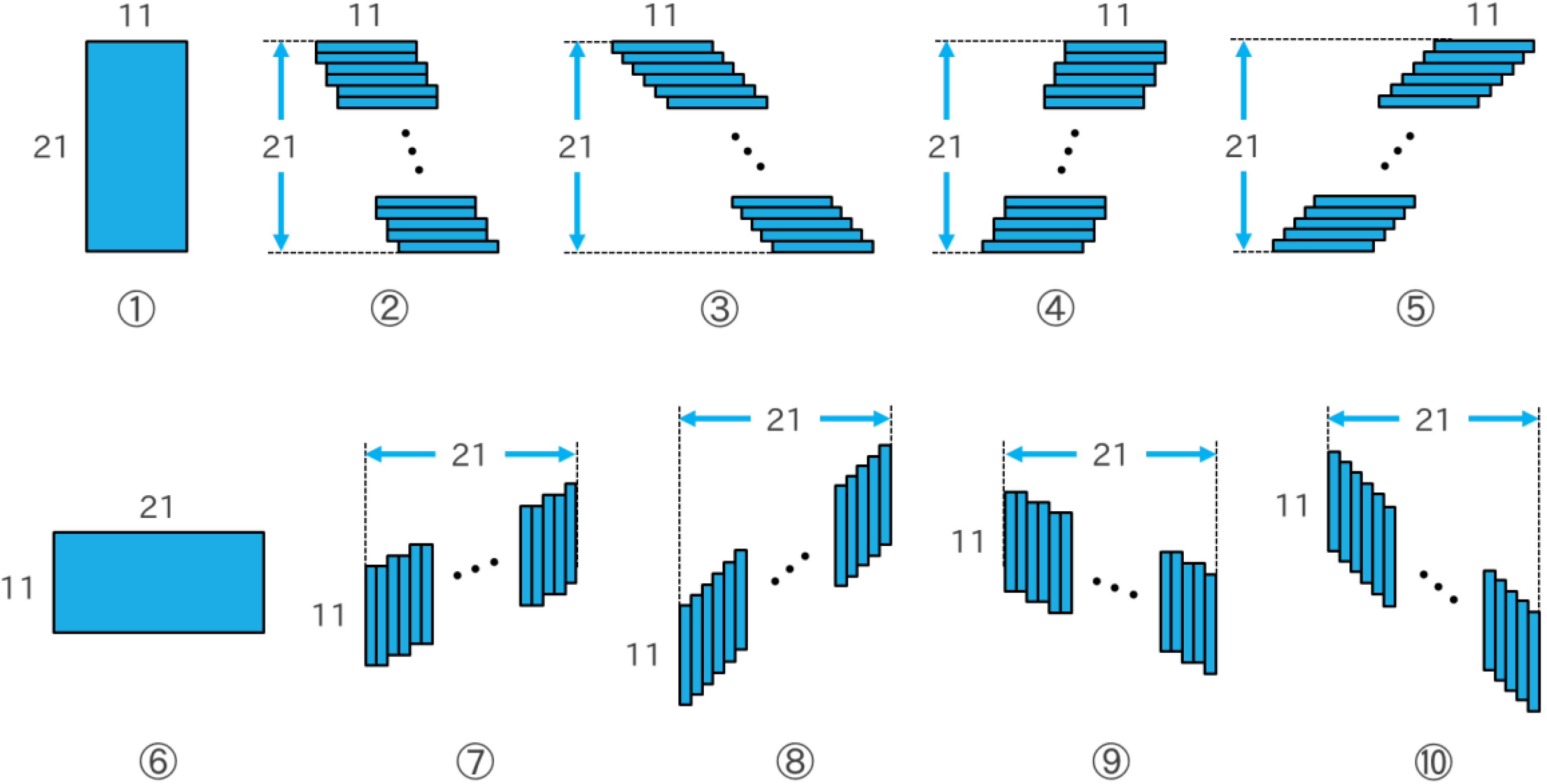
The peripheral area of a designated pixel is defined to be one of the ten types shown in Figure 9. The designated pixel is in the center of the area. Types 1 and 6 are normal rectangular areas, while types 2, 4, 7, and 9 are parallelogram-shaped regions, where the short side is shifted by one pixel every two pixels in the long side direction. Types 3, 5, 8, and 10 are parallelogram-shaped regions where the short side is shifted by one pixel for each pixel in the long side direction. The average and standard deviation values are calculated for these region types. The region type for which the standard deviation is smallest is adopted as the peripheral area. According to the peripheral area adopted, the average and standard deviation values of the sea and land regions are then calculated. The region with the smallest standard deviation is regarded to be the least influenced by the land area (in the case of the sea area), and vice versa.
2.2.4. Refinement of the Extracted Shoreline
The graph cuts technique in the previous section uses only the pixel values of the image. Additional information, such as the gradient of pixel values and the smoothness of boundary lines, led to finer shoreline extraction results. Therefore, the snakes algorithm [10] was additionally applied for refining the shoreline extraction method. The snakes algorithm defines a curve on the image and modifies the shape of the curve to minimize the energy function. We can obtain the point sequence of a boundary line v(s) = [x(s), y(s)] (s is a certain distance along the line, ). The energy function Esnake consists of the internal energy Eint and the image energy Eimage:
The internal energy includes the length and curvature of the line:
where and are weight constants. This means that shorter and smoother lines are a better solution. The image energy includes the pixel’s intensity Eline = −I(x,y), gradient of the intensity Eedge = , and the terminal condition Eterm:
where w represents the weight. According to the image energy, lines with higher intensity and gradient tend to be selected.
2.2.5. Method for Accuracy Verification
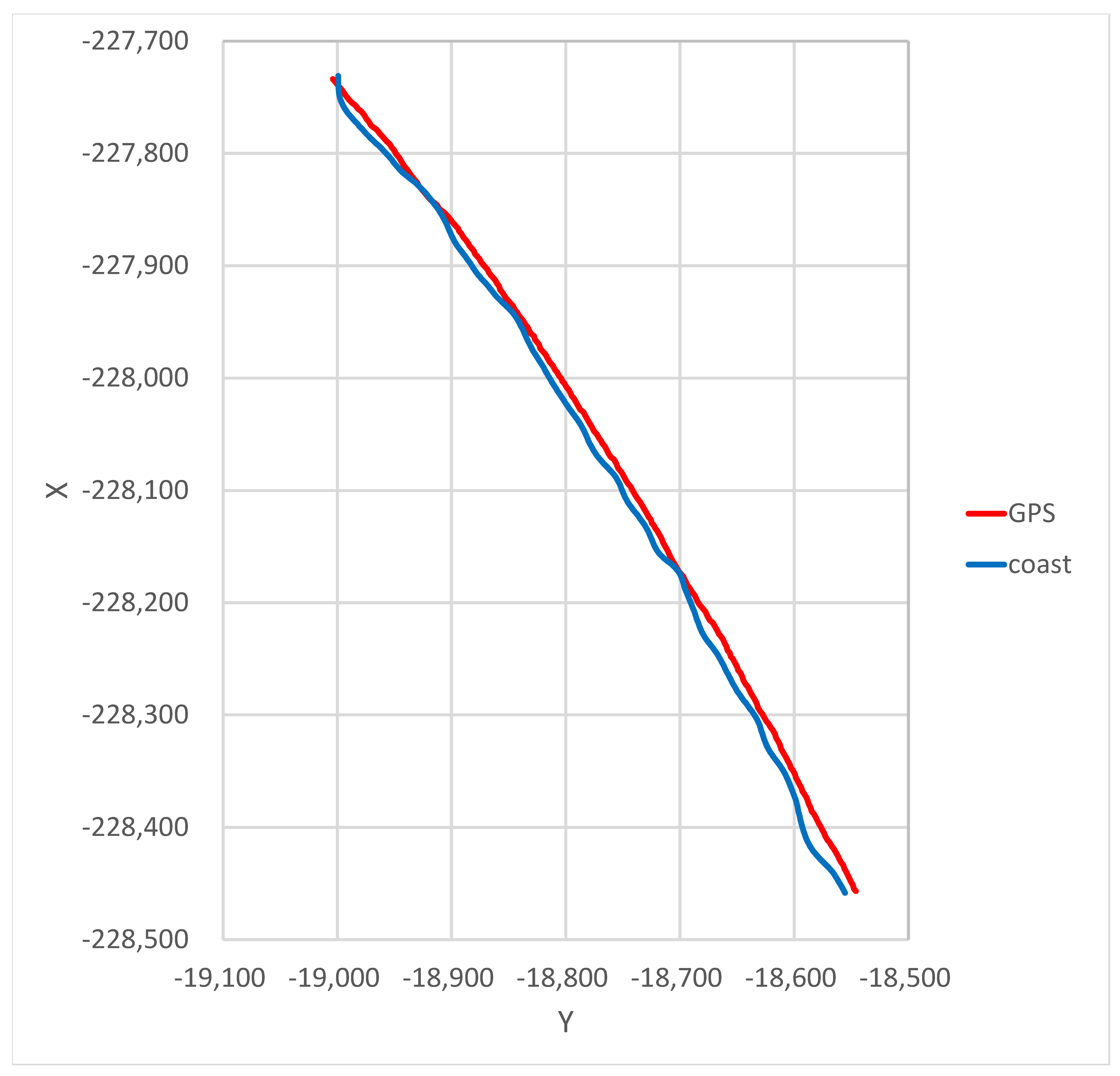
The shoreline data extracted by the graph cuts technique and the snakes algorithm are a set of coordinates of points shown in the coordinate system of the SAR image, with the pixel at the upper-left corner of the image being (0, 0), the right direction being the positive direction of the x-axis, and the downward direction being the positive direction of the y-axis). In our method, the image coordinates of each shoreline point are converted to a plane rectangular coordinate system. GPS data are indicated by the longitude and latitude at each point and are also converted to a plane rectangular coordinate system. After converting each point of the extracted shoreline and GPS data into a plane rectangular coordinate system, interpolation is performed with a straight line between the points. Figure 10 shows an example of this interpolation process. Accuracy is evaluated by drawing a normal line from the line of the GPS data and calculating the distance to the intersection with the extracted shoreline. The average of these distances is used as an evaluation index of accuracy. Points to be evaluated are arranged at 5-m intervals in a specific direction (the direction of the x-axis was used in the example shown in Figure 10) on the GPS data.
3. Results and Discussion
3.1. Accuracy Verification of the Shoreline Extraction Method
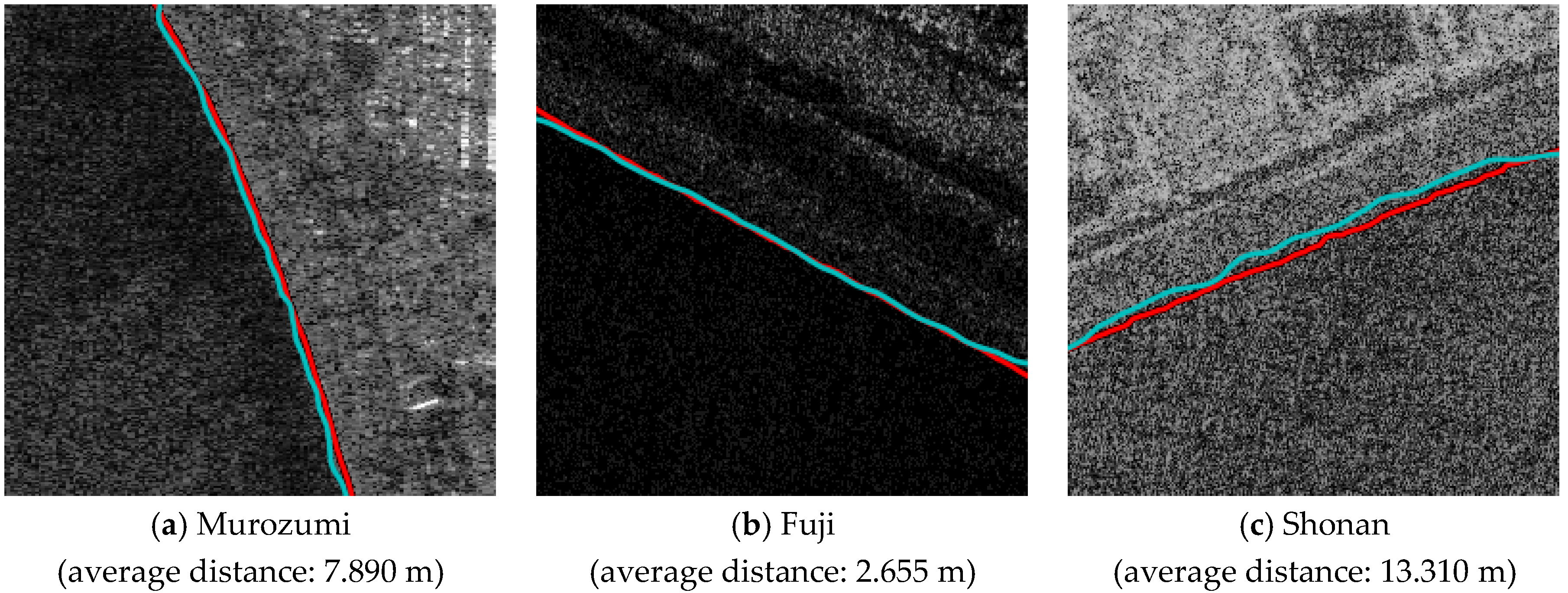
The proposed method was applied to SAR images of the Murozumi, Shonan, and Fuji coasts (shown in Table 1), and the resulting accuracies were verified with GPS data. We used a GARMIN GPSmap 60CSx (Handy GPS) to measure the shoreline as described in Section 2.1. The accuracy of the GPS is ±3 m, which is almost equal to the resolution of SARs. On-site observations were made close to the planned time for satellite observation so that the position of the shoreline observed from the satellite coincided with our on-site observations. The shoreline length of interest in this study is approximately 2 km. It took less than 20 min for the on-site observations. We confirmed that the tidal effect was quite small. Figure 11 shows the shoreline extracted using the proposed method, GPS data, and the average distance between the two. Accuracy is evaluated by drawing a normal line from the line of the GPS data and calculating the distance to the intersection with the extracted shoreline. The average of these distances is used as an evaluation index of accuracy, as described in Section 2.2.5.
On the Murozumi and Fuji coasts, the shorelines were successfully extracted with errors within only several meters on average, namely almost one pixel. Additionally, experts in coastal engineering determined that the resulting accuracy was sufficient for shoreline monitoring. On the other hand, the error was larger on the Shonan coast. As shown in Figure 11c, because the extracted shoreline was closer to the land side than the GPS data, we infer that the sandy beach could not be clearly determined. The reason is that the constituent particle diameter of that sandy beach is smaller than that of the Fuji coast. Another reason is that the off-nadir angle (ONA) of the image is larger than that of the Murozumi coast.
Figure 12 shows the results using the method proposed by [8], and GPS data. To improve visibility, results after sea–land binarization are depicted. On the Murozumi and Shonan coasts, the shoreline extraction obviously failed. On the Fuji coast, the clustering (k-means) could not be applied due to poor results of smoothing (Wiener filter). According to these results, effectiveness of the proposed method can be confirmed.
We also conducted a sensitivity analysis of the parameters. The important parameters are the number of non-zero elements in the sparse expression , the allowable error , the patch size, and the dictionary size. We applied the proposed method with the various parameter values to SAR image of the Murozumi coast. The results are shown in Table 2. The shoreline could be extracted with an error of only several meters on average with the same level. The differences of the average distances were much less than the resolution of SARs. These results indicate that the proposed method is robust to the parameter values.
3.2. Validation Using SAR Images with Breakwaters
As an example for verification using SAR images with obstacles in the sea area, the proposed method was applied to scenes with breakwaters. The original image and the experimental results are shown in Figure 13. The part that appears white surrounded by the blue dotted line in Figure 13a represents the breakwaters.
Although the distance from the GPS data at the lower end of the image was large, shorelines were extracted with an error of approximately 5 m at other places where there were breakwaters. However, when the distance between the sandy beach and the breakwaters was short, the shoreline could not be extracted well in some cases. Smoothing of the whole image makes extraction at highly detailed parts more difficult. Further experiments are needed to determine how much distance (pixels) away from the shoreline can be extracted.
3.3. Validation Using SAR Image with Wave Crest Lines
We also examined whether shorelines could be extracted from SAR images of Sakata with wave crest lines. The original image and the experimental results are shown in Figure 14.
3.4. Verification on Dictionary Sharing
A dictionary learned with a certain SAR image can be applied to other SAR images, and the outline and texture can be decomposed. When dictionaries can be shared, the learning process can also be shared between images. As a result, the time required for dictionary learning can be reduced, making the method much more efficient. We conducted experiments on the following types of approaches and verified the resulting accuracies (we calculated the average of the distance). The results are shown in Table 3:
- Type 1: Use a dictionary learned from another part of the same SAR scene,
- Type 2: Use a dictionary learned from a SAR image of another coast.
Type 1 shows that shorelines can be extracted with the same accuracy as when learning from the input images for any SAR image. However, regarding type 2, when extracting the shoreline of Shonan using Fuji’s dictionary in particular, the accuracy of the proposed shoreline extraction method deteriorated (Figure 16).
The SAR image of the Fuji coast is different from the others in characteristics such as the blackness of the sea area and indistinctive speckle. Hence, Fuji’s dictionary did not match well with the other SAR images.
These results show that dictionary sharing is sufficiently possible in the same SAR scene. Therefore, it is possible to learn a dictionary with a part of a certain SAR image and extract the shoreline using that dictionary for the entire image. This reduces the time required for dictionary learning and leads to more efficient calculations.
4. Conclusions
In this paper, a new shoreline extraction method was presented. The proposed method consists of image decomposition, smoothing, sea and land area segmentation, and shoreline refinement. The image decomposition step is based on morphological component analysis (MCA). MCA can decompose SAR images into a texture image, which includes speckle and spatial patterns, and an outline image. For this decomposition step, a learning process for spatial patterns (dictionary) is introduced. The learning process does not need any training data, and it can be performed automatically, which is one of the major advantages of the proposed method. The outline image is used in the subsequent steps. This image is smoothed using a non-local means filter. Then, it is segmented into sea and land areas using the graph cuts technique. The boundary between the two areas can be regarded as the shoreline. Finally, the snakes algorithm is applied to refine the position accuracy of the extracted shoreline.
The proposed method was applied to SAR images of the Murozumi, Shonan, Fuji, and Sakata coasts. The extraction accuracies were verified by calculating the distance between the shoreline extracted using the proposed method and the shoreline obtained via on-site observations using GPS. Although the errors were higher on the Shonan coast owing to the particle size of the sand there and the off-nadir angle at the time of the SAR observations, the shorelines could be extracted with an error of only several meters on average at the Murozumi and Fuji coasts. These results indicate that the proposed method is useful for highly accurate coastline monitoring. To check for the feasibility of applying our method in various situations, it was also applied to SAR image scenes with breakwaters and wave crest lines. In the case of breakwaters, the results confirm that the shorelines can be extracted if there is a certain minimum distance between the breakwaters and the sandy beach. In the case of wave crest lines, the results show that automatic extraction of shorelines is possible depending on certain conditions, such as the observation direction of the SAR. Through the experiments, several factors such as constituent particle diameter of the sandy beach, off-nadir angle of the image, foreshore slope, distance between the sandy beach and the breakwaters can be considered as the influencing factors to the results.
The effects of dictionary sharing for MCA was also examined, considering the efficiency of the method. Dictionaries were applied to other images in the same SAR scene and in different SAR scenes, and the accuracies of the extracted shorelines were evaluated. The results show that shoreline extraction is possible without degrading the accuracy if the dictionary is shared within the same SAR scene. Therefore, by learning the dictionary with only a part of the SAR image and using that dictionary for the whole image to extract the shoreline, it is possible to apply the proposed method efficiently.
As future work, the application of the proposed method for various types of SAR images will be considered. Through additional experiments, a stability analysis can be carried out for accuracy improvement. To perform such a stability analysis, the size of the image patches and the dictionaries used in the MCA step can also be examined. Furthermore, we will consider using SAR data from multiple polarized waves and bands. We expect these improvements to contribute to more accurate and stable coastline monitoring.
Supplementary Materials
Supplementary File 1Author Contributions
T.F. conceived the idea of the study and designed it. T.O. conducted the experiments. All authors contributed equally, analyzed the data, and prepared the manuscript.
Funding
This research was funded by the Research Grant in River and Sabo Fields in 2016–2017, provided by the Ministry of Land, Infrastructure, Transport and Tourism.
Acknowledgments
The authors would like to thank Tajima (University of Tokyo) for his useful comments from a coastal engineering point of view.
Conflicts of Interest
The authors declare no conflict of interest. The funders had no role in the design of the study; in the collection, analyses, or interpretation of data; in the writing of the manuscript, nor in our decision to publish the results.
References
- Lee, J.S.; Jurkevich, I. Coastline detection and tracing in SAR images. IEEE Trans. Geosci. Remote Sens. 1990, 28, 662–668. [Google Scholar]
- Mason, D.C.; Davenport, I.J. Accurate and efficient determination of the shoreline in ERS-1 SAR images. IEEE Trans. Geosci. Remote Sens. 1996, 34, 1243–1253. [Google Scholar] [CrossRef]
- Liu, H.; Jezek, K.C. Automated extraction of coastline from satellite imagery by integrating Canny edge detection and locally adaptive thresholding methods. Int. J. Remote Sens. 2004, 25, 937–958. [Google Scholar] [CrossRef]
- Wang, Y.; Allen, T.R. Estuarine shoreline change detection using Japanese ALOS PALSAR HH and JERS-1 L-HH SAR data in the Albemarle-Pamlico Sounds, North Carolina, USA. Int. J. Remote Sens. 2008, 29, 4429–4442. [Google Scholar] [CrossRef]
- Asaka, T.; Yamamoto, Y.; Aoyama, S.; Iwashita, K.; Kudou, K. Automated method for tracing shorelines in L-band SAR images. In Proceedings of the 2013 Asia-Pacific Conference on Synthetic Aperture Radar, Tsukuba, Japan, 23–27 September 2013; pp. 325–328. [Google Scholar]
- Zhang, D.; Gool, L.V.; Oosterlinck, A. Coastline detection from SAR images. IEEE Geosci. Remote Sens. Symp. 1994, 4, 2134–2136. [Google Scholar]
- Nunziata, F.; Buono, A.; Migliaccio, M.; Benassai, G. Dual-polarimetric C- and X-band SAR data for coastline extraction. IEEE J. Sel. Top. Appl. Earth Obs. Remote Sens. 2016, 9, 4921–4928. [Google Scholar] [CrossRef]
- Vandebroek, E.; Lindenbergh, R.; van Leijen, R.; de Schipper, M.; de Vries, S.; Hanssen, R. Semi-automated monitoring of a mega-scale beach nourishment using high-resolution TerraSAR-X satellite data. Remote Sens. 2017, 9, 653. [Google Scholar] [CrossRef]
- Touzi, R.; Lopes, A.; Bousquet, P. A statistical and geometrical edge detector for SAR images. IEEE Trans. Geosci. Remote Sens. 1988, 26, 764–773. [Google Scholar] [CrossRef]
- Kass, M.; Witkin, A.; Terzopoulos, D. Snakes: Active contour models. Int. J. Comput. Vis. 1988, 1, 321–331. [Google Scholar] [CrossRef] [Green Version]
- Canny, J. A computational approach to edge detection. IEEE Trans. Pattern Anal. Mach. Intell. 1986, 6, 679–698. [Google Scholar] [CrossRef]
- GSI Maps. Available online: https://maps.gsi.go.jp/ (accessed on 16 March 2018).
- Tibshirani, R. Regression shrinkage and selection via the lasso. J. R. Stat. Soc. Ser. B 1996, 58, 267–288. [Google Scholar]
- Zhu, S.C.; Shi, K.; Si, Z. Learning explicit and implicit visual manifolds by information projection. Pattern Recognit. Lett. 2010, 31, 667–685. [Google Scholar] [CrossRef] [Green Version]
- Starck, J.L.; Elad, M.; Donoho, D.L. Image decomposition via the combination of sparse representations and a variational approach. IEEE Trans. Image Process. 2005, 14, 1570–1582. [Google Scholar] [CrossRef] [PubMed] [Green Version]
- Elad, M.; Starck, J.L.; Querre, P.; Donoho, D.L. Simultaneous cartoon and texture image inpainting using morphological component analysis (MCA). Appl. Comput. Harmon. Anal. 2005, 19, 340–358. [Google Scholar] [CrossRef]
- Bobin, J.; Moudden, Y.; Starck, J.L.; Elad, M. Morphological diversity and source separation. IEEE Trans. Signal Process. 2006, 13, 409–412. [Google Scholar] [CrossRef] [Green Version]
- Candés, E.J.; Recht, B. Exact matrix completion via convex optimization. Found. Comput. Math. 2009, 9, 717–772. [Google Scholar] [CrossRef]
- Elad, M.; Aharon, M. Image denoising via sparse and redundant representations over learned dictionaries. IEEE Trans. Image Process. 2006, 15, 3736–3745. [Google Scholar] [CrossRef] [PubMed]
- Tropp, J.A.; Gilbert, A.C. Signal recovery from random measurements via Orthogonal Matching Pursuit. IEEE Trans. Inf. Theory 2007, 53, 4655–4666. [Google Scholar] [CrossRef]
- Aharon, M.; Elad, M.; Bruckstein, A. K-SVD: An algorithm for designing overcomplete dictionaries for sparse representation. IEEE Trans. Signal Process. 2006, 54, 4311–4322. [Google Scholar] [CrossRef]
- Penna, P.A.A.; Mascarenhas, N.D.A. Non-homomorphic approaches to denoise intensity SAR images with non-local means and stochastic distance. Comput. Geosci. 2018, 111, 127–138. [Google Scholar] [CrossRef]
- Deledalle, L.; Denis, L.; Poggi, G.; Tupin, F.; Verdoliva, L. Exploiting patch similarity for SAR image processing: The nonlocal paradigm. IEEE Signal Process. Mag. 2014, 31, 69–78. [Google Scholar] [CrossRef]
- Buades, A.; Coll, B.; Morel, J.M. A non-local algorithm for image denoising. IEEE Comput. Vis. Pattern Recognit. 2005, 2, 60–65. [Google Scholar]
- Boykov, Y.Y.; Jolly, M.P. Interactive graph cuts for optimal boundary & region segmentation of objects in N-D images. In Proceedings of the Eighth IEEE International Conference on Computer Vision (ICCV), Vancouver, BC, Canada, 7–14 July 2001; pp. 105–112. [Google Scholar]
- Busacker, R.G.; Saaty, T.L. Finite Graphs and Networks: An Introduction with Applications; McGraw-Hill Inc.: New York, NY, USA, 1965. [Google Scholar]
- Schmidt, F.R.; Toppe, E.; Cremers, D. Efficient planar graph cuts with applications in computer vision. In Proceedings of the 2009 IEEE Conference on Computer Vision and Pattern Recognition, Miami Beach, FL, USA, 20–25 June 2009. [Google Scholar]
- Bishop, C.M. Pattern Recognition and Machine Learning; Springer: New York, NY, USA, 2006. [Google Scholar]
Figure 1.
Flowchart of the smoothing and edge extraction processes. On the rightmost image (result), some parts of the wave crest lines and sandy beaches are incorrectly extracted as edges.
Figure 1.
Flowchart of the smoothing and edge extraction processes. On the rightmost image (result), some parts of the wave crest lines and sandy beaches are incorrectly extracted as edges.

Figure 2.
Location of four coasts shown in Table 1 (reference of the aerial photograph: Geospatial Information Authority of Japan (GSI) Maps [12]).

Figure 3.
Relationship between dictionary, sparse expression, and image patch.

Figure 4.
Dictionary learning for the SAR image of the Murozumi coast. (a) original image; (b) the dictionary after learning.
Figure 4.
Dictionary learning for the SAR image of the Murozumi coast. (a) original image; (b) the dictionary after learning.

Figure 5.
Classification of atoms according to their activity measure. (a) activity measure of atoms; (b) their classification as either texture or outline.
Figure 5.
Classification of atoms according to their activity measure. (a) activity measure of atoms; (b) their classification as either texture or outline.

Figure 6.
Image decomposition of the SAR image of the Murozumi coast. (a) outline image; (b) texture image.
Figure 6.
Image decomposition of the SAR image of the Murozumi coast. (a) outline image; (b) texture image.

Figure 7.
Example where the shoreline is not well extracted (Fuji coast). (a) smoothed outline image; (b) spatial filter (Sobel filter); (c) region-growing method.
Figure 7.
Example where the shoreline is not well extracted (Fuji coast). (a) smoothed outline image; (b) spatial filter (Sobel filter); (c) region-growing method.

Figure 8.
Construction of directed edge graph of an image.

Figure 9.
Definition of the peripheral area of a pixel.

Figure 10.
Example of a plot of the extracted shoreline and GPS data (Murozumi coast).

Figure 11.
Results after applying the proposed method to each SAR image and results of our accuracy verification. The blue line is the extracted shoreline, and the red line is the GPS data.
Figure 11.
Results after applying the proposed method to each SAR image and results of our accuracy verification. The blue line is the extracted shoreline, and the red line is the GPS data.

Figure 12.
Results after applying the method [8] to each SAR image (after sea–land binarization). The red line is the GPS data.
Figure 12.
Results after applying the method [8] to each SAR image (after sea–land binarization). The red line is the GPS data.

Figure 13.
Scene with breakwaters (Murozumi coast). (a) original image; (b) experimental results.

Figure 14.
Scene with the sea crest lines (Sakata). (a) original image; (b) experimental results.

Figure 15.
SAR image from Sakata (taken on 15/12/2016, observation direction: right descending (RD), ONA = 38.6°). (a) original image (with the results of GPS observation); (b) experimental results (after sea–land binarization).
Figure 15.
SAR image from Sakata (taken on 15/12/2016, observation direction: right descending (RD), ONA = 38.6°). (a) original image (with the results of GPS observation); (b) experimental results (after sea–land binarization).

Figure 16.
Differences in sea–land binarization according to dictionary used in the Shonan coast. (a) when using Murozumi’s dictionary; (b) when using Fuji’s dictionary.
Figure 16.
Differences in sea–land binarization according to dictionary used in the Shonan coast. (a) when using Murozumi’s dictionary; (b) when using Fuji’s dictionary.


Table 1.
Target coasts of this research. (observation direction: right side (All)).
| Coast Name | Processing Level | On-Site Observation Date | ALOS-2 Observation Date | Ascending (A)/Descending (D) | Off-Nadir Angle (ONA) [deg] |
|---|---|---|---|---|---|
| Murozumi | 1.5 | 26/08/2016 | 20/08/2016 | A | 28.4 |
| Shonan | 1.1 | 30/11/2016 | 01/12/2016 | D | 35.8 |
| Fuji | 1.1 | 03/12/2016 | 09/12/2016 | A | 38.7 |
| Sakata | 1.1 | 15/12/2016 | 18/12/2016 | A | 38.7 |
Table 2.
Sensitivity analysis of parameters on the Murozumi coast.
| Patch Size | Dictionary Size | Average Distance (m) | ||
|---|---|---|---|---|
| 2 | 8 × 8 | 8.469 | ||
| 4 | 7.890 | |||
| 6 | 7.556 | |||
| 8 | 7.310 | |||
| 10 | 7.679 | |||
| 4 | 8 × 8 | 8.054 | ||
| 7.890 | ||||
| 7.627 | ||||
| 4 | 6 × 6 | 7.593 | ||
| 8 × 8 | 7.890 | |||
| 10 × 10 | 7.822 | |||
| 12 × 12 | 7.723 | |||
| 4 | 8 × 8 | 7.609 | ||
| 7.890 | ||||
| 7.528 |
Table 3.
Accuracy when sharing dictionaries.
| Coast Name | Learning from the Input Image | Learning from Another Part of The Same Scene | Using Murozumi’s Dictionary | Using Shonan’s Dictionary | Using Fuji’s Dictionary |
|---|---|---|---|---|---|
| Murozumi | 7.890 | 7.422 | ---- | 7.426 | 7.270 |
| Shonan | 13.310 | 13.037 | 13.027 | ---- | 16.506 |
| Fuji | 2.655 | 2.638 | 2.035 | 2.572 | ---- |
© 2018 by the authors. Licensee MDPI, Basel, Switzerland. This article is an open access article distributed under the terms and conditions of the Creative Commons Attribution (CC BY) license (http://creativecommons.org/licenses/by/4.0/).
Share and Cite
MDPI and ACS Style
Fuse, T.; Ohkura, T. Development of Shoreline Extraction Method Based on Spatial Pattern Analysis of Satellite SAR Images. Remote Sens. 2018, 10, 1361. https://doi.org/10.3390/rs10091361
AMA Style
Fuse T, Ohkura T. Development of Shoreline Extraction Method Based on Spatial Pattern Analysis of Satellite SAR Images. Remote Sensing. 2018; 10(9):1361. https://doi.org/10.3390/rs10091361
Chicago/Turabian StyleFuse, Takashi, and Takashi Ohkura. 2018. "Development of Shoreline Extraction Method Based on Spatial Pattern Analysis of Satellite SAR Images" Remote Sensing 10, no. 9: 1361. https://doi.org/10.3390/rs10091361
Note that from the first issue of 2016, this journal uses article numbers instead of page numbers. See further details here.