Integration of Terrestrial and Drone-Borne Hyperspectral and Photogrammetric Sensing Methods for Exploration Mapping and Mining Monitoring

 , , , and
Abstract
:
1. Introduction
- Hyperspectral imagery has recently been integrated into digital outcrops (e.g., [20,21,22,23,24,25]), but using only hyperspectral data in the visible to near infrared (VNIR) and the shortwave infrared (SWIR) part of the electromagnetic spectrum, which lacks distinctive Si–O bond-related spectral features [26]. Hyperspectral long-wave infrared (LWIR) imaging complements VNIR–SWIR data in the field of mineral mapping, since the molecular vibrations of many rock-forming minerals have characteristic resonant wavelengths in the LWIR part of the electromagnetic spectrum [27]. LWIR hyperspectral sensors have been utilized for the characterization of geologic materials in the laboratory (e.g., [28,29,30,31,32]) and from airborne platforms [33,34,35], but have only very recently been employed for geological mapping in ground-based mode [36,37].
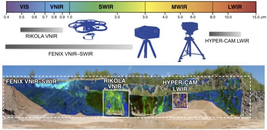
- While the potential of combining VNIR, SWIR and LWIR hyperspectral data for geological mapping has been recognized [12,38,39,40], hyperspectral imagers have been operated from a single platform, usually airborne (e.g., [41,42]). Recently, the Helmholtz Institute Freiberg for Resource Technology started to deploy hyperspectral sensors on the ground [24,37], and on unmanned aerial systems [43,44]. This approach allows for higher spatial resolutions (from millimeters to tens of centimeters) and a range of scanning perspectives, which can be advantageous, particularly in areas with steep outcrops and poorly accessible and potentially dangerous terrain.
- Digital outcrop models are traditionally based on data obtained from laser scanning (e.g., [4,45,46,47]) or photogrammetric techniques (e.g., [48,49,50,51,52]). Fusion between hyperspectral and 3D outcrop data is mostly based on terrestrial laser scanning (TLS) data (e.g., [20,21,22,23,53,54]). TLS can be used to derive highly precise outcrop models (e.g., [48,55,56,57]), but these are prone to containing data gaps caused by occlusion, particular in areas of high relief. The effect of occlusion can be reduced by obtaining TLS data from multiple scan locations, but this is time-consuming, and can be impeded in areas of restricted accessibility. Airborne laser scanning may supplement TLS, but it requires substantial financial and logistical efforts. Alternatively, 3D outcrop geometry may be reconstructed rapidly, safely, and cost-efficiently by the means of Structure-from-Motion Multi-View Stereo (SfM-MVS, or simply SfM) photogrammetry. Due to the varying image acquisition angles, SfM point clouds based on terrestrial and aerial photographs are less influenced by occlusion, and they can serve as a basis for the fusion of spectral datasets with varied sensor positions.
2. Case Study
3. Methods and Materials
3.1. Ground-Based VNIR–SWIR Hyperspectral Imaging
- Conversion to at-sensor radiance: The first step included dark-current subtraction, followed by image normalization and multiplication of the sensor- and band-specific radiometric calibration data.
- Optical distortion correction: In this step, sensor-specific optical distortions were corrected for. In case of the Specim AisaFenix scanner, this encompassed fish-eye- and slit-bending effects, which could be removed by applying sensor-specific correction values for each pixel in the field of view (FOV).
- Conversion to at-sensor reflectance: This conversion was achieved by an empirical line calibration using a white reference panel (Spectralon SRS-99, [71]) placed in the scene with a similar orientation to the target.
- Orthorectification and georeferencing: A corresponding photogrammetric point cloud (see below) was transformed, projected, and rasterized to represent the viewing angle of the hyperspectral sensor. In case of data acquired with the Specim AisaFenix, a cylindrical projection was used to account for the panoramic imaging geometry of push broom scanners (see [24] for details). The resulting acquisition-specific pseudo-orthophoto contained red-green-blue (RGB) values, original coordination, and sun incidence angles for each rasterized pixel. Subsequently, the hyperspectral image was referenced to the pseudo-orthophoto based on 23 manual tie points that were spread evenly over the entire scene.
- Conversion to at-target reflectance: The hyperspectral image may be influenced by illumination differences due to topography. These were corrected for by c-factor topographic correction (see [43] for details) based on pixel-specific sun incidence angles, which were determined for each point of the photogrammetric 3D point cloud and stored in each pixel of the created pseudo-orthophoto, as described above.
3.2. Ground-Based LWIR Hyperspectral Imaging
- Conversion to radiance: Immediately after acquisition, the raw interferometer data frame was automatically converted to radiance based on the offset and gain of an internal blackbody calibration. For internal calibration, the device features two blackbodies, the temperatures of which were adjusted to bracket the expected temperature range of the measured scenario to minimize the non-linearity effects of the instrument’s response.
- Temperature-emissivity separation: To achieve the radiometric calibration, a temperature-emissivity separation (TES) was performed using the algorithms of the TES-MATLAB toolbox developed by Telops. A custom-made diffuse reflector (brushed Al-panel, Al 6082 alloy) and a blackbody (Al panel, milled and sprayed with black Würth acrylic lacquer paint) were placed in the scene during acquisition. Whereas the diffuse reflector (high reflectivity, low emissivity) was used to estimate the atmospheric downwelling radiance, the blackbody (high emissivity, low reflectivity) was used to determine the emissivity of the target, which varies according to the temperature-specific Planck function and the atmospheric transmittance between the sensor and target. Other parameters needed for the TES were the emissivities of both reference surfaces (in the Naundorf LWIR scene 0.95 and 0.17, for the blackbody and the reflector, respectively), the panel temperatures, which for the Naundorf LWIR scene were extracted from the brightness–temperature image (blackbody 51.78 °C; diffuse reflector 21.35 °C, measured at the water vapor line at 282.15 K), and the ambient air temperature (26.7 °C, measured with a digital thermometer). The TES returns both a temperature image and the spectral emissivity data cube.
- Image stitching: In order to stitch the individual image frames together to a mosaic, the automatic key point detection and matching workflow from [43] was successfully adapted to the LWIR data. The data cubes were automatically matched using a looping trial-and-error procedure, which eliminated the need for prior image sorting. The created mosaic was subsequently orthorectified and referenced to a scene-specific pseudo-orthophoto using 22 manually collected tie points.
3.3. Drone-Borne VNIR Hyperspectral Imaging
- Conversion to radiance: First, a dark current subtraction was performed on the individual images and the raw digital numbers were converted to radiance with the software provided by Senop.
- Lens correction and co-registration: Specific lens distortions caused by internal camera features were corrected for with the MEPHySTo toolbox. Moreover, spatial shifts between the single bands occurred during image capture, due to sensor movement. Therefore, the spectral bands were co-registered with one another using the toolbox.
- Orthorectification and georeferencing: Subsequently, the toolbox was used to automatically orthorectify and georeference the images. This was done through keypoint detection and point-matching algorithms to match points between the hyperspectral images and a view-specific pseudo-orthophoto generated from an SfM point cloud.
- Topographic correction: The topography of the area, such as various orientated slopes, can influence the illumination within an image. The radiance of the same material can vary, due to different sunlight incidences on that material. The MEPHySTo toolbox was used to perform these topographic corrections.
- Mosaicking: The orthorectified and georeferenced images were then simply merged together using the toolbox, to create a mosaic of the whole area.
- Atmospheric correction: Finally, the hyperspectral radiance mosaic was converted to reflectance. An empirical line method was used by using known spectra from black, white, and grey Polyvinyl chloride (PVC) panels placed in the scene.
3.4. Photogrammetry and 3D Integration
3.5. XRD and Spectrometric Analysis
4. Results: Case Study Naundorf Quarry (Germany)
4.1. Validation Data
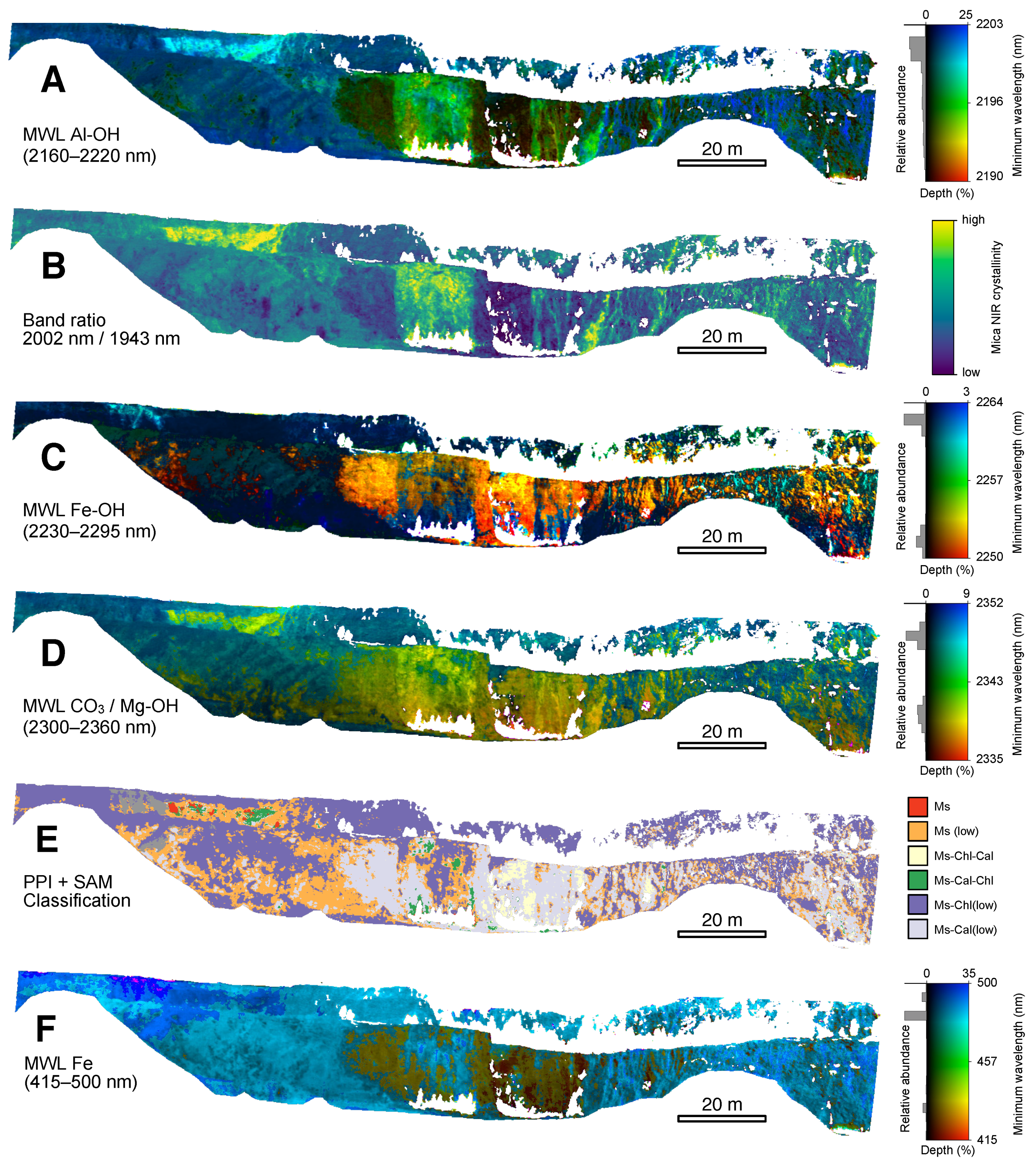
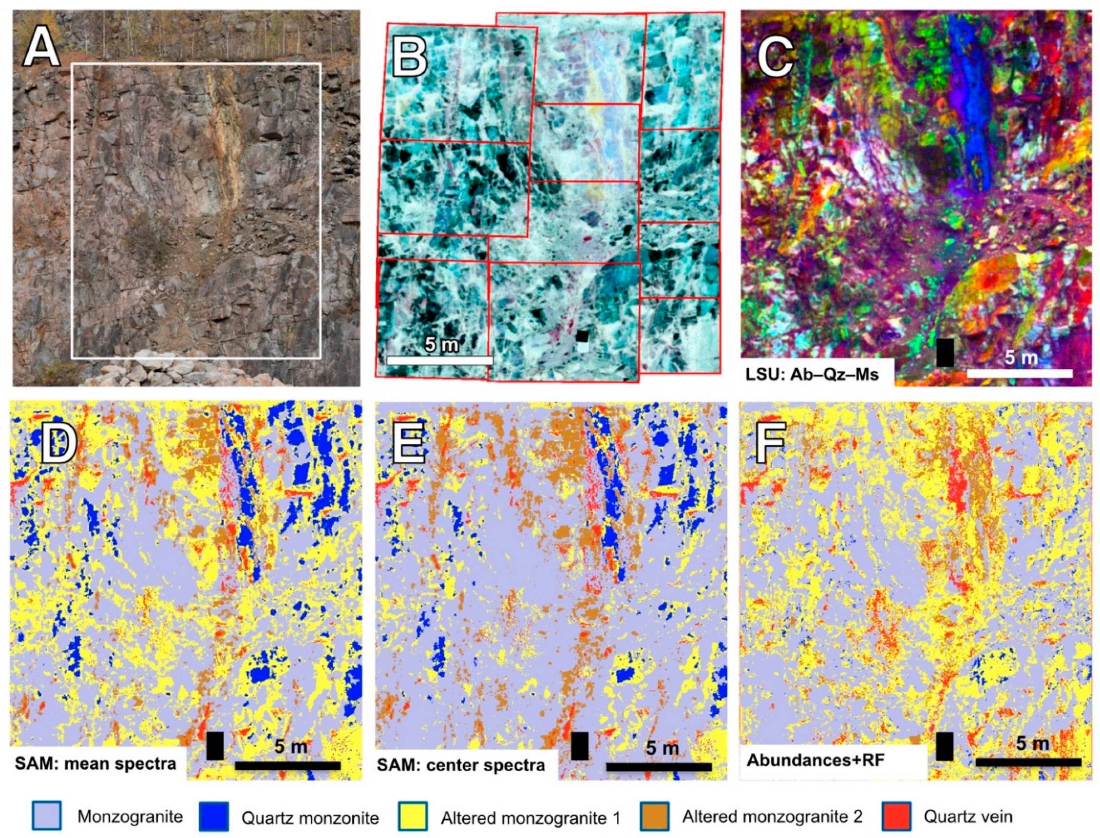
4.2. Ground-Based VNIR–SWIR Hyperspectral Imaging
4.3. Ground-Based LWIR Hyperspectral Imaging
4.4. UAV-Based VNIR Hyperspectral Imaging
4.5. SfM Photogrammetry
4.6. 3D Integration
5. Discussion
5.1. Quarry Naundorf
5.2. Benefits of the Integrated Workflow
6. Conclusions
- spectral range, as the combination of visible to near infrared, shortwave infrared, and long-wave infrared hyperspectral imaging enables the discrimination of a variety of geologic materials such as rock-forming and hydrothermal alteration minerals;
- spatial coverage, as the combined use of ground-based sensors and unmanned aerial vehicles (UAV) allows for close-range imagery with higher spatial resolutions to be acquired of geological outcrops from a number of perspectives;
- flexibility, as SfM outcrop models based on terrestrial and aerial photographs are less influenced by occlusion, and can serve as a basis for fusion of multiple spectral datasets with different sensor positions;
- validation, as geological field observations and analytical validation data are supplemented by a range of cross-validation data between the individual datasets of the multi-sensor approach;
- cost- and time-efficiency, as the SfM approach offers a fast and low-cost alternative to terrestrial laser scanning and the presented hyperspectral processing routine, which is mostly based on open source code, requires only minimal user input;
- geological interpretation, as the hypercloud, i.e., a geometrically correct, spatially 3-dimensional representation of the hyperspectral data cube or its derivatives, allows for an intuitive visualization of geological outcrops, and it can be used to identify and extract geologic structures as well as map areal distributions of lithologic domains.
Author Contributions
Funding
Acknowledgments
Conflicts of Interest
References
- Hodgetts, D.; Drinkwater, N.J.; Hodgson, J.; Kavanagh, J.; Flint, S.S.; Keogh, K.J.; Howell, J.A. Three-dimensional geological models from outcrop data using digital data collection techniques: An example from the Tanqua Karoo depocentre, South Africa. GSL Spec. Pub. 2004, 239, 57–75. [Google Scholar] [CrossRef]
- Enge, H.D.; Buckley, S.J.; Rotevatn, A.; Howell, J.A. From outcrop to reservoir simulation model: Workflow and procedures. Geosphere 2007, 3, 469–490. [Google Scholar] [CrossRef]
- Rotevatn, A.; Buckley, S.J.; Howell, J.A.; Fossen, H. Overlapping faults and their effect on fluid flow in different reservoir types: A LIDAR-based outcrop modeling and flow simulation study. AAPG Bull. 2009, 93, 407–427. [Google Scholar] [CrossRef]
- Buckley, S.J.; Enge, H.D.; Carlsson, C.; Howell, J.A. Terrestrial laser scanning for use in virtual outcrop geology. Photogramm. Rec. 2010, 25, 225–239. [Google Scholar] [CrossRef] [Green Version]
- Rarity, F.; van Lanen, X.M.T.; Hodgetts, D.; Gawthorpe, R.L.; Wilson, P.; Fabuel-Perez, I.; Redfern, J. LiDAR-based digital outcrops for sedimentological analysis: Workflows and techniques. GSL Spec. Pub. 2014, 387, 153–183. [Google Scholar] [CrossRef]
- Goetz, A.F.H.; Vane, G.; Solomon, J.E.; Rock, B.N. Imaging Spectrometry for Earth Remote-Sensing. Science 1985, 228, 1147–1153. [Google Scholar] [CrossRef] [PubMed]
- Goetz, A.F.H. Three decades of hyperspectral remote sensing of the Earth: A personal view. Remote Sens. Environ. 2009, 113, S5–S16. [Google Scholar] [CrossRef]
- Kruse, F.A. Use of Airborne Imaging Spectrometer Data to Map Minerals Associated with Hydrothermally Altered Rocks in the Northern Grapevine Mountains, Nevada, and California. Remote Sens. Environ. 1988, 24, 31–51. [Google Scholar] [CrossRef]
- Kirkland, L.; Herr, K.; Keim, E.; Adams, P.; Salisbury, J.; Hackwell, J.; Treiman, A. First use of an airborne thermal infrared hyperspectral scanner for compositional mapping. Remote Sens. Environ. 2002, 80, 447–459. [Google Scholar] [CrossRef] [Green Version]
- Jones, S.; Herrmann, W.; Gemmell, J.B. Short Wavelength Infrared Spectral Characteristics of the HW Horizon: Implications for Exploration in the Myra Falls Volcanic-Hosted Massive Sulfide Camp, Vancouver Island, British Columbia, Canada. Econ. Geol. 2005, 100, 273–294. [Google Scholar] [CrossRef]
- Van der Meer, F.D.; van der Werff, H.M.A.; van Ruitenbeek, F.J.A.; Hecker, C.A.; Bakker, W.H.; Noomen, M.F.; van der Meijde, M.; Carranza, E.J.M.; de Smeth, J.B.; Woldai, T. Multi- and hyperspectral geologic remote sensing: A review. Int. J. Appl. Earth Obs. Geoinf. 2012, 14, 112–128. [Google Scholar] [CrossRef]
- Kruse, F.A. Integrated visible and near-infrared, shortwave infrared, and longwave infrared full-range hyperspectral data analysis for geologic mapping. J. Appl. Remote Sens. 2015, 9, 096005. [Google Scholar] [CrossRef] [Green Version]
- Hunt, G.R. Spectral signatures of particulate minerals in the visible and near infrared. Geophysics 1977, 42, 501–513. [Google Scholar] [CrossRef] [Green Version]
- Hunt, G.R. Near-infrared (1.3-2.4) μm spectra of alteration minerals-Potential for use in remote sensing. Geophysics 1979, 44, 1974–1986. [Google Scholar] [CrossRef]
- Clark, R.N.; King, T.V.V.; Klejwa, M.; Swayze, G.A.; Vergo, N. High spectral resolution reflectance spectroscopy of minerals. J. Geophys. Res. 1990, 95, 12653–12680. [Google Scholar] [CrossRef]
- Salisbury, J.W.; Walter, L.S.; Vergo, N.; D’Aria, D.M. Infrared (2.1–2.5 µm) Spectra of Minerals; John Hopkins University Press: Baltimore, MD, USA, 1991. [Google Scholar]
- Baldridge, A.M.; Hook, S.J.; Grove, C.I.; Rivera, G. The ASTER spectral library version 2.0. Remote Sens. Environ. 2009, 113, 711–715. [Google Scholar] [CrossRef]
- Laukamp, C. Short Wave Infrared Functional Groups of Rock-Forming Minerals; CSIRO, Report number EP115222; CSIRO: Canberra, Australia, 2011; pp. 1–20. [Google Scholar]
- Kokaly, R.F.; Clark, R.N.; Swayze, G.A.; Livo, K.E.; Hoefen, T.M.; Pearson, N.C.; Wise, R.A.; Benzel, W.M.; Lowers, H.A.; Driscoll, R.L.; et al. USGS Spectral Library Version 7; U.S. Geological Survey Data Series; United States Geological Survey: Reston, VA, USA, 2017; Volume 1035, 61p. [CrossRef]
- Kurz, T.H.; Buckley, S.J.; Howell, J.A.; Schneider, D. Integration of panoramic hyperspectral imaging with terrestrial lidar data. Photogramm. Rec. 2011, 26, 212–228. [Google Scholar] [CrossRef]
- Kurz, T.H.; Buckley, S.J.; Howell, J.A. Close-range hyperspectral imaging for geological field studies: Workflow and methods. Int. J. Remote Sens. 2013, 34, 1798–1822. [Google Scholar] [CrossRef]
- Buckley, S.J.; Kurz, T.H.; Howell, J.A.; Schneider, D. Terrestrial lidar and hyperspectral data fusion products for geological outcrop analysis. Comput. Geosci. 2013, 54, 249–258. [Google Scholar] [CrossRef]
- Kurz, T.H.; Buckley, S.J. A review of hyperspectral imaging in close range applications. Int. Arch. Photogramm. Remote Sens. Spat. Inf. Sci. 2016, XLI-B5, 865–870. [Google Scholar] [CrossRef]
- Lorenz, S.; Salehi, S.; Kirsch, M.; Zimmermann, R.; Unger, G.; Vest Sørensen, E.; Gloaguen, R. Radiometric Correction and 3D Integration of Long-Range Ground-Based Hyperspectral Imagery for Mineral Exploration of Vertical Outcrops. Remote Sens. 2018, 10, 176. [Google Scholar] [CrossRef]
- Salehi, S.; Lorenz, S.; Vest Sørensen, E.; Zimmermann, R.; Fensholt, R.; Henning Heincke, B.; Kirsch, M.; Gloaguen, R. Integration of Vessel-Based Hyperspectral Scanning and 3D-Photogrammetry for Mobile Mapping of Steep Coastal Cliffs in the Arctic. Remote Sens. 2018, 10, 175. [Google Scholar] [CrossRef]
- Hunt, G.J.; Salisbury, J.W. Visible and Near-Infrared Spectra of Minerals and Rocks. I. Silicate Minerals. Mod. Geol. 1970, 1, 283–300. [Google Scholar]
- Salisbury, J.W.; D’Aria, D.M. Emissivity of terrestrial materials in the 8–14 μm atmospheric window. Remote Sens. Environ. 1992, 42, 83–106. [Google Scholar] [CrossRef]
- Hecker, C.; van der Meijde, M.; van der Meer, F.D. Thermal infrared spectroscopy on feldspars—Successes, limitations and their implications for remote sensing. ESR 2010, 103, 60–70. [Google Scholar] [CrossRef]
- Hecker, C.; Hook, S.; Meijde, M.V.D.; Bakker, W.; Werff, H.V.D.; Wilbrink, H.; Ruitenbeek, F.V.; de Smeth, B.; Meer, F.V.D. Thermal Infrared Spectrometer for Earth Science Remote Sensing Applications—Instrument Modifications and Measurement Procedures. Sensors 2011, 11, 10981–10999. [Google Scholar] [CrossRef] [PubMed] [Green Version]
- Hecker, C.; Dilles, J.H.; van der Meijde, M.; van der Meer, F.D. Thermal infrared spectroscopy and partial least squares regression to determine mineral modes of granitoid rocks. Geochem. Geophys. Geosyst. 2012, 13, Q03021. [Google Scholar] [CrossRef]
- Eisele, A.; Chabrillat, S.; Hecker, C.; Hewson, R.; Lau, I.C.; Rogass, C.; Segl, K.; Cudahy, T.J.; Udelhoven, T.; Hostert, P.; et al. Advantages using the thermal infrared (TIR) to detect and quantify semi-arid soil properties. Remote Sens. Environ. 2015, 163, 296–311. [Google Scholar] [CrossRef]
- Green, D.; Schodlok, M.; Green, D.; Schodlok, M. Characterisation of carbonate minerals from hyperspectral TIR scanning using features at 14 000 and 11 300 nm. Aust. J. Earth Sci. 2016, 1–8. [Google Scholar] [CrossRef]
- Vaughan, R.G.; Calvin, W.M.; Taranik, J.V. SEBASS hyperspectral thermal infrared data: Surface emissivity measurement and mineral mapping. Remote Sens. Environ. 2003, 85, 48–63. [Google Scholar] [CrossRef]
- Riley, D.N.; Hecker, C.A. Mineral Mapping with Airborne Hyperspectral Thermal Infrared Remote Sensing at Cuprite, Nevada, USA. In Thermal Infrared Remote Sensing; Remote Sensing and Digital Image Processing; Springer: Dordrecht, The Netherlands, 2013; Volume 17, pp. 495–514. [Google Scholar] [CrossRef]
- Weksler, S.; Notesco, G.; Ben-Dor, E. An automated procedure for reducing atmospheric features and emphasizing surface emissivity in hyperspectral longwave infrared (LWIR) images. Int. J. Remote Sens. 2017, 38, 4481–4493. [Google Scholar] [CrossRef]
- Vitins, I.; Felix, H.; Eisele, A.; Hueni, A.; Hewson, R.D. Pit-wall face mapping of carbonate mixtures using LWIR remote sensing. In Proceedings of the 10th EARSeL SIG Imaging Spectroscopy Workshop, University of Zurich, Zurich, Switzerland, 19–21 April 2017. [Google Scholar]
- Kirsch, M.; Lorenz, S.; Zimmermann, R.; Möckel, R.; Khodadadzadeh, M.; Tusa, L.; Chamberland, M.; Gloaguen, R. Terrestrial long-wave infrared hyperspectral imaging for geological mapping: A case study. Geophys. Res. Abstr. 2018, 20, EGU2018-10262. [Google Scholar]
- McDowell, M.; Kruse, F.A. Enhanced Compositional Mapping through Integrated Full-Range Spectral Analysis. Remote Sens. 2016, 8, 757. [Google Scholar] [CrossRef]
- Notesco, G.; Kopačková, V.; Rojík, P.; Schwartz, G.; Livne, I.; Dor, E. Mineral Classification of Land Surface Using Multispectral LWIR and Hyperspectral SWIR Remote-Sensing Data. A Case Study over the Sokolov Lignite Open-Pit Mines, the Czech Republic. Remote Sens. 2014, 6, 7005–7025. [Google Scholar] [CrossRef] [Green Version]
- Notesco, G.; Ogen, Y.; Ben-Dor, E. Integration of Hyperspectral Shortwave and Longwave Infrared Remote-Sensing Data for Mineral Mapping of Makhtesh Ramon in Israel. Remote Sens. 2016, 8, 318. [Google Scholar] [CrossRef]
- Harris, J.R.; Rogge, D.; Hitchcock, R.; Ijewliw, O.; Wright, D. Mapping lithology in Canada’s Arctic: Application of hyperspectral data using the minimum noise fraction transformation and matched filtering. Can. J. Earth Sci. 2005, 42, 2173–2193. [Google Scholar] [CrossRef]
- Bellian, J.A.; Beck, R.; Kerans, C. Analysis of hyperspectral and lidar data: Remote optical mineralogy and fracture identification. Geosphere 2007, 3, 491–500. [Google Scholar] [CrossRef]
- Jakob, S.; Zimmermann, R.; Gloaguen, R. The Need for Accurate Geometric and Radiometric Corrections of Drone-Borne Hyperspectral Data for Mineral Exploration: MEPHySTo—A Toolbox for Pre-Processing Drone-Borne Hyperspectral Data. Remote Sens. 2017, 9, 88. [Google Scholar] [CrossRef]
- Jackisch, R.; Lorenz, S.; Zimmermann, R.; Möckel, R.; Gloaguen, R. Drone-Borne Hyperspectral Monitoring of Acid Mine Drainage: An Example from the Sokolov Lignite District. Remote Sens. 2018, 10, 385. [Google Scholar] [CrossRef]
- Bellian, J.A.; Kerans, C.; Jennette, D.C. Digital Outcrop Models: Applications of Terrestrial Scanning Lidar Technology in Stratigraphic Modeling. JSR 2005, 75, 166–176. [Google Scholar] [CrossRef] [Green Version]
- Buckley, S.J.; Howell, J.A.; Enge, H.D.; Kurz, T.H. Terrestrial laser scanning in geology: Data acquisition, processing and accuracy considerations. J. Geol. Soc. Lond. 2008, 165, 625–638. [Google Scholar] [CrossRef]
- Heritage, G.L.; Large, A.R.G. Laser Scanning for the Environmental Sciences; Heritage, G.L., Large, A.R.G., Eds.; Wiley-Blackwell: Oxford, UK, 2009. [Google Scholar]
- James, M.R.; Robson, S. Straightforward reconstruction of 3D surfaces and topography with a camera: Accuracy and geoscience application. J. Geophys. Res. Earth Surf. 2012, 117, F03017. [Google Scholar] [CrossRef]
- James, M.R.; Robson, S. Mitigating systematic error in topographic models derived from UAV and ground-based image networks. Earth Surf. Process. Landf. 2014, 39, 1413–1420. [Google Scholar] [CrossRef] [Green Version]
- Westoby, M.J.; Brasington, J.; Glasser, N.F.; Hambrey, M.J.; Reynolds, J.M. “Structure-from-Motion” photogrammetry: A low-cost, effective tool for geoscience applications. Geomorphology 2012, 179, 300–314. [Google Scholar] [CrossRef] [Green Version]
- Bemis, S.P.; Micklethwaite, S.; Turner, D.; James, M.R.; Akciz, S.; Thiele, S.T.; Bangash, H.A. Ground-based and UAV-Based photogrammetry: A multi-scale, high- resolution mapping tool for structural geology and paleoseismology. J. Struct. Geol. 2014, 69, 163–178. [Google Scholar] [CrossRef]
- Eltner, A.; Kaiser, A.; Castillo, C.; Rock, G.; Neugirg, F.; Abellán, A. Image-based surface reconstruction in geomorphometry—Merits, limits and developments of a promising tool for geoscientists. Earth Surf. Dynam. Discuss. 2015, 3, 1445–1508. [Google Scholar] [CrossRef]
- Murphy, R.J.; Monteiro, S.T.; Schneider, S. Evaluating Classification Techniques for Mapping Vertical Geology Using Field-Based Hyperspectral Sensors. IEEE Trans. Geosci. Remote Sens. 2012, 50, 3066–3080. [Google Scholar] [CrossRef]
- Murphy, R.J.; Monteiro, S.T. Mapping the distribution of ferric iron minerals on a vertical mine face using derivative analysis of hyperspectral imagery (430–970nm). ISPRS J. Photogramm. Remote Sens. 2013, 75, 29–39. [Google Scholar] [CrossRef]
- Wilkinson, M.W.; Jones, R.R.; Woods, C.E.; Gilment, S.R.; McCaffrey, K.J.W.; Kokkalas, S.; Long, J.J. A comparison of terrestrial laser scanning and structure-from-motion photogrammetry as methods for digital outcrop acquisition. Geosphere 2016, 12, 1865–1880. [Google Scholar] [CrossRef] [Green Version]
- Cawood, A.J.; Bond, C.E.; Howell, J.A.; Butler, R.W.H.; Totake, Y. LiDAR, UAV or compass-clinometer? Accuracy, coverage and the effects on structural models. J. Struct. Geol. 2017, 98, 67–82. [Google Scholar] [CrossRef] [Green Version]
- James, M.R.; Robson, S.; d’Oleire-Oltmanns, S.; Niethammer, U. Optimising UAV topographic surveys processed with structure-from-motion: Ground control quality, quantity and bundle adjustment. Geomorphology 2017, 280, 51–66. [Google Scholar] [CrossRef]
- Kruse, F.A.; Bedell, R.L.; Taranik, J.V.; Peppin, W.A.; Weatherbee, O.; Calvin, W.M. Mapping alteration minerals at prospect, outcrop and drill core scales using imaging spectrometry. Int. J. Remote Sens. 2012, 33, 1780–1798. [Google Scholar] [CrossRef] [PubMed]
- Spinetti, C.; Mazzarini, F.; Casacchia, R.; Colini, L.; Neri, M.; Behncke, B.; Salvatori, R.; Buongiorno, M.F.; Pareschi, M.T. Spectral properties of volcanic materials from hyperspectral field and satellite data compared with LiDAR data at Mt. Etna. Int. J. Appl. Earth Obs. Geoinf. 2009, 11, 142–155. [Google Scholar] [CrossRef]
- Kereszturi, G.; Schaefer, L.N.; Schleiffarth, W.K.; Procter, J.; Pullanagari, R.R.; Mead, S.; Kennedy, B. Integrating airborne hyperspectral imagery and LiDAR for volcano mapping and monitoring through image classification. Int. J. Appl. Earth Obs. Geoinf. 2018, 73, 323–339. [Google Scholar] [CrossRef]
- Van der Meer, F.; Kopačková, V.; Koucká, L.; van der Werff, H.M.A.; van Ruitenbeek, F.J.A.; Bakker, W.H. Wavelength feature mapping as a proxy to mineral chemistry for investigating geologic systems: An example from the Rodalquilar epithermal system. Int. J. Appl. Earth Obs. Geoinf. 2018, 64, 237–248. [Google Scholar] [CrossRef]
- Murphy, R.J.; Taylor, Z.; Schneider, S.; Nieto, J. Mapping clay minerals in an open-pit mine using hyperspectral and LiDAR data. Eur. J. Remote Sens. 2015, 48, 511–526. [Google Scholar] [CrossRef] [Green Version]
- Kroner, U.; Romer, R.L. Two plates—Many subduction zones: The Variscan orogeny reconsidered. Gondwana Res. 2013, 24, 298–329. [Google Scholar] [CrossRef]
- Tichomirowa, M. 207Pb/206Pb-Einzelzirkondatierungen zur Bestimmung des Intrusionsalters des Niederbobritzscher Granites. Terra Nostra 1997, 8, 183–184. [Google Scholar]
- Förster, H.-J.; Tischendorf, G.; Trumbull, R.B.; Gottesmann, B. Late-Collisional Granites in the Variscan Erzgebirge, Germany. J. Pet. 1999, 40, 1613–1645. [Google Scholar] [CrossRef]
- Müller, H. Die Erzgänge des Freiberger Bergrevieres—Erläuterungen zur geololgischen Specialkarte des Königreichs Sachsen; Königliches Finanzministerium: Leipzig, Germany, 1901; 366p. [Google Scholar]
- Rösler, H.J.; Pilot, J.; Starke, R.; Schreiter, E. Die Vererzungen im Granit von Niederbobritzsch bei Freiberg. Abh. Staatl. Mus. Miner. Geol. Dresd. 1990, 37, 103–123. [Google Scholar]
- Seifert, T.; Sandmann, D. Mineralogy and geochemistry of indium-bearing polymetallic vein-type deposits: Implications for host minerals from the Freiberg district, Eastern Erzgebirge, Germany. Ore Geol. Rev. 2006, 28, 1–31. [Google Scholar] [CrossRef]
- Kamb, W.B. Ice Petrofabric Observations from Blue Glacier, Washington, in Relation to Theory and Experiment. J. Geophys. Res. 1959, 64, 1891–1909. [Google Scholar] [CrossRef]
- AisaFENIX Hyperspectral Sensor. 2018. Available online: http://www.specim.fi/products/aisafenix-hyperspectral-sensor/ (accessed on 18 August 2018).
- Spectralon Technical Datashet-Reflectance Materials and Coatings; Technical Guide; Labsphere: North Sutton, NH, USA, 2016; pp. 1–26.
- Green, A.A.; Berman, M.; Switzer, P.; Craig, M.D. A Transformation for Ordering Multispectral Data in Terms of Image Quality with Implications for Noise Removal. IEEE Trans. Geosci. Remote Sens. 1988, 26, 65–74. [Google Scholar] [CrossRef]
- Pontual, S.; Merry, N.; Gamson, P. Spectral Analysis Guides for Mineral Exploration; AusSpec International Pty.: Arrowtown, New Zealand, 1997; Volumes 1–7. [Google Scholar]
- Crowley, J.K.; Williams, D.E.; Hammarstrom, J.M.; Piatak, N.; Chou, I.-M.; Mars, J.C. Spectral reflectance properties (0.4–2.5 μm) of secondary Fe-oxide, Fe-hydroxide, and Fe-sulphate-hydrate minerals associated with sulphide-bearing mine wastes. Geochem. Explor. Environ. Anal. 2003, 3, 219–228. [Google Scholar] [CrossRef]
- Bakker, W.H.; van Ruitenbeek, F.J.A.; van der Werff, H.M.A.; Zegers, T.E.; Oosthoek, J.H.P.; Marsh, S.H.; van der Meer, F.D. Processing OMEGA/Mars Express hyperspectral imagery from radiance-at-sensor to surface reflectance. Planet. Space Sci. 2014, 90, 1–9. [Google Scholar] [CrossRef]
- Van der Meer, F. Analysis of spectral absorption features in hyperspectral imagery. Int. J. Appl. Earth Obs. Geoinf. 2004, 5, 55–68. [Google Scholar] [CrossRef]
- Boardman, J.W.; Kruse, F.A.; Green, R.O. Mapping target signatures via partial unmixing of AVIRIS data. In Proceedings of the Fifth JPL Airborne Earth Science Workshop, Pasadena, CA, USA, 23–26 January 1995; pp. 95–101. [Google Scholar]
- Heylen, R.; Scheunders, P. Multidimensional Pixel Purity Index for Convex Hull Estimation and Endmember Extraction. IEEE Trans. Geosci. Remote Sens. 2013, 51, 4059–4069. [Google Scholar] [CrossRef]
- Winter, M.E. N-FINDR: An algorithm for fast autonomous spectral end-member determination in hyperspectral data. In Proceedings of SPIE—The International Society for Optical Engineering; Descour, M.R., Shen, S.S., Eds.; University of Queensland: Brisbane, Australia, 1999; Volume 3753, pp. 266–275. [Google Scholar]
- Kruse, F.A.; Lefkoff, A.B.; Boardman, J.W.; Heidebrecht, K.B.; Shapiro, A.T.; Barloon, P.J.; Goetz, A.F.H. The spectral image processing system (SIPS)—Interactive visualization and analysis of imaging spectrometer data. Remote Sens. Environ. 1993, 44, 145–163. [Google Scholar] [CrossRef]
- Telops Hyperspectral IR Cameras. 2018. Available online: http://telops.com/products/hyperspectral-cameras (accessed on 18 August 2018).
- Schlerf, M.; Rock, G.; Lagueux, P.; Ronellenfitsch, F.; Gerhards, M.; Hoffmann, L.; Udelhoven, T. A Hyperspectral Thermal Infrared Imaging Instrument for Natural Resources Applications. Remote Sens. 2012, 4, 3995–4009. [Google Scholar] [CrossRef] [Green Version]
- Boardman, J.W. Sedimentary Facies Analysis Using Imaging Spectrometry: A Geophysical Inverse Problem. Ph.D. Thesis, University of Colorado, Boulder, CO, USA, 1991. [Google Scholar]
- Adams, J.B.; Smith, M.O.; Gillespie, A.R. Imaging spectroscopy: Interpretation based on spectral mixture analysis. In Remote Geochemical Analysis Elemental and Mineralogical Composition; Pieters, C.M., Englert, P.A., Eds.; Cambridge Univ. Press: Cambridge, UK, 1993; pp. 145–166. ISBN 9780521402811. [Google Scholar]
- Li, H.C.; Chang, C.I. Linear spectral unmixing using least squares error, orthogonal projection and simplex volume for hyperspectral images. In Proceedings of the 7th Workshop on Hyperspectral Image and Signal Processing: Evolution in Remote Sensing (WHISPERS), Tokyo, Japan, 2–5 June 2015; pp. 1–4. [Google Scholar]
- Liaw, A.; Wiener, M. Classification and Regression by randomForest. R News 2002, 2, 18–22. [Google Scholar]
- Silván-Cárdenas, J.L.; Wang, L. Fully Constrained Linear Spectral Unmixing: Analytic Solution Using Fuzzy Sets. IEEE Trans. Geosci. Remote Sens. 2010, 48, 3992–4002. [Google Scholar] [CrossRef]
- Optronics Hyperspectral—The RIKOLA Product Range. 2018. Available online: http://senop.fi/en/optronics-hyperspectral (accessed on 18 August 2018).
- Aibot X6—Robust and Reliable UAV Solution. 2018. Available online: https://leica-geosystems.com/en-gb/products/uav-systems/aibot-x6 (accessed on 18 August 2018).
- Savitzky, A.; Golay, M.J.E. Smoothing and Differentiation of Data by Simplified Least Squares Procedures. Anal. Chem. 1964, 36, 1627–1639. [Google Scholar] [CrossRef]
- Sensefly eBee Classic. 2018. Available online: https://www.sensefly.com/drone/ebee-mapping-drone/ (accessed on 18 August 2018).
- Carrivick, J.L.; Smith, M.W.; Quincey, D.J. Structure from Motion in the Geosciences; Wiley-Blackwell: Hoboken, NJ, USA, 2016; ISBN 9781118895849. [Google Scholar]
- Doebelin, N.; Kleeberg, R. IUCr Profex: A graphical user interface for the Rietveld refinement program BGMN. J. Appl. Crystallogr. 2015, 48, 1573–1580. [Google Scholar] [CrossRef] [PubMed]
- Vernon, R.H. Crystallization and hybridism in microgranitoid enclave magmas: Microstructural evidence. J. Geophys. Res. Solid Earth 1990, 95, 17849–17859. [Google Scholar] [CrossRef]
- Hibbard, M.J. Textural anatomy of twelve magma-mixed granitoid systems. In Enclaves and Granite Petrology, Developments in Petrology 13; Didier, J., Barbarin, B., Eds.; Elsevier Science: Amsterdam, The Netherlands, 1991; pp. 431–444. [Google Scholar]
- Rösler, H.J.; Bothe, M. Bemerkungen zur Petrologie des Granites von Niederbobritzsch bei Freiberg und zur Bildung der Allanite. Abh. Staat. Mus. Mineral. Geol. Dresd. 1990, 37, 73–101. [Google Scholar]
- Rösler, H.J.; Budzinski, H. Das Bauprinzip des Granits von Niederbobritzsch bei Freiberg/Sa. auf Grund seiner geochemischen Analyse. Z. Geol. Wiss. 1994, 22, 307–324. [Google Scholar]
- Whitney, D.L.; Evans, B.W. Abbreviations for names of rock-forming minerals. Am. Miner. 2010, 95, 185–187. [Google Scholar] [CrossRef]
- Post, J.L.; Noble, P.N. The Near-Infrared Combination Band Frequencies of Dioctahedral Smectites, Micas, and Illites. Clays Clay Miner. 1993, 41, 639–644. [Google Scholar] [CrossRef]
- Herrmann, W.; Blake, M.; Doyle, M.; Huston, D.; Kamprad, J.; Merry, N.; Pontual, S. Short Wavelength Infrared (SWIR) Spectral Analysis of Hydrothermal Alteration Zones Associated with Base Metal Sulfide Depositsat Rosebery and Western Tharsis, Tasmania, and Highway-Reward, Queensland. Econ. Geol. 2001, 96, 939–955. [Google Scholar] [CrossRef]
- Dalm, M.; Buxton, M.W.N.; van Ruitenbeek, F.J.A.; Voncken, J.H.L. Application of near-infrared spectroscopy to sensor based sorting of a porphyry copper ore. Miner. Eng. 2014, 58, 7–16. [Google Scholar] [CrossRef]
- Yang, K.; Huntington, J.F.; Scott, K.M.; Mason, P. Alteration Zoning in the Volcanic Rocks at Hishikari, Japan, as Revealed by Short Wavelength Infrared Spectroscopy; Exploration and Mining Report 203R, CSIRO/AMIRA Project P435—Mineral Mapping with Field Spectroscopy for Exploration; CSIRO Division of Exploration and Mining, Institute of Minerals, Energy and Construction: Canberra, Australia, 1996. [Google Scholar]
- Scott, K.M.; Yang, K. Spectral Reflectance Studies of White Micas; Exploration and Mining Report 439R, CSIRO/AMIRA Project P435—Mineral Mapping with Field Spectroscopy for Exploration; CSIRO Division of Exploration and Mining, Institute of Minerals, Energy and Construction: Canberra, Australia, 1997. [Google Scholar]
- Fukuchi, R.; Fujimoto, K.; Kameda, J.; Hamahashi, M.; Yamaguchi, A.; Kimura, G.; Hamada, Y.; Hashimoto, Y.; Kitamura, Y.; Saito, S. Changes in illite crystallinity within an ancient tectonic boundary thrust caused by thermal, mechanical, and hydrothermal effects: An example from the Nobeoka Thrust, southwest Japan. Earth Planet Space 2014, 66, 116. [Google Scholar] [CrossRef]
- Hunt, G.R.; Ashley, R.P. Spectra of altered rocks in the visible and near infrared. Econ. Geol. 1979, 74, 1613–1629. [Google Scholar] [CrossRef]
- Morris, R.V.; Lauer, H.V., Jr.; Lawson, C.A.; Gibson, E.K., Jr.; Nace, G.A.; Stewart, C. Spectral and other physicochemical properties of submicron powders of hematite (α-Fe2O3), maghemite (γ-Fe2O3), magnetite (Fe3O4), goethite (α-FeOOH), and lepidocrocite (γ-FeOOH). J. Geophys. Res. 1985, 90, 3126–3144. [Google Scholar] [CrossRef] [PubMed]
- Townsend, T.E. Discrimination of iron alteration minerals in visible and near-infrared reflectance data. J. Geophys. Res. Solid Earth 1987, 92, 1441–1454. [Google Scholar] [CrossRef]
- Bishop, J.L. The visible and infrared spectral properties of jarosite and alunite. Am. Miner. 2005, 90, 1100–1107. [Google Scholar] [CrossRef]
- Photogrammetric and VNIR-SWIR-LWIR Hyperspectral Data Integration for Geological Mapping; Case Study Naundorf Quarry; Helmholtz-Zentrum Dresden-Rossendorf: Dresden, Germany, 2018; Available online: https://www.hzdr.de/FWG/FWGE/Hyperclouds/KirschEtAl_Naundorf_RGB-VNIR-SWIR-LWIR.html (accessed on 19 August 2018).
- Schütz, M. Potree: Rendering Large Point Clouds in Web Browsers. Diploma Thesis, Technische Universität Wien, Vienna, Austria, 2016; 92p. [Google Scholar]
- Murphy, R.J.; Schneider, S.; Monteiro, S.T. Consistency of measurements of wavelength position from hyperspectral imagery: Use of the ferric iron crystal field absorption at ∼900 nm as an Indicator of Mineralogy. IEEE Trans. Geosci. Remote Sens. 2014, 52, 2843–2857. [Google Scholar] [CrossRef]
- Bladh, K.W. The formation of goethite, jarosite, and alunite during the weathering of sulfide-bearing felsic rocks. Econ. Geol. 1982, 77, 176–184. [Google Scholar] [CrossRef]
- Clark, R.N. Spectroscopy of Rocks and Minerals, and Principles of Spectroscopy. In The Manual of Remote Sensing, Remote Sensing for the Earth Sciences, 3rd ed.; Rencz, A.N., Ryerson, R.A., Eds.; John Wiley & Sons, Inc.: Hoboken, NJ, USA, 1999; Volume 3, pp. 1–50. ISBN 978-0-471-29405-4. [Google Scholar]
- Turner, D.J.; Rivard, B.; Groat, L.A. Visible and short-wave infrared reflectance spectroscopy of REE fluorocarbonates. Am. Miner. 2014, 99, 1335–1346. [Google Scholar] [CrossRef]
- Boesche, K.N.; Rogass, C.; Lubitz, C.; Brell, M.; Herrmann, S.; Mielke, C.; Tonn, S.; Appelt, O.; Altenberger, U.; Kaufmann, H. Hyperspectral REE (Rare Earth Element) Mapping of Outcrops—Applications for Neodymium Detection. Remote Sens. 2015, 7, 5160–5186. [Google Scholar] [CrossRef] [Green Version]
- Kahle, A.B.; Goetz, A.F.H. Mineralogic Information from a New Airborne Thermal Infrared Multispectral Scanner. Science 1983, 222, 24–27. [Google Scholar] [CrossRef] [PubMed]
- Thompson, A.J.B.; Hauff, P.L.; Robitaille, A.J. Alteration Mapping in Exploration: Application of Short-Wave Infrared (SWIR) Spectroscopy. In Remote Sensing and Spectral Geology; Bedell, R., Crósta, A.P., Grunsky, E., Eds.; Society of Economic Geologists: Littleton, CO, USA, 2009. [Google Scholar] [CrossRef]
- Thiele, S.T.; Grose, L.; Samsu, A.; Micklethwaite, S.; Vollgger, S.A.; Cruden, A.R. Rapid, semi-automatic fracture and contact mapping for point clouds, images and geophysical data. Solid Earth 2017, 8, 1241–1253. [Google Scholar] [CrossRef] [Green Version]
- Adão, T.; Hruška, J.; Pádua, L.; Bessa, J.; Peres, E.; Morais, R.; Sousa, J. Hyperspectral Imaging: A Review on UAV-Based Sensors, Data Processing and Applications for Agriculture and Forestry. Remote Sens. 2017, 9, 1110. [Google Scholar] [CrossRef]
- Khodadadzadeh, M.; Li, J.; Prasad, S.; Plaza, A. Fusion of Hyperspectral and LiDAR Remote Sens. Data Using Multiple Feature Learning. IEEE J. Sel. Top. Appl. Earth Obs. Remote Sens. 2015, 8, 2971–2983. [Google Scholar] [CrossRef]
- Rasti, B.; Ghamisi, P.; Gloaguen, R. Hyperspectral and LiDAR Fusion Using Extinction Profiles and Total Variation Component Analysis. IEEE Trans. Geosci. Remote Sens. 2017, 55, 3997–4007. [Google Scholar] [CrossRef]
- Unger, G. 3D Integration of Multi-Source and Multi-Scale Exploration Data: The Example of the Paleoproterozoic Marmorilik Pb-Zn-Deposit/Central-West Greenland. Master’s Thesis, Technische Universität Bergakademie Freiberg, Freiberg, Germany, 2018. [Google Scholar]
- De Oliveira, R.A.; Khoramshahi, E.; Suomalainen, J.; Hakala, T.; Viljanen, N.; Honkavaara, E. Real-time and post-processed georeferencing for hyperspectral drone remote sensing. In Proceedings of the ISPRS TC II Mid-Term Symposium towards Photogrammetry, Riva del Garda, Italy, 3–7 June 2018; pp. 1–8. [Google Scholar]


| Date | Time | Sensors | Platform | Type | No. of Images | Image Overlap |
|---|---|---|---|---|---|---|
| 11 May 2017 | 11:30 AM | VNIR–SWIR | Specim AisaFenix | Terrestrial, push broom | 1 | |
| 19 October 2017 | 1:45 PM | LWIR | Telops Hyper-Cam LW | Terrestrial, frame | 12 | 30% |
| 24 May 2018 | 12:45 PM | VNIR | Senop Rikola | Drone-borne | 2 | 20% |
| Wavelength range | VNIR | 380–970 nm |
| SWIR | 970–2500 nm | |
| Spectral resolution/sampling distance | VNIR | 3.5 nm/1.7 nm |
| SWIR | 12 nm/5.7 nm | |
| Number of bands | 624 | |
| Field of view (FOV) | 32.3° (384 detectors) | |
| Focal length | 16.615 mm | |
| Maximum scanning angle | 130° | |
| Spectral binning | VNIR | 2 |
| SWIR | 1 | |
| Image size | 320 × 256 px, 67 spectral bands |
| Field of view (FOV) | 6.4° × 5.1° (standard lens) |
| Focal length | 86 mm (standard lens) |
| Spectral coverage | 1300–881 cm−1 (7.7–11.8 µm) |
| Spectral resolution | 0.25 to 150 cm−1 |
| Imaging distance/footprint | 55 m/6.1 × 4.9 m |
| Image size | max. 1010 × 1010 px, 50 spectral bands |
| Field of view (FOV) | 36.5° × 36.5° |
| Focal length | ~9 mm |
| Spectral coverage | 500–900 nm |
| Spectral resolution | 10 nm, full width at half maximum (FWHM) |
| Imaging distance/ground pixel size | 100 m/6.5 cm |
| SfM Dataset | 11 May 2011 | 19 October 2017 | 04 April 2018 |
|---|---|---|---|
| Aligned images | 186 | 239 | 214 |
| Image acquisition | UAV-based: DJI Phantom 2 (GoPro Hero 4 Black, 12 MP), eBee (Canon Powershot 110 HS, 16 MP) ground-based: Nikon D810 + Zeiss Milvus 2/35 ZF.2 (36 MP) | UAV-based: Aibot (Nikon Coolpix A, 16 MP) | UAV-based: Aibot (Nikon Coolpix A, 16 MP), eBee (Canon Powershot 110 HS, 16 MP) ground-based: Nikon D850 + Zeiss Milvus 2/35 ZF.2 (45 MP) |
| Average flying altitude (m) | 89 | 43 | 86 |
| Ground resolution (cm/pix) | 2.45 | 1.11 | 1.61 |
| Ground control point (GCP) number | directly georeferenced with eBee onboard GPS data, subsequently aligned with 19 Oct. 2017 | 15 | 25 |
| GCP measurement | - | Trimble R4-2 PPK GNSS + Trimble M3 Total Station | Trimble R10 RTK GNSS + Trimble M3 Total Station |
| Root mean square (RMS) projection error tie points (pix) | 1.59 | 0.48 | 0.16 |
| Control points RMSE (cm) | - | 86.86 | 3.24 |
| Check points RMSE (cm) | - | 106.85 | 3.70 |
| Total error (cm) | - | 89.53 | 3.41 |
| Total error (X, Y, Z in cm) | - | 80.44, 80.44, 39.29 | 1.84, 1.23, 2.59 |
| Host Rock | Hydrothermal Zone | |||||||||||
|---|---|---|---|---|---|---|---|---|---|---|---|---|
| Monzogranite | Quartz Monzonite | Microgranite | Altered Monzogranite 1 | Altered Monzogranite 2 | Quartz Vein | |||||||
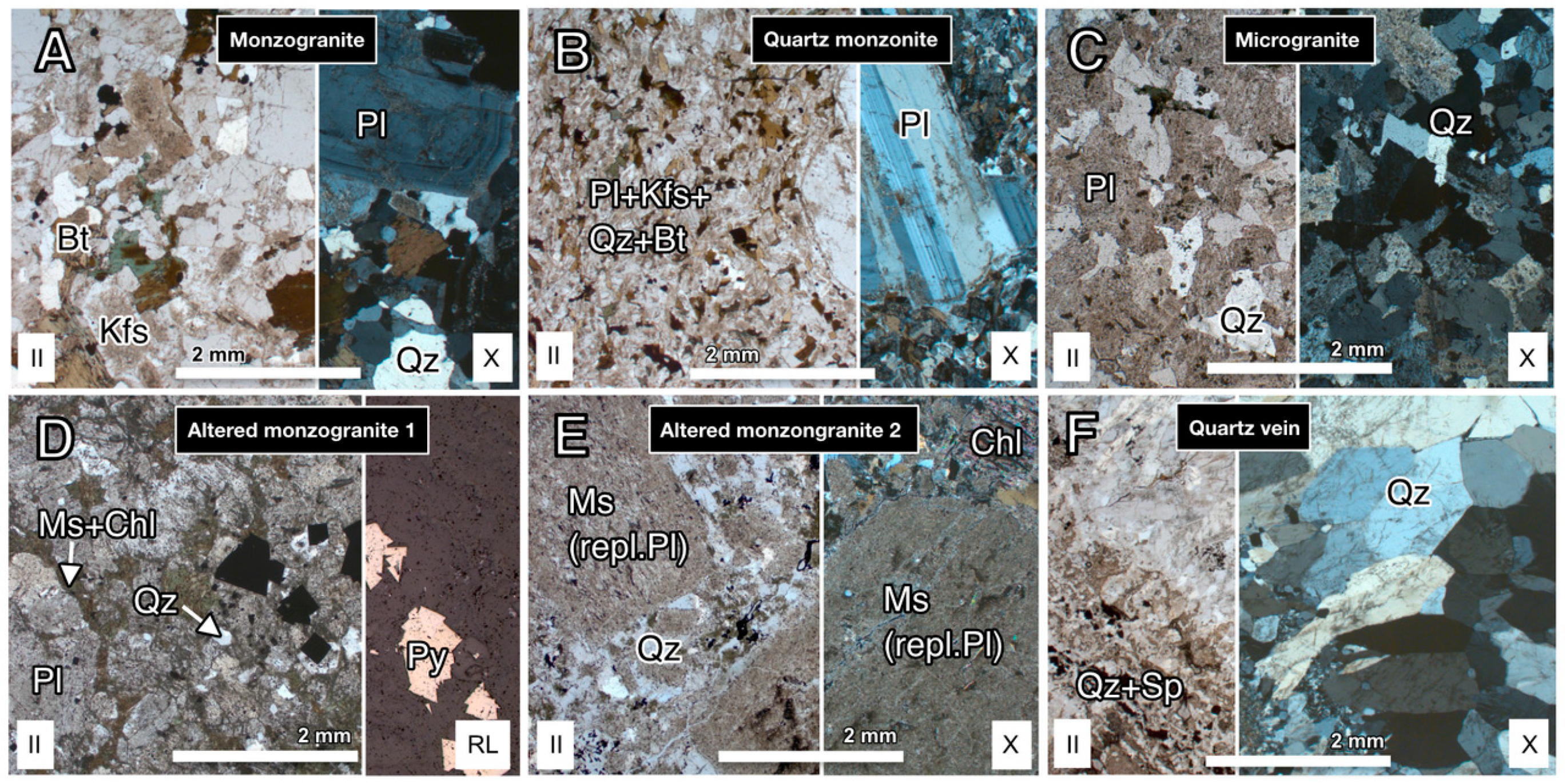
| Phase | wt.% ± 3σ | Phase | wt.% ± 3σ | Phase | wt.% ± 3σ | Phase | wt.% ± 3σ | Phase | wt.% ± 3σ | Phase | wt.% ± 3σ | |
| Pl (An10–50) | 38.2 ± 0.3 | Pl (An10–50) | 39.2 ± 0.4 | Pl (An0–16) | 34.1 ± 0.8 | Pl (An0–10) | 38.4 ± 1.0 | Qz | 60 1 | Qz | 91.2 ± 0.5 | |
| Qz | 29.3 ± 0.1 | Kfs | 22.2 ± 0.2 | Qz | 29.8 ± 0.6 | Qz | 31.6 ± 0.8 | Ms | 32 1 | Cal | 6.9 ± 0.5 | |
| Kfs | 20.3 ± 0.2 | Qz | 12.6 ± 0.1 | Kfs | 21.9 ± 0.8 | Ms | 12.7 ± 0.7 | Kln | 8 1 | Py | 1.6 ± 0.2 | |
| Chl | 8.0 ± 0.2 | Chl | 10.1 ± 0.3 | Chl | 6.6 ± 0.8 | Chl | 9.5 ± 0.9 | Sp (Fe) | 0.3 ± 0.2 | |||
| Bt | 4.2 ± 0.1 | Ilt | 5.3 ± 0.1 | Bt | 5.0 ± 0.4 | Py | 3.9 ± 0.3 | |||||
| Bt | 4.9 ± 0.1 | Cal | 2.6 ± 0.4 | Cal | 3.5 ± 0.5 | |||||||
| Fprg | 4.6 ± 0.1 | Sp (Fe) | 0.4 ± 0.1 | |||||||||
| Ap | 1.0 ± 0.0 | |||||||||||
| Dataset | RMSE X [m] | RMSE Y [m] | RMSE Z [m] |
|---|---|---|---|
| UAV VNIR | 0.04 | 0.06 | 0.06 |
| Terr. VNIR–SWIR | 0.15 | 0.21 | 0.28 |
| Terr. LWIR | 0.16 | 0.13 | 0.11 |
© 2018 by the authors. Licensee MDPI, Basel, Switzerland. This article is an open access article distributed under the terms and conditions of the Creative Commons Attribution (CC BY) license (http://creativecommons.org/licenses/by/4.0/).
Share and Cite
Kirsch, M.; Lorenz, S.; Zimmermann, R.; Tusa, L.; Möckel, R.; Hödl, P.; Booysen, R.; Khodadadzadeh, M.; Gloaguen, R. Integration of Terrestrial and Drone-Borne Hyperspectral and Photogrammetric Sensing Methods for Exploration Mapping and Mining Monitoring. Remote Sens. 2018, 10, 1366. https://doi.org/10.3390/rs10091366
Kirsch M, Lorenz S, Zimmermann R, Tusa L, Möckel R, Hödl P, Booysen R, Khodadadzadeh M, Gloaguen R. Integration of Terrestrial and Drone-Borne Hyperspectral and Photogrammetric Sensing Methods for Exploration Mapping and Mining Monitoring. Remote Sensing. 2018; 10(9):1366. https://doi.org/10.3390/rs10091366
Chicago/Turabian StyleKirsch, Moritz, Sandra Lorenz, Robert Zimmermann, Laura Tusa, Robert Möckel, Philip Hödl, René Booysen, Mahdi Khodadadzadeh, and Richard Gloaguen. 2018. "Integration of Terrestrial and Drone-Borne Hyperspectral and Photogrammetric Sensing Methods for Exploration Mapping and Mining Monitoring" Remote Sensing 10, no. 9: 1366. https://doi.org/10.3390/rs10091366